First-principles modeling of the Invar effect in Fe₆₅Ni₃₅ by the spin-wave method

Abstract

Thermal lattice expansion of the Invar Fe_0.65Ni_0.35 alloy is investigated in first-principles calculations using the spin-wave method, which is generalized here for the ferromagnetic state with short range order. It is shown that magnetic short-range order effects make substantial contribution to the equilibrium lattice constant and cannot be neglected in the accurate ab initio modeling of the thermal expansion in Fe-Ni alloys. We also demonstrate that at high temperatures, close and above the magnetic transition, magnetic entropy associated with transverse and longitudinal spin fluctuations yields a noticeable contribution to the equilibrium lattice constant. The obtained theoretical results for the temperature dependent lattice constant are in semiquantitative agreement with the experimental data apart from the region close the magnetic transition.

I Introduction

Magnetic and structural transformations in Fe are the origin of a large variety of Fe-based alloys with diverse mechanical and magnetic properties, which can be obtained by the proper alloying and processing these materials. The fcc Invar FeNi-based alloys are an example of such a tuning using an alloy composition, which results in the anomalously low thermal expansion known as the Invar effect.guillaume1897 It exists in a relatively narrow range of compositions: between  30 and  45 at.% of Ni and most distinct at 35 at. % of Ni.at-wt It can be made even more pronounced using other alloying schemes.superInvar

The fact that the Invar effect (as well as the Elinvar effect) is somehow related to magnetism was understood by Guillaume a century ago who started his Noble lectureguill_nl from a description of magnetic properties, namely the magnetic transition temperatures of Fe-Ni alloys, although at that time, there was no sensible theory of magnetism in solids. Only in 1963, Weiss made that connection clear in his well-known 2$\gamma$-state modelweiss63 arguing that the usual thermal lattice expansion due to the lattice anharmonicity was compensated in the Fe-Ni alloys by a temperature induced ”electronic” transition of the states with a higher moment and a large volume to the high temperature states having a lower magnetic moment and volume.

What was, however, confusing in the Weiss model is the identification of the high-temperature ”$\gamma$-phase” as antiferromagnetic. Thirty years later, the low volume and low magnetic moment state was discovered in a number of ferromagnetic first-principles calculations.moruzzi90 ; mohn91 ; entel93 ; schroter95 ; entel97 ; podgorny92 ; peperhoff01 The connection to the Invar effect due to thermal spin excitations then was accomplished using a phenomenological Ginzburg-Landau model.

Unfortunately, these calculations and models have little to do with the finite temperature magnetic state in the real Invar Fe-Ni alloys, which is ferromagnetic with a certain degree of randomness leading to the lowering of the magnetization with temperature. The origin of the problems with these earlier ab initio calculations is the use of the local spin density approximation, which is as well-known nowadays, significantly underestimate the equilibrium volume of 3d-metals and their alloys. So, the theoretical equilibrium volume was too small and close to the so-called low-spin – high-spin transition, which was not actually the case of the real Fe₆₅Ni₃₅ alloys.

The first adequate semi-empirical theory of the Invar effect was developed by Kakehashikakehashi81 ; kakehashi89 who explained it by a reduction of the local moments of Fe due to temperature induced magnetic disorder. Such a reduction of the magnetic moment in the magnetically disordered state compared to the ground state ferromagnetic one was for the first time confirmed in the first-principles calculations by Johnson et al. johnson90 ; johnson97 using the disordered local moment (DLM) modelgyorffy85 for the paramagnetic state and later by Akai and Dederichs.akai93

Thus the qualitative picture of the Invar effect is related to the reduction of the equilibrium 0 K ground state volume of the finite-temperature ferromagnetic phase due to the increasing randomness of the magnetic configuration. If one assumes that the thermal expansion due to the lattice anharmonicity is fixed, i.e. does not depend on temperature, the description of the Invar effect will be reduced to the finding the 0 K equilibrium volume of the alloy in the magnetic state with the reduced magnetization, which corresponds to the given temperature.

This simple model was used in the first-principles calculations by Crisan et al.crisan02 who almost quantitatively reproduced the experimental thermal expansion coefficient of Fe₆₅Ni₃₅ between 0 and 1000 K. Although some of the details of this modeling are questionable,ruban07 nevertheless, this was the first ab initio investigation, which reproduced the Invar effect.

Similar first-principles-based modeling of the Invar effect, using 0 K total energies of alloys with different spin configurations representing the finite-temperature magnetic state of the Invar alloy, was successfully applied by Khmelevskyi et al. to a number of different Invar systems,khmelevskyi03 ; khmelevskyi04a ; khmelevskyi04b ; khmelevskyi05 ; ruban07 A more elaborate approach was adopted by Liot and co-authors liot09 ; liot12 ; liot14 who actually calculated the finite temperature lattice constant and thermal expansion coefficient of some Invar alloys using the Debye-Grüneisen model.moruzzi88

It is obvious, that the above mentioned computational schemes are approximate in many details. The most important one, especially in the case of Fe-Ni Invar alloys, is a quite approximate description of the finite temperature magnetic state in the DFT based calculations. Unfortunately, going beyond DFT with the proper quantitative modeling of the Invar effect is unrealistic at the present time. Nevertheless, until the proper methods and computers are available, one can still try to improve the existing DFT-based models.

In particular, in this work, a more elaborate model of the thermal expansion in the Invar Fe₆₅Ni₃₅ alloy is developed. It 1) includes a consideration of the magnetic short-range order (MSRO) effects both below and above the Curie temperature and 2) takes into consideration magnetic entropy related to the temperature induced spin fluctuations. The MSRO effects are incorporated using the spin-wave method (SWM),ruban12 which is generalized here for the ferromagnetic state with arbitrary magnetization.

Heisenberg Monte Carlo simulations with magnetic exchange interaction parameters obtained in first-principles calculations, are done to determine the magnetic state characterized by the corresponding magnetic short- and long-range order (LRO) for every temperature. This information is used in the SWM calculations to get the total energy of the system in the given magnetic state and parameters of the Debye-Grüneisen model yielding finally the lattice constantmoruzzi88 ; korzhavyi94 at the corresponding temperature.

II Spin-wave method for systems with magnetic long- and short-range order

The SWM is based on the assumption that the magnetic energy of a system is given by Heisenberg Hamiltonian

$$H=-\sum_{p}\sum_{i,j\in p}J_{p}\mathbf{e}_{i}\mathbf{e}_{j},$$ (1)

where $J_{p}$ are the magnetic exchange interaction parameters, which do not depend on the magnetic state; $p$ is the coordination shell and $\mathbf{e}_{i}$ is the direction of the magnetic moment at site $i$.

For such a Hamiltonian, the magnetic configuration is uniquely identified by spin-spin correlation functions

$$\xi_{p}\equiv<\mathbf{e}_{i}\mathbf{e}_{j}>_{p}=\frac{1}{Nz_{p}}\sum_{i,j\in p}\mathbf{e}_{i}\mathbf{e}_{j},$$ (2)

where $N$ is the number of atoms and $z_{p}$ is the coordination number. The magnetic energy of a system presented by Hamiltonian (1) then can be determined as

$$E=-\sum_{p}J_{p}z_{p}\xi_{p}=-\sum_{\mathbf{R}}J(\mathbf{R})\xi(\mathbf{R}).$$ (3)

Since, in the ideal paramagnetic (IPM) state $\xi(\mathbf{R})=0$, and therefore (3) is just the energy of the magnetic long- and short-range order.

Using the following definition of the Fourier transform of the spin-spin correlation function

$$\xi(\mathbf{q})=\sum_{\mathbf{R}}\xi(\mathbf{R})e^{i\mathbf{qR}},$$ (4)

magnetic energy (3) can be determined in another form:

$$E=\frac{1}{\Omega_{BZ}}\int_{BZ}d\mathbf{q}J(\mathbf{q})\xi(\mathbf{q}),$$ (5)

where $J(\mathbf{q})$ is the Fourier transform of the magnetic exchange interactions (see, for instance, Ref. halilov98, ):

$$J(\mathbf{q})=-\sum_{\mathbf{R}}J(\mathbf{R})e^{i\mathbf{qR}},$$ (6)

which is, up to an additive constant, just the energy of the planar spin-spiral (PSS) with wave vector $\mathbf{q}$.

The spin-spin correlation function of such a PSS issandratskii98

$$\xi_{\mathbf{q}}(\mathbf{R})=\cos(\mathbf{qR}),$$ (7)

and the equally weighted superposition of all the PSS with different wave vectors $\mathbf{q}$ yields the IPM since

$$\frac{1}{\Omega_{BZ}}\int_{BZ}d\mathbf{q}\xi_{\mathbf{q}}(\mathbf{R})=\xi(\mathbf{R})=0$$ (8)

for all $\mathbf{R}$ except for $\mathbf{R}=0$, which $\xi(\mathbf{R}=0)=1$.

The Fourier transform of $\xi_{\mathbf{q}}(\mathbf{R})$ for some specific $\mathbf{q}^{\prime}$ is the Dirac $\delta$-function, $\xi_{q}(\mathbf{q^{\prime}})=\delta(\mathbf{q}-\mathbf{q}^{\prime})$, and therefore the following important normalization condition holds:

$$\frac{1}{\Omega_{BZ}^{2}}\int_{BZ}d\mathbf{q}\int_{BZ}d\mathbf{q}^{\prime}\xi_{\mathbf{q}}(\mathbf{q}^{\prime})=1.$$ (9)

This means that the PSS form a complete and orthogonal basis with eigenvalues $E(\mathbf{q})$, which are in general the total energies of a system within some general Hamiltonian, in the the PSS magnetic configuration with wave vector $\mathbf{q}$. In the case of Heisenberg Hamiltonain (1), $E(\mathbf{q})=J(\mathbf{q})$. If $E(\mathbf{q})$ is obtained in first-principles calculations and the magnetic energy of the system can be described by Hamiltonian (1), $E(\mathbf{q})=J(\mathbf{q})+E_{0}$, where, as will be shown below, $E_{0}$ is the total energy of the IPM obtained in the same first-principles calculations.

The energy of the IPM state within the first-principles formalism, can be found using the fact that its real space spin-spin correlation functions are given by the equal weighted superposition of all the PSS in the reciprocal space (8). Then one can use (5) by substituting $E(\mathbf{q})$ instead of $J(\mathbf{q})$, which defines the energy of specific magnetic configuration given by a set of spin-spin correlation functions, $\xi(\mathbf{R})$ or equivalently $\xi(\mathbf{q})$, so that

$$E^{\rm IPM} = \frac{1}{\Omega_{BZ}^{2}}\int_{BZ}d\mathbf{q}E(\mathbf{q})\int_{BZ}d\mathbf{q}^{\prime}\xi_{\mathbf{q}}(\mathbf{q}^{\prime})$$

$$= \frac{1}{\Omega_{BZ}}\int_{BZ}d\mathbf{q}\ E(\mathbf{q}).$$

If one uses $J(\mathbf{q})$ instead of $E(\mathbf{q})$ in (II), the last integral is formally equal to $J(\mathbf{R}=0)$, which is routinely accepted to be zero in (1). Thus $E^{\rm IPM}=E_{0}$ and it indeed connects the Fourier transform of the magnetic exchange interactions of Hamiltonian (1) $J(\mathbf{q})$ and $E(\mathbf{q})$ from first-principles calculations.

The presence of the MSRO leads to a deviation of $\xi^{\rm SRO}(\mathbf{q})$, or simply $\xi(\mathbf{q})$, from the equal weighted distribution of the PSS in the reciprocal space. However, its does not violate the normalization of the expansion in terms of the PSS since

$$\frac{1}{\Omega_{BZ}}\int_{BZ}d\mathbf{q}\xi(\mathbf{q})=0,$$ (11)

and thus the energy of the MSRO is

$$\Delta E^{\rm SRO}=\frac{1}{\Omega_{BZ}}\int_{BZ}d\mathbf{q}\ E(\mathbf{q})\xi(\mathbf{q}).$$ (12)

Then the total energy is given by the sum of the energy of the IPM state and MSRO:

$$E=\frac{1}{\Omega_{BZ}}\int_{BZ}d\mathbf{q}\ E(\mathbf{q})\left(1+\xi(\mathbf{q})\right),$$ (13)

The later expression defines the energy of paramagnetic state with MSRO and can be used in first-principles calculations.

The outlined above formalism should be modified in the presence of magnetic long-range order. Here, it is done for the ferromagnetic state. In this case, spin-spin correlation functions $\xi(\mathbf{R})$, and respectively $\xi(\mathbf{q})$, can be divided below the Curie temperature into two contributions: from the long-range order, $s_{0}$, and short-range order, $\xi^{\rm SRO}(\mathbf{R})$, defined in the following way:

$$s_{0}=\lim_{R\to\infty}\xi(\mathbf{R});$$ (14)

$$\xi^{\rm SRO}(\mathbf{R})=\xi(\mathbf{R})-s_{0}.$$ (15)

It is clear that $s_{0}$ is the long-range order parameter, or the reduced magnetization in the case of a ferromagnet.

The Fourier transform of $\xi(\mathbf{R})$ will contain then also two contributions: from the long-range order, which is $s_{0}\delta(\mathbf{q}-0)$ and the contribution from the short-range order part, $\xi^{\rm SRO}(\mathbf{q})$, which is the Fourier transform of $\xi^{\rm SRO}(\mathbf{R})$. The later does not contribute to the total normalization, and therefore, in order to have the proper normalization, one should add the completely random background compensating the missing part from the long-range order contribution, i.e. normalized by $1-s_{0}$. Thus, the total energy of the FM state with reduced magnetization $s_{0}$ is

$$E = s_{0}E(\mathbf{q}=0)+$$

$$\frac{1}{\Omega_{BZ}}\int_{BZ}d\mathbf{q}\ E(\mathbf{q})\left[1-s_{0}+\xi^{\rm SRO}(\mathbf{q})\right].$$

The first term is just the energy of the completely ordered FM state, while the second one is the contribution from the randomly oriented magnetic moments (with some MSRO), which reduces the magnetization of system from its completely ordered value.

If one neglects the SRO effects in the second term, i.e. if $\xi^{\rm SRO}(\mathbf{q})=0$, Eq. (II) defines the so-called partial disordered local moment (PDLM) model, which is used for the modeling of a ferromagnetic state at finite temperatures within the coherent potential approximation (CPA) calculations.

III Details of ab initio calculations

According to the existing experimental datarobertson99 ; tsunoda08 as well as the results of first-principles modeling,ruban07 Fe-Ni Invar alloys are random, without noticeable atomic short-range order. The easiest way to determine the electronic structure and the total energy of such alloys is to use the CPA,CPA which works very well for this systems as has been demonstrated previouslyruban07 and also confirmed in this work. The CPA calculations have been done in the framework of the Green’s function EMTO method.andersen94 ; andersen98 ; vitos01 In particular, the Lyngby version of the EMTO code has been used, which allows non-collinear and spin-spiral calculations as well as the correct treatment of the screened Coulomb interactions within the single site approximation.ruban02 In the latter case, the on-site screened electrostatic potential, $V^{i}_{scr}$, and energy, $E^{i}_{scr}$ruban02 , are

$$v_{scr}^{i} = -e^{2}\alpha_{scr}\frac{q_{i}}{S}$$ (17)

$$E^{i}_{scr} = -e^{2}\frac{1}{2}\alpha_{scr}\beta_{scr}\frac{q_{i}^{2}}{S}.$$ (18)

Here $q_{i}$ is the net charge of the atomic sphere of the $i$th alloy component, $S$ the Wigner-Seitz (WS) radius, and $\alpha_{scr}$ and $\beta_{scr}$ the on-site screening constants. The screening constants of a random Fe₆₅Ni₃₅ alloy in the FM and DLM states have been obtained in the 560-atom supercell locally-self consistent Green’s function (LSGF)abrikos97 calculations using the ELSGF methodpeil12 including the first two coordination shells in the local interaction zone.abrikos97 The screening constants are found to be very little dependent on the magnetic state and the lattice constant, and $\alpha_{scr}=$ 0.8 and $\beta_{scr}=$1.14, have been then used in all the EMTO-CPA calculations.

The basis functions in all the EMTO calculations have been expanded up to $l_{max}=$3. We have also taken into consideration the multipole moment contributions to the electrostatic energy. The summation over multipole moments for the electrostatic part of the one-electron potential and total energy have been carried out up to $l_{max}=$6. The integration over the irreducible part of the Brillouin zone has been performed using the 36$\times$36$\times$36 Monkhorst-Pack grid.monkhorst72

The self-consistent calculations have been done within the local density approximation (LDA),LDA92 while the total energy has been obtained using the PBE generalized gradient functional (GGA).pbe96 The point is that the LDA self-consistency does not affect the final GGA total energy, but it affects the magnitude of the magnetic moment, which is usually slightly overestimated in the PBE-GGA compared with the LDA one.

In spite of the existing theoretical investigation of local lattice relaxations in Fe₆₅Ni₃₅ in the FM state,liot09rel nothing is known about their effect on the thermal lattice expansion and the Invar effect, in particular. Therefore, in order to estimate the role of local lattice relaxations in the energetics of Fe-Ni Invar alloys, we have calculated the equilibrium lattice constants and total energies of a 64-atom supercell (4$\times$4$\times$4) modeling Fe_62.5Ni_37.5 random alloyscell with relaxed (locally) and unrelaxed atomic positions.

The PBE-GGA calculations have been done by the projector augmented wave (PAW) methodblochl94 ; kresse99 as implemented in the Vienna ab initio simulation package (VASP) code.kresse93 ; kresse94 ; kresse96 We find that the lattice constant of the supercell with relaxed atomic positions is only 0.0006 Å smaller than that of the unrelaxed one. The relaxation energy is also small: 7 meV/atom. This means that local lattice relaxations can hardly have any effect on the Invar effect, which is in fact expected from the relatively small size difference of Fe and Ni.

IV Models of finite temperature magnetism in Fe-Ni alloys

Magnetism plays crucial role in the Invar effect, which exists in Fe-Ni alloys in the FM state. However, the paramagnetic state is not less important, since it determines the type of thermal magnetic excitations both above and below the Curie temperature. In all the previous ab initio modeling of the Invar effect in FeNi, it has been tacitly assumed that the main thermal magnetic excitations is the thermal disorder of the orientation of the local magnetic moments, which magnitude remains unchanged, or transverse spin fluctuations (TSF).

However, the magnitude of the local magnetic moments on Fe and Ni in Fe₆₅Ni₃₅ is quite sensitive to the magnetic state, and, for instance, the magnetic moment on Ni vanishes in the DLM representation of the paramagnetic state. This does not correspond to what really happens in the paramagnetic state at finite temperature, where non-zero magnetic moment exists due to an entropic effect of thermally induced longitudinal spin fluctuations (LSF). As will be demonstrated below, the LSF play important role in Fe₆₅Ni₃₅ and therefore, in this section, we introduce a simplified model of the LSF, which will be used further both in the calculations of magnetic exchange interactions and in the modeling of the thermal lattice expansion.

IV.1 Longitudinal spin fluctuations in Fe₆₅Ni₃₅

Unfortunately, accurate first-principles modeling of the LSF is too cumbersome for the case of random alloys. An approximate DFT-based model developed in Ref. ruban07_lsf, is also quite complicated for Fe-Ni alloys due to pronounced local chemical environment effects,ruban05 which require an additional consideration of different possible local atomic configurations. Therefore, a simple model is used here for just for a qualitative estimate of LSF, which has been previously introduced in Ref. ruban13, .

Here, we consider LSF in the paramagnetic state given by the DLM model assuming that they are adiabatically connected with a particular electronic structure, which results in specific magnitudes of the local magnetic moments of alloy components. In this case, the local magnetic moment of specific alloy component, $i$, at a given temperature T can be determined in the single-site mean-field approximation asruban13 ; sandratskii08

$$<m_{i}>=\frac{\int m^{3}\exp\left[-\beta E^{\rm LSF}_{i}(m)\right]dm}{\int m^{2}\exp\left[-\beta E^{\rm LSF}_{i}(m)\right]dm},$$ (19)

where, $\beta=1/T$ and $E^{\rm LSF}_{i}(m)$ is the so-called LSF energy of the $i$th component, which is the total energy of an alloy per atom of this alloy component. It is determined here for each alloy component in the constrained DLM-CPA calculations by fixing the local magnetic moment of alloy component $i$, while allowing the magnetic moment of the other alloy component to relax to the corresponding self-consistent magnitude.

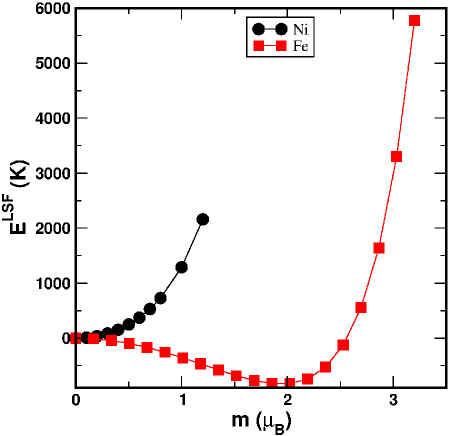
Figure 1: (Color online) LSF energy of Ni and Fe in random Fe₆₅Ni₃₅ at 1000 K.

In Fig. 1, the LSF energy of Ni and Fe in Fe₆₅Ni₃₅ is shown for the lattice constant of 3.59 Å. The calculations are done at 1000 K and the LSF energy contains also the entropy contribution from the one-electron excitations and in the case of the LSF energy of Ni also contribution from the magnetic entropy of Fe taking in the usual form of the magnetic entropy of paramagnetic gas:

$$S^{\rm TSF}=\ln(m^{\rm Fe}+1),$$ (20)

where $m^{\rm Fe}$ is the magnetic moment of Fe in the DLM-CPA calculations. The latter, in fact, corresponds to the magnetic entropy of the TSF. Thus, the LSF energy of Ni contains also the entropy contribution from the one-electron excitations on both components and magnetic entropy (20) on Fe.

This approach, however, does not work for the LSF energy of Fe, since the magnetic moment of Ni vanishes in the DLM-CPA calculations and therefore one should consider LSF on Ni at the given temperature. As has been demonstrated in Ref. ruban13, , if the LSF energy has a quadratic form (as a function of magnetic moment), the LSF entropy is

$$S^{\rm LSF}=3\ln(<m_{i}>),$$ (21)

where $<m_{i}>$ is the average magnitude of magnetic moment of the $i$th alloy component. This expression is valid in the high-temperature (classical) limit. In the single site approximation, one can simply substitute $<m_{i}>$ by $m_{i}$, and $m_{i}$ can be found from the free energy minimization of the alloy.

The latter is however a quite tedious procedure. Fortunately, this task can be substantially simplified in the DFT self-consistent calculations if one notice that such a minimization results in the appearance of an additional contributions to the one-electron potential, which can be obtained from the corresponding functional derivatives of (21) with respect to spin-up and spin-down densities.korzhavyi Then the magnetic moment induced by the LSF at a given temperature is just the result of the corresponding DFT self-consistent calculations, which simplifies enormously the whole calculation procedure.

Therefore, in order to account for the (qualitatively) correct magnetic state of Ni during the LSF energy calculations of Fe, the LSF on Ni were taken into consideration using (21) at 1000 K and adding the corresponding entropy term to the total energy of the alloy.

Although the LSF energy of Ni does not have the exact quadratic form, Eq. (21) still provides reasonable description of the LSF entropy. For instance, it yields 0.70 $\mu_{B}$ for the local magnetic moment of Ni in Fe₆₅Ni₃₅ at 1000 K, while a more accurate result from (19) is 0.82 $\mu_{B}$. At the same time, it is clear that (21) somewhat underestimates the magnetic entropy related to the LSF on Ni atoms in Fe₆₅Ni₃₅ and consequently the magnetic moment of Ni in the paramagnetic state at high temperatures.

The LSF energy of Fe is quite different from that of Ni: its minimum is at 1.77 $\mu_{B}$, although it is quite shallow with a steep increase beyond 2.5 $\mu_{B}$. Although the LSF energy of Fe does not resemble parabola, the magnetic moment of Fe due to the LSF is about 1.8 $\mu_{B}$ at 1000 K, independently if (21) or (19) are used in the calculations. One can also see, that the LSF affect little the magnitude of magnetic moment. However, as will be shown below, the magnetic entropy of Fe affects substantially the thermal lattice expansion in the paramagnetic state.

IV.2 Magnetic exchange interactions in Fe₆₅Ni₃₅

Magnetic state given by the corresponding spin-spin correlation functions, and its temperature dependence are key parameters needed for a quantitatively accurate modeling of the Invar effect. Although there exist experimental data on the reduced magnetization,crange63 nothing is known about MSRO or spin-spin correlation functions in Fe-Ni alloys. Therefore the only way to get this information is to use theoretical simulations.

We assume that the magnetic energy and spin configuration of the Fe-Ni Invar alloys at particular temperature can be determined in statistical thermodynamics simulations using the following classical Heisenberg Hamiltonian:

$$H=-\sum_{p}\sum_{i,j\in p}\sum_{\alpha,\beta=\rm Fe,Ni}J_{p}^{\alpha\beta}c_{i}^{\alpha}c_{j}^{\beta}\mathbf{e}_{i}\mathbf{e}_{j}.$$ (22)

Here, $J_{p}^{\alpha\beta}$ are the magnetic exchange interactions between $\alpha$ and $\beta$ alloy components for coordination shell $p$ and $\mathbf{e}_{i}$ is the direction of the spin at site $i$; $c_{i}^{\alpha}$ takes on value 1 if site $i$ is occupied by atom $\alpha$ and 0 otherwise.

Of course, the Fe-Ni Invar alloys are not a Heisenberg system: the corresponding magnetic exchange interactions depend not only on the local and global magnetic state but also on the local chemical environment.ruban05 However, the dependence on the local environment is strongest in the completely ordered FM state and can be neglected in qualitative statistical thermodynamics simulations at elevated temperatures. Therefore we calculate magnetic exchange interactions in random alloys within the CPA using magnetic force theoremliecht87 as is implemented in the Lyngby version of the EMTO coderuban16 within the LDA.j_xc_LDA

As has been already mentioned, the magnetic exchange interactions in Fe-Ni alloys depend quite strongly on the magnetic state, as is also the case of magnetic exchange interactions in bcc Fe.ruban04 In Fig. 2, we show the magnetic exchange interactions in Fe₆₅Ni₃₅ random alloy as a function of magnetization, which have been determined in the CPA-PDLM model calculations in the same way as in Ref. ruban08, . In this case, the first-principles CPA calculations have been done for the following model alloy configuration: (Fe$\uparrow_{y}$Fe$\downarrow_{1-y}$)_cNi_1-c, where $y$ is connected to the reduced magnetization, $m$, as $m=1-2y$, and $c$ is the concentration of Fe.ruban08 That is, only Fe atoms are used for the modeling of the reduced magnetization, while Ni atoms are left to acquire the magnetic moment according to the self-consistent calculations.

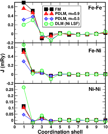
Figure 2: (Color online) Magnetic exchange interactions in random Fe₆₅Ni₃₅ alloy in the FM state with different magnetizations and in the paramagnetic state with LSF on Ni at 500 K, which is the Curie temperature of Fe₆₅Ni₃₅.

One can see that Fe-Ni and Ni-Ni magnetic exchange interactions decreasing together with decreasing magnetization, and in the paramagnetic state, when $m=0$, they should vanish in this model, since Ni magnetic moment disappears in the DLM-CPA calculations. This is not, however, the case if one consider the LSF on Ni at finite temperature. In Fig. 2, we show the Fe-Ni and Ni-Ni magnetic exchange interactions at 500 K (which is the Curie temperature of Fe₆₅Ni₃₅) due to the LSF on Ni. The latter were taking into consideration using (21) for the LSF entropy on Ni during DFT self-consistent calculations. As a result, the Fe-Ni and especially Ni-Ni magnetic exchange interactions at the first coordination shell become substantially larger than those in the FM state. This produces a pronounced effect on the Cuire temperature as will be demonstrated below.

IV.3 Magnetic transition in Fe-Ni alloys

The dependence of magnetic exchange interactions on the global magnetic state can be neglected in the calculations of the magnetic phase transition, which being the second order happens practically in the paramagnetic state (although with a large amount of the MSRO). In this case, one can chose only one set of magnetic interactions, which corresponds to the paramagnetic state just above the Curie temperature, and do statistical thermodynamics simulations of the magnetic transition. This is the corresponding state approach,ruban04 which has been, for instance, used before in the Curie temperature calculations of bcc Fe.

Here, we determine magnetic exchange interactions for the lattice constant and thermal one-electron excitations, which correspond to the experimental Curie temperature.crange63 ; hayase73 The use of the experimental Curie temperature in the calculations of the magnetic exchange interactions also simplifies the account for the LSF. As has been demonstrated above, the LSF on Ni lead to a substantial renormalization of the magnetic exchange interactions.

We have used two different schemes to account for the LSF on Ni: 1) DFT self-consistent calculations using (21) for the LSF entropy on Ni at a given temperature and 2) the use of the single-site mean-field approximation (19) for the average magnetic moment of Ni at a given temperature from the corresponding LSF energy. Although the second approach is quite time consuming, it is more accurate and this is important since magnetic exchange interactions are roughly proportional to the magnitude of the local magnetic moment.

In order to demonstrate that the described above method works reasonably well, we calculate the magnetic phase transition in several Fe-Ni alloys covering the whole concentration range of the fcc Fe-Ni alloys, including pure Ni. All the calculations have been done for random alloys using the CPA. The latter is probably a rough approximation for Ni-rich Fe-Ni alloys, where the Curie temperature is quite close to the atomic order-disorder phase transition. For instance, the Curie temperature of Fe₂₅Ni₇₅ is just about 100 K above the order-disorder phase transition. Nevertheless, we disregard the atomic short-range ordering going mainly after a qualitative picture.

Table 1: Calculated local magnetic moments on Ni in paramagnetic state due to LSF at the experimental Curie temperature and lattice constantscrange63 ; hayase73 from (21) and from (19) and theoretical and experimental Curie temperatures of some Fe-Ni alloys including pure Ni. The results obtained in the FM state are also shown for comparison.

Alloy	Fe65Ni35	Fe50Ni50	Fe30Ni70	Ni
mNi FM	0.75	0.71	0.66	0.62
mNi DLM-LSF;(21) for Ni	0.52	0.65	0.70	0.68
mNi DLM-LSF;(19) for Ni	0.66	0.69	0.66	0.58
Tc: Jxc FM	520	560	540	310
Tc: Jxc DLM-LSF;(21) for Ni	360	630	810	810
Tc: Jxc DLM-LSF;(19) for Ni	430	650	800	710
Tc Experiment	500	780	880	630

The calculated and experimental Curie temperatures are presented in Table 1. The theoretical Curie temperatures have been obtained in the Heisenberg Monte Carlo simulations using a simulation box of 12$\times$12$\times$12($\times$4) on the fcc underlying lattice. The transition temperature was determined approximately from the maximum of the heat capacity. Since the temperature step was 10 K, this is a kind of an error bar for the theoretical Curie temperatures.

One can see, that the Curie temperature is indeed sensitive to the magnitude of the Ni local magnetic moment. The overall best agreement of the calculated Curie temperature with experimental data is obtained using the magnetic moment from single-site mean-field modeling (19). As one can see in Table 1, the LSF entropy given by Eq. (21) underestimates the induced magnetic moment of Ni in the Fe-rich alloys and overestimates it in the Ni-rich alloys and pure Ni.

It is interesting, that the magnetic exchange interactions in the completely ordered FM state yield the best results for the Curie temperature of the Invar Fe₆₅Ni₃₅ alloy (see Table 1). However, the FM interactions do not reproduce the general trend of the concentration dependence of the Curie temperature in Fe-Ni alloys with maximum around 70 at.% of Ni. This is so since these alloys are not Heisenberg systems, and thus the FM exchange interactions are hardly relevant to the magnetic exchange interactions at the Curie temperature close to the paramagnetic state.

V Spin-wave method results for the 0 K total energy

V.1 Completely ordered ferromagnetic and ideal paramagnetic states

To get a reasonably accurate account for the MSRO, the integration over q-points in the SWM (see Eq. (II)) was done using the 7$\times$7$\times$7 Monkhorst-Pack grid,monkhorst72 which results in 20 non-equivalent q-points in the irreducible part of the fcc Brillouin zone. For every Wigner-Seitz (WS) radius within the range of 2.6 – 2.7 a.u. (with the step of 0.005 a.u.), the total energies of Fe₆₅Ni₃₅ alloy were calculated in the corresponding 20 PSS states by the EMTO-CPA method (see Appendix A and B for details). Then, for every WS radius, the total energy of Fe₆₅Ni₃₅ in the given magnetic state was obtained by the corresponding weighting of the total energies obtained in the PSS calculations (see Appendix B).

The total energy of the completely ordered ferromagnetic state is, of course, just the total energy of the PSS with $\mathbf{q}=0$. The total energy of the IPM state is given by the equal weighted sum of the total energies of all spin-spirals. Another way to calculate the total energy of the IPM state is to do collinear DLM-CPA calculations. For a Heisenberg system these two methods should produce the same energy.

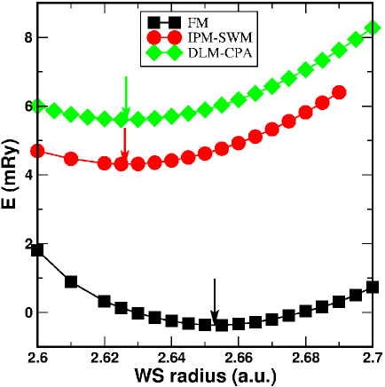
Figure 3: (Color online) Total energy of random Fe₆₅Ni₃₅ in the FM and PM states. The latter is obtained in the CPA-DLM (diamonds) and SWM (circles) calculations. The arrows show the position of equilibrium WS radii.

However, it is not the case of Fe₆₅Ni₃₅. As is seen in Fig. 3, the energy of the IPM state in the SWM is 1 mRy lower than the DLM-CPA energy. At the same time, the FM energy is only about 5 mRy below the energy of the paramagnetic state. The reason of such disagreement between the DLM-CPA and SWM total energies is a pronounced itinerant electron character of magnetism in this alloy. It is also reflected in the difference of the local magnetic moments of Fe and Ni in the IPM state. While the local magnetic moment of Ni vanishes in the DLM-CPA calculations, its average magnitude in the SWM is about 0.1 $\mu_{B}$.

The latter is due to the contributions from long wave PSS. The magnetic moment of Fe in the SWM calculations is also larger than that obtained in the DLM-CPA calculations for the same reason. At the same time, the magnetic moment of Fe in the paramagnetic state is substantially smaller than one in FM state, as one can see in Fig. 4.

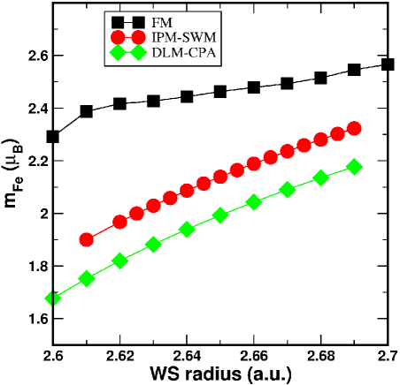
Figure 4: (Color online) Local magnetic moment of Fe in Fe₆₅Ni₃₅ as a function of the WS radius in the FM and paramagnetic states.

Let us note that in spite of all the above mentioned differences in results for energies and magnetic moments, the SWM and DLM-CPA agree on the equilibrium volume or WS radius, of the IPM state. The later is about 2.626 a.u. in both cases (which corresponds to the lattice constant of 3.554 Å). The equilibrium WS radius in the FM state, $S^{\rm FM}$ is 2.653 a.u. (lattice constant is 3.593 Å, without contribution from zero point lattice vibrations). This is exactly what was reported in the previous EMTO calculations.ruban07

V.2 Magnetic short-range order effects

In the SWM, the MSRO effects are taken into consideration through the corresponding spin-spin correlation functions. In this work, the spin-spin correlation functions have been obtained in the Heisenberg Monte Carlo simulations described in Sec. IV.3. Although those calculations have been done for a fixed set magnetic exchange interactions which correspond to the paramagnetic state, the calculated reduced magnetization of Fe₆₅Ni₃₅ turns out to be in good agreement with the experimental one crange63 in the whole temperature range, as is shown in Fig. 5. Therefore we expect that the theoretical results for the spin-spin correlation functions are qualitatively correct and can be used in the SWM modeling.

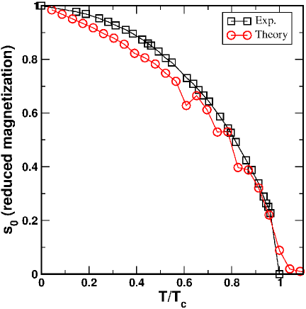
Figure 5: (Color online) Reduced magnetization as a function of reduced temperature in Fe₆₅Ni₃₅ : Experimentcrange63 vs present theoretical modeling.

Since the homogenous magnetic state is assumed in the single-site CPA spin-spiral calculations of Fe₆₅Ni₃₅, the component-resolved spin-spin correlation functions from the Monte Carlo simulations should be reduced to the average ones consistent with the first-principles spin-spiral calculations in order to be used in the SWM. For the completely random alloy, the average spin-spin correlation function is

$$\tilde{\xi}(\mathbf{R}) = c^{2}\xi^{\rm Fe-Fe}(\mathbf{R})+2c(1-c)\xi^{\rm Fe-Ni}(\mathbf{R})$$

$$+ (1-c)^{2}\xi^{\rm Ni-Ni}(\mathbf{R}),$$

where $\xi^{\rm Fe-Fe}(\mathbf{R})$, $\xi^{\rm Fe-Ni}(\mathbf{R})$, and $\xi^{\rm Ni-Ni}(\mathbf{R})$ are the Monte Carlo results for the spin-spin correlation functions of different alloy pairs.

In fact, the difference between these three alloy-component resolved spin-spin correlation functions is quite small in the FM state, and becomes pronounced only at high temperatures, especially for distant coordination shells. However, in the latter case, the correlation functions themselves become quite small. For instance, the largest nearest neighbor spin-spin correlation functions at 300 K are 0.820, 0.750, and 0.677, while at 1000 K they are 0.091, 0.070, and 0.024 for Fe-Fe, Fe-Ni, and Ni-Ni pairs, respectively. This means that averaging (V.2) does not introduce a noticeable error.

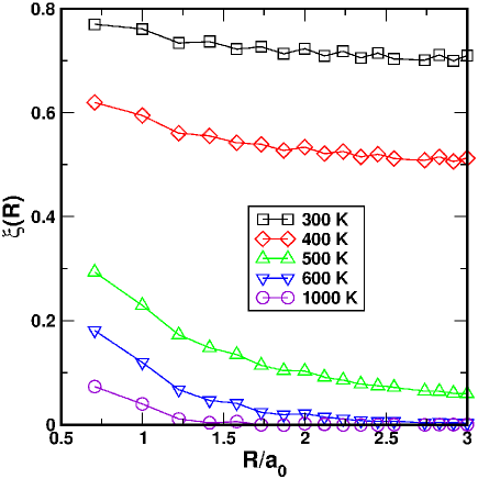
Figure 6: (Color online) Average spin-spin correlation function in Fe₆₅Ni₃₅ at different temperatures.

The spatial behavior of the spin-spin correlation functions is shown in Fig. 6. In the totally ordered FM state, $\tilde{\xi}(\mathbf{R})=1$, and in the IPM ,$\tilde{\xi}(\mathbf{R})=0$. In the PDLM model for the FM state with reduced magnetization $s_{0}$, $\tilde{\xi}(\mathbf{R})=s_{0}$. One can see, that the MSRO becomes important close to the magnetic phase transition, exactly where the Invar effect is observed.

The average spin-spin correlation functions have been used in the SWM calculations in order to get the total energy of Fe₆₅Ni₃₅ at a given temperature (see Appendix B for details). Since the calculated Curie temperature and theoretical one differs, the theoretical temperature dependence of the spin-spin correlation functions has been rescaled in order to have the Curie temperature and MSRO consistent with the experiment.crange63

In Fig. 7, we show the results for the 0 K equilibrium lattice constant of Fe₆₅Ni₃₅ obtained in the SWM calculations from the spin-spin correlation functions at the corresponding temperature, which is shown on the x-axis. On the same figure, we also show the results of the PDLM-CPA calculations, where the mapping to the temperature is done only according to the reduced magnetization since the MSRO effects are absent in the PDLM-CPA model. The latter is, in particular, the reason for the abrupt change of the lattice constant at 500 K, which is the Curie temperature, and its constant value above the magnetic phase transition. It is clear that the MSRO effects are pronounced and cannot be neglected in the accurate ab initio modeling of the Invar effect.

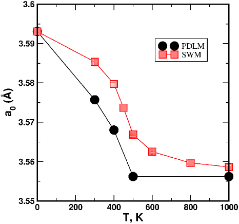
Figure 7: (Color online) Zero temperature lattice constant obtained in the SWM and PDLM calculations as a function of magnetic state translated to the corresponding temperature shown on the x-axis.

VI Calculated thermal lattice expansion

VI.1 Debye-Grüneisen model

As has been mentioned above, the Debye-Grüneisen modelmoruzzi88 ; korzhavyi94 is the only way to account for the thermal lattice expansion in the FeNi Invar alloys at present time. A combination of chemical randomness with highly non-trivial thermal electronic and magnetic excitations leave no chance, for instance, for using quasiharmonic approximation based on the ab initio phonon calculations.

Three parameters are needed for the Debye-Grüneisen modeling: bulk modulus, Grüneisen constant, and zero-temperature equilibrium lattice constant. However, it is quite difficult to obtain stable results for the Grüneisen constant, especially in the FM state, where the magnetic moment of Fe does not change linearly (see Fig. 4).

In the present study, the Morse fitmoruzzi88 was used for a parametrization of the total energy (or the Helmholtz free energy) as well as for determining the parameters of the Debye-Grüneisen model, which seemed to be quite stable and not so sensitive to the range of energy fitting, the size of the step, and other details. But even in this case, the calculated Grüneisen constant exhibited some fluctuations related to the details of calculations. So, in the end, in order to simplify the tedious numerical exercise, its value was fixed to 1.8, which is close to the obtained values also by Liot et al.liot09 , for all the Debye-Grüneisen calculations, which were done using the formalism outlined in Ref. korzhavyi94, .

VI.2 Transverse and longitudinal spin fluctuations in the ideal paramagnetic state

Before we discuss the effect of the MSRO, we would like to demonstrate the effect of spin fluctuations on the temperature dependence of the lattice constant of Fe₆₅Ni₃₅ in the IPM. The starting point here is the total energy of the IPM state without contributions from the electronic and magnetic thermal excitations. In Fig. 8, the corresponding lattice constants obtained in the Debye-Grüneisen model from the DLM-CPA and SWM total energies (E) are shown. They agree well with each other and with the results by Liot and Hooleyliot12 obtained in the similar DLM-CPA calculations.

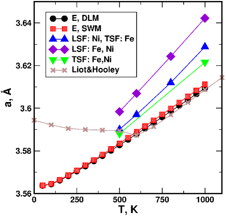
Figure 8: (Color online) Temperature dependence of the lattice constant of the IPM of Fe₆₅Ni₃₅ obtained in the Debye-Grüneisen model using (1) the total energy of from the DLM-CPA calculations (E, DLM); (2) the total energy from the SWM calculations (E, SPW); The other results are obtained using the Helmholtz free energy at the corresponding temperatures with contributions from the one-electron excitations, LSF using (21) and TSF using (20) in different combinations. Liot and Hooley EMTO-CPA results from Ref. liot12, .

The other results shown in Fig. 8 are obtained in the Debye-Grüneisen model using the Helmholtz free energy, which includes contributions from the one-electron and magnetic excitations at the corresponding temperature. Three different combinations have been considered and shown in Fig. 8: 1) LSF on Ni and TSF on Fe using entropies (21) and (20), respectively (LSF: Ni, TSF: Fe); 2) LSF on both Fe and Ni (LSF: Fe,Ni); and 3) TSF on both alloy components, although in effect, it is only on Fe, since the local magnetic moment on Ni vanishes in this case (TSF: Fe,Ni).

As one can see, the entropy contribution produces a considerable effect on the lattice constant. Even the inclusion of only TSF on Fe (TSF:Fe,Ni) leads to a noticeable change of the lattice constant at high temperature. The reason, why the TSF on Fe play so important role in the thermal expansion of Fe₆₅Ni₃₅ in the paramagnetic state, can be traced back to the quite steep increase of the local magnetic moment of Fe with the lattice constant as is seen in Fig. 4.

The addition of the LSF on Ni (LSF: Ni, TSF: Fe) also increases the lattice constant at high temperatures, but to a less degree than TSF on Fe. Even more drastic increase of the high temperature lattice constant is obtained with LSF on both Fe and Ni (LSF: Fe,Ni). As has been mentioned above, there is no doubt that LSF are very much relevant for Fe too, since its magnetic moment is quite sensitive to the lattice constant and magnetic state.

However, the LSF energy of Fe, which has minimum at 1.77 $\mu_{B}$, does not resemble parabola and therefore the use of (21) here should be considered as a very rough estimate. Nevertheless, it is clear, that the LSF on Fe should be considered too in the accurate modeling of the Invar effect in Fe₆₅Ni₃₅. This point will be also clear in the next section, where the effect of the magnetic long- and short-range order is considered.

VI.3 Contribution from magnetic long- and short-range order effects

As has been demonstrated above (see Fig. 7), the inclusion of the MSRO leads to a noticeable increase of the 0 K lattice constant, especially in the case of magnetic states in the vicinity of the Curie temperature. Consequently, this results in the corresponding shift of the equilibrium lattice constants at finite temperatures obtained in the Debye-Grüneisen model. In Fig. 9, we show the SWM results, which include the MSRO effects, and the PDLM-CPA results by Liot and Hooleyliot12 where the effect of the MSRO is absent. Clearly, the MSRO leads to a substantial shift of the lattice constant. The inclusion of the MSRO effects changes also the slope of the temperature dependence of the lattice constant in the temperature range between 0 and 400 K from negative in the PDLM-CPA calculations to positive, thereby making theory consistent with the experimental data.

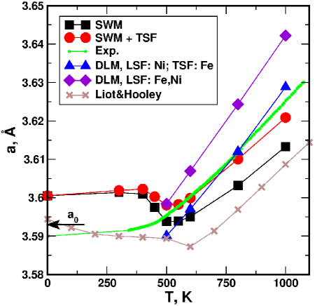
Figure 9: (Color online) Lattice constant of Fe₆₅Ni₃₅ obtained from the SWM total energy calculations (SWM) without and with the PDLM entropy (SWM + S^PDLM), from DLM calculations with LSF on Ni and TSF on Fe and LSF on both elements. The experimental data are taken from Ref. gorria09, . Liot and Hooley EMTO-CPA results from Ref. liot12, . The arrow ($a_{0}$) indicates the equilibrium lattice constant obtained in the FM state without zero point lattice vibration contribution.

As has been demonstrated in the previous section, one has also to account for the magnetic entropy contribution in quantitative analysis of the thermal lattice expansion in Fe-Ni alloys. Fortunately, it can be easily done within the SWM for the TSF since the magnitude of the magnetic moment entering (20) is just the average magnitude of the magnetic moment in the SWM calculations. Then the TSF magnetic entropy in the SWM in the presence of magnetic long- and short-range order can be determined using a PDLM-like single-site mean field approximation, which is consistent with the corresponding definition of the total energy in the SWM (see eq. (II)):

$$S^{\rm PDLM}=(1-s_{0})\sum_{i}c_{i}\ln(1+m_{i}).$$ (24)

Here, $s_{0}$ is the reduced magnetization, $c_{i}$ and $m_{i}$ are the concentration and local average magnetic moment of alloy component $i$. In Heisenberg systems with localized type of magnetism, the local magnetic moments are constant, but it is not the case of Fe-Ni alloys, and therefore they have been determined as the average over all the magnetic moments of spin-spirals except for $\mathbf{q}=0$ weighted according to the given MSRO.

Equation (24) does not account, however, for the MSRO. In an approximate way, it can be done by using $s_{0}=\xi_{1}$, i.e. the value of the spin-spin correlation function at the first coordination shell. This, at least, provides a smooth behavior of the entropy as a function of magnetic state near the Curie temperature.

The lattice constant of Fe₆₅Ni₃₅ with MSRO and TSF is shown in Fig. 9 (SWM + TSF). Although the account of the TSF improves the results for the lattice constant near the Curie temperature (500 K), still the lattice constant has a pronounced minimum in this region. The experimental lattice constant, in contrast, exhibits a very smooth temperature dependence with two different slopes below and above the Curie temperature. It is clear, that something is still missing in theory and this is most probably the LSF, the proper account of which can lift up the lattice constants in the paramagnetic region and eliminate the minimum at the Curie temperature.

The point is that the SWM results are in fact in good agreement with experimental data up to 400 K in the FM region, but shifted up by approximately 0.01 Å. In the paramagnetic region, this shift however disappears and the inclusion of the TSF helps but little. An additional shift can be obviously obtained from the LSF, which is obvious if one compares the DLM+LSF results with the DLM results by Liot and Hooley in Fig. 9. The LSF are small in the FM state and practically disappear with increasing magnetization. And vice versa, with decreasing magnetization, while approaching the magnetic transition, the role of the LSF increases. Therefore one can speculate that they are important in order to reproduce the smooth temperature dependence of the lattice constant in Fe₆₅Ni₃₅ near the Curie temperature.

Thus, both contributions, MSRO and LSF, are important for a quantitatively correct description of the thermal expansion in Fe-Ni alloys. The problem is, however, that it is not clear how to combine the LSF formalism with the SWM, which seems to be at the moment the only practical theoretical tool, which allows the inclusion of the MSRO effects in random alloys. Most probably, the solution requires the development of other types of techniques, which effectively combine these two finite temperature features of the itinerant magnets.

VII Summary

1. The spin-wave method is generalized here to the ferromagnetic state.

2. The developed SWM in combination with the CPA spin-spiral calculations is used then to calculate the contribution from the magnetic long- and short-range order to the total energy of the Fe₆₅Ni₃₅ Invar alloy.

3. The calculations show that the MSRO effects yield significant contribution to the temperature dependence of the lattice constant. In particular, they correct the PDLM-CPA results in the FM region up to 400 K, producing the thermal lattice expansion consistent with the experimental data.

4. The entropy contribution associated with the LSF and TSF has been considered in the ab initio modeling of the Invar effect. It provides quite significant shift of the lattice constant at high temperatures in the paramagnetic state, and should be considered in the accurate modeling of the thermal expansion in Fe-Ni alloys.

5. Although both the MSRO effect and LSF are important for accurate calculations of the equilibrium lattice constant of Fe-Ni alloys at elevated temperatures, it is practically impossible to include them together in the modeling within the used here theoretical techniques. This results in an abnormal behavior of the temperature dependence of the lattice constant close to the Curie temperature.

6. The magnetic transition temperature in the fcc Fe-Ni alloys is calculated taking the LSF on Ni into consideration. It is demonstrated that the LSF on Ni provide a substantial strengthening of the Ni-Ni and Fe-Ni magnetic exchange interactions in the paramagnetic state.

Appendix A Spin-spiral and noncollinear calculations by the EMTO-CPA method

The present implementation of noncollinear and spin-spiral calculations in the EMTO-CPA Green’s function method is done within the atomic sphere approximation where the magnetic configuration is site-projected, with the magnetic moment of a site given by the integrated magnetic density within the corresponding atomic sphere:

$$\mathbf{m}_{i}=\int_{\Omega_{i}}d\mathbf{r}\>\mathbf{m}(\mathbf{r}-\mathbf{R}_{i}).$$ (25)

Here, $\mathbf{m}(\mathbf{r}-\mathbf{R}_{i})$ is the magnetic density centred at site $i$ in position $\mathbf{R}_{i}$, and $\mathbf{m}_{i}$ is the magnetic moment of site $i$.

The magnetic configuration of the system is then given by polar angels $\theta_{i}$ and $\phi_{i}$ of the local magnetic moments $\mathbf{m}_{i}=m_{i}\,(\sin\theta_{i}\cos\phi_{i},\,\sin\theta_{i}\sin\phi_{i},\,\cos\theta_{i})$ of each site relative to the $z$-axis of the global frame of reference. If the local magnetic moment $m_{i}$ is defined in the local frame of reference along the local $z$ direction, it transforms to the global frame by the corresponding spin-$\frac{1}{2}$ rotation matrix:sandratskii98 ; mryasov91

$$\mathbf{U}_{i}=\begin{bmatrix}\cos(\theta_{i}/2)e^{i\phi_{i}/2}&\sin(\theta_{i}/2)e^{-i\phi_{i}/2}\\ \\ -\sin(\theta_{i}/2)e^{i\phi_{i}/2}&\cos(\theta_{i}/2)e^{-i\phi_{i}/2}\\ \end{bmatrix}$$ (26)

As has been demonstrated by Mryasov et al. mryasov91 , in the site-projected formalism, the electronic structure of a non-collinear system in the KKR or LMTO methods can be obtained using the local frame references of individual sites by the following transformation of the structure constants, or slope matrixandersen94 ; andersen98 in the case of the EMTO method:

$$\mathbf{\tilde{S}}^{ij}_{LL^{\prime}}=\mathbf{U}^{-1}_{i}\mathbf{S}^{ij}_{LL^{\prime}}\mathbf{U}_{j}.$$ (27)

Here, $\mathbf{S}^{ij}_{LL^{\prime}}=\mathbf{I}S^{ij}_{LL^{\prime}}$ and $S^{ij}_{LL^{\prime}}$ is the slope or structure constants matrix of the EMTO method and $\mathbf{I}$ is the unit matrix. Since $\mathbf{U}_{i}$ is unitary, $\mathbf{U}^{-1}_{i}=\mathbf{U}^{\dagger}_{i}$.

A similar formalism is valid in the case of spin-spiral calculations.mryasov91 Here, it is outlined for Bravais lattices in order to simplify notations, since its generalization to the multisite systems is straightforward. The spin spiral magnetic configuration for a fixed azimuth angle $\theta$ and wave vector $\mathbf{q}$ is determined by

$$\mathbf{m}_{i}=m_{i}\,\left(\sin\theta\cos(\mathbf{q}\mathbf{R}_{i}),\sin\theta\sin(\mathbf{q}\mathbf{R}_{i}),\cos\theta\right),$$ (28)

and the corresponding site projected spin rotation matrix (26) is obtained by substitution $\phi_{i}=\mathbf{q}\mathbf{R}_{i}$.

In the absence of the spin-orbit interaction, one can use the generalized Bloch theorem,sandratskii98 ; mryasov91 which allows one to disentangle the magnetic and crystal structures translational symmetries thereby reducing electronic structure calculations to the primitive unit cell of the underlying magnetic structure Bravais lattice. A spin spiral magnetic structure in this case is set up by the corresponding transformation of the structure constants (or slope matrixes). In particular, the structure constants or slope matrix for a spin-spiral with wave vector $\mathbf{q}$ and azimuth angle $\theta$ is

$$\mathbf{S}_{LL^{\prime}}(\mathbf{k})=$$ (29)

$$\mathbf{U}^{-1}\begin{bmatrix}S_{LL^{\prime}}(\mathbf{k}-\frac{\mathbf{q}}{2})&0\\ \\ 0&S_{LL^{\prime}}(\mathbf{k}+\frac{\mathbf{q}}{2})\\ \end{bmatrix}\mathbf{U},$$

where spin transformation matrix $U$ is given by (26) with $\phi=0$.

The potential function of the EMTO method, $\mathbf{D}_{L}(z)$,andersen94 ; andersen98 for particular energy $z$ and angular magnetic moments $L=(l,m)$ is obtained in the local frame of reference and thus it is a diagonal matrix in the spinor basis with ”spin-up” and ”spin-down” components: $D^{(\frac{1}{2})}_{L}(z)$ and $D^{(-\frac{1}{2})}_{L}(z)$. The path operator, whose poles are the electronic spectrum of the system and which is the main quantity for calculating electron density in the Green’s function formalism is then

$$\mathbf{g}_{LL^{\prime}}(\mathbf{k},z)=\frac{1}{\mathbf{S}_{LL^{\prime}}(\mathbf{k},z)-\mathbf{D}_{L}(z)}.$$ (30)

The above formalism is in fact straightforwardly generalized to the case of random alloys within the single-site coherent potential approximation. The path operator of the CPA effective medium is

$$\mathbf{\tilde{g}}_{LL^{\prime}}({\mathbf{k}},z)=\frac{1}{\mathbf{S}_{LL^{\prime}}({\mathbf{k}},z)-\mathbf{\tilde{D}}_{LL^{\prime}}(z)},$$ (31)

where $\mathbf{\tilde{g}}_{LL^{\prime}}({\mathbf{k}},z)$ and $\mathbf{\tilde{D}}_{LL^{\prime}}(z)$ are the path operator and potential function of the CPA effective medium, respectively. The latter is in general a non-diagonal matrix in the angular moment representation.

The CPA effective medium path operator and potential function are found from the set of CPA equationsCPA but in the spinor representation:

$$\mathbf{\widetilde{g}}_{LL^{\prime}}(z)=\int d{\mathbf{k}}\mathbf{\tilde{g}}_{LL^{\prime}}({\mathbf{k}},z)\equiv\mathbf{\widetilde{g}}$$ (32)

$$\mathbf{g}^{\alpha}=\mathbf{\widetilde{g}}+\mathbf{\widetilde{g}}\left[\mathbf{D}^{\alpha}-\mathbf{\tilde{D}}\right]\mathbf{g}^{\alpha}$$ (33)

$$\mathbf{\widetilde{g}}=\sum_{\alpha}c^{\alpha}\mathbf{g}^{\alpha}.$$ (34)

Here, $c^{\alpha}$, $\mathbf{D}^{\alpha}$, and $\mathbf{g}^{\alpha}$ are the concentration, potential function and on-site path operator of alloy component $\alpha$ in the CPA effective medium. Both, $\mathbf{D}^{\alpha}$ and $\mathbf{g}^{\alpha}$, are digonal in the spinor representation and therefore the rest of the formalism for the self-consistent and total energy calculations is similar to the one for the collinear EMTO-CPA method.vitos01

Appendix B Details of the spin-wave method calculations

The total energy of a system in magnetic configuration $\alpha$, specified by its long-range order parameter, $s_{0}^{\alpha}$, and spin-spin correlation functions, $\xi^{\rm SRO}_{\alpha}(\mathbf{R})$ or $\xi^{\rm SRO}_{\alpha}(\mathbf{q})$, is given by (II). In the actual spin-wave calculations, when the Monkohrst-Packmonkhorst72 q-point grid is used, the total energy of the system in magnetic state $\alpha$ for a particular volume per atom, $\Omega$, is

$$E^{\alpha}(\Omega) = s_{0}^{\alpha}E(\mathbf{q}=0,\Omega)+$$

$$\sum_{i}w_{i}E(\mathbf{q}_{i},\Omega)\left[1-s_{0}^{\alpha}+\xi^{\rm SRO}_{\alpha}(\mathbf{q}_{i})\right],$$

where $\mathbf{q}_{i}$ and $w_{i}$ are the q-points of the grid and their weights. $E(\mathbf{q}_{i},\Omega)$ is the total energy of a system for a planar spin-spiral ($\theta=\pi/2$) with wave vector $\mathbf{q}_{i}$ and volume per atom $\Omega$. $E(\mathbf{q}=0,\Omega)$ is the energy of the ferromagnetic state (point $\mathbf{q}=0$ can be in the grid or calculated separately).

Thus, the set of the total energies $E(\mathbf{q}_{i},\Omega)$ on the q-point grid uniquely defines the total energy of the system in any given magnetic configuration $\alpha$, $E^{\alpha}(\Omega)$. The accuracy of such a representation of a particular magnetic state can be always checked for the given grid of q-points by calculating $\xi^{\rm SRO}_{\alpha}(\mathbf{R})$ from $\xi^{\rm SRO}_{\alpha}(\mathbf{q}_{i})$.ruban12 Although, obviously, there always be a problem with $\xi^{\rm SRO}_{\alpha}(\mathbf{R})$ for $R\to\infty$ when the finite grid is used, in most cases it cannot affect the result for the total energy due to the relatively short-range character of the magnetic exchange interactions, which is in particular the case of Fe-Ni alloys, where the the 7$\times$7$\times$7 Monkhorst-Pack grid provides quite accurate total energies for the whole range of magnetic states.

- (1) C. E. Guillaume, C. R. Acad. Sci. 125, 235 (1897).
- (2) In the Materials Science and Engineering literature weight % are usually used without mentioning. Close to the Invar composition, wt. % of Ni is about 1 % higher than atomic %.
- (3) For instance, the much lower thermal expansion coefficient at room temperature can be obtained using Co additions, like in the case of super Invar alloy, Fe63Ni31Co6.
- (4) Charles-Edouard Guillaume - Nobel Lecture: Invar and Elinvar. Nobelprize.org. Nobel Media AB 2014. Web. 1 Nov 2016. (http://www.nobelprize.org/nobel_prizes/physics/ laureates/1920/guillaume-lecture.html) (or C. E. Guillaume, in Nobel Lectures in Physics 1901-1921 (Elsevier, Amsterdam, 1967).
- (5) R. J. Weiss, Proc. R. Soc. London A 82, 281 (1963).
- (6) W. Peperhoff and M. Acet, Constitution and magnetism of Iron and its Alloys (Springer-Verlag, Berlin, Heidelberg, New York, 2001).
- (7) V. L. Moruzzi, Phys. Rev. B 41, 6939 (1990).
- (8) M. Podgorny, Phys. Rev. B 46, 6293 (1992).
- (9) P. Mohn, K. Schwarz and D. Wagner, Phys. Rev. B 43, 3318 (1991).
- (10) P. Entel, E. Hoffmann, P. Mohn, K. Schwarz, and V. L. Moruzzi, Phys. Rev. B 47, 8706 (1993).
- (11) M. Schröter, H. Ebert, H. Akai, P. Entel, E. Hoffmann, and G. G. Reddy, Phys. Rev. B 52, 188 (1995).
- (12) P. Entel, E. Hoffmann, M. Clossen, K. Kadau, M. Schröter, R. Meyer, H. C. Herper, and M. S. Yang, in The Invar Effect: A Centennial Symposium, ed. by J. Wittenauer (The Minerals, Metals and Materials Society, Warrendale, 1997) p.87.
- (13) Y. Kakehashi, J. Phys. Soc. Japan 50, 2236 (1981).
- (14) Y. Kakehashi, Physica B 161, 143 (1989).
- (15) D. D. Johnson, F. J. Pinski, J. B. Staunton, B. L. Gyorffy, and G. M. Stocks, in Physical Metallurgy of Controlled Expansion Invar-type alloys (ed. K. C. Russel and D. F. Smith) p.3 (The Minerals, Metals & Materials Society, 1990).
- (16) D. D. Johnson, and W. A. Shelton, in The Invar Effect: a Centennial Simposium, ed. by J. Wittenauer (The Minerals, Metals and Materials Society, Warrendale, 1997) p.63.
- (17) In the DLM approach, the paramagnetic state is modeled by a random alloy of spin-up and spin-down magnetic moment orientations of every component of the system. For details, see B. L. Gyorffy, A.J. Pindor, J. Staunton, G. M. Stocks, and H.Winter, J. Phys. F 15, 1337 (1985).
- (18) H. Akai, and P. H. Dederichs, Phys. Rev. B 47, 8739 (1993).
- (19) V. Crisan, P. Entel, H. Ebert, H. Akai, D. D. Johnson, and J. B. Staunton, Phys. Rev B 66, 014416 (2002).
- (20) A. V. Ruban, S. Khmelevskyi, P. Mohn, and B. Johansson, Phys. Rev. B 76, 014420 (2007).
- (21) S. Khmelevskyi, I. Turek, and P. Mohn, Phys. Rev. Lett. 91, 037201 (2003).
- (22) S. Khmelevskyi, and P. Mohn, Phys. Rev. B 69, 140404 (2004).
- (23) S. Khmelevskyi, I. Turek, and P. Mohn, Phys. Rev. B 70, 132401 (2004)
- (24) S. Khmelevskyi, A. V. Ruban, Y. Kakehashi, P. Mohn, B. Johansson, Phys. Rev. B 72, 064510 (2005).
- (25) F. Liot Thermal Expansion and Local Environment Effects in Ferromagnetic Iron-Based Alloys: A Theoretical Study, PhD dissertation (Link?oping: Link?oping University Electronic Press, 2009).
- (26) F. Liot and C. A. Hooley, Numerical Simulations of the Invar Effect in Fe-Ni, Fe-Pt, and Fe-Pd Ferromagnets, 2012 (arXiv:1208.2850).
- (27) F. Liot, Magnetization, magnetostriction, and their relationship in Invar Fe1-xAx (A = Pt,Ni), 2014 (arXiv:1401.6089).
- (28) V. L. Moruzzi, J. F. Janak, and K. Schwarz, Phys. Rev. B 37, 790 (1988).
- (29) A. V. Ruban, V. I. Razumovskiy, Phys. Rev. B 85, 174407 (2012).
- (30) P. A. Korzhavyi, A. V. Ruban, S. I. Simak, and Yu. Kh. Vekilov, Phys. Rev. B 49, 14229 (1994).
- (31) S. V. Halilov, H. Eschrig, A. Y. Perlov, and P. M. Oppeneer, Phys. Rev. B 58, 293 (1998).
- (32) L. M. Sandratskii, Adv. Phys. 47, 91 (1998).
- (33) J. L. Robertson, G. E. Ice, C. J. Sparks, X. Jiang, P. Zschack, F. Bley, S. Lefebvre, and M. Bessiere, Phys. Rev. Lett. 82, 2911 (1999).
- (34) Y. Tsunoda, L. Hao, S. Shimomura, F. Ye, J. L. Robertson, J. Fernandez-Baca, Phys. Rev. B 78, 094105 (2008).
- (35) P. Soven, Phys. Rev. B 156, 809 (1967); B. L. Gyorffy, Phys. Rev. B 5, 2382 (1972).
- (36) O.K. Andersen, O. Jepsen, and G. Krier in Lectures on Methods of Electronic Structure Calculations, edited by V. Kumar, O.K. Andersen, and A. Mookerjee (World Scientific Publishing Co., Singapore, 1994), pp. 63-124.
- (37) O. K. Andersen, C. Arcangeli, R. W. Tank, T. Saha-Dasgupta, G. Krier, O. Jepsen, and I. Dasgupta, in Mat. Res. Soc. Symp. Proc. 491, pp. 3-34 (1998).
- (38) L. Vitos, Phys. Rev. B 64, 014107 (2001); L. Vitos, I. A. Abrikosov, B. Johansson, Phys. Rev. Lett. 87 156401 (2001).
- (39) A. V. Ruban, H. L. Skriver, Phys. Rev. B 66, 024201 (2002); A. V. Ruban, S. I. Simak, P. A. Korzhavyi, and H. L. Skriver, Phys. Rev. B 66, 024202 (2002).
- (40) I. A. Abrikosov, S. I. Simak, B. Johansson, A. V. Ruban, and H. L. Skriver, Phys. Rev. B 56, 9319 (1997).
- (41) O. E. Peil, A. V. Ruban, and B. Johansson, Phys. Rev. B 85, 165140 (2012).
- (42) H. J. Monkhorst and J. D. Pack, Phys. Rev. B 13, 5188 (1972).
- (43) J. P. Perdew and Y. Wang, Phys. Rev. B 45, 13244 (1992).
- (44) J. P. Perdew, K. Burke, and M. Ernzerhof, Phys. Rev. Lett., 77, 3865 (1996).
- (45) F. Liot, I. A. Abrikosov, Phys. Rev. B 79, 014202 (2009).
- (46) The choice of the alloy composition, Fe62.5Ni37.5, was dictated by the optimization of the supercell size under constrain having the first eight pair correlation functions as small as possible, i.e. to represent best a random alloy up to the 8th coordination shell. Let us note, that this alloy composition is still in the Invar region.
- (47) P. E. Blöchl, Phys. Rev. B 50, 17953 (1994).
- (48) G. Kresse, D. Joubert, Phys. Rev. B 59, 1758 (1999).
- (49) G. Kresse, J. Hafner, Phys. Rev. B 47, 558 (1993).
- (50) G. Kresse, J. Hafner, Phys. Rev. B 49, 14251 (1994).
- (51) G. Kresse, J. Furthműller, Phys. Rev. B 54, 11169 (1996).
- (52) A. V. Ruban, S. Khmelevskyi, P. Mohn, and B. Johansson, Phys. Rev. B 75, 054402 (2007).
- (53) A. V. Ruban, M. I. Katsnelson, W. Olovsson, S. I. Simak, and I. A. Abrikosov, Phys. Rev. B 71, 054402 (2005).
- (54) A. V. Ruban, A. B. Belonoshko, and N. V. Skorodumova, Phys. Rev. B 87, 014405 (2013).
- (55) L. M. Sandratskii, Phys. Rev. B 78, 094425 (2008).
- (56) P. A. Korzhavyi, private communication.
- (57) J. Crange and G. C. Hallam, Proc. Royal Soc. A 272, 119 (1963).
- (58) A. I. Liechtenstein, M. I. Katsnelson, V. P. Antropov, and V. A. Gubanov, J. Magn. Magn. Mater. 200, 148 (1987).
- (59) A. V. Ruban, M. Dehghani, Phys. Rev. B 94, 104111 (2016).
- (60) Let us note, that the GGA also increases the magnitude of the magnetic moment compared to the LDA, and the GGA exchange interaction will produce higher Curie temperatures by approximately 150 K (see, for instance, Ref. ruban04, ).
- (61) M. Hayase, M. Shiga, and Y. Nakamura, J. Phys. Soc. Jap. 34, 925 (1973).
- (62) A. V. Ruban, S. Shallcross, S. I. Simak, and H. L. Skriver Phys. Rev. B 70, 125115 (2004).
- (63) A. V. Ruban, P. A. Korzhavyi, and B. Johansson, Phys. Rev. B 77, 094436 (2008).
- (64) P. Gorria, D. Martinez-Blanco, M.J. Perez, J.A. Blanco, A. Hernando, M.A. Laguna-Marco, D. Haskel, N. Souza-Neto, R.I. Smith, W.G. Marshall, G. Garbarino, M. Mezouar, A. Fernandez-Martinez, J. Chaboy, L. FernandezBarquin, J.A. RodriguezCastrillon, M. Moldovan, J.I. GarciaAlonso, J. Zhang, A. Llobet, J.S. Jiang, Phys. Rev. B 80, 064421 (2009).
- (65) O. N. Mryasov, A. I. Liechtenstein, L. M. Sandratskii, and V. A. Gubanov, J. Phys.: Condens. Matter 3, 7683 (1991).