Feasible superadiabatic-based shortcuts for fast generating 3D entanglement between two atoms

Abstract

Abstract We propose a scheme to realize fast generation of three-dimensional entanglement between two atoms via superadiabatic-based shortcuts in an atom-cavity-fiber system. The scheme is experimentally feasible because of the same form of the counterdiabatic Hamiltonian as that of the effective Hamiltonian. Besides, numerical simulations are given to prove that the scheme is strongly robust against variations in various parameters and decoherence.
Keywords: 3D entanglement, Shortcuts to adiabaticity, Superadiabatic iterations

I Introduction

With the rapid development in quantum information processing, high-dimensional entanglement is increasingly drawing attention of researchers due to its more superior security than qubit entanglement in the field of quantum key distribution and its greater violation of local realism BKB2001 ; BM2002 ; CBK2002 ; YW2016 ; DPMW2000 . Thus, the generation of high-dimensional entanglement is of great importance. Up to present, a large number of schemes have been proposed for generating high-dimensional entanglement via various techniques XHL2010 ; LP2012 ; YLS2015 ; SSW2016 ; WG2011 ; SJR2013 ; QCW2013 ; XQ201402 ; SL2014 ; DJC2015 . Among these techniques, stimulated Raman adiabatic passage (STIRAP) is widely used in fields of time-dependent interaction for many purposes KHB1998 ; PIM2007 because of its robustness against atomic spontaneous emissions and variations in experimental parameters. However, STIRAP usually requires a relatively long interaction time for restraining non-adiabatic transitions.

A set of techniques called “Shortcuts to adiabaticity (STA)” are promising for quantum information processing which actually fights against the decoherence, noise, or losses that are accumulated during a long operation time. Hence, many schemes are proposed to construct STA XCA2010 ; XASA2010 ; SIX2012 ; dC2012 ; ARXD2012 ; SMG2013 ; AC2013 ; ETS2013 ; DGO2014 ; YHC2016 ; AHA2016 . By using STA, a great deal of remarkable achievements have been made in quantum information processing MYLJ2014 ; YHC2014 ; XL2015 ; JTD2015 ; YLQ2015 ; XHQ2016 . Also, numerous schemes have been come up with for fast generating high-dimensional entanglement JYC2016 ; ZYY2016 ; WSJ2016 ; HSW2016 ; WJZ2016 , in which Chen $et~{}al$ and He $et~{}al$ prepared a three-atom singlet state ZYY2016 and a two-atom 3D entangled state HSW2016 , respectively, by using transitionless quantum driving (TQD); Lin $et~{}al$ JYC2016 and Wu $et~{}al$ WSJ2016 implemented two-atom 3D entangled states, respectively, based on Lewis-Riesenfeld invariants (LRI); Wu $et~{}al$ also generated three-atom tree-type 3D entangled states with both of TQD and LRI WJZ2016 .

In this work, we propose a superadiabatic scheme for fast generating two-atom 3D entanglement via superadiabatic iterations. Superadiabatic iterations as an extension of the traditional adiabatic approximation was introduced in BERRY1987 . The technique was adopted for speeding up adiabatic process first by Ibáñez $et~{}al$ SIX2012 ; SXJ2013 . A short time before, Song $et~{}al$ extended it to a three-level system XQJ2016 . More recently, Huang $et~{}al$ HCW2016 and Kang YYQ2016 generated Greenberger–Horne–Zeilinger state and $W$ state, respectively, by using this technique. Now we apply this technique to the fast generation of two-atom 3D entanglement. Apart from the rapid rate, we implement two-atom 3D entanglement with pretty high fidelity. More importantly, as the second iteration different from the first iteration (i.e., TQD), the superadiabatic scheme does not need an additional coupling between the initial and finial states, and the same form of counterdiabatic Hamiltonian as that of effective Hamiltonian guarantees its high feasibility in experiment.

This paper is structured as follows: The physical model and effective dynamics are shown in section 2. In section 3, we give the superadiabatic scheme for fast generating 3D entanglement between two atoms. In section 4, numerical simulation results prove that the scheme is fast, valid and robust. The conclusion is given in section 5.

II Physical model and effective dynamics

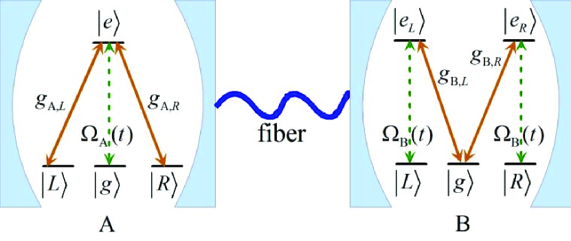
Figure 1: The diagrammatic sketch of the atom-cavity-fiber system, atomic level configurations and related transitions.

The schematic sketch of the physical model for fast generating two-atom 3D entanglement is shown in figure 1. There are two atoms trapped, respectively, in two spatially separated bimodule cavities connected by a fiber which satisfies the short fiber limit to ensure that only resonant modes of the fiber interact with cavity modes SMB2006 . Two atoms both have three ground states $|L\rangle$, $|g\rangle$ and $|R\rangle$. In addition, atom A has one excited state $|e\rangle$ and atom B has two excited states $|e_{L}\rangle$ and $|e_{R}\rangle$. Atomic transitions $|e\rangle_{\rm A}\leftrightarrow|L(R)\rangle_{\rm A}$ and $|e_{L(R)}\rangle_{\rm B}\leftrightarrow|g\rangle_{\rm B}$ are resonantly coupled to the left(right)-circularly polarized modes of cavity A and cavity B, respectively, with corresponding coupling constants $g_{{\rm A},{L(R)}}$ and $g_{{\rm B},{L(R)}}$. Transitions $|e\rangle_{\rm A}\leftrightarrow|g\rangle_{\rm A}$ and $|e_{L(R)}\rangle_{\rm B}\leftrightarrow|L(R)\rangle_{\rm B}$ are resonantly driven by classical laser fields, respectively, with Rabi frequencies $\Omega_{\rm A}(t)$ and $\Omega_{\rm B}(t)$. Then, the interaction Hamiltonian of the atom-cavity-fiber system is ($\hbar=1$):

$$H(t) = \Omega_{\rm A}(t)|g\rangle_{\rm A}\langle{e}|+\sum_{i=L,R}[\Omega_{\rm B}(t)|i\rangle_{\rm B}\langle{e_{i}}|+g_{{\rm A},i}a_{{\rm A},i}|e\rangle_{\rm A}\langle{i}|$$ (1)

$$+g_{{\rm B},i}a_{{\rm B},i}|e_{i}\rangle_{\rm B}\langle{g}|+vb_{i}(a_{{\rm A},i}^{\dagger}+a_{{\rm B},i}^{\dagger})]+\rm H.c.,$$

where $a_{{\rm A(B)},L(R)}$ and $b_{L(R)}$ is the annihilation operator of left(right)-circularly polarized mode of cavity A(B) and the fiber, respectively; $v$ is the coupling strength between the two cavities and the fiber. For convenience, we assume $g_{{\rm A(B)},L(R)}$ is real, $g_{{\rm A},{L}}=g_{{\rm A},{R}}=g_{\rm A}$ and $g_{{\rm B},{L}}=g_{{\rm B},{R}}=g_{\rm B}$.

If the initial state of the whole system is $|\phi_{1}\rangle=|g\rangle_{\rm A}|g\rangle_{\rm B}|0\rangle_{c\rm A}|0\rangle_{f}|0\rangle_{c\rm B}$ denoting two atoms both in state $|g\rangle$ and two cavities and the fiber all in the vacuum state, Hamiltonian (1) can be rewritten by

$$H(t) = \Omega_{\rm A}(t)|\phi_{1}\rangle\langle\phi_{2}|+g_{\rm A}|\phi_{2}\rangle(\langle\phi_{3}|+\langle\phi_{4}|)+v(|\phi_{3}\rangle\langle\phi_{5}|+|\phi_{4}\rangle\langle\phi_{6}|+|\phi_{5}\rangle\langle\phi_{7}|+|\phi_{6}\rangle\langle\phi_{8}|)$$ (2)

$$+g_{\rm B}(|\phi_{7}\rangle\langle\phi_{9}|+|\phi_{8}\rangle\langle\phi_{10}|)+\Omega_{\rm B}(t)(|\phi_{9}\rangle\langle\phi_{11}|+|\phi_{10}\rangle\langle\phi_{12}|)+\rm H.c.,$$

for which

$$|\phi_{1}\rangle=|g\rangle_{\rm A}|g\rangle_{\rm B}|0\rangle_{c\rm A}|0\rangle_{f}|0\rangle_{c\rm B},\quad|\phi_{2}\rangle=|e\rangle_{\rm A}|g\rangle_{\rm B}|0\rangle_{c\rm A}|0\rangle_{f}|0\rangle_{c\rm B},$$

$$|\phi_{3}\rangle=|L\rangle_{\rm A}|g\rangle_{\rm B}|L\rangle_{c\rm A}|0\rangle_{f}|0\rangle_{c\rm B},\quad|\phi_{4}\rangle=|R\rangle_{\rm A}|g\rangle_{\rm B}|R\rangle_{c\rm A}|0\rangle_{f}|0\rangle_{c\rm B},$$

$$|\phi_{5}\rangle=|L\rangle_{\rm A}|g\rangle_{\rm B}|0\rangle_{c\rm A}|L\rangle_{f}|0\rangle_{c\rm B},\quad|\phi_{6}\rangle=|R\rangle_{\rm A}|g\rangle_{\rm B}|0\rangle_{c\rm A}|R\rangle_{f}|0\rangle_{c\rm B},$$

$$|\phi_{7}\rangle=|L\rangle_{\rm A}|g\rangle_{\rm B}|0\rangle_{c\rm A}|0\rangle_{f}|L\rangle_{c\rm B},\quad|\phi_{8}\rangle=|R\rangle_{\rm A}|g\rangle_{\rm B}|0\rangle_{c\rm A}|0\rangle_{f}|R\rangle_{c\rm B},$$

$$|\phi_{9}\rangle=|L\rangle_{\rm A}|e_{L}\rangle_{\rm B}|0\rangle_{c\rm A}|0\rangle_{f}|0\rangle_{c\rm B},\quad|\phi_{10}\rangle=|R\rangle_{\rm A}|e_{R}\rangle_{\rm B}|0\rangle_{c\rm A}|0\rangle_{f}|0\rangle_{c\rm B},$$

$$|\phi_{11}\rangle=|L\rangle_{\rm A}|L\rangle_{\rm B}|0\rangle_{c\rm A}|0\rangle_{f}|0\rangle_{c\rm B},\quad|\phi_{12}\rangle=|R\rangle_{\rm A}|R\rangle_{\rm B}|0\rangle_{c\rm A}|0\rangle_{f}|0\rangle_{c\rm B}.$$ (3)

$|L(R)\rangle$ denotes a single left(right)-circularly polarized photon state. Now we set a set of orthogonal states

$$|\psi_{k}\rangle=\frac{1}{\sqrt{2}}(|\phi_{2k+1}\rangle+|\phi_{2k+2}\rangle),\quad|\psi_{k}^{-}\rangle=\frac{1}{\sqrt{2}}(|\phi_{2k+1}\rangle-|\phi_{2k+2}\rangle),$$ (4)

with $k=1,2,3,4,5$. Then Hamiltonian (2) becomes

$$H(t) = \Omega_{\rm A}(t)|\phi_{1}\rangle\langle\phi_{2}|+\sqrt{2}g_{\rm A}|\phi_{2}\rangle\langle\psi_{1}|+g_{\rm B}(|\psi_{3}\rangle\langle\psi_{4}|+|\psi_{3}^{-}\rangle\langle\psi_{4}^{-}|)$$ (5)

$$+v(|\psi_{1}\rangle\langle\psi_{2}|+|\psi_{1}^{-}\rangle\langle\psi_{2}^{-}|+|\psi_{2}\rangle\langle\psi_{3}|+|\psi_{2}^{-}\rangle\langle\psi_{3}^{-}|)$$

$$+\Omega_{\rm B}(t)(|\psi_{4}\rangle\langle\psi_{5}|+|\psi_{4}^{-}\rangle\langle\psi_{5}^{-}|)+\rm H.c..$$

Because $|\psi_{k}^{-}\rangle$ will not be involved during the whole evolution if $|\phi_{1}\rangle$ is the initial state, so Hamiltonian (5) becomes

$$H(t) = \Omega_{\rm A}(t)|\phi_{1}\rangle\langle\phi_{2}|+\sqrt{2}g_{\rm A}|\phi_{2}\rangle\langle\psi_{1}|+v(|\psi_{1}\rangle\langle\psi_{2}|+|\psi_{2}\rangle\langle\psi_{3}|)$$ (6)

$$+g_{\rm B}|\psi_{3}\rangle\langle\psi_{4}|+\Omega_{\rm B}(t)|\psi_{4}\rangle\langle\psi_{5}|+\rm H.c..$$

Next, for further simplification, we set $\sqrt{2}g_{\rm A}=v=g_{\rm B}=g$ and rewrite Hamiltonian (6) as

$$H(t) = H_{0}+V(t),$$

$$H_{0} = g(|\Psi_{1}^{+}\rangle\langle\Psi_{1}^{+}|-|\Psi_{1}^{-}\rangle\langle\Psi_{1}^{-}|)+\sqrt{3}g(|\Psi_{2}^{+}\rangle\langle\Psi_{2}^{+}|-|\Psi_{2}^{-}\rangle\langle\Psi_{2}^{-}|),$$

$$V(t) = \frac{\Omega_{\rm A}(t)}{\sqrt{3}}|\phi_{1}\rangle[\langle\Psi_{d}|-\frac{\sqrt{3}}{2}(\langle\Psi_{1}^{+}|+\langle\Psi_{1}^{-}|)+\frac{1}{2}(\langle\Psi_{2}^{+}|+\langle\Psi_{2}^{-}|)]$$ (7)

$$+\frac{\Omega_{\rm B}(t)}{\sqrt{3}}[|\Psi_{d}\rangle+\frac{\sqrt{3}}{2}(|\Psi_{1}^{+}\rangle+|\Psi_{1}^{-}\rangle)+\frac{1}{2}(|\Psi_{2}^{+}\rangle+|\Psi_{2}^{-}\rangle)]\langle\psi_{5}|+\rm H.c.,$$

with the following transformations

$$|\Psi_{d}\rangle=\frac{1}{\sqrt{3}}(|\phi_{2}\rangle-|\psi_{2}\rangle+|\psi_{4}\rangle),\quad|\Psi_{1}^{\pm}\rangle=-\frac{1}{2}[|\phi_{2}\rangle\pm(|\psi_{1}\rangle-\psi_{3}\rangle)-|\psi_{4}\rangle],$$

$$|\Psi_{2}^{\pm}\rangle=\frac{1}{2\sqrt{3}}[|\phi_{2}\rangle+2|\psi_{2}\rangle\pm\sqrt{3}(|\psi_{1}\rangle+\psi_{3}\rangle)+|\psi_{4}\rangle].$$ (8)

Then after performing the unitary transformation $U=\exp(-iH_{0}t)$ and neglecting high oscillating terms under the limit condition $\Omega_{\rm A(B)}(t)\ll 2g$, we simplify Hamiltonian (II) to an effective Hamiltonian

$$H_{e}(t)=\Omega_{1}(t)|\phi_{1}\rangle\langle\Psi_{d}|+\Omega_{2}(t)|\Psi_{d}\rangle\langle\psi_{5}|+\rm H.c.,$$ (9)

with $\Omega_{1}(t)=\Omega_{\rm A}(t)/\sqrt{3}$ and $\Omega_{2}(t)=\Omega_{\rm B}(t)/\sqrt{3}$.

III Superadiabatic scheme for fast generating two-atom 3D entanglement

Instantaneous eigenstates of Hamiltonian (9) with eigenvalues $\eta_{\pm}=\pm\Omega(t)$ and $\eta_{0}=0$, respectively, are

$$|n_{\pm}(t)\rangle = \frac{1}{\sqrt{2}}[\sin\theta_{0}(t)|\phi_{1}\rangle{\pm}|\Psi_{d}\rangle+\cos\theta_{0}(t)|\psi_{5}\rangle],$$

$$|n_{0}(t)\rangle = \cos\theta_{0}(t)|\Psi_{1}\rangle-\sin\theta_{0}(t)|\Psi_{2}\rangle,$$ (10)

where $\Omega(t)=\sqrt{\Omega_{1}(t)^{2}+\Omega_{2}(t)^{2}}$ and $\tan\theta_{0}(t)=\Omega_{1}(t)/\Omega_{2}(t)$. We transform $H_{e}(t)$ to the adiabatic frame by performing the unitary transformation $U_{0}(t)=\sum_{k=\pm,0}|n^{\prime}_{k}\rangle\langle n_{k}(t)|$. At each instant in time, $U_{0}(t)$ maps the adiabatic eigenstate $n_{k}(t)$ onto the time-independent state $|n^{\prime}_{k}\rangle$. In the adiabatic frame, the Hamiltonian (9) becomes

$$H_{1}(t) = U_{0}(t)H_{e}(t)U_{0}^{\dagger}(t)+i\dot{U}_{0}(t)U_{0}^{\dagger}(t)$$ (11)

$$= \Omega(t)[|n^{\prime}_{+}\rangle\langle n^{\prime}_{+}|-|n^{\prime}_{-}\rangle\langle n^{\prime}_{-}|]+\frac{\dot{\theta}_{0}(t)}{\sqrt{2}}[i|n^{\prime}_{+}\rangle\langle n^{\prime}_{0}|+i|n^{\prime}_{-}\rangle\langle n^{\prime}_{0}|+\rm H.c.].$$

The effective system evolution will adiabatically follow one of states $\{|n^{\prime}_{0,\pm}\rangle\}$ with adiabatic approximation $|\dot{\theta}_{0}(t)|\ll\sqrt{2}\Omega(t)$ which needs very long runtime. For shortening runtime, Demirplack and Rice DR and Berry MVB2009 proposed that adding a suitable counterdiabatic (CD) Hamiltonian $H_{\rm CD}(t)$ to the original Hamiltonian can suppress transitions between different eigenstates. In the adiabatic frame CD Hamiltonian may be $-i\dot{U}_{0}(t)U_{0}^{\dagger}(t)$, which is written in $\{|\phi_{1}\rangle,|\Psi_{d}\rangle,|\psi_{5}\rangle\}$ frame by

$$H_{\rm CD}^{(1)}(t)=-iU_{0}^{\dagger}(t)\dot{U}_{0}(t)=i\dot{\theta}_{0}(t)(|\phi_{1}\rangle\langle\psi_{5}|-|\psi_{5}\rangle\langle\phi_{1}|).$$ (12)

CD Hamiltonian (12) needs a direct coupling between $|\phi_{1}\rangle$ and $|\psi_{5}\rangle$, which is too hard to implement in practice for such a complex system.

Superadiabatic states (instantaneous eigenstates of $H_{1}(t)$) with eigenvalues $\eta^{\prime}_{\pm}=\pm\Omega^{\prime}(t)$ and $\eta^{\prime}_{0}=0$, respectively, are

$$|n^{\prime\prime}_{\pm}(t)\rangle = \frac{1}{{2}}\{i[1\pm\cos\theta_{1}(t)]|n^{\prime}_{+}\rangle\pm\sqrt{2}\sin\theta_{1}(t)|n^{\prime}_{0}\rangle+i[1\mp\cos\theta_{1}(t)]|n^{\prime}_{-}\rangle\},$$

$$|n^{\prime\prime}_{0}(t)\rangle = \frac{1}{\sqrt{2}}[-i\sin\theta_{1}(t)|n^{\prime}_{+}\rangle+\sqrt{2}\cos\theta_{1}(t)|n^{\prime}_{0}\rangle+i\sin\theta_{1}(t)|n^{\prime}_{-}\rangle],$$ (13)

for which $\Omega^{\prime}(t)=\sqrt{\dot{\theta}_{0}(t)^{2}+\Omega(t)^{2}}$ and $\tan\theta_{1}(t)=\dot{\theta}_{0}(t)/\Omega(t)$. Then we transform $H_{1}(t)$ to the superadiabatic frame by the unitary transformation $U_{1}(t)=\sum_{k=\pm,0}|\widetilde{n}_{k}\rangle\langle n^{\prime\prime}_{k}(t)|$. Analogous to the adiabatic CD Hamiltonian (12), the superadiabatic CD Hamiltonian $-i\dot{U}_{1}(t)U_{1}^{\dagger}(t)$ is written in $\{|\phi_{1}\rangle,|\Psi_{d}\rangle,|\psi_{5}\rangle\}$ frame by

$$H_{\rm CD}^{(2)}(t) = -iU_{0}^{\dagger}(t)U_{1}^{\dagger}(t)\dot{U}_{1}(t)U_{0}(t)$$ (14)

$$= \dot{\theta}_{1}(t)[-\cos\theta_{0}(t)|\phi_{1}\rangle\langle\Psi_{d}|+\sin\theta_{0}(t)|\Psi_{d}\rangle\langle\psi_{5}|]+\rm H.c..$$

$H_{\rm CD}^{(2)}(t)$ is satisfactory because it has the same form as the effective Hamiltonian (9).

We regard $\Omega^{\prime}_{1}(t)=-\dot{\theta}_{1}(t)\cos\theta_{0}(t)$ and $\Omega^{\prime}_{2}(t)=\dot{\theta}_{1}(t)\sin\theta_{0}(t)$ as two auxiliary pulses added to the pulses $\Omega_{1}(t)$ and $\Omega_{2}(t)$, respectively. Then modified pulses $\Omega^{\prime\prime}_{1}(t)=\Omega_{1}(t)+\Omega^{\prime}_{1}(t)$ and $\Omega^{\prime\prime}_{2}(t)=\Omega_{2}(t)+\Omega^{\prime}_{2}(t)$ can drive the effective system to evolve along one of the superadiabatic state in equation (III). Therefore, if related parameters meet time boundary conditions $\{\theta_{1}(0)=\theta_{1}(t_{f})=0,\theta_{0}(0)=0,\theta_{0}(t_{f})=-\arctan\sqrt{2}\}$ ($t_{f}$ is the final time), $|n^{\prime\prime}_{0}(t)\rangle$ will act as a medium state for achieving the expected transformation $|\phi_{1}\rangle\rightarrow\frac{1}{\sqrt{3}}(|\phi_{1}\rangle+\sqrt{2}|\psi_{5}\rangle)$. By this way, we obtain the 3D entanglement between two atoms in the superadiabatic scheme

$$|\Psi_{\rm 3D}\rangle = \frac{1}{\sqrt{3}}(|\phi_{1}\rangle+|\phi_{11}\rangle+|\phi_{12}\rangle)$$ (15)

$$= \frac{1}{\sqrt{3}}(|g\rangle_{\rm A}|g\rangle_{\rm B}+|L\rangle_{\rm A}|L\rangle_{\rm B}+|R\rangle_{\rm A}|R\rangle_{\rm B})\otimes|0\rangle_{c\rm A}|0\rangle_{f}|0\rangle_{c\rm B}.$$

IV Numerical simulations

For meeting $\{\theta_{1}(0)=\theta_{1}(t_{f})=0,\theta_{0}(0)=0,\theta_{0}(t_{f})=-\arctan\sqrt{2}\}$, we choose $\Omega_{2}(t)$ and $\Omega_{1}(t)$ as NTB2001

$$\Omega_{2}(t) = \frac{1}{\sqrt{3}}\Omega_{0}\exp[-(t-t_{f}/2-t_{0})^{2}/t_{c}^{2}]+\Omega_{0}\exp[-(t-t_{f}/2+t_{0})^{2}/t_{c}^{2}],$$

$$\Omega_{1}(t) = -\frac{\sqrt{2}}{\sqrt{3}}\Omega_{0}\exp[-(t-t_{f}/2-t_{0})^{2}/t_{c}^{2}],$$ (16)

with two related Gaussian parameters $t_{0}=0.18t_{f}$ and $t_{c}=0.24t_{f}$. In figure 2, we plot the time dependence of $\theta_{0}(t)$ and $\theta_{1}(t)$ determined by $\Omega_{1}(t)$ and $\Omega_{2}(t)$. $\{\theta_{0}(0)=0,\theta_{0}(t_{f})=-\arctan\sqrt{2}\}$ can be always satisfied well with an arbitrary value of $\Omega_{0}$, while $\theta_{1}(0)=\theta_{1}(t_{f})=0$ can be satisfied well only with a large enough value of $\Omega_{0}$. In order to choose suitable parameters, in figure 3(a), we plot the final fidelity $F(t_{f})=|\langle\Psi_{\rm 3D}|\Psi(t_{f})\rangle|^{2}$ versus $g$ and $\Omega_{0}$ in the superadiabatic scheme, in which $|\Psi(t_{f})\rangle$ is the final state of the whole system governed by Hamiltonian (1) with Rabi frequencies $\Omega_{\rm A}(t)=\sqrt{3}\Omega^{\prime\prime}_{1}(t)$ and $\Omega_{\rm B}(t)=\sqrt{3}\Omega^{\prime\prime}_{2}(t)$ . As a contrast, in figure 3(b), we plot the final fidelity in the STIRAP scheme with Rabi frequencies $\Omega_{\rm A}(t)=\sqrt{3}\Omega_{1}(t)$ and $\Omega_{\rm B}(t)=\sqrt{3}\Omega_{2}(t)$. By converting the relation $g\sim t_{f}^{-1}$ into $t_{f}\sim g^{-1}$, we easily find that, for the same final fidelity, the operation time of the superadiabatic scheme is reduced to about $1/5$ of that of the STIRAP scheme, which proves that the scheme we proposed is fast indeed. Besides, both from figures 3(a) and 3(b), we also see that the limit condition $\Omega_{\rm A(B)}(t)\ll 2g$ is acting. Therefore, we adopt a pair of parameters $\Omega_{0}=8t_{f}^{-1}$ and $g=70t_{f}^{-1}$ for the superadiabatic scheme in following discussions.

Figure 2: (a) Time dependence of $\theta_{0}(t)$ with an arbitrary $\Omega_{0}$; (b) Time dependence of $\theta_{1}(t)$ with different values of $\Omega_{0}$.

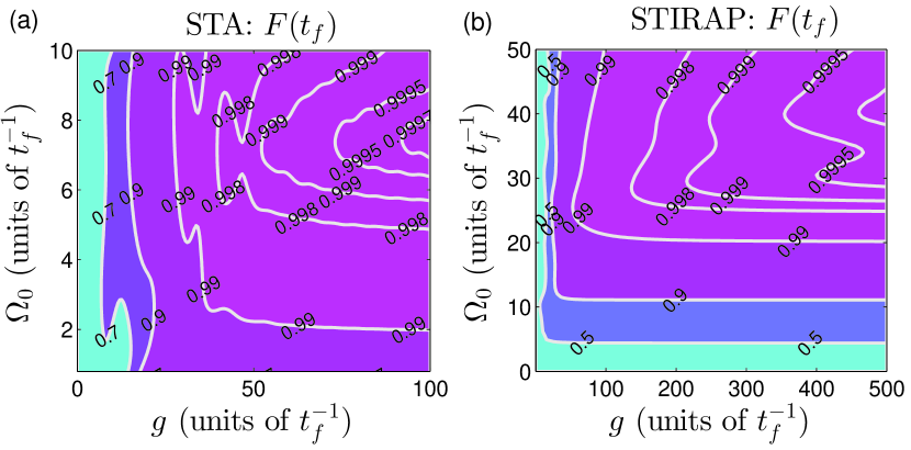
Figure 3: Contour images for final fidelities versus $g$ and $\Omega_{0}$ in (a) the STA scheme, i.e., superadiabatic scheme and (b) the STIRAP scheme.

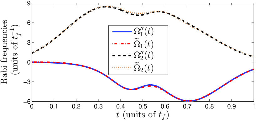
Figure 4: Time dependence of $\Omega^{\prime\prime}_{1}(t)$, $\Omega^{\prime\prime}_{2}(t)$, $\widetilde{\Omega}_{1}(t)$ and $\widetilde{\Omega}_{2}(t)$.

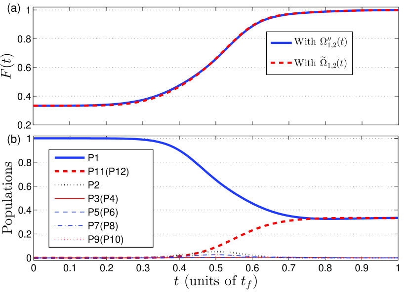
Figure 5: (a) Comparison between the fidelities for adopting {$\Omega^{\prime\prime}_{1}(t)$,$\Omega^{\prime\prime}_{2}(t)$} and {$\widetilde{\Omega}_{1}(t)$,$\widetilde{\Omega}_{2}(t)$}; (b) Time evolutions of the populations for states in equation (II), respectively, with {$\widetilde{\Omega}_{1}(t)$,$\widetilde{\Omega}_{2}(t)$}}.

Since analytic functions of $\Omega^{\prime\prime}_{1}(t)$ and $\Omega^{\prime\prime}_{2}(t)$ are too complicated, for the experimental feasibility, we seek two superpositions of Gaussian functions by curve fitting to replace them, respectively

$$\widetilde{\Omega}_{1}(t)=-\sum_{m=0}^{4}\Omega_{1m}\exp[-(t-\tau_{1m})^{2}/\chi_{1m}^{2}],\quad\widetilde{\Omega}_{2}(t)=\sum_{m=0}^{4}\Omega_{2m}\exp[-(t-\tau_{2m})^{2}/\chi_{2m}^{2}],$$ (17)

with related parameters $\{\Omega_{11}=1.4695/t_{f},\Omega_{12}=2.4114/t_{f},\Omega_{13}=1.9854/t_{f},\Omega_{14}=4.4491/t_{f},\tau_{11}=0.3733t_{f},\tau_{12}=0.4424t_{f},\tau_{13}=0.6547t_{f},\tau_{14}=0.7568t_{f},\chi_{11}=0.1494t_{f},\chi_{12}=0.0939t_{f},\chi_{13}=0.1358t_{f},\chi_{14}=0.2044t_{f}\}$ for $\widetilde{\Omega}_{1}(t)$ and $\{\Omega_{21}=6.7888/t_{f},\Omega_{22}=1.1904/t_{f},\Omega_{23}=1.649/t_{f},\Omega_{24}=5.4413/t_{f},\tau_{21}=0.2814t_{f},\tau_{22}=0.3712t_{f},\tau_{23}=0.5752t_{f},\tau_{24}=0.6588t_{f},\chi_{21}=0.2204t_{f},\chi_{22}=0.12t_{f},\chi_{23}=0.0987t_{f},\chi_{24}=0.2475t_{f}\}$ for $\widetilde{\Omega}_{2}(t)$. Through plotting figure 4, we see that the curve for $\widetilde{\Omega}_{1}(t)$ ($\widetilde{\Omega}_{2}(t)$) is very close to that for $\Omega^{\prime\prime}_{1}(t)$ ($\Omega^{\prime\prime}_{2}(t)$). In the following, for showing the effectiveness of two alternative Rabi frequencies, in figure 5(a) we plot time dependence of the fidelity for adopting $\Omega^{\prime\prime}_{1}(t)$ and $\Omega^{\prime\prime}_{2}(t)$ or $\widetilde{\Omega}_{1}(t)$ and $\widetilde{\Omega}_{2}(t)$. Highly approximate coincidences of two pairs of curves indicate that the alternative Rabi frequencies are pretty valid. For a further illustration, with $\widetilde{\Omega}_{1}(t)$ and $\widetilde{\Omega}_{2}(t)$, in figure 5(b) we plot time evolutions of the populations for all states in equation (II), respectively, and the results show that the desired two-atom 3D entanglement $|\Psi_{\rm 3D}\rangle$ can be obtained near perfectly at $t=t_{f}$. What’s more, we also see that the states not involved in $|\Psi_{\rm 3D}\rangle$ are hardly populated.

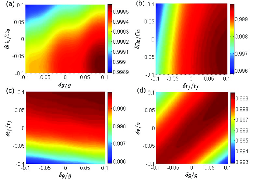
Figure 6: Effects of variations in various parameters on the final fidelity.

Since most parameters are impossible to control perfectly in experiment, we should investigate the robustness of the scheme against variations in control parameters. Here we define $\delta x=x^{\prime}-x$ as the deviation of $x$, in which $x$ denotes the ideal value and $x^{\prime}$ denotes the actual value. In figure 6, we consider effects of variations in parameters involved in the superadiabatic scheme on the final fidelity for fast generating the 3D entanglement between two atoms. As we can see from figure 6, the final fidelity always keep over $0.993$ even when variations in two of parameters we consider are both up to $|\delta x|=0.1x$, which indicates the superadiabatic scheme for fast generating the two-atom 3D entanglement is extremely robust against variations in control parameters. By the way, figure 6(d) also shows the condition $v=g$ is a little bit critical for the high-fidelity generation of the target state.

Finally, taking decoherence caused by atomic spontaneous emissions and photon leakages from the cavity-fiber system into account, the evolution of the whole system will be dominated by the master equation

$$\dot{\rho}(t) = -i[H(t),\rho(t)]$$ (18)

$$-\sum_{j=g,L,R}\frac{\gamma_{j}^{\rm A}}{2}[\sigma^{\rm A}_{e,e}\rho(t)-2\sigma^{\rm A}_{j,e}\rho(t)\sigma^{\rm A}_{e,j}+\rho(t)\sigma^{\rm A}_{e,e}]$$

$$-\sum_{j=0,L,R}\sum_{i=L,R}\frac{\gamma_{j,i}^{\rm B}}{2}[\sigma^{\rm B}_{e_{i},e_{i}}\rho(t)-2\sigma^{\rm B}_{j,e_{i}}\rho(t)\sigma^{\rm B}_{e_{i},j}+\rho(t)\sigma^{\rm B}_{e_{i},e_{i}}],$$

$$-\sum_{i=L,R}\sum_{l={\rm A,B}}\frac{\kappa_{i}^{l}}{2}[a_{li}^{{\dagger}}a_{li}\rho(t)-2a_{li}\rho(t)a_{li}^{{\dagger}}+\rho(t)a_{li}^{\dagger}a_{li}]$$

$$-\sum_{i=L,R}\frac{\kappa_{i}^{f}}{2}[b_{i}^{{\dagger}}b_{i}\rho(t)-2b_{i}\rho(t)b_{i}^{{\dagger}}+\rho(t)b_{i}^{\dagger}b_{i}],$$

where $H(t)$ is Hamiltonian (1); $\gamma_{j}^{l}$ is the photon leakage rate of atom $l$ from excited states to the ground state $|j\rangle$; $\kappa_{i}^{l}$ is the $i$-circular polarized photon leakage rate of cavity $l$; $\kappa_{i}^{f}$ is the $i$-circular polarized photon leakage rate of the fiber; $\sigma_{m,n}=|m\rangle\langle n|$. For simplicity, we assume $\gamma_{j}^{\rm A}=\gamma_{j,i}^{\rm B}=\gamma/2$, $\kappa_{i}^{l}=\kappa_{i}^{f}=\kappa$.

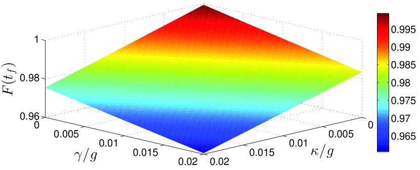
Figure 7: Final fidelity versus $\kappa/g$ and $\gamma/g$.

Based on the master equation, in figure (7) we plot the final fidelity $F(t_{f})=|\langle\Psi_{\rm 3D}|\rho(t)|\Psi_{\rm 3D}\rangle|$ for fast generating two-atom 3D entanglement versus $\kappa/g$ and $\gamma/g$. We can clearly see that the superadiabatic scheme is very robust against decoherence induced by atomic spontaneous emissions and cavity-fiber photon leakages, because even when $\kappa=\gamma=0.02g$, the final fidelity can keep very high $F(t_{f})>0.96$. For a real experiment, ${}^{87}\emph{Rb}$ and a set of predicted cavity-QED parameters $(\lambda,\kappa,\gamma)/2\pi=(750,3.5,2.62)$ MHz STO2003 ; STK2005 can be used for generating two-atom 3D entanglement in the superadiabatic scheme, and the final fidelity can reach $99.93\%$.

V Conclusion

In conclusion, we have implemented the fast generation of 3D entanglement between two atoms in an experimentally feasible superadiabatic scheme. Under the certain limit condition, the complicated system is simplified to a three-state system, which makes the superadiabatic scheme more convenient to be applied for generating two-atom 3D entanglement. Because of the compensation for non-adiabatic couplings, the adiabatic approximation is not needed. Compared with TQD, the superadiabatic scheme is more complicated just in terms of mathematical calculations. But it does not require a direct coupling between the initial and finial states, which greatly enhances experimental feasibility. In addition, the results of numerical simulations show that the superadiabatic scheme is strongly robust against variations in various parameters and decoherence caused by atomic spontaneous emissions and cavity-fiber photon leakages.

ACKNOWLEDGMENT

This work was supported by the National Natural Science Foundation of China under Grants No. 11464046.

References

(1)
Bourennane M, Karlsson A and Björk G 2001 Phys. Rev. A 64 012306
(2)
Bruß D and Macchiavello C 2002 Phys. Rev. Lett.88 127901
(3)
Cerf N J, Bourennane M, Karlsson A and Gisin N 2002 Phys. Rev. Lett.88 127902
(4)
Jo Y and Son W 2016 Phys. Rev. A 94 052316
(5)
Kaszlikowski D, Gnacinski P, Żukowski M, Miklaszewski W and Zeilinger A 2000 Phys. Rev. Lett.85 4418–4421
(6)
Shao X Q, Wang H F, Chen L, Zhang S, Zhao Y F and Yeon K H 2010 New J. Phys.12 023040
(7)
Chen L B, Shi P, Zheng C H and Gu Y J 2012 Opt. Express20 14547–14555
(8)
Liang Y, Su S L, Wu Q C, Ji X and Zhang S 2015 Opt. Express23 5064–5077
(9)
Song C, Su S L, Wu J L, Wang D Y, Ji X and Zhang S 2016 Phys. Rev. A 93 062321
(10)
Li W A and Huang G Y 2011 Phys. Rev. A 83 022322
(11)
Liu S, Li J, Yu R and Wu Y 2013 Phys. Rev. A 87 062316
(12)
Wu Q C and Ji X 2013 Quant. Inf. Process.12 3167–3178
(13)
Shao X Q, Zheng T Y, Oh C H and Zhang S 2014 Phys. Rev. A 89 012319
(14)
Su S L, Shao X Q, Wang H F and Zhang S 2014 Sci. Rep.4 07566
(15)
Wang D Y, Wen J J, Bai C H, Hu S, Cui W X, Wang H F, Zhu A D and Zhang S 2015 Annals of Physics360 228–236
(16)
Bergmann K, Theuer H and Shore B W 1998 Rev. Mod. Phys.70 1003–1025
(17)
Král P, Thanopulos I and Shapiro M 2007 Rev. Mod. Phys.79 53–77
(18)
Chen X, Ruschhaupt A, Schmidt S, del Campo A, Guéry-Odelin D and Muga J G 2010 Phys. Rev. Lett.104 063002
(19)
Chen X, Lizuain I, Ruschhaupt A, Guéry-Odelin D and Muga J G 2010 Phys. Rev. Lett.105 123003
(20)
Ibáñez S, Chen X, Torrontegui E, Muga J G and Ruschhaupt A 2012 Phys. Rev. Lett.109 100403
(21)
del Campo A, Rams M M and Zurek W H 2012 Phys. Rev. Lett.109 115703
(22)
Ruschhaupt A, Chen X, Alonso D and Muga J G 2012 New J. Phys.14 093040
(23)
Martínez-Garaot S, Torrontegui E, Chen X, Modugno M, Guéry-Odelin D, Tseng S Y and Muga J G 2013 Phys. Rev. Lett.111 213001
(24)
del Campo A 2013 Phys. Rev. Lett.111 100502
(25)
Torrontegui E, Ibáñez S, Martínez-Garaot S, Modugno M, del Campo A, Guéry-Odelin D,
Ruschhaupt A, Chen X and Muga J G 2013 Adv. At. Mol. Opt. Phys.62 117
(26)
Guéry-Odelin D, Muga J G, Ruiz-Montero M J and Trizac E 2014 Phys. Rev. Lett.112 180602
(27)
Chen Y H, Xia Y, Wu Q C, Huang B H and Song J 2016 Phys. Rev. A 93 052109
(28)
Baksic A, Ribeiro H and Clerk A A 2016 Phys. Rev. Lett.116 230503
(29)
Lu M, Xia Y, Shen L T, Song J and An N B 2014 Phys. Rev. A 89 012326; 2014 Laser Phys.24 105201
(30)
Chen Y H, Xia Y, Chen Q Q and Song J 2014 Phys. Rev. A 89 033856; 2015 Sci. Rep.5 15616; 2015 Phys. Rev. A 91 012325; 2014 Laser Phys. Lett.11 115201
(31)
Shi X and Wei L F 2015 Laser Phys. Lett.12 015204
(32)
Zhang J, Kyaw T H, Tong D M, Sjöqvist E and Kwek L C 2015 Sci. Rep.5 18414
(33)
Liang Y, Wu Q C, Su S L, Ji X and Zhang S 2015 Phys. Rev. A 91 032304; Liang Y, Song C, Ji X and Zhang S 2015 Opt. Express23 23798–23810; Liang Y, Ji X, Wang H F and Zhang S 2015 Laser Phys. Lett.12 115201
(34)
Song X K, Zhang H, Ai Q, Qiu J and Deng F G 2016 New J. Phys.18 023001
(35)
Lin J B, Liang Y, Song C, Ji X and Zhang S 2016 J. Opt. Soc. Am. B 33 519–524
(36)
Chen Z, Chen Y H, Xia Y, Song J and Huang B H 2016 Sci. Rep.6 22202
(37)
Wu J L, Song C, Ji X and Zhang S 2016 J. Opt. Soc. Am. B 33 2026–2032
(38)
He S, Su S L, Wang D Y, Sun W M, Bai C H, Zhu A D, Wang H F and Zhang S 2016 Sci. Rep.6 30929
(39)
Wu J L, Ji X and Zhang S 2016 Sci. Rep.6 33669
(40)
Berry M V 1987 Proc. R. Soc. A 414 31
(41)
Ibáñez S, Chen X and Muga J G 2013 Phys. Rev. A 87 043402
(42)
Song X K, Ai Q, Qiu J and Deng F G 2016 Phys. Rev. A 93 052324
(43)
Huang B H, Chen Y H, Wu Q C, Song J and Xia Y, Laser Phys. Lett.13 105202
(44)
Kang Y H, Chen Y H, Wu Q C, Huang B H, Song J and Xia Y 2016 Sci. Rep.6 36737
(45)
Serafini A, Mancini S and Bose S 2006 Phys. Rev. Lett.96 010503
(46)
Demirplak M and Rice S A 2003 J. Phys. Chem. A 107 9937; 2008 J. Chem. Phys.129 154111
(47)
Berry M V 2009 J. Phys. A 42 365303
(48)
Vitanov N V, Halfmann T, Shore B W and Bergmann K 2001 Annu. Rev. Phys. Chem.52 763
(49)
Spillane S M, Kippenberg T J, Painter O J and Vahala K J 2003 Phys. Rev. Lett.91 043902
(50)
Spillane S M, Kippenberg T J, Vahala K J, Goh K W, Wilcut E and Kimble H J 2005 Phys. Rev. A 71 013817