Robust and Real-time Deep Tracking Via Multi-Scale Domain Adaptation

Abstract

Visual tracking is a fundamental problem in computer vision. Recently, some deep-learning-based tracking algorithms have been achieving record-breaking performances. However, due to the high complexity of deep learning, most deep trackers suffer from low tracking speed, and thus are impractical in many real-world applications. Some new deep trackers with smaller network structure achieve high efficiency while at the cost of significant decrease on precision. In this paper, we propose to transfer the feature for image classification to the visual tracking domain via convolutional channel reductions. The channel reduction could be simply viewed as an additional convolutional layer with the specific task. It not only extracts useful information for object tracking but also significantly increases the tracking speed. To better accommodate the useful feature of the target in different scales, the adaptation filters are designed with different sizes. The yielded visual tracker is real-time and also illustrates the state-of-the-art accuracies in the experiment involving two well-adopted benchmarks with more than 100 test videos.

Index Terms—  visual tracking, deep learning, real-time

1 Introduction

Visual tracking is one of the long standing computer vision tasks. During the last decade, as the surge of deep learning, more and more tracking algorithms benefit from deep neural networks, e.g. Convolutional Neural Networks [1, 2] and Recurrent Neural Networks [3, 4]. Despite the well-admitted success, a dilemma still existing in the community is that, deep learning increases the tracking accuracy, while at the cost of high computational complexity. As a result, most well-performing deep trackers usually suffer from low efficiency [5, 6]. Recently, some real-time deep trackers were proposed [7, 8]. They achieved very fast tracking speed, but can not beat the shallow methods in some important evaluations, as we illustrate latter.

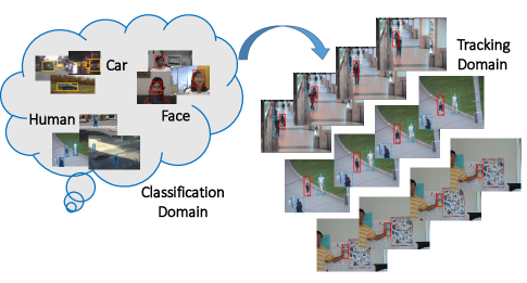
Fig. 1: The high level concept of the proposed MSDAT tracker. Left: most of the deep neural network is pretrained for image classification, where the learning algorithm focus on object classes. Right: an adaptation is performed to transfer the classification features to the visual tracking domain, where the learning algorithm treats the individual object independently.

In this paper, a simple yet effective domain adaptation algorithm is proposed. The facilitated tracking algorithm, termed Multi-Scale Domain Adaptation Tracker (MSDAT), transfers the features from the classification domain to the tracking domain, where the individual objects, rather than the image categories, play as the learning subjects. In addition, the adaptation could be also viewed as a dimension-reduction process that removes the redundant information for tracking, and more importantly, reduces the channel number significantly. This leads to a considerable improvement on tracking speed. Figure 1 illustrates the adaptation procedure. To accommodate the various features of the target object in different scales, we train filters with different sizes, as proposed in the Inception network [9] in the domain adaptation layer. Our experiment shows that the proposed MSDAT algorithm runs in around $35$ FPS while achieves very close tracking accuracy to the state-of-the-art trackers. To our best knowledge, our MSDAT is the best-performing real-time visual tracker.

2 Related work

Similar to other fields of computer vision, in recent years, more and more state-of-the-art visual trackers are built on deep learning. [1] is a well-known pioneering work that learns deep features for visual tracking. The DeepTrack method [10, 2] learns a deep model from scratch and updates it online and achieves higher accuracy. [11, 12] adopt similar learning strategies, i.e., learning the deep model offline with a large number of images while updating it online for the current video sequence. [13] achieves real-time speed via replacing the slow model update with a fast inference process.

The HCF tracker [5] extracts hierarchical convolutional features from the VGG-19 network [14], then puts the features into correlation filters to regress the respond map. It can be considered as a combination between deep learning and the fast shallow tracker based on correlation filters. It achieves high tracking accuracy while the speed is around $10$ fps. Hyeonseob Nam et al. proposed to pre-train deep CNNs in multi domains, with each domain corresponding to one training video sequence [6]. The authors claim that there exists some common properties that are desirable for target representations in all domains such as illumination changes. To extract these common features, the authors separate domain-independent information from domain-specific layers. The yielded tracker, termed MD-net, achieves excellent tracking performance while the tracking speed is only $1$ fps.

Recently, some real-time deep trackers have also been proposed. In [7], David Held et al. learn a deep regressor that can predict the location of the current object based on its appearance in the last frame. The tracker obtains a much faster tracking speed (over $100$ fps) comparing to conventional deep trackers. Similarly, in [8] a fully-convolutional siamese network is learned to match the object template in the current frame. It also achieves real-time speed. Even though these real-time deep trackers also illustrate high tracking accuracy, there is still a clear performance gap between them and the state-of-the-art deep trackers.

3 The proposed method

In this section, we introduce the details of the proposed tracking algorithm, i.e., the Multi-Scale Domain Adaptation Tracker (MSDAT).

3.1 Network structure

In HCF [5], deep features are firstly extracted from multiple layers from the VGG-19 network [14], and a set of KCF [15] trackers are carried out on those features, respectively. The final tracking prediction is obtained in a weighted voting manner. Following the setting in [5], we also extract the deep features from $conv3\_5$, $conv4\_5$ and $conv5\_5$ network layers of the VGG-19 model. However, the VGG-19 network is pre-trained using the ILSVRC dataset [16] for image classification, where the learning algorithm usually focus on the object categories. This is different from visual tracking tasks, where the individual objects are distinguished from other ones (even those from the same category) and the background. Intuitively, it is better to transfer the classification features into the visual tracking domain.

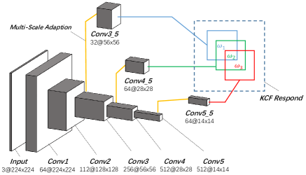
Fig. 2: The network structure of the proposed MSDAT tracker. Three layers, namely, $conv3\_5$, $conv4\_5$ and $conv5\_5$ are selected as feature source. The domain adaption (as shown in yellow lines) reduces the channel number by $8$ times and keeps feature map size unchanged. Better viewed in color.

In this work, we propose to perform the domain adaptation in a simple way. A “tracking branch” is “grafted” onto each feature layer, as shown in Fig. 2. The tracking branch is actually a convolution layer which reduces the channel number by $8$ times and keeps feature map size unchanged. The convolution layer is then learned via minimizing the loss function tailored for tracking, as introduced below.

3.2 Learning strategy

The parameters in the aforementioned tracking branch is learned following a similar manner as Single Shot MultiBox Detector (SSD), a state-of-the-art detection algorithm [17]. When training, the original layers of VGG-19 (i.e. those ones before $convx\_5$ are fixed and each “tracking branch” is trained independently) The flowchart of the learning procedure for one tracking branch (based on $conv3\_4$) is illustrated in upper row of Figure 3, comparing with the learning strategy of MD-net [6] (the bottom row). To obtain a completed training circle, the adapted feature in $conv3\_5$ is used to regress th objects’ locations and their objectness scores (shown in the dashed block). Please note that the deep learning stage in this work is purely offline and the additional part in the dashed block will be abandoned before tracking.

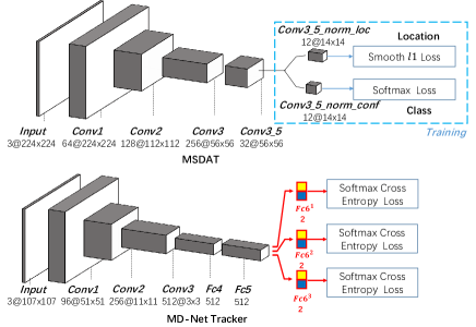
Fig. 3: The flow-charts of the training process of MSDAT and MD-net. Note that the network parts inside the dashed blocks are only used for training and will be abandoned before tracking. Better viewed in color.

In SSD, a number of “default boxes” are generated for regressing the object rectangles. Furthermore, to accommodate the objects in different scales and shapes, the default boxes also vary in size and aspect ratios. Let $m_{i,j}\in\{1,0\}$ be an indicator for matching the $i$-th default box to the $j$-th ground truth box. The loss function of SSD writes:

$$L(m,c,l,g)=\frac{1}{N}\left(L_{conf}(m,c)+\alpha L_{loc}(m,l,g)\right)$$ (1)

where $c$ is the category of the default box, $l$ is the predicted bounding-box while $g$ is the ground-truth of the object box, if applicable. For the $j$-th default box and the $i$-th ground-truth, the location loss $L^{i,j}_{loc}$ is calculated as

$$L^{i,j}_{loc}(l,g)=\sum_{u\in\{x,y,w,h\}}m_{i,j}\cdot\text{smooth}_{L_{1}}(l^{u}_{i}-\hat{g}^{u}_{j})$$ (2)

where $\hat{g}^{u},u\in\{x,y,w,h\}$ is one of the geometry parameter of normalized ground-truth box.

However, the task of visual tracking differs from detection significantly. We thus tailor the loss function for the KCF algorithm, where both the object size and the KCF window size are fixed. Recall that, the KCF window plays a similar role as default boxes in SSD [15], we then only need to generate one type of default boxes and the location loss $L^{i,j}_{loc}(l,g)$ is simplified as

$$L^{i,j}_{loc}(l,g)=\sum_{u\in\{x,y\}}m_{i,j}\cdot\text{smooth}_{L_{1}}(l^{u}_{i}-g^{u}_{j})$$ (3)

In other words, only the displacement $\{x,y\}$ is taken into consideration and there is no need for ground-truth box normalization.

Note that the concept of domain adaptation in this work is different from that defined in MD-net [6], where different video sequences are treated as different domains and thus multiple fully-connected layers are learned to handle them (see Figure 3). This is mainly because in MD-net samples the training instances in a sliding-window manner, An object labeled negative in one domain could be selected as a positive sample in another domain. Given the training video number is $C$ and the dimension of the last convolution layer is $d_{c}$, the MD-net learns $C$ independent $d_{c}\times 2$ fully-connected alternatively using $C$ soft-max losses, i.e.,

$$\mathcal{M}^{i}_{fc}:\mathbb{R}^{d_{c}}\rightarrow\mathbb{R}^{2},\forall i=1,2,\dots,C$$ (4)

where $\mathcal{M}^{i}_{fc},\forall i\in\{1,2,\dots,C\}$ denotes the $C$ fully-connected layers that transferring the common visual domain to the individual object domain, as shown in Figure 3.

Differing from the MD-net, the domain in this work refers to a general visual tracking domain, or more specifically, the KCF domain. It is designed to mimic the KCF input in visual tracking (see Figure 3). In this domain, different tracking targets are treated as one category, i.e., objects. When training, the object’s location and confidence (with respect to the objectness) are regressed to minimize the smoothed $l_{1}$ loss. Mathematically, we learn a single mapping function $\mathcal{M}_{conv}(\cdot)$ as

$$\mathcal{M}_{msdat}:\mathbb{R}^{d_{c}}\rightarrow\mathbb{R}^{4}$$ (5)

where the $\mathbb{R}^{4}$ space is composed of one $\mathbb{R}^{2}$ space for displacement $\{x,y\}$ and one label space $\mathbb{R}^{2}$.

Compared with Equation 4, the training complexity in Equation 5 decreases and the corresponding convergence becomes more stable. Our experiment proves the validity of the proposed domain adaptation.

3.3 Multi-scale domain adaptation

As introduced above, the domain adaption in our MSDAT method is essentially a convolution layer. To design the layer, an immediate question is how to select a proper size for the filters. According to Figure 2, the feature maps from different layers vary in size significantly. It is hard to find a optimal filer size for all the feature layers. Inspired by the success of Inception network [9], we propose to simultaneously learn the adaptation filters in different scales. The response maps with different filter sizes are then concatenated accordingly, as shown in Figure 4. In this way, the input of the KCF tracker involves the deep features from different scales.

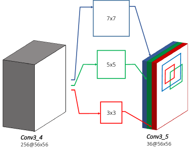
Fig. 4: Learn the adaptation layer using three different types of filters

In practice, we use $3\times 3$ and $5\times 5$ filters for all the three feature layers. Given the original channel number is $K$, each type of filter generate $\frac{K}{16}$ channels and thus the channel reduction ratio is still $8:1$.

3.4 Make the tracker real-time

3.4.1 Channel reduction

One important advantage of the proposed domain adaptation is the improvement of the tracking speed. It is easy to see that the speed of KCF tracker drops dramatically as the channel number increase. In this work, after the adaptation, the channel number is shrunk by $8$ times which accelerates the tracker by $2$ to $2.5$ times.

3.4.2 Lazy feed-forward

Another effective way to increase the tracking speed is to reduce the number of feed-forwards of the VGG-19 network. In HCF, the feed-forward process is conduct for two times at each frame, one for prediction and one for model update [5]. However, we notice that the displacement of the moving object is usually small between two frames. Consequently, if we make the input window slightly larger than the KCF window, one can reuse the feature maps in the updating stage if the new KCF window (defined by the predicted location of the object) still resides inside the input window. We thus propose a lazy feed-forward strategy, which is depicted in Figure 5.

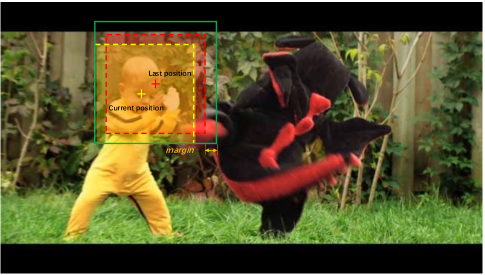
Fig. 5: The illustration of lazy feed-forward strategy. To predict the location of the object (the boy’s head), a part of the image (green window) is cropped for generating the network input. Note that the green window is slightly larger than the red block, i.e., the KCF window for predicting the current location. If the predicted location (shown in yellow) still resides inside the green lines, one can reuse the deep features by cropping the corresponding feature maps accordingly.

In this work, we generate the KCF window using the same rules as HCF tracker [5], the input window is $10\%$ larger than the KCF window, both in terms of width and height. Facilitated by the lazy feed-forward strategy, in the proposed algorithm, feed-forward is conducted only once in more than $60\%$ video frames. This gives us another $50\%$ speed gain.

4 Experiment

4.1 Experiment setting

In this section, we report the results of a series of experiment involving the proposed tracker and some state-of-the-art approaches. Our MSDAT method is compared with some well-performing shallow visual trackers including the KCF tracker [15], TGPR [18], Struck [19], MIL [20], TLD [21] and SCM [22]. Also, some recently proposed deep trackers including MD-net [6], HCF [5], GOTURN [7] and the Siamese tracker [8] are also compared. All the experiment is implemented in MATLAB with matcaffe [23] deep learning interface, on a computer equipped with a Intel i7 4770K CPU, a NVIDIA GTX1070 graphic card and 32G RAM.

The code of our algorithm is published in Bitbucket via https://bitbucket.org/xinke_wang/msdat, please refer to the repository for the implementation details.

4.2 Results on OTB-50

Similar to its prototype [24], the Object Tracking Benchmark 50 (OTB-50) [25] consists $50$ video sequences and involves $51$ tracking tasks. It is one of the most popular tracking benchmarks since the year 2013, The evaluation is based on two metrics: center location error and bounding box overlap ratio. The one-pass evaluation (OPE) is employed to compare our algorithm with the HCF [5], GOTURN [7], the Siamese tracker [8] and the afore mentioned shallow trackers. The result curves are shown in Figure 6

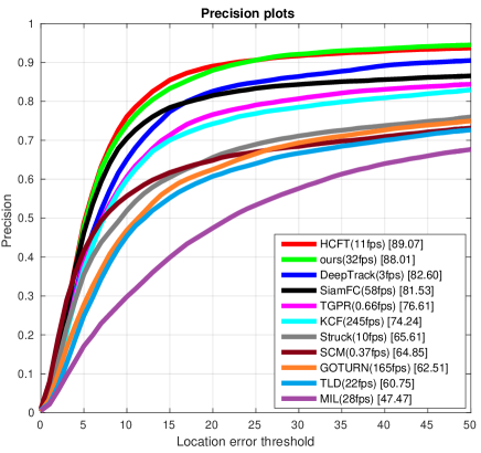
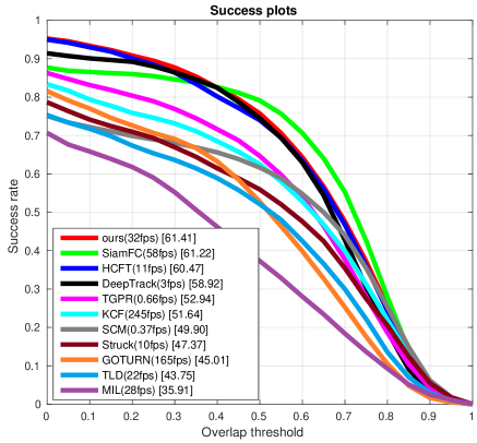
Fig. 6: The location error plots and the overlapping accuracy plots of the involving trackers, tested on the OTB-50 dataset.

From Figure 6 we can see, the proposed MSDAT method beats all the competitor in the overlapping evaluation while ranks second in the location error test, with a trivial inferiority (around $1\%$) to its prototype, the HCF tracker. Recall that the MSDAT beats the HCF with the similar superiority and runs $3$ times faster than HCF, one consider the MSDAT as a super variation of the HCF, with much higher speed and maintains its accuracy. From the perspective of real-time tracking, our method performs the best in both two evaluations. To our best knowledge, the proposed MSDAT method is the best-performing real-time tracker in this well-accepted test.

Sequence	Ours	HCF	MD-Net	SiamFC	GOTURN	KCF	Struck	MIL	SCM	TLD
DP rate(%)	83.0	83.7	90.9	75.2	56.39	69.2	63.5	43.9	57.2	59.2
OS(AUC)	0.567	0.562	0.678	0.561	0.424	0.475	0.459	0.331	0.445	0.424
Speed(FPS)	34.8	11.0	1	58	165	243	9.84	28.0	0.37	23.3

Table 1: Tracking accuracies of the compared trackers on OTB-100

4.3 Results on OTB-100

The Object Tracking Benchmark 100 is the extension of OTB-50 and contains 100 video sequences. We test our method under the same experiment protocol as OTB-50 and comparing with all the aforementioned trackers. The test results are reported in Table 1

As can be seen in the table, the proposed MSDAT algorithm keep its superiority over all the other real-time trackers and keep the similar accuracy to HCF. The best-performing MD-net (according to our best knowledge) enjoys a remarkable performance gap over all the other trackers while runs in around $1$ fps.

4.4 The validity of the domain adaptation

To better verify the proposed domain adaptation, here we run another variation of the HCF tracker. For each feature layer ($conv3\_4$, $conv4\_4$, $conv5\_4$) of VGG-19, one randomly selects one eighth of the channels from this layer. In this way, the input channel numbers to KCF are identical to the proposed MSDAT and thus the algorithm complexity of the “random HCF” and our method are nearly the same. The comparison of MSDAT, HCF and random HCF on OTB-50 is shown in Figure 7

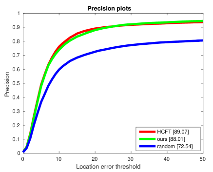
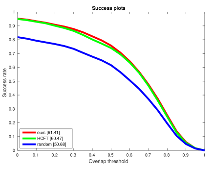
Fig. 7: The location error plots and the overlapping accuracy plots of the three version of the HCF tracker: the original HCF, the MSDAT and the random HCF method. Tested on the OTB-50 dataset, better viewed in color.

From the curves one can see a large gap between the randomized HCF and the other two methods. In other words, the proposed domain adaptation not only reduce the channel number, but also extract the useful features for the tracking task.

5 Conclusion and future work

In this work, we propose a simple yet effective algorithm to transferring the features in the classification domain to the visual tracking domain. The yielded visual tracker, termed MSDAT, is real-time and achieves the comparable tracking accuracies to the state-of-the-art deep trackers. The experiment verifies the validity of the proposed domain adaptation.

Admittedly, updating the neural network online can lift the tracking accuracy significantly [2, 6]. However, the existing online updating scheme results in dramatical speed reduction. One possible future direction could be to simultaneously update the KCF model and a certain part of the neural network (e.g. the last convolution layer). In this way, one could strike the balance between accuracy and efficiency and thus better tracker could be obtained.

References

- [1] Naiyan Wang and Dit-Yan Yeung, “Learning a deep compact image representation for visual tracking,” in NIPS, pp. 809–817. 2013.
- [2] Hanxi Li, Yi Li, and Fatih Porikli, “Deeptrack: Learning discriminative feature representations online for robust visual tracking,” IEEE Transactions on Image Processing (TIP), vol. 25, no. 4, pp. 1834–1848, 2016.
- [3] Anton Milan, Seyed Hamid Rezatofighi, Anthony Dick, Konrad Schindler, and Ian Reid, “Online multi-target tracking using recurrent neural networks,” arXiv preprint arXiv:1604.03635, 2016.
- [4] Guanghan Ning, Zhi Zhang, Chen Huang, Zhihai He, Xiaobo Ren, and Haohong Wang, “Spatially supervised recurrent convolutional neural networks for visual object tracking,” arXiv preprint arXiv:1607.05781, 2016.
- [5] Chao Ma, Jia-Bin Huang, Xiaokang Yang, and Ming-Hsuan Yang, “Hierarchical convolutional features for visual tracking,” in ICCV, 2015, pp. 3074–3082.
- [6] Hyeonseob Nam and Bohyung Han, “Learning multi-domain convolutional neural networks for visual tracking,” arXiv preprint arXiv:1510.07945, 2015.
- [7] David Held, Sebastian Thrun, and Silvio Savarese, “Learning to track at 100 fps with deep regression networks,” arXiv preprint arXiv:1604.01802, 2016.
- [8] Luca Bertinetto, Jack Valmadre, João F Henriques, Andrea Vedaldi, and Philip HS Torr, “Fully-convolutional siamese networks for object tracking,” in ECCV, 2016, pp. 850–865.
- [9] Christian Szegedy, Wei Liu, Yangqing Jia, Pierre Sermanet, Scott Reed, Dragomir Anguelov, Dumitru Erhan, Vincent Vanhoucke, and Andrew Rabinovich, “Going deeper with convolutions,” in CVPR, 2015, pp. 1–9.
- [10] Hanxi Li, Yi Li, and Fatih Porikli, “Deeptrack: Learning discriminative feature representations by convolutional neural networks for visual tracking,” BMVC, 2014.
- [11] Naiyan Wang, Siyi Li, Abhinav Gupta, and Dit-Yan Yeung, “Transferring rich feature hierarchies for robust visual tracking,” arXiv preprint arXiv:1501.04587, 2015.
- [12] Seunghoon Hong, Tackgeun You, Suha Kwak, and Bohyung Han, “Online tracking by learning discriminative saliency map with convolutional neural network,” in ICML, 2015, pp. 597–606.
- [13] Kaihua Zhang, Qingshan Liu, Yi Wu, and Ming-Hsuan Yang, “Robust tracking via convolutional networks without learning,” arXiv preprint arXiv:1501.04505, 2015.
- [14] K. Simonyan and A. Zisserman, “Very deep convolutional networks for large-scale image recognition,” CoRR, vol. abs/1409.1556, 2014.
- [15] João F Henriques, Rui Caseiro, Pedro Martins, and Jorge Batista, “High-speed tracking with kernelized correlation filters,” IEEE Transactions on Pattern Analysis and Machine Intelligence (TPAMI), vol. 37, no. 3, pp. 583–596, 2015.
- [16] Olga Russakovsky, Jia Deng, Hao Su, Jonathan Krause, Sanjeev Satheesh, Sean Ma, Zhiheng Huang, Andrej Karpathy, Aditya Khosla, Michael Bernstein, Alexander C. Berg, and Li Fei-Fei, “ImageNet Large Scale Visual Recognition Challenge,” International Journal of Computer Vision (IJCV), vol. 115, no. 3, pp. 211–252, 2015.
- [17] Wei Liu, Dragomir Anguelov, Dumitru Erhan, Christian Szegedy, and Scott Reed, “Ssd: Single shot multibox detector,” arXiv preprint arXiv:1512.02325, 2015.
- [18] Jin Gao, Haibin Ling, Weiming Hu, and Junliang Xing, “Transfer learning based visual tracking with gaussian processes regression,” in ECCV, pp. 188–203. 2014.
- [19] Sam Hare, Amir Saffari, and Philip HS Torr, “Struck: Structured output tracking with kernels,” in ICCV, 2011, pp. 263–270.
- [20] Boris Babenko, Ming-Hsuan Yang, and Serge Belongie, “Visual tracking with online multiple instance learning,” IEEE Transactions on Pattern Analysis and Machine Intelligence(TPAMI), pp. 1619–1632, 2011.
- [21] Zdenek Kalal, Jiri Matas, and Krystian Mikolajczyk, “Pn learning: Bootstrapping binary classifiers by structural constraints,” in CVPR, 2010, pp. 49–56.
- [22] Wei Zhong, Huchuan Lu, and Ming-Hsuan Yang, “Robust object tracking via sparsity-based collaborative model,” in CVPR, 2012, pp. 1838–1845.
- [23] Yangqing Jia, Evan Shelhamer, Jeff Donahue, Sergey Karayev, Jonathan Long, Ross Girshick, Sergio Guadarrama, and Trevor Darrell, “Caffe: Convolutional architecture for fast feature embedding,” in ACM MM, 2014, pp. 675–678.
- [24] Yi Wu, Jongwoo Lim, and Ming-Hsuan Yang, “Online object tracking: A benchmark,” in CVPR, 2013, pp. 2411–2418.
- [25] Yi Wu, Jongwoo Lim, and Ming-Hsuan Yang, “Object tracking benchmark,” IEEE Transactions on Pattern Analysis and Machine Intelligence (TPAMI), vol. 37, no. 9, pp. 1834–1848, 2015.