Simple bounds on fluctuations and uncertainty relations for first-passage times of counting observables

Abstract

Recent large deviation results have provided general lower bounds for the fluctuations of time-integrated currents in the steady state of stochastic systems. A corollary are so-called thermodynamic uncertainty relations connecting precision of estimation to average dissipation. Here we consider this problem but for counting observables, i.e., trajectory observables which, in contrast to currents, are non-negative and non-decreasing in time (and possibly symmetric under time reversal). In the steady state, their fluctuations to all orders are bound from below by a Conway-Maxwell-Poisson distribution dependent only on the averages of the observable and of the dynamical activity. We show how to obtain the corresponding bounds for first-passage times (times when a certain value of the counting variable is first reached) and their uncertainty relations. Just like entropy production does for currents, dynamical activity controls the bounds on fluctuations of counting observables.

I Introduction

In this note we try to connect three recent developments in the theory of stochastic systems. The first are general bounds on the fluctuations of time-integrated currents Gingrich et al. (2016); Pietzonka et al. (2016a, b); Gingrich et al. . Obtained by means “Level 2.5” Maes and Netocny (2008); Bertini et al. ; Bertini et al. (2015) dynamical large deviation methods Dembo and Zeitouni (1998); Ruelle (2004); Gaspard (2005); Lecomte et al. (2007); Touchette (2009), these results stipulate general lower bounds for fluctuations at any order of all empirical currents in the stationary state of a stochastic process Gingrich et al. (2016); Pietzonka et al. (2016a, b); Gingrich et al. . A corolary are thermodynamic uncertainty relations Barato and Seifert (2015a, b); Polettini et al. connecting the estimation error of time-integrated currents to overall dissipation.

The second development are fluctuation relations for first-passage times (FPTs) Roldán et al. (2015); Saito and Dhar (2016); Neri et al. , similar to those of more standard observables such as work or entropy production. From these an uncertainty relation connecting dissipation to the time needed to determine the direction of time can be derived Roldán et al. (2015). These results indicate a relation between the fluctuations of observables in dynamics over a fixed time, with fluctuations in stopping times.

The third development is trajectory ensemble equivalence Chetrite and Touchette (2013, 2015); Budini et al. (2014); Kiukas et al. (2015) between ensembles of long trajectories subject to different constraints. For example, for long times, the ensemble of trajectories conditioned on a fixed value of a time-integrated quantity is equivalent to that conditioned only on its average Chetrite and Touchette (2013, 2015) (cf. microcanonical/canonical equivalence of equilibrium ensembles Peliti (2011)). Similarly, the ensemble of trajectories of fixed total time and fluctuating number of jumps is equivalent to that of fixed number of jumps but fluctuating time Budini et al. (2014); Kiukas et al. (2015) (cf. fixed volume and fixed pressure static ensembles Peliti (2011)).

The works in Refs.  Gingrich et al. (2016); Pietzonka et al. (2016a, b); Gingrich et al. and Barato and Seifert (2015a, b); Polettini et al. ; Roldán et al. (2015); Saito and Dhar (2016); Neri et al. focus on trajectory observables asymmetric under time reversal, such as empirical currents, which can be positive or negative and can increase and decrease with time. Here we consider instead trajectory observables which are always non-negative and strictly non-decreasing with time. We call these counting observables. An example is the total number of configuration changes in a trajectory, or dynamical activity Lecomte et al. (2007); Garrahan et al. (2007); Maes and Netocny (2008). Here show that from the bounds to the rate functions of counting observables, via trajectory ensemble equivalence, we can derive the corresponding bounds for arbitrary fluctuations of FPTs.

After introducing the basics of dynamical large deviations, in Sec. III we show that the rate functions of counting observables are bounded from above by a Conway-Maxwell-Poisson distribution (a generalisation of the Poisson distribution that allows for non-Poissonian number fluctuations Shmueli et al. (2005)). The corresponding bound for the cumulant generating function was first found in Ref. Pietzonka et al. (2016a) (called “exponential bound”); here we rederive it straightforwardly via Level 2.5 large deviations, cf. Gingrich et al. (2016). In Sec. IV we consider the large deviations of FPTs and establish the correspondence between the FTP and observable generating functions. This allows, in Sec. V, to derive a general bound on FPT rate functions from the large deviations of the observable distributions. From these bounds FPT uncertainty relations follow. An important observation is that the bounds on fluctuations of a counting observable and its FPTs are controlled by the average dynamical activity, in analogy to the role played by the entropy production in the case of currents Gingrich et al. (2016); Barato and Seifert (2015a). We hope these results will add to the growing body of work applying large deviation ideas and methods to the study of non-equilibrium dynamics in classical and quantum stochastic systems, see e.g., Lebowitz and Spohn (1999); Evans (2004); Merolle et al. (2005); Appert-Rolland et al. (2008); Garrahan et al. (2009); Baiesi et al. (2009); Hedges et al. (2009); Kurchan ; Esposito et al. (2009); Garrahan and Lesanovsky (2010); Giardina et al. (2011); Budini (2011); Speck and Garrahan (2011); Speck et al. (2012); Bodineau and Toninelli (2012); Flindt and Garrahan (2013); Weber et al. (2013); Espigares et al. (2013); Mey et al. (2014); Vaikuntanathan et al. (2014); Weber et al. (2015); Jack et al. (2015); Ueda and Sasa (2015); De Bacco et al. ; Szavits-Nossan and Evans (2015); Jack and Sollich (2015); van Horssen and Guţă (2015); Pigeon et al. (2015); Verley (2016); Bonanca and Jarzynski (2016); Nemoto et al. (2016); Speck ; Jack and Evans ; Gherardini et al. (2016); Deffner (2016); Karevski and Schütz .

II Stochastic dynamics and large deviations of counting observables

We consider systems evolving as continuous time Markov chains Gardiner (2004), with master equation,

$$\partial_{t}P_{t}(x)=\sum_{x,y\neq x}W_{yx}P_{t}(y)-\sum_{x}R_{x}P_{t}(x),$$ (1)

where $P_{t}(x)$ is the probability being in configuration $x$ at time $t$, $W_{xy}$ the transition rate from $x$ to $y$, and $R_{x}=\sum_{y\neq x}W_{xy}$ the escape rate from $x$. In operator form the master equation reads,

$$\partial_{t}|P_{t}\rangle=\mathcal{L}|P_{t}\rangle,$$ (2)

with probability vector $|P_{t}\rangle=\sum_{x}P_{t}(x)|x\rangle$, where $\{|x\rangle\}$ is an orthonormal configuration basis. The master operator is,

$$\mathcal{L} =\mathcal{W}-\mathcal{R}=\sum_{x,y\neq x}W_{xy}|y\rangle\langle x|-\sum_{x}R_{x}|x\rangle\langle x|,$$ (3)

where $\mathcal{W}$ and $\mathcal{R}$ indicate the off-diagonal and diagonal parts of $\mathcal{L}$, respectively. This dynamics is realised by stochastic trajectories, such as $\omega=(x_{0}\to x_{t_{1}}\to\ldots\to x_{t_{K}})$. This trajectory has $K$ jumps, with the jump between configurations $x_{t_{i-1}}$ and $x_{t_{i}}$ occurring at time $t_{i}$, with $0\leq t_{1}\leq\cdots t_{K}\leq t$, and no jump between $t_{K}$ and $t$. We denote by $\pi_{t}(\omega)$ the probability of $\omega$ within the ensemble of trajectories of total time $t$.

Properties of the dynamics are encoded in trajectory observables, i.e., functions of the whole trajectory, $\mathbb{A}(\omega)$, which are extensive in time. Examples include time-integrated currents or dynamical activities. Time-exentisivity implies that at long times their probabilities and moment generating functions have large deviation forms Dembo and Zeitouni (1998); Ruelle (2004); Gaspard (2005); Lecomte et al. (2007); Touchette (2009),

$$P_{t}(A) =\sum_{\omega}\delta\left[A-\mathbb{A}(\omega)\right]\pi_{t}(\omega)\approx e^{-t\varphi(A/t)},$$ (4)

$$Z_{t}(s) =\sum_{\omega}e^{-s\mathbb{A}(\omega)}\pi_{t}(\omega)\approx e^{t\theta(s)},$$ (5)

where the rate function $\varphi(a)$ and the scaled cumulant generating function $\theta(s)$ are related by a Legendre transform Dembo and Zeitouni (1998); Ruelle (2004); Gaspard (2005); Lecomte et al. (2007); Touchette (2009),

$$\varphi(a)=-\min_{s}\left[\theta(s)+s\,a\right].$$ (6)

In what follows we focus on trajectory observables defined in terms of the jumps in a trajectory,

$$\mathbb{A}(\omega)=\sum_{xy}\alpha_{xy}\mathbb{Q}_{xy}(\omega),$$ (7)

where $\mathbb{Q}_{xy}(\omega)$ is the number of jumps from $x$ to $y$ in trajectory $\omega$. We will assume all $\alpha_{xy}\geq 0$. This means that $\mathbb{A}(\omega)$ is non-negative and non-decreasing with time. We call $\mathbb{A}(\omega)$ a counting observable as it counts the number of certain kinds of jumps in the trajectory. Furthermore, when $\alpha_{xy}=\alpha_{yx}$ these observables are symmetric under time-reversal, in contrast to time-integrated currents which are antisymmetric (and therefore neither necessarily positive nor non-decreasing with time). An important example of a counting observable is the total number of jumps or dynamical activity Lecomte et al. (2007); Garrahan et al. (2007); Maes and Netocny (2008),

$$\mathbb{K}(\omega)=\sum_{xy}\mathbb{Q}_{xy}(\omega).$$ (8)

For observables such as Eq. (7) the moment generating function Eq. (5) can be written as

$$Z_{t}(s)=\langle-|e^{t\mathcal{L}_{s}}|x_{0}\rangle,$$ (9)

where $\mathcal{L}_{s}$ is the tilted operator Dembo and Zeitouni (1998); Ruelle (2004); Gaspard (2005); Lecomte et al. (2007); Touchette (2009),

$$\mathcal{L}_{s}=\mathcal{W}_{s}-\mathcal{R}=\sum_{x,y\neq x}e^{-\alpha_{xy}s}W_{xy}|y\rangle\langle x|-\mathcal{R},$$ (10)

and $\langle-|=\sum_{x}\langle x|$. The function $\theta(s)$ is then given by the largest eigenvalue of $\mathcal{L}_{s}$.

III Level 2.5 and fluctuation bounds

The computation of large deviation functions as the ones in Eqs. (4) and (5) for arbitrary observables and dynamics is difficult in general. There is however one case where the rate function can be written down explicitly Maes and Netocny (2008); Bertini et al. ; Bertini et al. (2015).

If we denote by $\mathbb{M}_{x}(\omega)$ the total residence time in configuration $x$ throughout trajectory $\omega$, then $t^{-1}\mathbb{M}_{x}(\omega)$ is the empirical measure. Similarly, from the number of jumps $\mathbb{Q}_{xy}(\omega)$ we can define the empirical flux, $t^{-1}\mathbb{Q}_{xy}(\omega)$. Since $\mathbb{M}(\omega)$ and $\mathbb{Q}(\omega)$ are extensive observables, their probability obeys a large deviation principle at long times Dembo and Zeitouni (1998); Ruelle (2004); Gaspard (2005); Lecomte et al. (2007); Touchette (2009),

$$P_{t}(q,m)= \sum_{\omega}\pi_{t}(\omega)\prod_{x}\delta\left[m_{x}-t^{-1}\mathbb{M}_{x}(\omega)\right]$$ (11)

$$~{}~{}\times\prod_{xy}\delta\left[q_{xy}-t^{-1}\mathbb{Q}_{xy}(\omega)\right]\approx e^{-tI(q,m)}.$$

The rate function $I(q,m)$ has an explicit form in the stationary state dynamics of Eq. (2), known as “level 2.5” of large deviations Maes and Netocny (2008); Bertini et al. ; Bertini et al. (2015),

$$I(q,m)=\sum_{xy}q_{xy}\left[\ln\left(\frac{q_{xy}}{m_{x}W_{xy}}\right)-1\right]+\sum_{x}m_{x}R_{x},$$ (12)

where $m$ and $q$ must obey the probability conserving conditions,

$$\sum_{x}m_{x}=1\;,\;\;\;\sum_{y}q_{xy}=\sum_{y}q_{yx}.$$ (13)

This rate function is minimised (its minimum value being zero) when $m$ and $q$ take the stationary average values

$$m_{x}=\rho_{x}\;,\;\;q_{xy}=\rho_{x}W_{xy},$$ (14)

where $\rho_{x}$ is the stationary distribution, $\mathcal{L}|\rho\rangle=0$. The rate function for a trajectory observable such as Eq. (7) can then be obtained by contraction Dembo and Zeitouni (1998); Ruelle (2004); Gaspard (2005); Lecomte et al. (2007); Touchette (2009),

$$\varphi(a)=\min_{q,m~{}:~{}a=\alpha\cdot q}I(q,m),$$ (15)

where $\alpha\cdot q=\sum_{xy}\alpha_{xy}q_{xy}$ and $a=A/t$.

An upper bound for $\varphi(a)$ can be obtained following the procedure of Ref. Gingrich et al. (2016). From Eq. (15), any pair of empirical measure $m$ and flux $q$ that satisfies Eq. (13) and has $a=\sum_{xy}\alpha_{xy}q_{xy}$ will give an upper bound to $\varphi(a)$. A convenient and simple choice is,

$$m^{*}_{x}=\rho_{x}\;,\;\;q^{*}_{xy}=\frac{a}{\langle a\rangle}\rho_{x}W_{xy},$$ (16)

where $\langle a\rangle=\sum_{xy}\alpha_{xy}\rho_{x}W_{xy}$. We then get, with $I_{*}(a)=I(q^{*},m^{*})$,

$$\varphi(a)\leq I_{*}(a)=\frac{\langle k\rangle}{\langle a\rangle}\left[\ln\left(\frac{a}{\langle a\rangle}\right)-\left(a-\langle a\rangle\right)\right],$$ (17)

where $\langle k\rangle=\sum_{xy}\rho_{x}W_{xy}=\sum_{x}\rho_{x}R_{x}$ is the average dynamical activity (per unit time). The rate function on the right side of Eq. (17) is that of a Conway-Maxwell-Poisson (CMP) distribution Shmueli et al. (2005), a generalisation of the Poisson distribution for a counting variable with non-Poissonian number fluctuations.

From the Legendre transform Eq. (6), the upper bound Eq. (17) also implies a lower bound for the scaled cumulant generating function $\theta(s)$,

$$\theta(s)\geq\theta_{*}(s)=\langle k\rangle\left[\exp\left(-s\frac{\langle a\rangle}{\langle k\rangle}\right)-1\right].$$ (18)

The expression on the right is the scaled cumulant generating function of a CMP distribution. This last result was first derived in Ref. Pietzonka et al. (2016a) in a slightly different manner.

Figure 1 illustrates the bounds Eqs. (17) and (18) for the elementary example of a two-level system. The exact rate function $\varphi(a)$ and the upper bound $I_{*}(a)$ have the same minimum at $\langle a\rangle$, but the fluctuations of $a$ are larger than those given by $I_{*}(a)$ for all $a$. The exact cumulant generating function $\theta(s)$ and its lower bound $\theta_{*}(s)$ have the same slope at $s=0$, but $\theta_{*}(s)$ has derivatives which are smaller in magnitude to all orders that those of $\theta(s)$, again indicating that the CMP approximation provides lower bounds for the size of fluctuations of $a$.

As occurs with the analogous bounds on time-integrated currents Gingrich et al. (2016); Pietzonka et al. (2016a, b); Gingrich et al. , an immediate consequence of the bounds on the rate function or cumulant generating function are the thermodynamic uncertainty relations Barato and Seifert (2015a, b); Polettini et al. . From Eq. (17) or Eq. (18) we get a lower bound for the variance of the observable in terms of its average and the average activity (cf. Pietzonka et al. (2016a))

$${\rm var}(a)=\frac{\theta^{\prime\prime}(0)}{t}\geq\frac{\theta_{*}^{\prime\prime}(0)}{t}=\frac{\langle a\rangle^{2}}{\langle k\rangle\,t}.$$ (19)

This in turn provides an upper bound for precision of estimation of the observable $A$ in terms of the signal-to-noise ratio (i.e. inverse of the error),

$${\rm SNR}(A)=\frac{\langle A\rangle}{\sqrt{{\rm var}(A)}}\leq\sqrt{{\langle K\rangle}}\,,$$ (20)

where ${\langle K\rangle}=t{\langle k\rangle}$. Just like in the case of integrated currents Barato and Seifert (2015a, b); Polettini et al. , where there is an unavoidable tradeoff between precision and dissipation, the uncertainty in the estimation of a counting observable is bounded generically by the overall average activity in the process.

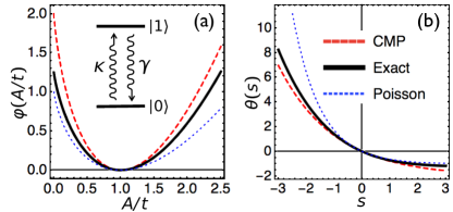
Figure 1: Bounds on observable fluctuations for a 2-level system. Transition rates are $W_{10}=\gamma$ and $W_{01}=\kappa$. We consider as observable $A$ the total number of $1\to 0$ jumps. In the stationary state $\langle a\rangle=\langle A\rangle/t=\gamma\kappa/(\gamma+\kappa)$. The average activity per unit time is $\langle k\rangle=2\langle a\rangle$. Panel (a) shows the rate function $\varphi(A/t)$ (full/black) for $\gamma=5$ and $\kappa=1.25$. The rate function is bounded from above everywhere by a CMP rate function, Eq. (17) (dashed/red). We also show for comparison a Poisson rate function with mean $\langle a\rangle$ (dotted/blue). Panel (b) shows the corresponding scaled cumulant generating function $\theta(s)=\frac{1}{2}\left[\sqrt{(\gamma-\kappa)^{2}+4\gamma\kappa e^{-s}}-(\gamma+\kappa)\right]$ (full/black). It is monotonic in $s$ since $A\geq 0$, and is bounded from below, Eq. (18), by $\theta_{*}(s)=\frac{2\gamma\kappa}{\gamma+\kappa}(e^{-s/2}-1)$ (dashed/red). For the case $\kappa=\gamma$ the bounds become exact in this simple model.

IV Large deviations of first-passage time distributions

We consider now the statistics of first-passage times (FPT) (also called stopping times), the times at which a certain trajectory observable first reaches a threshold value. This implies a change of focus from ensembles of trajectories of total fixed time to ensembles of trajectories of fluctuating overall time Bolhuis (2008); Budini et al. (2014); Harris and Touchette . Recently, distributions of FPT associated with entropy production have been shown to obey fluctuation relations Roldán et al. (2015); Saito and Dhar (2016); Neri et al. reminiscent of those of current-like observables. This suggests a duality between observable and FPT statistics, which in turn is connected to the equivalence between fixed time and fluctuating time trajectory ensembles, see e.g. Budini et al. (2014); Kiukas et al. (2015).

We focus on stopping times for counting observables as defined in Eq. (7). For simplicity we assume that the coefficients $\alpha_{xy}$ are either 0 or 1, so that $\mathbb{A}(\omega)$ counts a subset of all possible jumps in a trajectory and takes integer values. (These assumptions can be relaxed at the expense of slightly more involved expressions without changing the essence of the results.)

Lets consider the structure of trajectories associated with FPT events for a fixed value $A$ of the observable $\mathbb{A}(\omega)$. Such a trajectory will have $A$ jumps for which $\alpha_{xy}=1$, occurring at times $0\leq t_{1}\leq\cdots t_{A-1}\leq t_{A}=\tau$ with $\tau$ being the FPT through $\mathbb{A}(\omega)=A$. In between these jumps the evolution will be one where only jumps with $\alpha_{xy}=0$ occur. The weight of this trajectory is related to the amplitude of a matrix product state Garrahan (2016),

$$\langle y|\,\tilde{\mathcal{W}}\,e^{(t_{A}-t_{A-1})\mathcal{L}_{\infty}}\,\cdots\tilde{\mathcal{W}}\,e^{(t_{2}-t_{1})\mathcal{L}_{\infty}}\,\tilde{\mathcal{W}}\,e^{t_{1}\mathcal{L}_{\infty}}\,|x\rangle.$$ (21)

This expression is the weight of all trajectories starting in $x$ and ending in $y$, after $A$ jumps that contribute to the observable, occurring at the specified times $t_{i}$ ($i=1,\ldots,A$), and with an arbitrary number of the other jumps. Here $\mathcal{L}_{\infty}$ is the tilted operator Eq. (10) at $s\to\infty$, so that all transitions associated to $\mathbb{A}(\omega)$ are suppressed. The factors $e^{\Delta t\mathcal{L}_{\infty}}$ encode dynamics which do not contribute to increasing the observable and which occur between the times $t_{i}$. The operator

$$\tilde{\mathcal{W}}=\mathcal{L}-\mathcal{L}_{\infty},$$ (22)

includes all the transitions that increase $\mathbb{A}(\omega)$ by one unit, and Eq. (21) has $A$ insertions of $\tilde{\mathcal{W}}$. Integrating Eq. (21) over intermediate times and summing over the final configuration formally yields the FPT distribution,

$$F_{x}(\tau|A)=\int_{0\leq t_{1}\cdots\leq\tau}\langle-|\,\tilde{\mathcal{W}}\,e^{(\tau-t_{A-1})\mathcal{L}_{\infty}}\,\cdots\tilde{\mathcal{W}}\,e^{t_{1}\mathcal{L}_{\infty}}\,|x\rangle.$$

This expression simplifies via a Laplace transform,

$$\hat{F}_{x}(\mu|A)=\int_{0}^{\infty}dt\,e^{-\mu\tau}\,F_{x}(\tau|A)=\langle-|\mathcal{F}_{\mu}^{A}|x\rangle,$$ (23)

where the transfer operator reads

$$\mathcal{F}_{\mu}=\tilde{\mathcal{W}}\,\left(\mu-\mathcal{L}_{\infty}\right)^{-1}.$$ (24)

When $A$ is large, $A\gg 1$, the Laplace transformed FTP distribution has a large deviation form,

$$\hat{F}_{x}(\mu|A)\approx e^{Ag(\mu)},$$ (25)

where $e^{g(\mu)}$ is the largest eigenvalue of $\mathcal{F}_{\mu}$. Note the similarities between Eqs. (23-25) and Eqs. (5-10).

The eigenvalues of $\mathcal{F}_{\mu}$ and $\mathcal{L}_{s}$ are directly related. From Eqs. (10), (22) and (24) we can write,

$$e^{-s}\mathcal{F}_{\mu}=\left(\mathcal{L}_{s}-\mu\right)\left(\mu-\mathcal{L}_{\infty}\right)^{-1}+1.$$ (26)

Consider now a row vector $\langle l|$ which is a left eigenvector both of $\mathcal{F}_{\mu}$ and $\mathcal{L}_{s}$, with eigenvalue $e^{g(\mu)}$ and $\theta(s)$, respectively. Multiplying Eq. (26) by $\langle l|$ and rearranging we get

$$\left(e^{-s+g(\mu)}-1\right)\langle l|=\left[\theta(s)-\mu\right]\langle l|\left(\mu-\mathcal{L}_{\infty}\right)^{-1}.$$ (27)

We see that for $\langle l|$ to be a simultaneous eigenvector of $\mathcal{F}_{\mu}$ and $\mathcal{L}_{s}$ we need to have $g(\mu)=s$ and $\theta(s)=\mu$. That is, $g$ is the functional inverse of $\theta$ and vice-versa,

$$\theta(s)=g^{-1}(s),\;\;\;g(\mu)=\theta^{-1}(\mu).$$ (28)

For the case where the counting observable is the dynamical activity, Eq. (8), the analysis above is that of “$x$-ensemble” of Ref. Budini et al. (2014), i.e., the ensemble of trajectories of fixed total number of jumps but fluctuating time.

For the general problem of the FPTs for arbitrary counting observables, Eqs. (23-24) coincide with the FPT distributions first obtained in Ref. Saito and Dhar (2016) in a different way. The derivation in Ref. Saito and Dhar (2016) proceeds in the standard manner used for example in the proof of FPT distributions for diffusion processes Gardiner (2004). It relates the probability of having accumulated $A$ up to time $t$, to the probability of reaching $A$ at time $\tau\leq t$ for the first time followed by no increment in $A$ from $\tau$ to $t$,

$$P_{t}(A|x)=\sum_{y}\int_{0}^{t}d\tau P_{t-\tau}(0|y)F_{xy}(\tau|A),$$ (29)

where $P_{t}(A|x)$ is Eq. (4) with the initial condition made explicit, and $F_{xy}(\tau|A)$ refers to the FPT distribution for time $\tau$ and final configuration $y$. If we transform from $A$ to $s$, cf. Eqs. (4), (5) and (9), we can rewrite Eq. (29) as matrix elements of

$$e^{t\mathcal{L}_{s}}=\int_{0}^{t}d\tau e^{(t-\tau)\mathcal{L}_{\infty}}\hat{\mathcal{F}}_{s}(\tau),$$ (30)

where $\langle y|\hat{\mathcal{F}}_{s}(\tau)|x\rangle=\sum_{A}e^{-sA}F_{xy}(\tau|A)$. After a Laplace transform and rearraging we get,

$$\hat{\mathcal{F}}_{s\mu}=\left(\mu-\mathcal{L}_{\infty}\right)\left(\mu-\mathcal{L}_{s}\right)^{-1}.$$ (31)

This last expression is the same as that in Ref. Saito and Dhar (2016) after a discrete Laplace transform from $A$ to $s$. We can invert the $A\to s$ transformation as follows. The l.h.s. of Eq. (31) is,

$$\hat{\mathcal{F}}_{s\mu}=\sum_{A=0}^{\infty}e^{-sA}\hat{\mathcal{F}}_{\mu}(A),$$ (32)

while the r.h.s. can be rewritten as,

$$\left(\mu-\mathcal{L}_{\infty}\right) \left(\mu-\mathcal{L}_{s}\right)^{-1}$$

$$=\left[1-e^{-s}\tilde{\mathcal{W}}\left(\mu-\mathcal{L}_{\infty}\right)^{-1}\right]^{-1}$$

$$=\sum_{A=0}^{\infty}e^{-sA}\left[\tilde{\mathcal{W}}\left(\mu-\mathcal{L}_{\infty}\right)^{-1}\right]^{A}.$$ (33)

Equating Eqs. (32) and (33) term by term we get that

$$\hat{\mathcal{F}}_{\mu}(A)=\mathcal{F}_{\mu}^{A},$$ (34)

with $\mathcal{F}_{\mu}$ given by Eq. (24), showing that our derivation is equivalent to that of Ref. Saito and Dhar (2016). The advantage of expressing the FPT distribution in terms of its generating function Eq. (24) as we have done here is that it allows for a direct extraction of its large deviation function, see Eqs. (25) and (28), giving access to the full statistics of FPTs in the limit of large $A$.

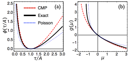
Figure 2: Bounds on first-passage time fluctuations for the 2-level system of Fig. 1. The FPT $\tau$ is defined as the time when a total $A$ of up/down jumps $1\to 0$ is reached. In the stationary state $\langle\tau\rangle=A/\langle a\rangle=A(\gamma+\kappa)/(\gamma\kappa)$. Panel (a) shows the rate function $\phi(\tau/A)$ (full/black) for $\gamma=5$ and $\kappa=1.25$, and assuming the initial state is $0$. The rate function is bounded from above everywhere by $\phi_{*}(\tau/A)$, Eq. (37) (dashed/red). We also show for comparison the FPT rate function of a Poisson process with the same mean (dotted/blue). Panel (b) shows the FPT scaled cumulant generating function $g(\mu)=\ln(\gamma\kappa)-\ln[(\gamma+\mu)(\kappa+\mu)]$ (full/black). It is bounded from below, Eq. (35), by $g_{*}(\mu)$ (dashed/red).

V Bounds on FPT distributions

Equations (23-28) establish a connection between the statistics of a counting observable, at fixed overall time, and the statistics of the FPT for a fixed value of said observable. This connection is due to the equivalence Budini et al. (2014); Kiukas et al. (2015) between the ensemble of trajectories of fixed time, but where the observable is allowed to fluctuate (in a manner controlled by the field $s$ conjugate to the observable), with the ensemble of fixed observable but where the time extension of trajectories is allowed to fluctuate (in a manner controlled by the field $\mu$ conjugate to time). This equivalence holds in the limit of large observable/time, where the relation between the controlling fields is given by Eq. (28). We can now use the results of Sec. III on bounds on observable fluctuations to infer the corresponding bounds on FPT fluctuations.

The bound Eq. (18) on the cumulant generating function of $A$ provides an lower bound to the FPT scaled cumulant generating function $g(\mu)$ through Eq. (28). Inverting $\theta_{*}$ in Eq. (18) we get

$$g(\mu)\geq g_{*}(\mu)=-\frac{\langle k\rangle}{\langle a\rangle}\ln\left(\frac{\mu}{\langle k\rangle}+1\right).$$ (35)

For large $A$ the FPT distribution also has a large deviation form,

$$F(\tau|A)\approx e^{-A\phi(\tau/A)},$$ (36)

where $\phi(\tau/A)$ is obtained from $g(\mu)$ by a Legendre transform similar to Eq. (6). From Eq. (35) we then obtain an upper bound for the FPT rate function,

$$\phi(\tau/A)\leq ~{}\phi_{*}(\tau/A)=$$ (37)

$$~{}~{}-\frac{\langle k\rangle}{\langle a\rangle}\left[\ln\left(\frac{\tau\langle a\rangle}{A}\right)-\left(\frac{\tau\langle a\rangle}{A}-1\right)\right].$$

Figure 2 illustrates the upper bound of the FPT rate function, Eq. (37), and the lower bound of the FPT cumulant generating function, Eq. (35), for the same 2-level model of Fig. 1.

The bound function $\phi_{*}(\tau/A)$ has its minimum at the exact value of the average FPT,

$$\langle\tau\rangle_{A}=\frac{A}{\langle a\rangle},$$ (38)

where $\langle\cdot\rangle_{A}$ indicates average in the FPT ensemble of fixed $A$. That the average FPT is given by the inverse of the observable per unit time follows immediately from Eq. (28). The second derivative of $\phi_{*}(\tau/A)$ at its minimum provides a lower bound for the variance of the FPT. From Eq. (37), or alternatively Eq. (35), we get,

$$\frac{{\rm var}(\tau)}{A}=g^{\prime\prime}(0)\geq g_{*}^{\prime\prime}(0)=\frac{1}{\langle a\rangle\langle k\rangle}.$$ (39)

This in turn gives a bound on the precision with which one can estimate the FPT,

$${\rm SNR}(\tau)=\frac{\langle\tau\rangle_{A}}{\sqrt{{\rm var}(\tau)}}\leq\sqrt{{\langle K_{A}\rangle}}\,.$$ (40)

where ${\langle K_{A}\rangle}=\langle\tau\rangle_{A}\langle k\rangle$. As for case of the uncertainty for the observable, Eq. (20), the precision of estimation of the FPT is limited by the total average activity, in this case for trajectories of length $t=\langle\tau\rangle_{A}$.

VI Conclusions

We have discussed general bounds on fluctuations of counting observables, hopefully complementing the more detailed recent results on current fluctuations Gingrich et al. (2016); Pietzonka et al. (2016a, b); Gingrich et al. . While empirical currents are the natural trajectory observables to consider in driven problems Gingrich et al. (2016); Pietzonka et al. (2016a, b); Gingrich et al. ; Maes and Netocny (2008); Lebowitz and Spohn (1999); Evans (2004); Appert-Rolland et al. (2008); Espigares et al. (2013); Jack et al. (2015); Karevski and Schütz , counting observables such as the dynamical activity are central quantities for systems with complex equilibrium dynamics, such as glass formers Merolle et al. (2005); Garrahan et al. (2007, 2009); Hedges et al. (2009); Speck et al. (2012). (And even for driven systems it is revealing to study the dynamical phase behaviour in terms of both empirical currents and activities, see e.g. Appert-Rolland et al. (2008); Speck and Garrahan (2011); Jack et al. (2015); Karevski and Schütz .)

The bounds are a straightforward consequence of the Level 2.5 large deviation Maes and Netocny (2008); Bertini et al. ; Bertini et al. (2015) description, Eq. (12), which provides an explicit (and useful) minimisation principle for rate functions. But as remarked in Gingrich et al. , these bounds may be more or less descriptive depending on whether they are tight or loose, which in turn depends on how good the variational ansatz is. As observed in Pietzonka et al. (2016a), the ansatz Eq. (16) is akin to a mean-field approximation that homogenises the connections between states. For any counting observable which is a subset of the overall activity the rate function is bound by a CMP distribution with sub-Poissonian number fluctuations, see Eqs. (17) and (18). For the elementary example of Fig. 1 the bound is tight, but more complex problems of interest often display large (that is, super-Poissonian) number fluctuations Merolle et al. (2005); Garrahan et al. (2007); Hedges et al. (2009); Garrahan and Lesanovsky (2010); Speck et al. (2012); Weber et al. (2013). It would be interesting to find alternative yet simple variational ansatzes that can capture such strong fluctuation behaviour. Nevertheless, there are still important consequences that follow even from these simple bounds. An immediate one is that the dynamical activity cannot be sub-Poissonian, which in turn implies an exponential in time complexity for the efficient sampling of trajectories conditioned on it, cf. Jack et al. (2015).

We have also shown how to obtain related general bounds on the distributions of first-passage times. Again this complements for counting observables, and generalises, recent results on FPTs for current-like quantities Roldán et al. (2015); Saito and Dhar (2016); Neri et al. . We did this by exploiting the correspondence between the large deviation functions of observables and those of FPTs, Eqs. (25-28). Note that this correspondence works for observables which are non-decreasing in time. For these, the zero increment probability $P_{t}(0|y)$, Eq. (29), is directly related to the tilted operator $\mathcal{L}_{\infty}$, leading to the ensemble correspondence, Eqs. (25-28). For currents, however, a zero observable does not imply the absence of jumps that contribute to the observable (only that their contribution adds up to zero), and the correspondence breaks down (or at least we have not been able to relate the corresponding cumulant generating functions in that case). Just like in the case of activities, the FPTs are bounded by the distribution of times of a CMP process, Eqs. (35) and (37), as illustrated in Fig. 2.

As occurs for currents Barato and Seifert (2015a, b); Polettini et al. , the bounds to rate functions give rise to thermodynamic uncertainty relations constraining the precision of estimation of both observables and FPTs, Eqs. (20) and (40). For empirical currents, which are time-asymmetric, precision is limited by the average entropy produced Barato and Seifert (2015a, b); Polettini et al. . In turn, for counting observables and their FPTs, the corresponding limit is set by the average dynamical activity, suggesting that this quantity might play as important a role in the dynamics as the overall dissipation.