Spatial structure of shock formation

Abstract

The formation of a singularity in a compressible gas, as described by the Euler equation, is characterized by the steepening, and eventual overturning of a wave. Using a self-similar description in two space dimensions, we show that the spatial structure of this process, which starts at a point, is equivalent to the formation of a caustic, i.e. to a cusp catastrophe. The lines along which the profile has infinite slope correspond to the caustic lines, from which we construct the position of the shock. By solving the similarity equation, we obtain a complete local description of wave steepening and of the spreading of the shock from a point.

1 Introduction

From well into the 19th century, it has been known that the equations of compressible gas dynamics form shocks, i.e. lines or surfaces across which variables change in a discontinuous fashion ([12, 23]). This makes them perhaps the earliest example of a singularity of solutions to a partial differential equation ([16]). For smooth initial data, shock formation is associated with a gradual steepening, and eventual overturning of the velocity and density profiles. A shock develops at the point where the slope first becomes infinite. The shock location can be calculated from the overturned profile via the so-called Rankine-Hugoniot conditions ([12]). The generic solution of hyperbolic (not linearly degenerate) systems in one space dimension with smooth initial data develops a cusp catastrophe, while solution to elliptic systems in one space dimension develop an elliptic umbilic catastrophe ([14]).

Relatively little emphasis has been placed on the description of how a shock is formed initially, starting from smooth initial data. The expectation is that the solution near the singular point is self-similar ([16]), but self-similar properties, in particular in more than one dimension, have also not received much attention until recently ([30, 15, 26, 27]). In the transversal direction, the size of the shock solution scales like the square root of time, a fact which is confirmed readily from observation, see Fig. 1.

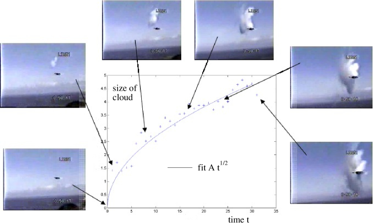
Figure 1: The spreading of a shock wave behind a supersonic plane, as marked by the condensation cloud produced by the shock. The data are based on measurements from a video (https://www.youtube.com/watch?v=gWGLAAYdbbc), with some sample images shown. Image and data analysis by Patrice Legal, used with permission. The width of the cloud scales like $t^{1/2}$, as measured from the initiation of the cloud. Absolute units of space and time are unknown.

It has been conjectured for a long time ([35, 32]) that the formation of a shock in gas dynamics is analogous to the formation of caustics of wave fields ([28]), and thus are part of the same hierarchy of singularities which can be classified using catastrophe theory ([4, 2, 3]). The simplest such singularity is the fold, which originates from a point of higher symmetry called the cusp catastrophe ([28]). Thus the cusp catastrophe is the point where the singularity is expected to occur for the first time, unless initial conditions are chosen such that the catastrophe is of higher order ([28]). Examples of experimental observations of cusp catastrophes are found in optics ([28]), shock waves ([34]), and clouds of cold atoms ([33]). Note however that the cusp catastrophe considered for example in ([34, 13, 8, 9]) appears in the shape of the shock front itself, whereas we consider the evolution of the velocity and density fields as a shock is formed.

In order to use catastrophe theory, one needs to describe the phenomenon by means of a smooth mapping, whose singularities can be classified. In optics, Fermat’s principle guarantees the existence of such a function ([28]). In the case of shock dynamics, the method of characteristics can provide an analogous function ([2]), but its existence is usually guaranteed only in one space dimension ([12]) or for the simplest purely kinematic equation ([30]). In [19] we proposed an extension of the method of characteristics for the dKP equation ([19]), which removes the singularity in the neighborhood of a shock, so that the unfolded profile can be expanded about the shock position. However, in the case of the full two or three-dimensional equations of compressible gas dynamics, no such smooth unfolding is known to exist, so catastrophe theory or an analogous method of expansion cannot be applied.

Instead, we resort to solving the equations of motion directly near the singularity, whose structure is expected to resemble the cusp catastrophe of geometrical optics. The key idea is to use the self-similar properties of the cusp catastrophe, in order to obtain a leading-order solution of the equations of motion in powers of the time distance $t^{\prime}=t_{0}-t$ to the singularity, where $t_{0}$ is the time of blow-up.

2 Equations of motion

We consider the compressible Euler equation in two space dimensions, and denote the spatial variables by $\boldsymbol{x}=(x,y)\in\mathbb{R}^{2}$. The velocity field ${\bf v}=(u,v)$ is assumed irrotational: ${\bf v}=\nabla\phi$. Before the formation of a shock, we can consider the flow to be isentropic. For simplicity, we assume the relation between density $\rho$ and pressure $p$ to be described by the polytropic ideal gas law ([23])

$$p=\frac{A}{\gamma}\rho^{\gamma}.$$ (1)

The compressible Euler system consists of three equations for the functions $\rho$ and ${\bf v}=(u,v)$, which correspond to balance statements for mass and linear momentum:

$$\frac{\partial\rho}{\partial t}+\nabla\cdot(\rho{\bf v})=0,$$ (2)

$$\frac{\partial{\bf v}}{\partial t}+({\bf v}\cdot\nabla){\bf v}=-\frac{1}{\rho}{\bf\nabla}p;$$ (3)

here $\nabla=(\partial_{x},\partial_{y})$. Using the potential flow assumption, (3) can be integrated to

$$\frac{\partial\phi}{\partial t}+\frac{1}{2}\left|\nabla\phi\right|^{2}=-\frac{A}{\gamma-1}\left(\rho^{\gamma-1}-\rho_{0}^{\gamma-1}\right).$$ (4)

Note that we have the freedom to add an arbitrary constant on the right-hand side, which can be absorbed into the potential with the transformation $\phi\to\phi+\frac{A}{\gamma-1}\rho_{0}^{\gamma-1}t$. Here we choose it such that the right-hand side vanishes at the position of the shock.

The isentropic compressible Euler equation admits classical solution if the initial data is sufficiently regular ([24]). However it is well-known that, even starting from extremely regular initial data, the solution develops singularities in finite time ([25], [11]). An estimate of the blow-up time of classical solutions has been obtained in ([1]) for small perturbations of constant initial data.

In this manuscript we address the nature of singularity formation for classical solutions. After the formation of the singularity the solution exists only in a weak sense, and hence to fix a solution uniquely, extra conditions have to be imposed. When dealing with systems coming from physics, the second law of thermodynamics naturally induces such conditions, by assuming that weak solutions satisfy certain entropy inequalities (which correspond to the Rankine-Hugoniot conditions ([23])). The theory is quite mature for hyperbolic systems in one space dimension or for hyperbolic scalar equations in more then one space dimension. In these cases the Rankine-Hugoniot conditions single out uniquely a solution which coincides with that obtained in the limit of vanishing viscosity, see e.g. ([21]), ([5]).

When dealing with systems of conservation laws in more than one space dimension, it is still an intriguing mathematical problem to develop a theory of well-posedness for the Cauchy problem which includes the formation and evolution of shock waves. In particular for the compressible Euler equation in two space dimensions it has been shown that the entropy inequalities do not guarantee uniqueness and some counter-examples are obtained for initial data that are locally Lipschitz ([10], [18]). However in this manuscript we are interested in the evolution of a classical solution (at least $C^{1}$) into its first singularity, and to the local structure of the shock near this singularity.

Below we will consider the coupled set of equations (2),(3). Since entropy is created in a shock, the adiabatic gas law (1) and thus (3) will no longer strictly be valid after shock formation. However, for a short time entropy production is still weak, so we will still be able to use an adiabatic description to leading order.

3 Similarity structure

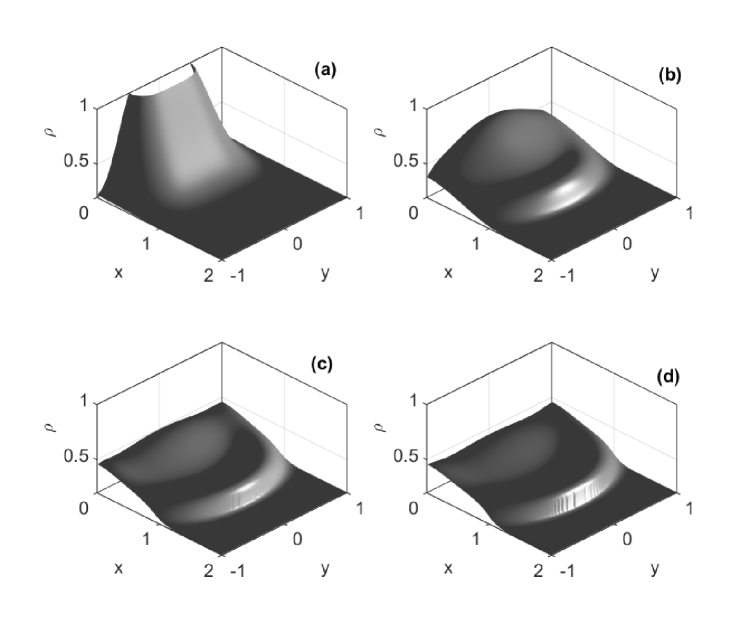
Figure 2: Time evolution of the density, as described by the compressible Euler equation at $t=0$ (a), $t=0.4$ (b), $t=0.511$ (c), and $t=0.55$ (d). The initial condition is a concentrated density in an initially quiescent fluid, as given in (49). At (c), a shock forms, which has spread in (d).

We are interested in describing the formation of a singularity in solutions of the compressible Euler equation. At the point where the singularity first forms, the gradients of all variables $\rho,u,v$ blow up, while the variables themselves remain finite. In the generic case, the singularity develops at a point (the gradient blowing up along a line corresponds to a non-generic initial condition); we denote the conditions at this point (such as the density $\rho_{0}$ or the velocity $\boldsymbol{v}_{0}=(u_{0},v_{0})$) with the subscript zero. We assume that at the critical time $t_{0}$ the gradient $\nabla u$ blows up at one point $(x_{0},y_{0})$ in all directions of the $(x,y)$ plane except one, in which it remains bounded. By contrast, a gradient blowing up in all directions corresponds to an elliptic umbilic singularity, typical of elliptic systems.

Using the invariance of the Euler equation under rotation in the $(x,y)$- plane, we denote the direction where the gradient of $u$ remains bounded at the critical point by $y$, while $\partial x/\partial u=0$. Since the flow is potential, it follows that the first derivative $v_{x}=u_{y}$ remains bounded at the singular point. The condition that the profile has not already overturned amounts to demanding that $\partial^{2}x/\partial u^{2}=0$, while the third derivative will in general be finite ([23], [25]). Thus in summary at the point of the wave profile first becoming singular we have the conditions

$$\frac{\partial u}{\partial y}=const,\quad\frac{\partial x}{\partial u}=0,\quad\frac{\partial^{2}x}{\partial u^{2}}=0,\quad\frac{\partial^{3}x}{\partial u^{3}}=const.$$ (5)

This is illustrated in Fig. 2, which shows an example of a numerical simulation of the Euler equation to be described in more detail in Section 5. It starts from a smooth initial condition for the density, whose profile gradually steepens, until a shock is formed at a point $(x_{0},y_{0}=0)$ at the time $t=t_{0}$ (panel (c)). For $t>t_{0}$, the shock spreads along a line transversal to the direction of propagation (in the $x$-direction), while the height of the jump increases.

We move into a frame of reference such that

$${\bf v}_{0}\equiv(u_{0},v_{0})=0$$

at the point where the singularity is formed. The speed of sound at the singular point is

$$c_{0}^{2}=\frac{\partial p}{\partial\rho}=A\rho_{0}^{\gamma-1}.$$ (6)

To describe the neighborhood of the singularity, we use a self-similar description ([16]), in analogy to caustic singularities in two dimensions ([17]), and shocks in the dKP equation ([19]).

In the self-similar region, we assume the scalings $x^{\prime}\propto t^{\prime\beta_{1}}$, $y^{\prime}\propto t^{\prime\beta_{2}}$, and $u\propto t^{\prime\alpha}$, where $x^{\prime}=x-x_{0}$, $y^{\prime}=y-y_{0}$, and $t^{\prime}=t_{0}-t$, so that $t^{\prime}>0$ before the singularity, and $t^{\prime}<0$ after. Balancing the first two terms in the Euler equation (3) in the propagation direction, we obtain $\alpha-1=2\alpha-\beta_{1}$. If in analogy to (5) we demand $\partial^{3}x/\partial u^{3}=const$, we have $3\alpha=\beta_{1}$, so that $\alpha=1/2$ and $\beta_{1}=3/2$. Moving in the transversal ($y$) direction, the blow-up of the gradient will occur at a slightly later time $t_{c}(y^{\prime})-t_{0}=ay^{\prime 2}+O(y^{3})\propto t^{\prime}$; the linear term must vanish, since otherwise there would be a $y^{\prime}\neq 0$ where blow-up would occur at a time earlier than $t_{0}$. Hence it follows that $\beta_{2}=1/2$. The scaling exponents correspond to those found previously for wave breaking ([29],[30]), the cusp caustic ([17]), and for shock formation in two dimensions ([19]).

Since the shock travels on the back of a sound wave with speed $c_{0}$ in the $x$-direction, we consider the ansatz

$$\begin{split}&\phi(x,y,t)=|t^{\prime}|g_{2}(\eta)+|t^{\prime}|^{\frac{3}{2}}g_{1}(\eta)+|t^{\prime}|^{2}\Phi(\xi,\eta)+|t^{\prime}|^{\frac{5}{2}}\Phi_{1}(\xi,\eta)+\dots\\ &\xi=\frac{x^{\prime}+c_{0}t^{\prime}-c_{1}y^{\prime}-By^{\prime 2}}{|t^{\prime}|^{3/2}},\quad\eta=\frac{y^{\prime}}{|t^{\prime}|^{1/2}}\end{split}$$ (7)

for the potential. Observe that

$$u(x,y,t)=\phi_{x}(x,y,t)=|t^{\prime}|^{\frac{1}{2}}\Phi_{\xi}(\xi,\eta)+O(|t^{\prime}|):=|t^{\prime}|^{\frac{1}{2}}U(\xi,\eta)+O(|t^{\prime}|)$$ (8)

$$v=\phi_{y}=|t^{\prime}|^{\frac{1}{2}}(g_{2\eta}-c_{1}\Phi_{\xi})+|t^{\prime}|(g_{1\eta}-2B\eta\Phi_{\xi})+O(|t^{\prime}|^{\frac{3}{2}}).$$

As in ([17]), $-c_{1}y^{\prime}-By^{\prime 2}$ in $\xi$ is a lower order term, which describes a modulation in the transversal direction. A third order term in $y$ would be proportional to $\eta^{3}$, which is already accounted for in the $\eta$ dependence of $\Phi$. The absolute sign guarantees that (7) works both before and after the singularity. For the density we make the ansatz

$$\rho(x,y,t)=\rho_{0}\left[1+|t^{\prime}|^{1/2}R(\xi,\eta)+|t^{\prime}|Q(\xi,\eta)\right]+O(t^{\prime 3/2}),$$ (9)

which solves (2) and (4) to leading order, as we will see now. The higher order contributions $\Phi_{1}$ and $Q$ are needed for consistency, but we will not calculate them here.

Inserting (7),(9) into (4), we obtain

$$\begin{split}&\pm(\dfrac{1}{2}g_{2\eta}\eta-g_{2})+|t^{\prime}|^{1/2}\left(\pm\dfrac{1}{2}(g_{1\eta}\eta-3g_{1})-c_{0}\Phi_{\xi}\right)+\\ &|t^{\prime}|\left[\mp 2\Phi\pm\frac{3\xi}{2}\Phi_{\xi}\pm\frac{\eta}{2}\Phi_{\eta}+\frac{1}{2}\Phi_{\xi}^{2}+\dfrac{1}{2}(g_{2\eta}-c_{1}\Phi_{\xi})^{2}-c_{0}\Phi_{1\xi}\right]=\\ &-c_{0}^{2}\left\{|t^{\prime}|^{1/2}R+|t^{\prime}|[Q+\frac{1}{2}(\gamma-2)R^{2}]\right\}+O(t^{\prime 3/2}).\end{split}$$ (10)

Thus at order $|t^{\prime}|^{0}$ and $|t^{\prime}|^{\frac{1}{2}}$ we have

$$\dfrac{\eta}{2}g_{2\eta}=g_{2},$$ (11)

$$c_{0}R=\Phi_{\xi}\mp\dfrac{1}{2c_{0}}(g_{1\eta}\eta-3g_{1})=U(\xi,\eta)\mp\dfrac{1}{2c_{0}}(g_{1\eta}\eta-3g_{1}).$$ (12)

Equation (11) gives

$$g_{2}(\eta)=a_{0}\eta^{2},$$

for some constant $a_{0}$. Since we expect the leading order term, $R(\xi,\eta)$, of $\rho$ to be continuous in the transversal direction $y$ near the singularity point, we infer from (12) that

$$g_{1\eta}\eta-3g_{1}=0,$$ (13)

so that one has

$$c_{0}R=\Phi_{\xi}=U(\xi,\eta),\quad g_{1}(\eta)=a_{1}\eta^{3}$$ (14)

for some constant $a_{1}$. Finally grouping together terms of order $|t|^{\prime}$ in (10) and using (14), we obtain

$$c_{0}^{2}Q=\pm 2\Phi\mp\frac{3\xi}{2}\Phi_{\xi}\mp\frac{\eta}{2}\Phi_{\eta}+\frac{1}{2}(1-\gamma)\Phi_{\xi}^{2}-\dfrac{1}{2}(g_{2\eta}-c_{1}\Phi_{\xi})^{2}+c_{0}\Phi_{1\xi}\,.$$ (15)

Next, inserting (7),(9) into (2), we have

$$-c_{0}R_{\xi}|t^{\prime}|^{-1}+|t^{\prime}|^{-1/2}\left[\mp\frac{R}{2}\pm\frac{3\xi}{2}R_{\xi}\pm\frac{\eta}{2}R_{\eta}-c_{0}Q_{\xi}\right]+|t^{\prime}|^{-1}(1+c_{1}^{2})\Phi_{\xi\xi}$$

$$+|t^{\prime}|^{-1/2}\left[\Phi_{\xi}R_{\xi}+\Phi_{\xi\xi}R+4c_{1}B\eta\Phi_{\xi\xi}-c_{1}(g_{2\eta}-c_{1}\Phi_{\xi})R_{\xi}+\Phi_{1\xi\xi}\right]=O(t^{\prime 0}),$$

whose leading order part is compatible with (12) if

$$c_{1}=0.$$ (16)

The next order, combined with (12), gives

$$c_{0}^{2}Q_{\xi}=\mp\frac{\Phi_{\xi}}{2}\pm\frac{3\xi}{2}\Phi_{\xi\xi}\pm\frac{\eta}{2}\Phi_{\xi\eta}+2\Phi_{\xi}\Phi_{\xi\xi}+c_{0}\Phi_{1\xi\xi}\,.$$ (17)

Differentiating (15) with respect to $\xi$ and subtracting (17) one obtains

$$\Phi_{\xi}-3\xi\Phi_{\xi\xi}-\eta\Phi_{\eta\xi}=\pm(\gamma+1)\Phi_{\xi}\Phi_{\xi\xi},$$ (18)

which is a closed equation for $\Phi$. Summing (15) with the integral of (17) with respect to $\xi$ results in

$$c_{0}^{2}Q=\frac{3-\gamma}{4}U^{2}-\dfrac{a_{0}}{2}\eta^{2}+2c_{0}\Phi_{1\xi},$$ (19)

where the scaling function $\Phi_{1}$ is left undetermined at the present level of approximation. Therefore, we have not made explicit the constant of integration in (19).

Using (14) and the above relation we can express the density $\rho$ in (9) has

$$\rho=\rho_{0}\left[1+\frac{|t^{\prime}|^{1/2}}{c_{0}}U(\xi,\eta)+\frac{3-\gamma}{4c_{0}^{2}}|t^{\prime}|U^{2}(\xi,\eta)\right]+|t^{\prime}|\rho_{0}\left[2c_{0}\Phi_{1}(\xi,\eta)-\dfrac{a_{0}}{2}\eta^{2}\right]+O(t^{\prime 3/2}).$$ (20)

Note that this means that

$$\rho=\rho_{0}\left[1+\frac{\gamma-1}{2c_{0}}u\right]^{2/(\gamma-1)}+O(|t^{\prime}|),$$ (21)

which, up to terms of order $O(|t^{\prime}|),$ is the form of a simple wave ([23]) for the one-dimensional Euler system. In the limit $\gamma\to 1$ one obtains

$$\rho=\rho_{0}e^{\frac{u}{c_{0}}}+O(|t|^{\prime}),$$

which is also consistent with the form of a simple wave in the case $\gamma=1$.

The case of a Karman-Tsien gas [6] $\gamma=-1$ is special. This is because the structure of the similarity solution is different, and (7) is to be replaced by $\xi=(x^{\prime}-By^{\prime 2})/t^{\prime 3/2}$. In this solution, the pressure is subdominant, so one is effectively solving the kinematic equation.

Remark 3.1

After setting

$$h(\xi,\eta)=-\frac{\gamma+1}{2}\Phi(\xi,\eta)$$

in equation (18) and integrating in $\xi$ one obtains

$$4h-3\xi h_{\xi}-\eta h_{\eta}\pm h_{\xi}^{2}=0,$$ (22)

which is the similarity equation derived for solutions of the eikonal equation ([17]).

Finally to solve (18), we put $U=\Phi_{\xi}$ to obtain

$$U-3\xi U_{\xi}-\eta U_{\eta}=\pm(\gamma+1)UU_{\xi},$$ (23)

which can be linearized by transforming to $\xi(U,\eta)$:

$$\xi_{U}U-3\xi+\eta\xi_{\eta}=\pm(\gamma+1)U,$$ (24)

with general solution

$$\xi=\mp\frac{\gamma+1}{2}U-U^{3}F\left(\frac{\eta}{U}\right).$$ (25)

The form of the function $F=F(z)$ is set by the requirement that the similarity profile must be regular. From (25) we find that

$$\frac{\partial^{4}\xi}{\partial\eta^{4}}=-\dfrac{1}{U}F^{(iv)}\left(\frac{\eta}{U}\right),$$

so by putting $\eta=aU$ for $a\neq 0$, and letting $U\rightarrow 0$, one needs to impose $F^{(iv)}(a)=0$ for any nonzero constant $a$. Hence $F$ is a cubic polynomial, namely

$$F(z)=A_{0}+A_{1}z+A_{2}z^{2}+A_{3}z^{3},$$ (26)

and the similarity profile is

$$\xi=\mp\frac{\gamma+1}{2}U-A_{0}U^{3}-A_{1}U^{2}\eta-A_{2}U\eta^{2}-A_{3}\eta^{3},$$ (27)

for some constants $A_{0},A_{1},A_{2}$ and $A_{3}$.

In principle one could use different values of these constants for $t^{\prime}>0$ and $t^{\prime}<0$. However, we observe that for fixed values of $x^{\prime}$ and $y^{\prime}$ away from $(0,0)$ the local structure of the solution has to be single-valued as a function of $t^{\prime}$ as $|t|^{\prime}\to 0$. It follows that $U(\xi,\eta)$ has to be a single-valued function of $\xi$ and $\eta$ as $\xi\to\infty$ and $\eta\to\infty$, which is possible only if the constants $A_{0},A_{1},A_{2}$ and $A_{3}$ have the same values before and after the singularity.

This completes the solution; constraints on the coefficients $A_{i}$ are given in (40) below. It is easy to confirm that the conditions (5) are satisfied. Note that (27) corresponds exactly to the generic form of a cusp singularity ([17, 19]) also found in the catastrophe theory of optical caustics ([28]). In particular, there are no quadratic terms in the expansion. From the condition that there can be no overturning of the profile before shock formation (upper sign), we also deduce the condition $A_{0}>0$.

To determine the coefficients $A_{i}$ in (27) numerically, as we will do below, it is useful to take third derivatives of $x$ with respect to $u$ and $y$. First, at constant $y$, we have

$$x_{u}=u_{x}^{-1},$$

and thus

$$x_{uu}=-\frac{u_{xx}}{u_{x}^{3}},\quad x_{uuu}=-\frac{u_{xxx}}{u_{x}^{4}}+3\frac{u_{xx}^{2}}{u_{x}^{5}}.$$ (28)

According to the implicit function theorem,

$$x_{y}=-\frac{u_{y}}{u_{x}},$$

while

$$\left.\frac{1}{\partial y}\right|_{u}f(x,y)=\left.\frac{1}{\partial y}\right|_{u}f(x(u,y),y)=-f_{x}\frac{u_{y}}{u_{x}}+f_{y},$$

and thus

$$x_{yy}=\left(\frac{u_{y}}{u_{x}}\right)_{x}\frac{u_{y}}{u_{x}}-\left(\frac{u_{y}}{u_{x}}\right)_{y}=2\frac{u_{xy}u_{y}}{u_{x}^{2}}-\frac{u_{yy}}{u_{x}}-\frac{u_{xx}u_{y}^{2}}{u_{x}^{3}}$$

and

$$x_{uyy}=\left[2\frac{u_{xy}u_{y}}{u_{x}^{2}}-\frac{u_{yy}}{u_{x}}-\frac{u_{xx}u_{y}^{2}}{u_{x}^{3}}\right]_{x}u_{x}^{-1},$$ (29)

$$x_{uuy}=\left(\frac{u_{xx}}{u_{x}^{3}}\right)_{x}\frac{u_{y}}{u_{x}}-\left(\frac{u_{xx}}{u_{x}^{3}}\right)_{y},$$ (30)

$$x_{yyy}=-\left[2\frac{u_{xy}u_{y}}{u_{x}^{2}}-\frac{u_{yy}}{u_{x}}-\frac{u_{xx}u_{y}^{2}}{u_{x}^{3}}\right]_{x}\frac{u_{y}}{u_{x}}+\left[2\frac{u_{xy}u_{y}}{u_{x}^{2}}-\frac{u_{yy}}{u_{x}}-\frac{u_{xx}u_{y}^{2}}{u_{x}^{3}}\right]_{y}.$$ (31)

Using the scaling (7), the derivatives can be converted to similarity variables, so from (27) one obtains

$$A_{0}\simeq-\frac{x_{uuu}}{6},\quad A_{1}\simeq-\frac{x_{uuy}}{2},\quad A_{2}\simeq-\frac{x_{uyy}}{2},\quad A_{3}\simeq-\frac{x_{yyy}}{6},$$ (32)

to be evaluated at the critical point $t=t_{0}$, $x=x_{0}$ and $y=y_{0}$. Here and below, we are assuming that the higher order scaling functions which appear in (7) are regular, so that the higher order contributions to to $u$ in (8) become negligible near the critical point.

Finally, the constant $B$ in (7) can be evaluated by computing the second derivative with respect to $y$:

$$u_{yy}\simeq 4B^{2}\eta^{2}|t^{\prime}|^{-3/2}U_{\xi\xi}-2B|t^{\prime}|^{-1}U_{\xi}+|t^{\prime}|^{-1/2}U_{\eta\eta}.$$

Thus at $\eta=\xi=0$, using $U_{\xi}=\xi_{U}^{-1}=\mp 2/(\gamma+1)$, $U_{\xi\xi}=0$ and $U_{\eta\eta}=0$, one finds that

$$B\simeq\frac{\gamma+1}{4}u_{yy}(t_{0}-t)$$ (33)

as $t^{\prime}\rightarrow 0$. Summarizing, the solution near the singularity at the point $(x_{0},y_{0},t_{0})$ in the physical variables $x^{\prime}=x-x_{0}$, $y^{\prime}=y-y_{0}$ and $t^{\prime}=t_{0}-t$ takes the form

$$x^{\prime}-c_{0}t^{\prime}-By^{\prime 2}\simeq-\dfrac{\gamma+1}{2}t^{\prime}u-A_{0}u^{3}-A_{1}u^{2}y^{\prime}-A_{2}uy^{\prime 2}-A_{3}y^{\prime 3},$$ (34)

where the constant $A_{0},A_{1},A_{2}$ and $A_{3}$ are determined in (32) and the constant $B$ is determines in (33).

Remark 3.2

We claim that the local structure of the singularity for the velocity $u(x,y,t)$ is captured by the self-similar profile obtained in (34). This represents the leading order term in the multiple scale expansion of $u(x,y,t)=|t^{\prime}|^{\frac{1}{2}}U(\xi,\eta)+O(|t^{\prime}|)$. We will support this claim by a numerical example presented in Sect. 5. Furthermore, if we assume that the higher order corrections to the potential field are regular at the singular point, one can deduce that the gradient of $u$ with respect to $y$ is not only constant but zero at the singular point. This fact is certainly true for smooth initial data that are invariant with respect to the symmetry $y\to-y$.

4 After the singularity

After a shock occurs, the adiabatic law (1) is no longer valid, since entropy is generated inside the shock front, the entropy being given by

$$s=c_{v}\ln\frac{p}{\rho^{\gamma}},$$ (35)

where $c_{v}$ is the specific heat, which for simplicity we consider constant. However, the jump in entropy across the shock is only of order $|t^{\prime}|^{3/2}$, which results in a subleading contribution to (10). Following ([23]), and using

$$w=\frac{\gamma}{\gamma-1}\frac{p}{\rho}$$

for the enthalpy of a polyatomic gas, the Rankine-Hugoniot jump condition across a shock in a frame of reference moving with the shock is

$$\frac{\gamma}{\gamma+1}\left(\frac{p_{1}}{\rho_{1}}-\frac{p_{2}}{\rho_{2}}\right)+\frac{1}{2}\left(\frac{1}{\rho_{1}}+\frac{1}{\rho_{2}}\right)\left(p_{2}-p_{1}\right)=0,$$ (36)

where the index 1 denotes the front of the shock, index 2 the back. Combining (35) and (36), and expanding in the size of the pressure jump $p_{2}=p_{1}+\Delta p$, one finds

$$\Delta s\equiv s_{2}-s_{1}=\frac{c_{v}}{12}\frac{\gamma^{2}-1}{\gamma^{2}}\frac{\Delta p^{3}}{p_{1}^{3}}.$$ (37)

Thus the jump in entropy is only of third order, which a fact which remains true for a gas of arbitrary thermodynamic properties ([23]).

From the solution (9), we have that $\Delta p\propto t^{\prime 1/2}$, and so it follows that $\Delta s\propto t^{\prime 3/2}$, which means that

$$p=\frac{A}{\gamma}\rho^{\gamma}+O(t^{\prime 3/2}).$$

Clearly, this makes a contribution of order $t^{\prime 3/2}$ to (10), which can be neglected. Given the leading-order solution, one can use the entropy production (37) to calculate the distribution of entropy near the shock, using the convection equation

$$\left(\frac{p}{\rho^{\gamma}}\right)_{t}+{\bf v}\cdot\nabla\left(\frac{p}{\rho^{\gamma}}\right)=0,$$ (38)

which says that entropy is transported with each fluid element, but not produced outside of the shock.

4.1 Shock condition

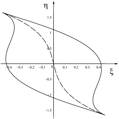
Figure 3: The lip-shaped region inside which the velocity profile overturns; parameters are chosen arbitrarily as $(A_{0},A_{1},A2,A3)=(2,0.3,0.5,0.1)$ and $\gamma=5/3$. The dashed line marks the position of the shock.

After the singularity, the solution given by (27) has a region where the profile has overturned. The line along which the profile is vertical is given by $\partial\xi/\partial U=0$, and thus for $t>t_{0}$:

$$\frac{\gamma+1}{2}=3A_{0}U^{2}+2A_{1}U\eta+A_{2}\eta^{2}.$$ (39)

This can be parameterized as an ellipse in $(U,\eta)$-space, provided that the quadratic form on the right is positive definite; for this we need that

$$A_{0}>0,\quad 3A_{0}A_{2}-A_{1}^{2}>0.$$ (40)

If the conditions (40) were not met, (39) would not describe a closed curve, but instead extend to infinity. This is unphysical, since it would imply that the shock has spread an infinite distance. As the ellipse (39) is inserted into (27), one obtains a closed lip-shaped region, an example of which is shown in Fig. 3. In the case $A_{1}=A_{3}=0$, namely for initial data with a symmetry with respect to reflection on the $y$-axis one has

$$\xi=\pm\dfrac{2}{3\sqrt{3A_{0}}}\left(\dfrac{\gamma+1}{2}-A_{2}\eta^{2}\right)^{\frac{3}{2}}.$$

The lip describes how the overturned region (and thus the shock) spreads in space, and corresponds to similar results found in ([17]) and ([19]).

To find the position of the shock, we transform the solution (27) to a form equivalent to that of the one-dimensional case. Namely, we can introduce shifted variables

$$\bar{\xi}=\xi-\xi_{s}(\eta),\quad\bar{U}=U-U_{s}(\eta),$$ (41)

so that (27) becomes

$$\bar{\xi}=-A_{0}\bar{U}\left(\bar{U}^{2}-\Delta^{2}(\eta)\right).$$ (42)

Comparing coefficients, we obtain

$$U_{s}=-\frac{A_{1}}{3A_{0}}\eta,\quad\xi_{s}=-\frac{A_{1}(\gamma+1)}{6A_{0}}\eta+\frac{9A_{0}A_{1}A_{2}-2A_{1}^{3}-27A_{0}^{2}A_{3}}{27A_{0}^{2}}\eta^{3},$$ (43)

$$\Delta=\sqrt{\frac{\gamma+1}{2A_{0}}+\frac{A_{1}^{2}-3A_{0}A_{2}}{3A_{0}^{2}}\eta^{2}}.$$ (44)

The lateral width of the shock is determined from the condition that $\Delta=0$, and thus

$$\eta_{\pm}=\pm\sqrt{\frac{3A_{0}(\gamma+1)}{6A_{0}A_{2}-2A_{1}^{2}}},$$ (45)

where (40) guarantees that this is well-defined. Clearly, in real space the width of the shock increases like $|t^{\prime}|^{1/2}$.

Having written the profile in the form of a simple s-curve (42), if follows from symmetry that the shock must be at $\bar{\xi}=0$, so that the shock position is at $\xi_{s}(\eta)$. This is the dashed line plotted in Fig. 3. The line $\bar{\xi}=0$ intersects (42) at $\bar{U}=\pm\Delta$, and so the velocities at the front and back of the shock are $U_{1}=U_{s}-\Delta$ and $U_{2}=U_{s}+\Delta$, respectively, so that the size of the jump is $2\Delta$.

In real space the shock position is at

$$\begin{split}x_{s}^{\prime}&=-c_{0}t^{\prime}+By^{\prime 2}+|t^{\prime}|^{3/2}\xi_{s}(\eta)\\ &=By^{\prime 2}-\left(c_{0}-\frac{A_{1}(\gamma+1)}{6A_{0}}y^{\prime}\right)t^{\prime}+\frac{9A_{0}A_{1}A_{2}-2A_{1}^{3}-27A_{0}^{2}A_{3}}{27A_{0}^{2}}y^{\prime 3},\end{split}$$ (46)

so that the shock speed in the $x$-direction is

$$u_{s}=c_{0}-\frac{A_{1}(\gamma+1)}{6A_{0}}y^{\prime};$$ (47)

the speed in the $y$-direction is of lower order.

To confirm that (47) is in agreement with the Rankine-Hugoniot conditions at the shock, note that according to (42), the fluid velocities at the back and the front of the shock are

$$u_{1/2}=|t^{\prime}|^{1/2}\left(U_{s}\pm\Delta\right).$$ (48)

Using mass conservation, the shock velocity is ([23])

$$u_{s}=\frac{\rho_{1}u_{1}-\rho_{2}u_{2}}{\rho_{1}-\rho_{2}},$$

which to leading order can be written as

$$u_{s}=\left.\frac{\partial\rho u}{\partial\rho}\right|_{u=(u_{1}+u_{2})/2}=\frac{u_{1}+u_{2}}{2}+\rho\left.\left(\frac{\partial u}{\partial\rho}\right)^{-1}\right|_{u=(u_{1}+u_{2})/2}=c_{0}+\frac{\gamma+1}{4}\left(u_{1}+u_{2}\right),$$

where in the last step we used (21). Combining this with (48) and the expression for $U_{s}$, one indeed recovers (47). It is straightforward to check that the other Rankine-Hugoniot conditions are satisfied identically to leading order.

5 Numerical simulation

We test the results of the preceding sections by direct numerical simulation of the Euler equation. Starting from a smooth initial condition for the density and the velocity, a shock develops. Our aim is to compare to the similarity profile (27), both before and after shock formation, and to confirm the self-similar properties of the solution, as described by (7),(9). We have seen in earlier work ([19]) that it is much easier to test self-similar properties of profiles after the singularity, where they have more structure. We will pursue this idea but with the additional twist that we use (32) before the singularity to calculate the coefficients $A_{0}-A_{3}$, which determines the self-similar solution completely. We are then able to predict profiles after the singularity without any adjustable parameters.

We begin with the initial condition

$$\rho(x,y,0)=0.2+e^{-4x^{4}-4y^{2}},\quad{\bf v}(x,y,0)=0,$$ (49)

which corresponds to a localized high-density, high-pressure region (as if generated by an explosion), starting from rest. We choose the adiabatic exponent of air $\gamma=7/5$, and $A=\gamma$ in the ideal gas law (1). The initial condition was chosen such that gradients are steeper in the $x$-direction, so that a shock first occurs on the $x$-axis. Further, the solution is symmetric about the $x$-axis, so that the coefficients $A_{1}$ and $A_{3}$ in the self-similar solution (27) vanish. This makes it much easier to spot the singularity; in particular, the $x$ and $y$ axes of the simulation are the same as those defined by the gradients of the density, in that $\partial\rho/\partial y=0$ is satisfied.

For times $t<t_{0}$ we use both a finite difference scheme and a Fourier pseudo-spectral method to solve the equations. In the finite-difference scheme, the equations are written as in (1)-(3), and are discretized in space using fourth order finite differences on a uniform mesh in the numerical domain $[0,2]\times[0,2]$. Mirror symmetry is applied at $x=0$ and at $y=0$, while outflow conditions (vanishing derivatives of all variables) are applied at $x=2$ and at $y=2$. An explicit second order Runge-Kutta scheme is used to advance the solution in time. We used $2000\times 2000$ points in space and a fixed time step of $\Delta t=1.25\cdot 10^{-4}$.

For the pseudospectral method ([7]), (2) and (4) are set in a $[-2\pi,2\pi]\times[-2\pi,2\pi]$ box with periodic boundary conditions, with an equispaced collocation grid of resolution $2^{14}\times 2^{14}$. The time discretization is obtained by means of a standard fourth order explicit Runge-Kutta scheme with $\delta t=5\cdot 10^{-5}$. To remove aliasing errors, we adopt a filtering as described in [20], whereby Fourier coefficients are multiplied by the exponential function

$$\sigma(k)=\exp(-36(|k|/N)^{36}),$$ (50)

where $N=2^{14}$ is the number of Fourier modes in each direction.

As the singularity is approached, steepening gradients require higher and higher Fourier modes to represent profiles accurately. To guarantee sufficient resolution as the profiles steepen, we inspect the magnitude of the Fourier coefficients at each time step. As long as all Fourier modes with magnitude higher than the machine epsilon ($10^{-12}$) are represented, the approximation is deemed acceptable; if this is no longer the case for a given resolution, we stop the simulation.

As an example, in Fig. 4 we report the spectrum for an acceptable solution (at time $t=0.45$) on the left, and for a rejected solution (at time $t=0.48$) on the right. On the left, Fourier amplitudes plateau to the smallest representable number $10^{-12}$, and thus the simulation can be trusted to within the arithmetic precision of the calculation, while on the right this is no longer the case. On the basis of this, we continue the pseudospectral calculation up to $t=0.46$, and perform a least squares interpolation of this part of the solution to extrapolate to the critical time.

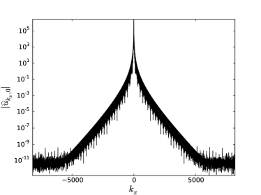
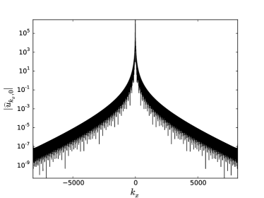
Figure 4: Magnitude of Fourier coefficients of the numerical solution as function of the $x$-wavenumber at the origin of the $y$-wavenumber axis. At $t=0.45$ (left) there is sufficient resolution, while at $t=0.48$ (right) the spectrum has been rejected.

When a shock appears, we need to use a finite difference method that remains stable even in the presence of jumps of the hydrodynamic fields. To this end, the equations are written in conservative form, where the fluxes are computed using the second-order-in-space central-upwind scheme (see e.g. Section 3.1 of ([22]) with slope limiting ([van Leer(1979)]). In addition to $\rho$ and the mass flux ${\bf j}=\rho{\bf v}$, the method uses the internal energy $e=\rho{\bf v}^{2}/2+p/(\gamma-1)$ as an additional variable. The energy follows the conservation equation

$$\frac{\partial e}{\partial t}+\nabla\cdot({\bf v}(e+p))=0,$$ (51)

while (2) and (3) are solved as before, but in conservative form. Energy dissipation occurs within a tiny region around the shock, where entropy is created. This method remains stable even if the shock is not resolved, effectively modeling non-classical solutions to the Euler equation, which satisfy the Rankine-Hugoniot conditions. Time integration is performed with a generic variable time-step predictor-corrector scheme.

This numerical scheme is implemented using the “Basilisk” software, developed by S. Popinet. It uses Quadtrees ([31]) to allow efficient adaptive grid refinement in the region where the gradient of the density or of the velocity becomes large. Linear refinement is used on the trees, so that reconstructed values also use slope limiting. The numerical domain is $[-2,2]\times[-2,2]$, i.e. symmetry conditions are not applied in this case, and it is discretized using $2^{10}\times 2^{10}$ points initially. The resolution is adapted at each time step according to the (wavelet-estimated) discretization error of the density field. Whenever the discretization error is larger than $5\times 10^{-3}$, the mesh is refined, down to a prescribed maximum quadtree level. Several simulations have been carried out by varying the maximum level of refinement from 10 to 18.

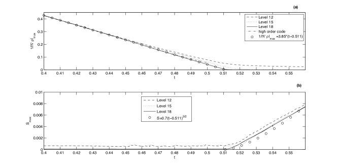
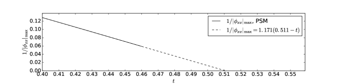
Figure 5: The inverse of the maximum of the density gradient (top), and the maximum of the entropy (center) over the whole domain as function of time, for three different levels of resolution, using the Basilisk code for the compressible Euler equation. The dot-dashed line is the result of the fourth-order code, up to $t=0.5$. By fitting to the predicted linear law (52), we get an accurate prediction for the singularity time $t_{0}=0.511$. In the bottom panel, the inverse of the maximum of $\phi_{xx}$, obtained using the pseudospectral method, is plotted as a function of time. A linear fit leads $t_{0}=0.512$.

To locate the singularity, we look at the maximum gradient of the density $\rho$ and the velocity field $u$, which is in the $x$-direction:

$$\frac{\partial\rho}{\partial x}=\frac{\rho_{0}}{c_{0}}|t^{\prime}|^{-1}U_{\xi},\quad u_{x}=|t^{\prime}|^{-1}U_{\xi}.$$

According to the similarity solution (27), the minimum $\xi_{U}=-(\gamma+1)/2$ is at $U=\eta=0$, and hence

$$\left|{\boldsymbol{\nabla}}\rho\right|_{max}^{-1}=\frac{c_{0}}{\rho_{0}}\frac{1+\gamma}{2}|t^{\prime}|,\quad\left|u_{x}\right|_{max}^{-1}=\frac{1+\gamma}{2}|t^{\prime}|.$$ (52)

The predicted linear dependence for $t<t_{0}$ is confirmed in Fig. 5 (top and bottom). The quantity $\left|{\boldsymbol{\nabla}}\rho\right|_{max}^{-1}$ is computed using the conservative scheme, since it allows us to go up to the singularity and beyond. Close to the singularity, the maximum gradient of the density crosses over to a finite value, as the scheme can no longer resolve the steepest gradient. As the resolution is increased, the linear behavior continues to smaller values. From a linear fit of the inverse of $\rho_{x}$ to the highest resolution data (circles), we find $t_{0}=0.511$, which is our most accurate estimate of the singularity time, since it is based on a simulation which continues up to shock formation and beyond. Using (52), the prefactor of the linear fit is $4.01$, in reasonable agreement with the fitted value of $3.85$. The linear fit also agrees very well with the result of the fourth order finite-difference code before the singularity.

To confirm that the velocity component $u$ blows up in the same way as $\rho$, we use the pseudospectral method to also calculate $\left|u_{x}\right|_{max}^{-1}$. A linear fit to $\left|u_{x}\right|_{max}^{-1}=|\phi_{xx}|_{max}^{-1}$ gives a singularity time of $0.512$, in good agreement with the result of the finite difference scheme. The prefactor of the linear fit is $1.171$, again in good agreement with the theoretical value $(\gamma+1)/2=1.20$ (see bottom of Fig. 5).

Using the location of the maximum gradient of $\rho$ at $t_{0}$, we obtain ${\bf x}_{0}=(1.4052,0)$ as the position of the singularity. At this point, the velocity ${\bf v}_{0}=(0.2769,0)$, the density $\rho_{0}=0.2731$, and $c_{0}=0.9127$. From now on, we will report all results in a frame of reference which moves with ${\bf v}_{0}$, and relative to ${\bf x}_{0}$. The middle graph of Fig. 5 shows the maximum entropy, which starts to grow exactly at the time of shock formation $t_{0}$. The growth is consistent with a fit based on (37), which would predict the maximum entropy to grow like $t^{\prime 3/2}$. However, our results are not sufficiently accurate to distinguish this from a linear behavior.

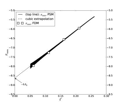
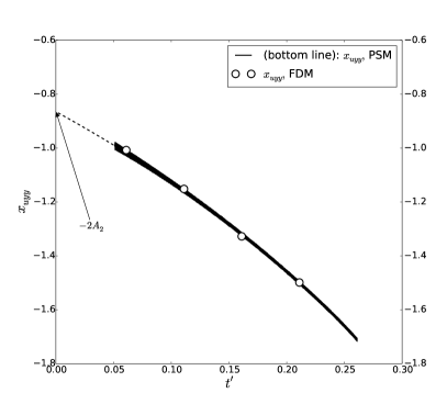
Figure 6: The derivatives $x_{uuu}$ (left) and $x_{uyy}$ (right) as function of $t^{\prime}$ for the initial conditions (49), evaluated at the maximum of the pressure, using the PseudoSpectral Method (PSM) and the Finite Difference Method (FDM). The values of$x_{uuu}$ and $x_{uyy}$ are plotted before they start to oscillate strongly for $t^{\prime}<0.05$. The coefficients $A_{0}$ and $A_{2}$ are found by extrapolating to $t^{\prime}=0$.

[capbesideposition=right,top, capbesidewidth=4cm]figure[]

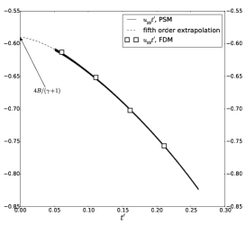
Figure 7: Plot of the values of $u_{yy}t^{\prime}$ for several values of $t^{\prime}$ using PSM and FDM. The coefficient $B$ is found from (33) by extrapolating to $t^{\prime}=0$.

	FDM linear extrapolation	PSM	extrapolation
$A_{0}$	$1.5508$	$1.43614$	cubic
$A_{2}$	$0.3328$	$0.43242$	cubic
$B$	-0.33	$-0.35377$	quintic

Table 1: The parameters of the similarity solution as determined numerically from $t<t_{0}$, extrapolating to $t_{0}=0.511$, using the finite difference and pseudospectral methods.

We are now in a position to calculate the constant $B$ (cf. (7) as well as the coefficients $A_{i}$ which appear in the similarity solution (27); by symmetry, $A_{1}=A_{3}=0$. For the latter, We use (32), aiming to evaluate the right-hand sides as close to the singularity as possible. As illustrated in Figs. 6 and 7, and recorded in Table 1), we use the results of both the the finite difference method (FDM) and our pseudo-spectral method (PSM) to extrapolate to $t_{0}$. As seen from (28)-(31), the numerical approximation for the third derivatives will loose resolution eventually, since for example $u_{x}$ blows up at the singularity, and cancellation errors become large. In calculating $x_{uuu}$ and $x_{uyy}$, we use that odd derivatives with respect to $y$ vanish on account of symmetry. We then evaluate $x_{uuu}$ and $x_{uyy}$ at the maximum of the pressure, and plot the result as a function of time see, Fig. 6. We use linear and cubic approximations to extrapolate $x_{uuu}$ and $x_{uyy}$ to $t^{\prime}=0$, from which $A_{0}$ and $A_{2}$ are calculated using (32) (see Table 1). The coefficient $B$ (cf. (7)), is found from (33) by extrapolating to $t=t_{0}$, using both linear and quintic approximations (see Fig. 7 and Table 1). As seen in Table 1), the numerical values for the coefficients, obtained by different methods, are in good agreement

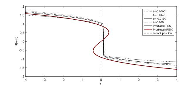
Figure 8: Velocity profiles $u(x,y=0,t)$, rescaled according to (53), for $t^{\prime}$ as given. The heavy line as well as the red line with dots correspond to (27) for $\eta=0$, using the two sets of coefficients. The jump is predicted to be at $\xi=0$ (heavy dashed line).

From (7), the velocity field $u$ in the direction of propagation along the axis of symmetry is

$$u-u_{0}=|t^{\prime}|^{1/2}U\left(\frac{x^{\prime}+c_{0}t^{\prime}}{|t^{\prime}|^{3/2}},0\right).$$ (53)

In Fig. 8, velocity profiles have been rescaled according to (53), and superimposed for the times shown. Note that no adjustable parameter was used to achieve the collapse, which requires accurate estimates for $x_{0}$ and $u_{0}$, as well as the speed of sound $c_{0}$. Theoretical predictions for the profile (27), based on the coefficients from Table 1, are shown as the heavy black line (FDM), and the red line with dots (PSM), giving almost identical results. The theoretical prediction for the shock position is a jump inserted at $\xi=0$. Although there is no adjustable parameter in the comparison, profiles collapse very well over a wide range of $t^{\prime}$ values, and agree with the theoretical prediction, based on an independent determination of the free parameters.

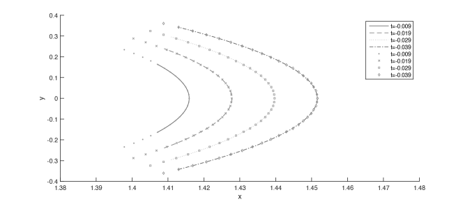
Figure 9: The position of the shock front as function of time, as determined from the maximum of the density gradient. This is superimposed with the theoretical prediction (46), with $B$ as given in Table 1.

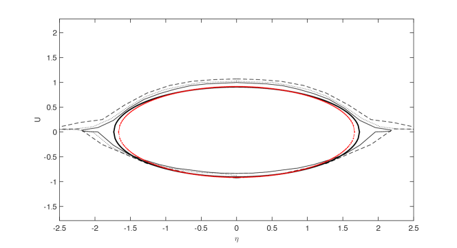
Figure 10: The rescaled values of the velocity field $U_{1,2}$ at the front and back of the shock, written as function of the similarity variable $\eta$. Numerical results are for $t^{\prime}=-0.009$ (dashed line), $t^{\prime}=-0.014$ (dotted line), and $t^{\prime}=-0.039$ (solid line). The heavy solid line and the red line with dots are the theoretical predictions based on (44).

In Figs. 9 and 10 we test the spatial structure of the shock and how it spreads in time. First we show the position of the shock in real space (cf. Fig. 9), as determined from the maximum gradient of the density. This procedure does not determine where the profile has a true jump, so we also have to calculate the height of the jump, for which we use a procedure described below, as applied to the $x$-velocity $u$. We thus see the lateral spreading of the shock as it propagates forward. This is compared to the theoretical prediction (45),(46), with which excellent agreement is found. This confirms that the width of the shock spreads like $|t^{\prime}|^{1/2}$, with a prefactor (45) determined from the coefficients $A_{i}$. It also shows that the shape of the shock front is as predicted by (46).

To look at the structure of the shock in more detail, we consider the velocity in the front and back of the shock, $U_{1/2}=U_{s}\mp\Delta$, as given by (43),(44). This prediction is shown as the heavy black line and the red line with dots in Fig. 10, with coefficients determined before the singularity. The values of $u_{1}$ and $u_{2}$ are determined numerically from slices such as those shown in Fig. 8, but for a range of $y$ values, until the shock disappears. Similarity functions are found by rescaling according to $U_{1/2}=\left(u_{1/2}-u_{0}\right)/|t^{\prime}|^{1/2}$ and $\eta=y^{\prime}/|t^{\prime}|^{1/2}$.

Near the center of the shock, $u_{1}$ and $u_{2}$ are relatively easy to determine, by looking for a corner in profile, where it suddenly becomes vertical; but as the shock becomes weaker near the edge, numerical viscosity leads to a rounding of the jump, and values of $u_{1}$,$u_{2}$ can no longer be read off as easily. Instead, we adopt the following procedure: first, the derivative of the profile has a sharp peak at the position of the shock, which we take as the location of its minimum. Second, we fit a third order polynomial to both the upper and lower branches of the profile, away from the region directly at the shock where numerical viscosity is significant. Then $u_{1}$ is found from the intersection of the upper branch with a vertical line at the position of the shock, and $u_{2}$ from the lower branch. The result of this procedure is shown for three different values of $t^{\prime}$. Again, excellent collapse is found, as well as agreement with the theoretical prediction, based on the two sets of coefficients.

6 Discussion

In this manuscript we have derived the leading order behavior of the solution of the compressible two-dimensional isentropic Euler equation near the formation of its first singularity. We have obtained a self-similar structure for the local solution near the singularity, showing it captures the main features of the local behavior of the shock solution after singularity formation. In particular, we find scaling like $t^{1/2}$ along the orthogonal direction of propagation and scaling like $t^{3/2}$ along the direction of propagation. Furthermore, for a specific choice of initial data, we have compared the spatial structure of the shock with our theoretical predictions, finding good agreement.

It is a worthwhile exercise to extend our calculations to three space dimensions, in which case there are two variables $y$ and $z$ in the direction transversal to the direction of propagation $x$. Repeating essentially the same steps as before, this leads to a similarity profile similar to (27), but which contains all third-order terms in the variables $U$ and the two similarity variables for the transversal directions.

Our similarity solution is in the form of an infinite series (7),(9), of which we calculated the leading order contributions $\Phi(\xi,\eta)$ and $R(\xi,\eta)$. It would be interesting to pursue the calculation to the next order and beyond, in order to calculate the contributions of higher order like $\Phi_{1}(\xi,\eta)$ and $Q(\xi,\eta)$. This will affect the transversal velocity component $v$, while our focus has been on the component $u$ in the direction of propagation.

References

- [1] Alinhac, S. 1993 Temps de vie des solutions régulières des équations d’Euler compressibles. Invent. Math. 111, 627–670.
- [2] Arnold, V. I. 1989 Mathematical methods of classical mechanics, second edition. Springer.
- [3] Arnold, V. I. 1990 Singularities of caustics and wave fronts. Kluwer.
- [4] Berry, M. V. 1981 Singularities in waves and rays. In Les Houches, Session XXXV (ed. R. Balian, M. Kleman & J.-P. Poirier), pp. 453–543. North-Holland: Amsterdam.
- [5] Bianchini, S. & Bressan, A. 2005 Vanishing viscosity solutions of nonlinear hyperbolic systems. Ann. Math. 161, 223–342.
- [6] Bordemann, M. & Hoppe, J. 1993 The dynamics of relativistic membranes. reduction to 2-dimensional fluid dynamics. Phys. Lett. B 317, 315.
- [7] Canuto, C., Hussaini, M. Y., Quarteroni, A. & Zhang, T. 2006 Spectral Methods, , vol. 1. Springer.
- [8] Cates, A. T. & Crighton, D. G. 1990 Nonlinear diffraction and caustic formation. Proc. Roy. Soc. A 430, 69.
- [9] Cates, A. T. & Sturtevant, B. 1997 Shock wave focusing using geometrical shock dynamics. Phys. Fluids 9, 3058.
- [10] Chiodaroli, E. & De Lellis, C. 2015 Global ill-posedness of the isentropic system of gas dynamics. Comm. Pure Appl. Math. 68, 1157–1190.
- [11] Christodoulou, D. 2007 The Formation of Shocks in 3-dimensional Fluids. EMS Monographs in Mathematics.
- [12] Courant, R. & Friedrichs, K. O. 1948 Supersonic flow and shock waves. Springer.
- [13] Cramer, M. S. & Seebass, A. R. 1978 Focusing of weak shock waves at an arête. J. Fluid Mech. 88, 209.
- [14] Dubrovin, B., Grava, T., Klein, C. & Moro, A. 2015 On critical behaviour in systems of hamiltonian partial differential equations. J. Nonlinear Sci. 25, 631–707.
- [15] Eggers, J. & Fontelos, M. A. 2009 The role of self-similarity in singularities of partial differential equations. Nonlinearity 22, R1.
- [16] Eggers, J. & Fontelos, M. A. 2015 Singularities: Formation, Structure, and Propagation. Cambridge University Press, Cambridge.
- [17] Eggers, J., Hoppe, J., Hynek, M. & Suramlishvili, N. 2014 Singularities of relativistic membranes. Geometric Flows 1, 17.
- [18] Elling, V. 2006 A possible counterexample to well posdness of entropy solutions and to godunov scheme convergence. Mathematics of computation 75, 1721 – 1733.
- [19] Grava, T., Klein, C. & Eggers, J. 2016 Shock formation in the dispersionless Kadomtsev–Petviashvili equation. Nonlinearity 29, 1384.
- [20] Hou, T. Y. 2009 Blow-up or no blow-up? A unified computational and analytic approach to 3D incompressible Euler and Navier–Stokes equations. Acta Numerica 18, 277–346.
- [21] Kruzkov, S. N. 1969 Generalized solutions of the Cauchy problem in the large for first order nonlinear equations. Dokl. Akad. Nauk. SSSR 187, 29–32.
- [22] Kurganov, A. & Levy, D. 2002 Central-upwind schemes for the saint-venant system. Mathematical Modelling and Numerical Analysis 36, 397–425.
- [23] Landau, L. D. & Lifshitz, E. M. 1984 Fluid Mechanics. Pergamon: Oxford.
- [24] Lax, P. D. 1972 Hyperbolic Systems of Conservation Laws and the Mathematical Theory of Shock Waves, CBMS Regional Conf. Ser. in Appl. Math., vol. 11. SIAM, Philadelphia.
- [25] Majda, A. 1984 Smooth solutions for the equations of compressible and incompressible fluid flow. In Fluid dynamics (ed. H. Beirão da Veiga), vol. 1047, pp. 75–126. Springer, Berlin.
- [26] Manakov, S. V. & Santini, P. M. 2008 On the solutions of the dKP equation: the nonlinear Riemann Hilbert problem, longtime behaviour, implicit solutions and wave breaking. Nonlinearity 41, 1.
- [27] Manakov, S. V. & Santini, P. M. 2012 Wave breaking in the solutions of the dispersionless Kadomtsev-Petviashvili equation at a finite time. Theoret. and Math. Phys. 172, 1117.
- [28] Nye, J. 1999 Natural Focusing and Fine Structure of Light: Caustics and Wave Dislocations. Institute of Physics Publishing, Bristol.
- [29] Pomeau, Y., Jamin, T., Le Bars, M., Le Gal, P. & Audoly, B. 2008a Law of spreading of the crest of a breaking wave. Proc.Roy. Soc. A 464, 1851–1866.
- [30] Pomeau, Y., Le Berre, M., Guyenne, P. & Grilli, S. 2008b Wave-breaking and generic singularities of nonlinear hyperbolic equations. Nonlinearity 21, T61–T79.
- [31] Popinet, S. 2011 Quadtree-adaptive tsunami modelling. Ocean Dyn. 61, 1261–1285.
- [32] Poston, T. & Stewart, I. 1978 Catastrophe Theory and Its Applications. Dover Publications, Mineola.
- [33] Rosenblum, S., Bechler, O., Shomroni, I., Kaner, R., Arusi-Parpar, T., Raz, O. & Dayan, B. 2014 Demonstration of fold and cusp catastrophes in an atomic cloud reflected from an optical barrier in the presence of gravity. Phys. Rev. Lett. 112, 120403.
- [34] Sturtevant, B. & Kulkarny, V. A. 1976 The focusing of weak shock waves. J. Fluid Mech. 73, 651.
- [35] Thom 1976 The two-fold way of catastrophe theory. In Structural stability, the theory of catastrophes, and applications in the sciences (ed. P. J. Hilton), pp. 235–252. Springer.
- [van Leer(1979)] van Leer, B. 1979 Towards the ultimate conservative difference scheme. V. A second order sequel to Godunov’s method. J. Comput. Phys. 32, 101–136.