Abstract

By extending local $U(1)$ gauge symmetry to discontinuous case, we find that under one special discontinuous $U(1)$ gauge transformation the symmetric and antisymmetric wave functions can transform into each other in one dimensional quantum mechanics. The free spinless fermionic system and bosonic system with $\delta$-type vector gauge potential are proved to be equivalent. The relation also holds in higher space-time dimensions.

Can bosons and fermions transform into each other? It is possible in supersymmetry, a hot candidate for solving the hierarchy problem, which is still waiting to be examined by high energy experiment. However, in low dimensional non-relativistic systems, the equivalence of bosonic and fermionic systems are reported long time ago[1, 2, 3, 4]. The specifieness of $1+1$ dimensions leads to bosonization [5, 6], which has become a popular procedure in condensed matter physics. The relation of thermodynamic properties between $1D$ bosonic and fermionic system is also analyzed [7, 8]. Massless boson and fermion theories in $1+1$ dimensional Minkowski and curved space-time are proved to be equivalent [9, 10]. Because the spin-statistics relation is based on relativity, non-relativistic system can escape from the spin-statistics relation, thus boson can be spinning and fermion can be spinless. The relation between boson and spinless fermion may shed light in the general properties of boson-fermion duality. In [11, 12] an one-dimensional fermionic many-body system is found to be equivalent to a system of bosonic particles interacting through $\delta$-type interaction. The 1+1 dimensional systems with derivative $\delta$-functions and momentum dependent interactions are also discussed [13, 14], and the roles of symmetry and supersymmetry played in point interactions have been realized [15, 16, 17, 18].

Thanks to the gauge symmetry, one can tune the phase of a wave function by gauge transformations. For the difference between boson and fermion is from the different phase factor when exchanging two identity particles, it provides the probability of connecting bosons and fermions from gauge symmetry.

It is usually considered that the gauge transformation should be continuous. However, the key idea of the local gauge symmetry is that the choice of phase at one space-time point should not be affected by another point. The phase of two points should be independent to each other even the two points are close enough. Thus the gauge transformation can be discontinuous. To understand this in another way, let’s consider two points $x$ and $y$ with small distance. In gauge theory, the gauge transformation of the two points are related by a Wilson line $U_{1}(x,y)$, which is shown in Fig.1. Generally the difference of the phase $\alpha(x)$ and $\alpha(y)$ is finite. When $x$ and $y$ is close to each other and keep the difference of the phase $\alpha(x)$ and $\alpha(y)$ as finite, we will get a discontinuous gauge transformation. One can also link $x$ and $y$ from another Wilson line $U_{2}(x,y)$ with finite length when $|x-y|\to 0$, $U^{{\dagger}}_{1}$ and $U_{2}$ then form a Wilson loop. When gauge transformation along $U_{1}(x,y)$ is discontinuous, the gauge transformation along $U_{2}(x,y)$ can still be continuous, which means one can realize discontinuous transformation through a continuous one.

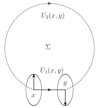
Figure 1: Local gauge transformation at two points $x$ and $y$. Two Wilson line between $x$ and $y$ are presented. The solid line is “short” Wilson line while the dashed line denotes the “longer” one. When $|x-y|\to 0$, the gauge transformation along $U_{1}(x,y)$ will be discontinuous.

In the present work we try to connect one-dimensional spinless fermionic system and bosonic system with discontinuous gauge transformation. We will show that free fermions can be mapped into bosons with a $\delta$-function type vector-potential, and vice versa, which reveal an interesting connection between boson-fermion duality and gauge symmetry. It is also possible to generalize the discussions on one-dimensional system to other space-time dimensions and symmetries.

We start with one-body problem in one dimensional quantum mechanics. Consider a charged scalar particle in a magnetic field. Its motion is governed by Schrödinger equation with gauge potential $A_{i}=(A_{0},A_{1})$

$$\left[-\frac{1}{2}\left(\partial_{x}+ieA_{1}\right)^{2}+V(x)\right]\phi(x,t)=i\left(\frac{\partial}{\partial t}+ieA_{0}\right)\phi(x,t),$$ (1)

For simplicity we adopt the system of natural units and take the particle mass $m=1$, $\phi(x,t)$ is the wave function, $e$ is the electric charge of the particle. It is well known that Eq.(1) is invariant under $U(1)$ gauge transformation

$$\phi(x,t)\to\phi^{\prime}(x,t) =\phi(x,t)e^{i\alpha(x,t)},$$ (2)

$$A_{i}(x,t)\to A^{\prime}_{i}(x,t) =A_{i}(x,t)-\frac{1}{e}\frac{\partial}{\partial x_{i}}\alpha(x,t),$$ (3)

where $i=0,~{}1$ corresponding to $t,~{}x$ respectively. As discussed above, the choice of the phase at one point should not be affected by another, so it is reasonable that the phase function $\alpha(x,t)$ can be discontinuous. Here we let $\alpha(x,t)=\pi\theta(x)$, where $\theta(x)$ is the Heaviside step function, $\alpha$ is independent of $t$. Then we have the discontinuous gauge transformation

$$\phi(x,t)\to\phi^{\prime}(x,t) =\phi(x,t)e^{i\pi\theta(x)},$$ (4)

$$A_{0}(x,t)\to A^{\prime}_{0}(x,t) =A_{0}(x,t),$$ (5)

$$A_{1}(x,t)\to A^{\prime}_{1}(x,t) =A_{1}(x,t)-\frac{\pi}{e}\delta(x),$$ (6)

$\delta(x)$ is the Dirac delta function. The transformation in Eq.(4) can be expressed as

$$\phi^{\prime}(x,t)=\left\{\begin{aligned} -&\phi(x,t),~{}~{}~{}~{}&x>0;\\ &\phi(x,t),~{}~{}~{}~{}&x<0.\end{aligned}\right.$$ (7)

Now we assume that $\phi(x,t)$ is an odd function of $x$, i.e., $\phi(-x,t)=-\phi(x,t)$, then for $\phi^{\prime}(x,t)$ we have $\phi^{\prime}(-x,t)=\phi^{\prime}(x,t)$, which means that $\phi^{\prime}(x,t)$ is an even function. So we have transform an odd wave function into an even wave function, at the cost of introducing a $\delta$-type potential in the gauge field. Even functions can also be transformed into odd functions under the same transformation.

Before further discussions we should make a few remarks on the vector potential. In fact there is no magnetic field $B$ in $1+1$ dimensions, even if it exists, charged particle will not couple to the magnetic field. Further more, it is a little tricky to talk about “vector potential”, because $A$ is actually a scalar in $1+1$ dimensions [19]. In our case, we just take $A$ as an auxiliary vector potential, also for the sake of simplicity, we will set $A_{i}=0$ and only keep the $\delta$ term in the following discussions for $1+1$ dimensions. $A$ will make sense in higher dimensions. With these assumptions, after the gauge transformation, the new field $\phi^{\prime}(x,t)$ then satisfies the Schrödinger equation

$$-\frac{1}{2}\Big{[}\partial_{x}-i\pi\delta(x)\Big{]}^{2}\phi^{\prime}(x,t)=i\frac{\partial}{\partial t}\phi^{\prime}(x,t).$$ (8)

To see how anti-symmetric wave function transform into symmetric more clearly, we consider a class of equations which approach to Eq.(8) when $\epsilon\to 0$. We restrained the system with an infinite square potential well, thus one can study the stationary state problem

$$-\frac{1}{2}\left[\left(\frac{\partial}{\partial x}-i\frac{\epsilon}{x^{2}+\epsilon^{2}}\right)^{2}+V(x)\right]\phi^{\prime}(x)=E_{n}\phi^{\prime}(x)$$ (9)

with

$$V(x)=\left\{\begin{aligned} &0,~{}~{}~{}~{}~{}~{}&|x|<a;\\ &\infty,~{}~{}~{}~{}~{}~{}&|x|>a,\end{aligned}\right.$$ (10)

where $E_{n}$ is the energy level. The eigenfunctions for different values of $\epsilon$ are shown in Fig.2. When $\epsilon$ is large, the anti-symmetric imaginary part is dominant. When $\epsilon$ takes small value the symmetric real part become important. When $\epsilon\to 0$, $\epsilon/(x^{2}+\epsilon^{2})\to\pi\delta(x)$, and the anti-symmetric imaginary part of wave function disappears, we finally arrive at a symmetric wave function.

Figure 2: The wave functions of Eq.(4) correspond to $n=2$ at $\epsilon=10$ (a), $\epsilon=1$ (b), $\epsilon=0.1$ (c) and $\epsilon=0.001$ (d). The solid lines denote the real parts while the dashed lines show the imaginary parts of the wave functions.

In [11][12], a fermionic system in an $\varepsilon(x;c)$ potential is proved to be equivalent with a bosonic system in $\delta(x;v)$ potential, with the coupling strength reversed, i.e., $v=1/c$, here $\varepsilon(x;c)\equiv\chi(x;-1,0,-1,-4c)$, and $\delta(x;v)\equiv\chi(x;-1,-v,-1,0)=v\delta(x)$. $\chi$ is defined by [12]

$$\chi(x;\alpha,\beta,\gamma,\delta)=\displaystyle{\lim_{a\to+0}}\left[\left(-\frac{1}{a}+\frac{\gamma-1}{\delta}\right)\delta(x+a)+\frac{1-\alpha\gamma}{\beta a^{2}}\delta(x)+\left(-\frac{1}{a}+\frac{\alpha-1}{\delta}\right)\delta(x-a)\right].$$ (11)

In fact what we have discussed above is an extreme case of such a strong-weak duality. To see this clearly, Eq.(8) can be reexpressed as a Schrödinger equation with a $\delta^{2}(x)$ potential

$$-\frac{1}{2}\frac{\partial^{2}}{\partial x^{2}}\phi^{\prime}(x,t)-\pi^{2}\delta^{2}(x)\phi^{\prime}(x,t)=i\frac{\partial}{\partial t}\phi^{\prime}(x,t),$$ (12)

because $\exp(i\pi\theta(x))=\exp(-i\pi\theta(x))$, the wave function satisfies the same equation when replacing $\pi$ with $-\pi$. When $c=a/2\to 0$, $\varepsilon(x;c)\to 0$, Schrödinger equation with $\varepsilon$ interaction then degenerates to a free particle equation; In another hand, $v=1/c\to\infty$, $v\delta(x)$ then becomes a $\delta$-interaction with infinite coupling strength, which can be regarded as a $\delta^{2}(x)$ interaction, because that when $x$ is close to $0$, $\delta^{2}(x)\sim\delta(0)\delta(x)$, which is a $\delta(x)$ interaction with an infinite coupling strength $\delta(0)$. Thus a fermionic system with zero coupling strength $\varepsilon$-interaction is equivalent to a bosonic system with infinite coupling strength $\delta$-interaction.

Now we turn to the two-particle system with a wave function $\Psi(x_{1},x_{2},t)$, $x_{i}(i=1,~{}2)$ is the coordinate of the $i$-th particle. Introducing the discontinuous gauge transformation

$$\Psi(x_{1},x_{2},t)\to\Psi^{\prime}(x_{1},x_{2},t)=\Psi(x_{1},x_{2},t)e^{i\pi\theta(x_{1}-x_{2})},$$ (13)

one can immediately get that

$$\Psi^{\prime}(x_{1},x_{2},t)=\left\{\begin{aligned} -&\Psi(x_{1},x_{2},t),~{}~{}~{}~{}~{}~{}&x_{1}>x_{2};\\ &\Psi(x_{1},x_{2},t),~{}~{}~{}~{}~{}~{}&x_{1}<x_{2}.\end{aligned}\right.$$ (14)

Notice that the sign before the $\delta$ function is opposite for the two particles. Now we assume that $\Psi(x_{1},x_{2},t)$ is anti-symmetric under the exchange of $x_{1}$ and $x_{2}$, i.e., a wave function for fermionic system, then $\Psi^{\prime}(x_{1},x_{2},t)$ should not change when exchanging $x_{1}$ and $x_{2}$, which is a wave function of bosons. Thus we have transformed a wave function of fermion into bosons under a discontinuous gauge transformation, at the cost of introducing a $\delta$-type interaction in the derivative of wave function. The two-body Schrödinger equation then reads

$$-\frac{1}{2}\left[\left(\frac{\partial}{\partial x_{1}}-i\pi\delta(x_{1}-x_{2})\right)^{2}+\left(\frac{\partial}{\partial x_{2}}+i\pi\delta(x_{1}-x_{2})\right)^{2}\right]\Psi^{\prime}(x_{1},x_{2},t)=i\frac{\partial}{\partial t}\Psi^{\prime}(x_{1},x_{2},t).$$ (15)

Similarly one can consider $n$-particle system, $x_{i}$ is the coordinate of the $i$-th particle. Then we perform the gauge transformation on the wave function $\Psi(x_{1},\cdots,x_{i},\cdots,x_{n})$:

$$\Psi(x_{1},\cdots,x_{i},\cdots,x_{n})\to\Psi^{\prime}(x_{1},\cdots,x_{n})=\Psi(x_{1},\cdots,x_{n})\exp{\left[i\pi\displaystyle{\sum_{1\leq i<j\leq n}\theta(x_{i}-x_{j})}\right]}.$$ (16)

One can examine that $\Psi^{\prime}$ will be multiplied by a $(-1)$ when exchanging the coordinates of any pair of particles. The wave function then satisfies the $n-$body Schrödinger equation

$$-\frac{1}{2}\displaystyle{\sum_{i=1}^{n}}\left[\frac{\partial}{\partial x_{i}}-i\pi\displaystyle{\sum_{\begin{subarray}{c}l,~{}k\\ 1\leq l<i<k\leq n\end{subarray}}}\left(\delta(x_{i}-x_{k})-\delta(x_{l}-x_{i})\right)\right]^{2}\Psi^{\prime}(x_{1},\cdots,x_{n})=i\frac{\partial}{\partial t}\Psi^{\prime}(x_{1},\cdots,x_{n}).$$ (17)

The $\delta$-function in the above equation can be understood as Pauli exclusion principle, which states that two or more identical fermions cannot occupy the same quantum state within a quantum system simultaneously. In one dimensional quantum mechanics, when the interaction term contains $V=\delta(x_{i}-x_{j})$, particles can not have the same coordinates at the same time, because that when $x_{i}=x_{j}$, $V$ will be infinite. In one dimensional system the quantum states are characterized by the space-time coordinates, so Pauli exclusion principle states that two fermions can not have the same coordinates at the same time, which indicates that there is a $\delta(x_{i}-x_{j})$ interaction in the equation of motion.

The above discussions on one dimensional system can also be generalized into other space-time dimensions. Now we will show that for an one-component scalar field with $U(1)$ symmetry, one can also build up boson-fermion duality in $2+1$ dimensions. Consider a gauge potential $\vec{A}=(-\frac{\pi}{2e}\delta(x),-\frac{\pi}{2e}\delta(y))$ and a symmetric wave function $\phi(\vec{r})$. For any $\vec{r}$ and $-\vec{r}$, one can link these two points with product of two Wilson lines $U_{L_{2}}(\vec{r},0)$ and $U_{L_{1}}(0,-\vec{r}\,)$:

$$U_{L_{2}}(\vec{r},0)U_{L_{1}}(0,-\vec{r}\,) =\exp\left(ie\int_{L_{1}}\vec{A}\cdot d\vec{l}\right)\exp\left(ie\int_{L_{2}}\vec{A}\cdot d\vec{l}\right)$$

$$=\exp\left\{-i\frac{\pi}{2}\int^{0}_{r}~{}dR\Big{[}\cos(\theta+\pi)~{}\delta\left(R\cos(\theta+\pi)\right)+\sin(\theta+\pi)~{}\delta\left(R\sin(\theta+\pi)\right)\Big{]}\right.$$

$$~{}~{}~{}~{}~{}~{}~{}~{}\,\,\,\,-i\left.\frac{\pi}{2}\int^{r}_{0}~{}dR\Big{[}\cos\theta~{}\delta(R\cos\theta)+\sin\theta~{}\delta(R\sin\theta)\Big{]}\right\}$$

$$=-1,$$ (18)

where $L_{1}$ is a straight line from $-\vec{r}$ to $0$ and $L_{2}$ is a straight line from $0$ to $\vec{r}$, $r$ and $\theta$ is the polar radius and angular respectively. If $\phi(\vec{r})$ is an odd function, then $\phi^{\prime}(\vec{r})$ will be an even function. Note that one can link $\vec{r}$ and $-\vec{r}$ by Wilson lines along other paths. However, every path links $\vec{r}$ and $-\vec{r}$ will pass $x$ and $y$ axes once. Every time passing through an axes will contribute a phase $\exp(i\pi/2)$, finally contributes a factor $(-1)$ to the relative phase of the two points.

In 2+1 dimensions we can also consider two components vector wave function under $U(1)\times U(1)$ symmetry. Consider a wave function $\Phi(\vec{r},t)=(\phi_{1}(\vec{r},t),~{}\phi_{2}(\vec{r},t))$, where $\vec{r}=(x,y)$. We perform the gauge transformation

$$\Phi(\vec{r},t)=(\phi_{1}(\vec{r},t),~{}\phi_{2}(\vec{r},t)) \to \Phi^{\prime}(\vec{r},t)=(e^{i\pi\theta(x)}\phi_{1}(\vec{r},t),~{}~{}e^{i\pi\theta(y)}\phi_{2}(\vec{r},t))$$ (19)

$$= \left\{\begin{aligned} &(-\phi_{1}(\vec{r},t),-\phi_{2}(\vec{r},t)),~{}~{}~{}~{}~{}~{}&x>0,~{}y>0;\\ &(\phi_{1}(\vec{r},t),-\phi_{2}(\vec{r},t)),~{}~{}~{}~{}~{}~{}&x<0,~{}y>0;\\ &(\phi_{1}(\vec{r},t),\phi_{2}(\vec{r},t)),~{}~{}~{}~{}~{}~{}&x<0,~{}y<0;\\ &(-\phi_{1}(\vec{r},t),\phi_{2}(\vec{r},t)),~{}~{}~{}~{}~{}~{}&x>0,~{}y<0.\end{aligned}\right.$$

If $\Phi(\vec{r},t)$ is an odd function with $\vec{r}$, i.e. $\Phi(-\vec{r},t)=\Phi(\vec{r},t)$, then $\Phi^{\prime}(-\vec{r},t)=-\Phi^{\prime}(\vec{r},t)$, which means that $\Phi^{\prime}(\vec{r},t)$ is an even function. Fig.3 shows that an odd vector wave function transforms into an even vector wave function under Eq.(19).

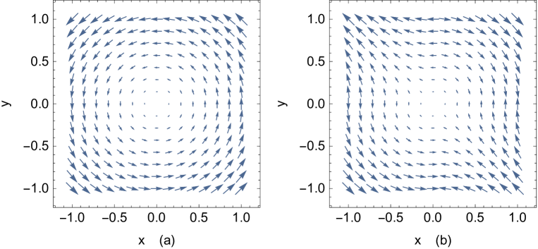
Figure 3: The gauge transformation Eq.(19). (a) shows an anti-symmetric vector wave function in 2 spatial dimensions. (b) is a symmetric vector wave function which is got by acting Eq.(19) on (a).

The gauge transformation on gauge potential $A_{i}$ then becomes

$${A}_{0}(\vec{r},t) \to A^{\prime}_{0}(\vec{r},t),$$ (20)

$${A}_{x}(\vec{r},t) \to{A}^{\prime}_{x}(\vec{r},t)={A}_{x}(\vec{r},t)-\frac{\pi}{e}\delta(x),$$ (21)

$${A}_{y}(\vec{r},t) \to{A}^{\prime}_{y}(\vec{r},t)={A}_{y}(\vec{r},t)-\frac{\pi}{e}\delta(y).$$ (22)

One can also construct many-body equations in 2+1 dimensions, just as what we have done for $1+1$ dimensional case. These discussions can also be generalized to higher space-time dimensions.

The Aharonov-Bohm effect [20] states that outside the region where magnetic field $B$ is confined, the vector potential may still causes observable effects. The above discussions also reveal some novel properties of vector potential. If the vector potential is confined in a $n-1$ dimensional hyperplane in $n$ spatial dimensions, it can also have physical effects. For certain configurations they may affect the shape of wave functions. In addition, this work only consider scalar wave functions governed by Schrödinger equation. Similar discussions can be performed to Dirac equations as well. Further more, in this work we only consider $U(1)$ and $U(1)\times U(1)$ groups. It should be also interesting of generalizing this work to non-Abelian symmetries. We leave these for a further research.

To summarize, we build up boson-fermion duality under the spirit of local gauge symmetry. The non-relativistic bosonic (fermionic) system can be mapped into a fermionic (bosonic) system with $\delta$-type gauge interactions. This duality may open a door to a deeper understanding of the relationship between exchange statistics and gauge symmetry.

Acknowledgments

We thank Dr. Jian-Ping Dai for valuable discussions.

References

- [1] M. Girardeau, J. Math. Phys. 1, 516 (1960).
- [2] M. Girardeau, Phys. Rev. B 139, 500 (1965).
- [3] D. C. Mattis and E. H. Lieb, J. Math. Phys. 6, 304 (1965).
- [4] S. R. Coleman, Phys. Rev. D 11, 2088 (1975).
- [5] S. Tomonaga, Prog. Theor. Phys. 5, 544 (1950).
- [6] J. M. Luttinger, J. Math. Phys. 4, 1154 (1963).
- [7] H. J. Schmidt, J. Schnack, Physica. A 260, 479 (1998).
- [8] M. Crescimanno and A. S. Landsberg, Phys. Rev. A 63, 035601 (2001).
- [9] Y. Freundlich, Nucl. Phys. B 36, 621 (1972).
- [10] P. C. W. Davies, J. Phys. A 11, 179 (1978).
- [11] T. Cheon and T. Shigehara, Phys. Lett. A 243, 111 (1998).
- [12] T. Cheon and T. Shigehara, Phys. Rev. Lett. 82, 2536 (1999).
- [13] B. Basu-Mallick and T. Bhattacharyya, Mod. Phys. Lett. A 25, 715 (2010).
- [14] H. Grosse, E. Langmann and C. Paufler, J. Phys. A 37, 4579 (2004)
- [15] T. Cheon, T. Fulop and I. Tsutsui, Annals Phys. 294, 1 (2001).
- [16] T. Fulop and I. Tsutsui, Phys. Lett. A 264, 366 (2000).
- [17] S. Ohya, J. Phys. Conf. Ser. 563, no. 1, 012021 (2014).
- [18] T. Nagasawa, M. Sakamoto and K. Takenaga, Phys. Lett. B 562, 358 (2003).
- [19] H. J. W. Muller-Kirsten, Electrodynamics: An Introduction Including Quantum Effects, World Scientific, 2004.
- [20] Y. Aharonov and D. Bohm, Phys. Rev. 115, 485 (1959).