Total Variation Denoising via the Moreau Envelope

Abstract

Total variation denoising is a nonlinear filtering method well suited for the estimation of piecewise-constant signals observed in additive white Gaussian noise. The method is defined by the minimization of a particular non-differentiable convex cost function. This paper describes a generalization of this cost function that can yield more accurate estimation of piecewise constant signals. The new cost function involves a non-convex penalty (regularizer) designed to maintain the convexity of the cost function. The new penalty is based on the Moreau envelope. The proposed total variation denoising method can be implemented using forward-backward splitting.

I Introduction

Total variation (TV) denoising is a nonlinear filtering method based on the assumption that the underlying signal is piecewise constant (equivalently, the derivative of the underlying signal is sparse) [45]. Such signals arise in geoscience, biophysics, and other areas [31]. The TV denoising technique is also used in conjunction with other methods in order to process more general types of signals [26, 24, 23, 20].

Total variation denoising is prototypical of methods based on sparse signal models. It is defined by the minimization of a convex cost function comprising a quadratic data fidelity term and a non-differentiable convex penalty term. The penalty term is the composition of a linear operator and the $\ell_{1}$ norm. Although the $\ell_{1}$ norm stands out as the convex penalty that most effectively induces sparsity [27], non-convex penalties can lead to more accurate estimation of the underlying signal [37, 38, 40, 44, 50].

A few recent papers consider the prescription of non-convex penalties that maintain the convexity of the TV denoising cost function [30, 32, 48, 1]. (The motivation for this is to leverage the benefits of both non-convex penalization and convex optimization, e.g., to accurately estimate the amplitude of jump discontinuities while guaranteeing the uniqueness of the solution.) The penalties considered in these works are separable (additive). But non-separable penalties can outperform separable penalties in this context. This is because preserving the convexity of the cost function is a severely limiting requirement. Non-separable penalties can more successfully meet this requirement because they are more general than separable penalties [47].

This paper proposes a non-separable non-convex penalty for total variation denoising that generalizes the standard penalty and maintains the convexity of the cost function to be minimized. The new penalty, which is based on the Moreau envelope, can more accurately estimate the amplitudes of jump discontinuities in an underlying piecewise constant signal.

I-A Relation to Prior Work

Numerous non-convex penalties and algorithms have been proposed to outperform $\ell_{1}$-norm regularization for the estimation of sparse signals e.g., [10, 8, 39, 34, 33, 12, 15, 43, 53, 13, 51]. However, few of these methods maintain the convexity of the cost function. The prescription of non-convex penalties maintaining cost function convexity was pioneered by Blake, Zisserman, and Nikolova [6, 36, 40, 39], and further developed in Refs. [3, 4, 14, 20, 28, 30, 32, 42, 46, 48]. These works rely on the presence of both strongly and weakly convex terms, which is also exploited in [35].

The proposed penalty is expressed as a differentiable convex function subtracted from the standard penalty (i.e., $\ell_{1}$ norm). Previous works also use this idea [41, 47, 42]. But the differentiable convex functions used therein are either separable [41, 42] or sums of bivariate functions [47].

In parallel with the submission of this paper, Carlsson has also proposed using Moreau envelopes to prescribe non-trivial convex cost functions [9]. While the approach in [9] starts with a given non-convex cost function (e.g., with the $\ell_{0}$ pseudo-norm penalty) and seeks the convex envelope, our approach starts with the $\ell_{1}$-norm penalty and seeks a class of convexity-preserving penalties.

Some forms of generalized TV are based on infimal convolution (related to the Moreau envelope) [49, 11, 7, 5]. But these works propose convex penalties suitable for non-piecewise-constant signals, while we propose non-convex penalties suitable for piecewise-constant signals.

II Total Variation Denoising

Definition 1.

Given $y\in\mathbb{R}^{N}$ and ${\lambda}>0$, total variation denoising is defined as

$$\operatorname{tvd}(y;{\lambda}) =\arg\min_{x\in\mathbb{R}^{N}}\bigl{\{}\tfrac{1}{2}\lVert y-x\rVert_{2}^{2}+{\lambda}\lVert Dx\rVert_{1}\bigr{\}}$$ (1)

$$=\operatorname{prox}_{{\lambda}\lVert D\,\cdot\,\rVert_{1}}(y)$$ (2)

where $D$ is the $(N-1)\times N$ matrix

$$D=\begin{bmatrix}-1&1&&&\\ &-1&1&&\\ &&\ddots&\ddots&\\ &&&-1&1\end{bmatrix}.$$ (3)

As indicated in (2), TV denoising is the proximity operator [16] of the function $x\mapsto{\lambda}\lVert Dx\rVert_{1}$. It is convenient that TV denoising can be calculated exactly in finite-time [17, 22, 29, 18].

III Moreau Envelope

Before we define the non-differentiable non-convex penalty in Sec. IV, we first define a differentiable convex function. We use the Moreau envelope from convex analysis [2].

Definition 2.

Let $\alpha\geqslant 0$. We define $S_{\alpha}\colon\mathbb{R}^{N}\to\mathbb{R}$ as

$$S_{\alpha}(x)=\min_{v\in\mathbb{R}^{N}}\bigl{\{}\lVert Dv\rVert_{1}+\tfrac{\alpha}{2}\lVert x-v\rVert_{2}^{2}\,\bigr{\}}$$ (4)

where $D$ is the first-order difference matrix (3).

If $\alpha>0$, then $S_{\alpha}$ is the Moreau envelope of index $\alpha^{-1}$ of the function $x\mapsto\lVert Dx\rVert_{1}$.

Proposition 1.

The function $S_{\alpha}$ can be calculated by

$$S_{0}(x) =0$$ (5)

$$S_{\alpha}(x) =\lVert D\operatorname{tvd}(x;1/\alpha)\rVert_{1}$$

$$\hskip 30.00005pt{}+\tfrac{\alpha}{2}\lVert x-\operatorname{tvd}(x;1/\alpha)\rVert_{2}^{2},\quad\alpha>0.$$ (6)

Proof.

For $\alpha=0$: Setting $\alpha=0$ and $v=0$ in (4) gives (5). For $\alpha>0$: By the definition of TV denoising, the $v\in\mathbb{R}^{N}$ minimizing the function in (4) is the TV denoising of $x$, i.e., $v^{\mathsf{opt}}=\operatorname{tvd}(x,1/\alpha)$. ∎

Proposition 2.

Let $\alpha\geqslant 0$. The function $S_{\alpha}$ satisfies

$$0\leqslant S_{\alpha}(x)\leqslant\lVert Dx\rVert_{1},\ \ \forall x\in\mathbb{R}^{N}.$$ (7)

Proof.

From (4), we have $S_{\alpha}(x)\leqslant\lVert Dv\rVert_{1}+(\alpha/2)\lVert x-v\rVert_{2}^{2}$ for all $v\in\mathbb{R}^{N}$. In particular, $v=x$ leads to $S_{\alpha}(x)\leqslant\lVert Dx\rVert_{1}$. Also, $S_{\alpha}(x)\geqslant 0$ since $S_{\alpha}(x)$ is defined as the minimum of a non-negative function. ∎

Proposition 3.

Let $\alpha\geqslant 0$. The function $S_{\alpha}$ is convex and differentiable.

Proof.

It follows from Proposition 12.15 in Ref. [2]. ∎

Proposition 4.

Let $\alpha\geqslant 0$. The gradient of $S_{\alpha}$ is given by

$$\nabla S_{0}(x) =0$$ (8)

$$\nabla S_{\alpha}(x) =\alpha\bigl{(}x-\operatorname{tvd}(x;1/\alpha)\bigr{)},\quad\alpha>0$$ (9)

where $\operatorname{tvd}$ denotes total variation denoising (1).

Proof.

Since $S_{\alpha}$ is the Moreau envelope of index $\alpha^{-1}$ of the function $x\mapsto\lVert Dx\rVert_{1}$ when $\alpha>0$, it follows by Proposition 12.29 in Ref. [2] that

$$\nabla S_{\alpha}(x)=\alpha\bigl{(}x-\operatorname{prox}_{(1/\alpha)\lVert D\,\cdot\,\rVert_{1}}(x)\bigr{)}.$$ (10)

This proximity operator is TV denoising, giving (9). ∎

IV Non-convex Penalty

To strongly induce sparsity of $Dx$, we define a non-convex generalization of the standard TV penalty. The new penalty is defined by subtracting a differentiable convex function from the standard penalty.

Definition 3.

Let $\alpha\geqslant 0$. We define the penalty $\psi_{\alpha}\colon\mathbb{R}^{N}\to\mathbb{R}$ as

$$\psi_{\alpha}(x)=\lVert Dx\rVert_{1}-S_{\alpha}(x)$$ (11)

where $D$ is the matrix (3) and $S_{\alpha}$ is defined by (4).

The proposed penalty is upper bounded by the standard TV penalty, which is recovered as a special case.

Proposition 5.

Let $\alpha\geqslant 0$. The penalty $\psi_{\alpha}$ satisfies

$$\psi_{0}(x)=\lVert Dx\rVert_{1},\ \ \forall x\in\mathbb{R}^{N}$$ (12)

and

$$0\leqslant\psi_{\alpha}(x)\leqslant\lVert Dx\rVert_{1},\ \ \forall x\in\mathbb{R}^{N}.$$ (13)

Proof.

It follows from (5) and (7). ∎

When a convex function is subtracted from another convex function [as in (11)], the resulting function may well be negative on part of its domain. Inequality (13) states that the proposed penalty $\psi_{\alpha}$ avoids this fate. This is relevant because the penalty function should be non-negative.

Figures in the supplemental material show examples of the proposed penalty $\psi_{\alpha}$ and the function $S_{\alpha}$.

V Enhanced TV Denoising

We define ‘Moreau-enhanced’ TV denoising. If $\alpha>0$, then the proposed penalty penalizes large amplitude values of $Dx$ less than the $\ell_{1}$ norm does (i.e., $\psi_{\alpha}(x)\leqslant\lVert Dx\rVert_{1}$), hence it is less likely to underestimate jump discontinuities.

Definition 4.

Given $y\in\mathbb{R}^{N}$, ${\lambda}>0$, and $\alpha\geqslant 0$, we define Moreau-enhanced total variation denoising as

$$\operatorname{mtvd}(y;{\lambda},\alpha)=\arg\min_{x\in\mathbb{R}^{N}}\bigl{\{}\tfrac{1}{2}\lVert y-x\rVert_{2}^{2}+{\lambda}\psi_{\alpha}(x)\bigr{\}}$$ (14)

where $\psi_{\alpha}$ is given by (11).

The parameter $\alpha$ controls the non-convexity of the penalty. If $\alpha=0$, then the penalty is convex and Moreau-enhanced TV denoising reduces to TV denoising. Greater values of $\alpha$ make the penalty more non-convex. What is the greatest value of $\alpha$ that maintains convexity of the cost function? The critical value is given by Theorem 1.

Theorem 1.

Let ${\lambda}>0$ and $\alpha\geqslant 0$. Define $F_{\alpha}\colon\mathbb{R}^{N}\to\mathbb{R}$ as

$$F_{\alpha}(x)=\tfrac{1}{2}\lVert y-x\rVert_{2}^{2}+{\lambda}\psi_{\alpha}(x)$$ (15)

where $\psi_{\alpha}$ is given by (11). If

$$0\leqslant\alpha\leqslant 1/{\lambda}$$ (16)

then $F_{\alpha}$ is convex. If $0\leqslant\alpha<1/{\lambda}$ then $F_{\alpha}$ is strongly convex.

Proof.

We write the cost function as

$$F_{\alpha}(x) =\tfrac{1}{2}\lVert y-x\rVert_{2}^{2}+{\lambda}\lVert Dx\rVert_{1}-{\lambda}S_{\alpha}(x)$$ (17)

$$=\tfrac{1}{2}\lVert y-x\rVert_{2}^{2}+{\lambda}\lVert Dx\rVert_{1}$$

$$\hskip 30.00005pt{}-{\lambda}\min_{v\in\mathbb{R}^{N}}\bigl{\{}\lVert Dv\rVert_{1}+\tfrac{\alpha}{2}\lVert x-v\rVert_{2}^{2}\,\bigr{\}}$$ (18)

$$=\max_{v\in\mathbb{R}^{N}}\bigl{\{}\tfrac{1}{2}\lVert y-x\rVert_{2}^{2}+{\lambda}\lVert Dx\rVert_{1}$$

$$\hskip 60.00009pt{}-{\lambda}\lVert Dv\rVert_{1}-\tfrac{{\lambda}\alpha}{2}\lVert x-v\rVert_{2}^{2}\,\bigr{\}}$$ (19)

$$=\max_{v\in\mathbb{R}^{N}}\bigl{\{}\tfrac{1}{2}(1-{\lambda}\alpha)\lVert x\rVert_{2}^{2}+{\lambda}\lVert Dx\rVert_{1}+g(x,v)\,\bigr{\}}$$ (20)

$$=\tfrac{1}{2}(1-{\lambda}\alpha)\lVert x\rVert_{2}^{2}+{\lambda}\lVert Dx\rVert_{1}+\max_{v\in\mathbb{R}^{N}}g(x,v)$$ (21)

where $g(x,v)$ is affine in $x$. The last term is convex as it is the point-wise maximum of a set of convex functions. Hence, $F_{\alpha}$ is a convex function if $1-{\lambda}\alpha\geqslant 0$. If $1-{\lambda}\alpha>0$, then $F_{\alpha}$ is strongly convex (and strictly convex). ∎

VI Algorithm

Proposition 6.

Let $y\in\mathbb{R}^{N}$, ${\lambda}>0$, and $0<\alpha<1/{\lambda}$. Then $x^{(k)}$ produced by the iteration

$$z^{(k)} =y+{\lambda}\alpha\bigl{(}x^{(k)}-\operatorname{tvd}(x^{(k)};1/\alpha)\bigr{)}$$ (22a)

$$x^{(k+1)} =\operatorname{tvd}(z^{(k)};{\lambda}).$$ (22b)

converges to the solution of the Moreau-enhanced TV denoising problem (14).

Proof.

If the cost function (15) is strongly convex, then the minimizer can be calculated using the forward-backward splitting (FBS) algorithm [2, 16]. This algorithm minimizes a function of the form

$$F(x)=f_{1}(x)+f_{2}(x)$$ (23)

where both $f_{1}$ and $f_{2}$ are convex and $\nabla f_{1}$ is additionally Lipschitz continuous. The FBS algorithm is given by

$$z^{(k)} =x^{(k)}-\mu\bigl{[}\nabla f_{1}(x^{(k)})\bigr{]}$$ (24a)

$$x^{(k+1)} =\arg\min_{x}\big{\{}\tfrac{1}{2}\lVert z^{(k)}-x\rVert_{2}^{2}+\mu f_{2}(x)\big{\}}$$ (24b)

where $0<\mu<2/\rho$ and $\rho$ is the Lipschitz constant of $\nabla f_{1}$. The iterates $x^{(k)}$ converge to a minimizer of $F$.

To apply the FBS algorithm to the proposed cost function (15), we write it as

$$F_{\alpha}(x) =\tfrac{1}{2}\lVert y-x\rVert_{2}^{2}+{\lambda}\psi_{\alpha}(x),$$ (25)

$$=\tfrac{1}{2}\lVert y-x\rVert_{2}^{2}+{\lambda}\lVert Dx\rVert_{1}-{\lambda}S_{\alpha}(x)$$ (26)

$$=f_{1}(x)+f_{2}(x)$$ (27)

where

$$f_{1}(x) =\tfrac{1}{2}\lVert y-x\rVert_{2}^{2}-{\lambda}S_{\alpha}(x)$$ (28a)

$$f_{2}(x) ={\lambda}\lVert Dx\rVert_{1}.$$ (28b)

The gradient of $f_{1}$ is given by

$$\nabla f_{1}(x) =x-y-{\lambda}\nabla S_{\alpha}(x)$$ (29)

$$=x-y-{\lambda}\alpha\bigl{(}x-\operatorname{tvd}(x;1/\alpha)\bigr{)}$$ (30)

using Proposition 4. Subtracting $S_{\alpha}$ from $f_{1}$ does not increase the Lipschitz constant of $\nabla f_{1}$, the value of which is 1. Hence, we may set $0<\mu<2$.

Using (28), the FBS algorithm (24) becomes

$$z^{(k)} =x^{(k)}-\mu\bigl{[}x^{(k)}-y$$

$$\hskip 40.00006pt{}-{\lambda}\alpha\bigl{(}x^{(k)}-\operatorname{tvd}(x^{(k)};1/\alpha)\bigr{)}\bigr{]}$$ (31a)

$$x^{(k+1)} =\arg\min_{x}\big{\{}\tfrac{1}{2}\lVert z^{(k)}-x\rVert_{2}^{2}+\mu{\lambda}\lVert Dx\rVert_{1}\big{\}}.$$ (31b)

Note that (31b) is TV denoising (1). Using the value $\mu=1$ gives iteration (22). (Experimentally, we found this value yields fast convergence.) ∎

Each iteration of (22) entails solving two standard TV denoising problems. In this work, we calculate TV denoising using the fast exact C language program by Condat [17]. Like the iterative shrinkage/thresholding algorithm (ISTA) [19, 25], algorithm (22) can be accelerated in various ways.

We suggest not setting $\alpha$ too close to the critical value $1/{\lambda}$ because the FBS algorithm generally converges faster when the cost function is more strongly convex ($\alpha<1$).

In summary, the proposed Moreau-enhanced TV denoising method comprises the steps:

1. Set the regularization parameter ${\lambda}$ (${\lambda}>0$).

2. Set the non-convexity parameter $\alpha$ ($0\leqslant\alpha<1/{\lambda}$).

3. Initialize $x^{(0)}=0$.

4. Run iteration (22) until convergence.

VII Optimality Condition

To avoid terminating the iterative algorithm too early, it is useful to verify convergence using an optimality condition.

Proposition 7.

Let $y\in\mathbb{R}^{N}$, ${\lambda}>0$, and $0<\alpha<1/{\lambda}$. If $x$ is a solution to (14), then

$$\bigl{[}C\bigl{(}(x-y)/{\lambda}+\alpha(\operatorname{tvd}(x;1/\alpha)-x)\bigr{)}\bigr{]}_{n}\in\operatorname{sign}([Dx]_{n})$$ (32)

for $n=0,\dots,N-1$, where $C\in\mathbb{R}^{(N-1)\times N}$ is given by

$$C_{m,n}=\begin{cases}1,\ &m\geqslant n\\ 0,&m<n,\end{cases}\quad\text{i.e.,}\quad[Cx]_{n}=\sum_{m\leqslant n}x_{m}$$ (33)

and $\operatorname{sign}$ is the set-valued signum function

$$\operatorname{sign}(t)=\begin{cases}\{-1\},\ \ &t<0\\ [-1,1],&t=0\\ \{1\},&t>0.\end{cases}$$ (34)

According to (32), if $x\in\mathbb{R}^{N}$ is a minimizer, then the points $([Dx]_{n},u_{n})\in\mathbb{R}^{2}$ must lie on the graph of the signum function, where $u_{n}$ denotes the value on the left-hand side of (32). Hence, the optimality condition can be depicted as a scatter plot. Figures in the supplemental material show how the points in the scatter plot converge to the signum function as the algorithm (22) progresses.

Proof of Proposition 7.

A vector $x$ minimizes a convex function $F$ if $0\in\partial F(x)$ where $\partial F(x)$ is the subdifferential of $F$ at $x$. The subdifferential of the cost function (15) is given by

$$\partial F_{\alpha}(x)=x-y-{\lambda}\nabla S_{\alpha}(x)+\partial({\lambda}\lVert D\,\cdot\,\rVert_{1})(x)$$ (35)

which can be written as

$$\partial F_{\alpha}(x)=\{x-y-{\lambda}\nabla S_{\alpha}(x)+{\lambda}D^{\mathsf{T}}\!u\\ {}:u_{n}\in\operatorname{sign}([Dx]_{n}),\,u\in\mathbb{R}^{N-1}\}.$$ (36)

Hence, the condition $0\in\partial F_{\alpha}(x)$ can be written as

$$(y-x)/{\lambda}+\nabla S_{\alpha}(x)\\ {}\in\{D^{\mathsf{T}}\!u:u_{n}\in\operatorname{sign}([Dx]_{n}),\,u\in\mathbb{R}^{N-1}\}.$$ (37)

Let $C$ be a matrix of size $(N-1)\times N$ such that $CD^{\mathsf{T}}=-I$, e.g., (33). It follows that the condition $0\in\partial F_{\alpha}(x)$ implies that

$$\bigl{[}C\bigl{(}(x-y)/{\lambda}-\nabla S_{\alpha}(x)\bigr{)}\bigr{]}_{n}\in\operatorname{sign}([Dx]_{n})$$ (38)

for $n=0,\dots,N-1$. Using Proposition 4 gives (32). ∎

VIII Example

Figure 1: Total variation denoising using three different penalties. (The dashed line is the true noise-free signal.)

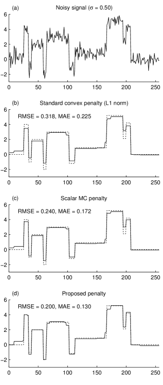
This example applies TV denoising to the noisy piecewise constant signal shown in Fig. 1(a). This is the ‘blocks’ signal (length $N=256$) generated by the Wavelab [21] function MakeSignal with additive white Gaussian noise ($\sigma=0.5$). We set the regularization parameter to ${\lambda}=\sqrt{N}\sigma/4$ following a discussion in Ref. [22]. For Moreau-enhanced TV denoising, we set the non-convexity parameter to $\alpha=0.7/{\lambda}$.

Figure 1 shows the result of TV denoising with three different penalties. In each case, a convex cost function is minimized. Figure 1(b) shows the result using standard TV denoising (i.e., using the $\ell_{1}$-norm). This denoised signal consistently underestimates the amplitudes of jump discontinuities, especially those occurring near other jump discontinuities of opposite sign. Figure 1(c) shows the result using a separable non-convex penalty [48]. This method can use any non-convex scalar penalty satisfying a prescribed set of properties. Here we use the minimax-concave (MC) penalty [52, 3] with non-convexity parameter set to maintain cost function convexity. This result significantly improves the root-mean-square error (RMSE) and mean-absolute-deviation (MAE), but still underestimates the amplitudes of jump discontinuities.

Moreau-enhanced TV denoising, shown in Fig. 1(d), further reduces the RMSE and MAE and more accurately estimates the amplitudes of jump discontinuities. The proposed non-separable non-convex penalty avoids the consistent underestimation of discontinuities seen in Figs. 1(b) and 1(c).

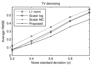
To further compare the denoising capability of the considered penalties, we calculate the average RMSE as a function of the noise level. We let the noise standard deviation span the interval $0.2\leqslant\sigma\leqslant 1.0$. For each $\sigma$ value, we calculate the average RMSE of 100 noise realizations. Figure 2 shows that the proposed penalty yields the lowest average RMSE for all $\sigma\geqslant 0.4$. However, at low noise levels, separable convexity-preserving penalties [48] perform better than the proposed non-separable convexity-preserving penalty.

Figure 2: TV denoising using four penalties: RMSE as a function of noise level.

IX Conclusion

This paper demonstrates the use of the Moreau envelope to define a non-separable non-convex TV denoising penalty that maintains the convexity of the TV denoising cost function. The basic idea is to subtract from a convex penalty its Moreau envelope. This idea should also be useful for other problems, e.g., analysis tight-frame denoising [41].

Separable convexity-preserving penalties [48] outperformed the proposed one at low noise levels in the example. It is yet to be determined if a more general class of convexity-preserving penalties can outperform both across all noise levels.

X Supplemental Figures

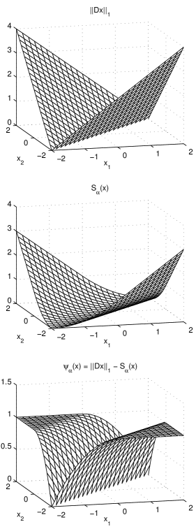
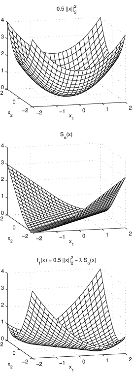
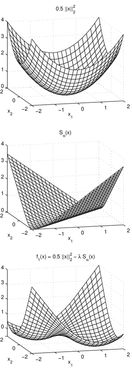
To gain intuition about the proposed penalty function and how it induces sparsity of $Dx$ while maintaining convexity of the cost function, a few illustrations are useful.

Figure 3 illustrates the proposed penalty, its sparsity-inducing behavior, and its relationship to the differentiable convex function $S_{\alpha}$. Figure 4 illustrates how the proposed penalty is able to maintain the convexity of the cost function.

Figure 3 shows the proposed penalty $\psi_{\alpha}$ defined in (11) for $\alpha=1$ and $N=2$. It can be seen that the penalty approximates the standard TV penalty $\lVert D\,\cdot\,\rVert_{1}$ for signals $x$ for which $Dx$ is approximately zero. But it increases more slowly than the standard TV penalty as $\lVert Dx\rVert\to\infty$. In that sense, it penalizes large values less than the standard TV penalty.

As shown in Fig. 3, the proposed penalty is expressed as the standard TV penalty minus the differentiable convex non-negative function $S_{\alpha}$. Since $S_{\alpha}$ is flat around the null space of $D$, the penalty $\psi_{\alpha}$ approximates the standard TV penalty around the null space of $D$. In addition, since $S_{\alpha}$ is non-negative, the penalty $\psi_{\alpha}$ lies below the standard TV penalty.

Figure 4 shows the differentiable part of the cost function $F_{\alpha}$ for $\alpha=1$, ${\lambda}=1$, and $N=2$. The differentiable part is given by $f_{1}$ in (28a). The total cost function is obtained by adding the standard TV penalty to $f_{1}$, see (23). Hence, $F_{\alpha}$ is convex if the differentiable part $f_{1}$ is convex. As can be seen in Fig. 4, the function $f_{1}$ is convex. We note that the function $f_{1}$ in this figure is not strongly convex. This is because we have used $\alpha=1/{\lambda}$. If $\alpha<1/{\lambda}$, then the function $f_{1}$ will be strongly convex (and hence $F_{\alpha}$ will also be strongly convex and have a unique minimizer). We recommend $\alpha<1/{\lambda}$.

Figure 5 shows the differentiable part $f_{1}$ of the cost function $F_{\alpha}$ for $\alpha=2$, ${\lambda}=1$, and $N=2$. Here, the function $f_{1}$ is non-convex because $\alpha>1/{\lambda}$ which violates the convexity condition.

In order to simplify the illustration, we have set $y=0$ in Fig. 4. In practice $y\neq 0$. But the only difference between the cases $y=0$ and $y\neq 0$ is an additive affine function which does not alter the convexity properties of the function.

In practice we are interested in the case $N\gg 2$, i.e., signals much longer than two samples. However, in order to illustrate the functions, we are limited to the case of $N=2$. We note that the case of $N=2$ does not fully illustrate the behavior of the proposed penalty. In particular, when $N=2$ the penalty is simply a linear transformation of a scalar function, which does not convey the non-separable behavior of the penalty for $N>2$.

A separate document has additional supplemental figures illustrating the convergence of the iterative algorithm (22). These figures show the optimality condition as a scatter plot. The points in the scatter plot converge to the signum function as the algorithm converges.

Figure 3: Penalty $\psi_{\alpha}$ with $\alpha=1$ for $N=2$.

Figure 4: Differentiable part $f_{1}$ of cost function with ${\lambda}=1$, $\alpha=1$ for $N=2$. The function is convex as $\alpha\leqslant 1/{\lambda}$.

Figure 5: Differentiable part $f_{1}$ of cost function with ${\lambda}=1$, $\alpha=2$ for $N=2$. The function is non-convex as $\alpha>1/{\lambda}$.

References

- [1] F. Astrom and C. Schnorr. On coupled regularization for non-convex variational image enhancement. In IAPR Asian Conf. on Pattern Recognition (ACPR), pages 786–790, November 2015.
- [2] H. H. Bauschke and P. L. Combettes. Convex Analysis and Monotone Operator Theory in Hilbert Spaces. Springer, 2011.
- [3] İ. Bayram. Penalty functions derived from monotone mappings. IEEE Signal Processing Letters, 22(3):265–269, March 2015.
- [4] I. Bayram. On the convergence of the iterative shrinkage/thresholding algorithm with a weakly convex penalty. IEEE Trans. Signal Process., 64(6):1597–1608, March 2016.
- [5] S. Becker and P. L. Combettes. An algorithm for splitting parallel sums of linearly composed monotone operators, with applications to signal recovery. J. Nonlinear and Convex Analysis, 15(1):137–159, 2014.
- [6] A. Blake and A. Zisserman. Visual Reconstruction. MIT Press, 1987.
- [7] M. Burger, K. Papafitsoros, E. Papoutsellis, and C.-B. Schönlieb. Infimal convolution regularisation functionals of BV and Lp spaces. J. Math. Imaging and Vision, 55(3):343–369, 2016.
- [8] E. J. Candès, M. B. Wakin, and S. Boyd. Enhancing sparsity by reweighted l1 minimization. J. Fourier Anal. Appl., 14(5):877–905, December 2008.
- [9] M. Carlsson. On convexification/optimization of functionals including an l2-misfit term. https://arxiv.org/abs/1609.09378, September 2016.
- [10] M. Castella and J.-C. Pesquet. Optimization of a Geman-McClure like criterion for sparse signal deconvolution. In IEEE Int. Workshop Comput. Adv. Multi-Sensor Adaptive Proc., pages 309–312, December 2015.
- [11] A. Chambolle and P.-L. Lions. Image recovery via total variation minimization and related problems. Numerische Mathematik, 76:167–188, 1997.
- [12] R. Chartrand. Shrinkage mappings and their induced penalty functions. In Proc. IEEE Int. Conf. Acoust., Speech, Signal Processing (ICASSP), pages 1026–1029, May 2014.
- [13] L. Chen and Y. Gu. The convergence guarantees of a non-convex approach for sparse recovery. IEEE Trans. Signal Process., 62(15):3754–3767, August 2014.
- [14] P.-Y. Chen and I. W. Selesnick. Group-sparse signal denoising: Non-convex regularization, convex optimization. IEEE Trans. Signal Process., 62(13):3464–3478, July 2014.
- [15] E. Chouzenoux, A. Jezierska, J. Pesquet, and H. Talbot. A majorize-minimize subspace approach for image regularization. SIAM J. Imag. Sci., 6(1):563–591, 2013.
- [16] P. L. Combettes and J.-C. Pesquet. Proximal splitting methods in signal processing. In H. H. Bauschke et al., editors, Fixed-Point Algorithms for Inverse Problems in Science and Engineering, pages 185–212. Springer-Verlag, 2011.
- [17] L. Condat. A direct algorithm for 1-D total variation denoising. IEEE Signal Processing Letters, 20(11):1054–1057, November 2013.
- [18] J. Darbon and M. Sigelle. Image restoration with discrete constrained total variation Part I: Fast and exact optimization. J. Math. Imaging and Vision, 26(3):261–276, 2006.
- [19] I. Daubechies, M. Defrise, and C. De Mol. An iterative thresholding algorithm for linear inverse problems with a sparsity constraint. Commun. Pure Appl. Math, 57(11):1413–1457, 2004.
- [20] Y. Ding and I. W. Selesnick. Artifact-free wavelet denoising: Non-convex sparse regularization, convex optimization. IEEE Signal Processing Letters, 22(9):1364–1368, September 2015.
- [21] D. Donoho, A. Maleki, and M. Shahram. Wavelab 850, 2005. http://www-stat.stanford.edu/%7Ewavelab/.
- [22] L. Dümbgen and A. Kovac. Extensions of smoothing via taut strings. Electron. J. Statist., 3:41–75, 2009.
- [23] S. Durand and J. Froment. Reconstruction of wavelet coefficients using total variation minimization. SIAM J. Sci. Comput., 24(5):1754–1767, 2003.
- [24] G. R. Easley, D. Labate, and F. Colonna. Shearlet-based total variation diffusion for denoising. IEEE Trans. Image Process., 18(2):260–268, February 2009.
- [25] M. Figueiredo and R. Nowak. An EM algorithm for wavelet-based image restoration. IEEE Trans. Image Process., 12(8):906–916, August 2003.
- [26] A. Gholami and S. M. Hosseini. A balanced combination of Tikhonov and total variation regularizations for reconstruction of piecewise-smooth signals. Signal Processing, 93(7):1945–1960, 2013.
- [27] T. Hastie, R. Tibshirani, and M. Wainwright. Statistical learning with sparsity: the lasso and generalizations. CRC Press, 2015.
- [28] W. He, Y. Ding, Y. Zi, and I. W. Selesnick. Sparsity-based algorithm for detecting faults in rotating machines. Mechanical Systems and Signal Processing, 72-73:46–64, May 2016.
- [29] N. A. Johnson. A dynamic programming algorithm for the fused lasso and -segmentation. J. Computat. Graph. Stat., 22(2):246–260, 2013.
- [30] A. Lanza, S. Morigi, and F. Sgallari. Convex image denoising via non-convex regularization with parameter selection. J. Math. Imaging and Vision, pages 1–26, 2016.
- [31] M. A. Little and N. S. Jones. Generalized methods and solvers for noise removal from piecewise constant signals: Part I – background theory. Proc. R. Soc. A, 467:3088–3114, 2011.
- [32] M. Malek-Mohammadi, C. R. Rojas, and B. Wahlberg. A class of nonconvex penalties preserving overall convexity in optimization-based mean filtering. IEEE Trans. Signal Process., 64(24):6650–6664, December 2016.
- [33] Y. Marnissi, A. Benazza-Benyahia, E. Chouzenoux, and J.-C. Pesquet. Generalized multivariate exponential power prior for wavelet-based multichannel image restoration. In Proc. IEEE Int. Conf. Image Processing (ICIP), pages 2402–2406, September 2013.
- [34] H. Mohimani, M. Babaie-Zadeh, and C. Jutten. A fast approach for overcomplete sparse decomposition based on smoothed l0 norm. IEEE Trans. Signal Process., 57(1):289–301, January 2009.
- [35] T. Möllenhoff, E. Strekalovskiy, M. Moeller, and D. Cremers. The primal-dual hybrid gradient method for semiconvex splittings. SIAM J. Imag. Sci., 8(2):827–857, 2015.
- [36] M. Nikolova. Estimation of binary images by minimizing convex criteria. In Proc. IEEE Int. Conf. Image Processing (ICIP), pages 108–112 vol. 2, 1998.
- [37] M. Nikolova. Local strong homogeneity of a regularized estimator. SIAM J. Appl. Math., 61(2):633–658, 2000.
- [38] M. Nikolova. Analysis of the recovery of edges in images and signals by minimizing nonconvex regularized least-squares. Multiscale Model. Simul., 4(3):960–991, 2005.
- [39] M. Nikolova. Energy minimization methods. In O. Scherzer, editor, Handbook of Mathematical Methods in Imaging, chapter 5, pages 138–186. Springer, 2011.
- [40] M. Nikolova, M. K. Ng, and C.-P. Tam. Fast nonconvex nonsmooth minimization methods for image restoration and reconstruction. IEEE Trans. Image Process., 19(12):3073–3088, December 2010.
- [41] A. Parekh and I. W. Selesnick. Convex denoising using non-convex tight frame regularization. IEEE Signal Processing Letters, 22(10):1786–1790, October 2015.
- [42] A. Parekh and I. W. Selesnick. Enhanced low-rank matrix approximation. IEEE Signal Processing Letters, 23(4):493–497, April 2016.
- [43] J. Portilla and L. Mancera. L0-based sparse approximation: two alternative methods and some applications. In Proceedings of SPIE, volume 6701 (Wavelets XII), San Diego, CA, USA, 2007.
- [44] P. Rodriguez and B. Wohlberg. Efficient minimization method for a generalized total variation functional. IEEE Trans. Image Process., 18(2):322–332, February 2009.
- [45] L. Rudin, S. Osher, and E. Fatemi. Nonlinear total variation based noise removal algorithms. Physica D, 60:259–268, 1992.
- [46] I. W. Selesnick and I. Bayram. Sparse signal estimation by maximally sparse convex optimization. IEEE Trans. Signal Process., 62(5):1078–1092, March 2014.
- [47] I. W. Selesnick and I. Bayram. Enhanced sparsity by non-separable regularization. IEEE Trans. Signal Process., 64(9):2298–2313, May 2016.
- [48] I. W. Selesnick, A. Parekh, and I. Bayram. Convex 1-D total variation denoising with non-convex regularization. IEEE Signal Processing Letters, 22(2):141–144, February 2015.
- [49] S. Setzer, G. Steidl, and T. Teuber. Infimal convolution regularizations with discrete l1-type functionals. Commun. Math. Sci., 9(3):797–827, 2011.
- [50] M. Storath, A. Weinmann, and L. Demaret. Jump-sparse and sparse recovery using Potts functionals. IEEE Trans. Signal Process., 62(14):3654–3666, July 2014.
- [51] D. P. Wipf, B. D. Rao, and S. Nagarajan. Latent variable Bayesian models for promoting sparsity. IEEE Trans. Inform. Theory, 57(9):6236–6255, September 2011.
- [52] C.-H. Zhang. Nearly unbiased variable selection under minimax concave penalty. The Annals of Statistics, pages 894–942, 2010.
- [53] H. Zou and R. Li. One-step sparse estimates in nonconcave penalized likelihood models. Ann. Statist., 36(4):1509–1533, 2008.