Structure formation in the Deser-Woodard nonlocal gravity model: a reappraisal
Abstract
In this work, we extend previous analyses of the structure formation in the model of nonlocal gravity proposed by Deser and Woodard (DW), which reproduces the background expansion of CDM with no need of a cosmological constant nor of any dimensional constant beside Newton’s one. A previous analysis based on redshift-space distortions (RSD) data concluded that the model was ruled out. In this work we revisit the issue and find that, when recast in a localized model, the DW model is not ruled out and actually gives a better fit to RSD data than CDM. At the same time, the model predicts a slightly lower value of than CDM, in agreement with recent estimates based on lensing. We also produce analytical approximations of the two modified gravity functions and of as a function of redshift. Finally, we also show how much the fit depends on initial conditions when these are generalized with respect to a standard matter-dominated era.
I Introduction
The late-time accelerated expansion of the universe Riess et al. (1998); Perlmutter et al. (1999); Sherwin et al. (2011); Dunkley et al. (2009); Komatsu et al. (2009); van Engelen et al. (2012); Scranton et al. (2003); Sanchez et al. (2012) is attributed in the standard cosmological model, or CDM, to the influence of dark energy in the form of a cosmological constant interpreted as the energy density of the vacuum. However, this otherwise formally and observationally consistent model carries two unsolved puzzles: the so-called coincidence and the fine-tuning problems. The former issue refers to CDM not explaining the fact that the accelerated phase in the expansion began only recently in the cosmological time, while the latter expresses the enormous disagreement between the energy scale introduced by and the predictions of the Standard Model of particle physics for the vacuum energy density. Consequently, a wealth of alternative, more complicated cosmological models are continuously developed and proposed with the purpose of providing a more accurate and robust description of our universe, the majority of which may be classified as dark energy (if they introduce new matter content) or modified gravity (if they depart from Einstein’s general relativity) models (although of course from a purely gravitational point of view there is no fundamental distinction between these two classes). Typically, these new models are required to emulate the background expansion history of the universe given by CDM, well supported by the data. The imposition of this condition is called the reconstruction problem. Once this step is fulfilled, one can observationally distinguish among models by looking at their predictions beyond the background, such as solar system tests and the structure formation in the universe.
Within the class of modified gravity models, nonlocal gravity theories have recently gained remarkable interest. In this direction, pioneering works are Deser and Woodard (2007); Deffayet and Woodard (2009a), where the authors attempt to construct a viable alternative to the standard CDM cosmology through nonlocal modifications of the form . This model, at the background level, has the advantage, over CDM, that it exactly reproduces the same evolution without introducing a new energy scale. The price to pay is the loss of structural simplicity. Indeed, in order to exactly duplicate the CDM behavior, the function must be of a somewhat contrived form Deffayet and Woodard (2009a). On a phenomenological basis, the DW nonlocal gravity model has been shown to be ghost-free111The localized version of the DW model has been shown Koivisto (2008); Nojiri et al. (2011) to be ghost-free only when the function satisfies a particular ghost-freeness conditions. and close to GR in gravitationally-bound systems Deser and Woodard (2013). The behavior of the model at the perturbation level was studied in Koivisto (2008) and in Park and Dodelson (2013); Dodelson and Park (2014a). The authors of the last two papers found that, according to the redshift-space distortions (RSD) observations available at the time, the DW model was disfavored over CDM by .
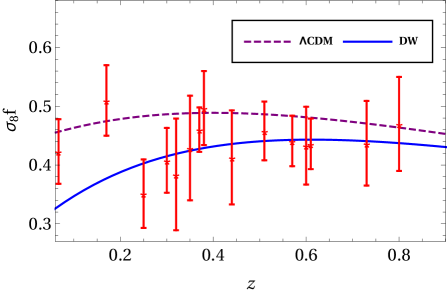
In this work we revisit this problem and show that the localized version of DW model shows a different picture according to which the DW model is not anymore disfavored over CDM and actually gives a significantly better fit to the RSD data. At the same time, the model predicts a slightly lower value of than CDM, in agreement with recent lensing results Ade et al. (2016a); Hildebrandt et al. (2016). It is important to remark that once the background is fixed to reproduce CDM, no more free parameters are left to adjust to the RSD data. Our results disagree with those in Park and Dodelson (2013); Dodelson and Park (2014a). Despite intensive testing, we have been unable to identify the reasons for this discrepancy; we discuss some conjectures below.
We also make one step further and relax the model-dependent assumptions implicit in previous works concerning the initial conditions for the perturbation equation in the matter era. More precisely, we allow the two initial conditions for the linear growth equation to vary (as opposed to fixing them to their standard CDM values). As we will show, however, this improves the fit only marginally.
Throughout the paper, we work in flat space and natural units, i.e. units such that .
II The Model
In Ref. Deser and Woodard (2007) the authors proposed a model in which the Einstein-Hilbert action is nonlocally modified as
| (1) |
where the nonlocal distortion function is a free function of the inverse d’Alembertian acting on the Ricci scalar, . Since this combination is dimensionless, the Lagrangian does not introduce any new energy scale. Variation of (1) with respect to the metric yields the modified Einstein equations,
| (2) |
which in a Friedman-Lemaître-Robertson-Walker (FLRW) background
| (3) |
can be written as
| (4) | |||||
Here, the tensor corresponds to the nonlocal contribution and is given, for the FLRW metric, by the following expressions Deser and Woodard (2007),
| (5) | |||
| (6) |
where and are respectively the energy density and pressure of a perfect fluid. From now on, a comma next to represents a derivative of the function w.r.t its argument. Equations (5-6) can be localized by introducing the auxiliary variables and defined as
| (7) | |||||
| (8) |
With the use of the auxiliary functions and , Eqs. (5-6) can be rewritten as
| (9) | |||||
| (10) |
The DW model has been shown to be capable of reproducing the background evolution given by CDM with Deffayet and Woodard (2009b) by fixing the nonlocal function to
| (11) |
with . This choice fully determines the model and no more free parameters are left.
The dependence of the nonlocal modification on is suggested by quantum radiative corrections Maggiore (2016a) and is triggered mainly at the end of the radiation domination era (since during radiation domination), with a slow evolution afterwards. The interesting question arises then, whether the DW model that gives the same background evolution as CDM, produces also the same behavior at perturbation level. The answer is no, and in the following sections we will see why is it so.
III Perturbation equations
In this section, we introduce the linear scalar perturbation equations for the DW model. Our method of getting perturbation equations is similar to one implemented in Ref. Koivisto (2008) and the results are consistent up to some conventions. Here, we work in the Newtonian gauge, in which scalar perturbations of the metric are given by
| (16) |
We expand the auxiliary fields as and . In general for the anisotropic fluid in the first order of perturbation we have
| (17) | |||||
| (18) | |||||
| (19) |
Here we write the pressure perturbation as , where is the sound speed of the perfect fluid. The density contrast is defined as and is the peculiar velocity field. In the case where the matter content consists of radiation and non-relativistic matter, we have a vanishing anisotropic stress tensor . Below we will write down the linearly perturbed field equations
| (20) | |||||
| (21) |
in Fourier space. The first order perturbation of the component of Friedman equations is given by the following expression:
| (22) | |||||
| (23) | |||||
| (24) | |||||
| (25) |
where the prime stands for derivative with respect to -folding time, . In the following equations we often put ourselves in the sub-horizon limit ( ). To do this, we assume that , and their derivatives, are all of the same order (as indeed can be verified a posteriori) and systematically take the limit of large . For the component, after contracting it with the projecting operator , we get
| (26) |
where represents the anisotropic stress, and where in the sub-horizon limit is
where and , also in the sub-horizon limit, are respectively
| (28) | |||||
| (29) |
where . Moving to the sub-horizon limit we find, for the component,
| (32) | |||||
For the component, after acting with the projection operator, we have
| (33) |
At late times, when the relativistic contribution is small, we can neglect the contribution coming from the anisotropic stress, . So we get
| (34) |
| (35) | |||||
| (36) |
From the covariant conservation law of the energy-momentum tensor, , we get finally the following equations for the matter density perturbation in the sub-horizon limit:
| (37) |
In order to solve this equation we need to find an expression for . This can be done by combining Eqs. (32-34) and Eqs. (35-36). After simple algebraic manipulations we find for the modified gravity function and for the potentials and the following expressions:
| (38) | |||||
| (39) | |||||
| (40) |
Finally, by plugging the expression for from Eq. (39) into Eq. (37), we obtain the -independent growth equation
| (41) |
In order to solve numerically Eqs. (7-8), we set the following initial conditions deep inside radiation-dominated period :
| (42) |
In Ref. Woodard (2014) it was argued that these initial conditions force the homogenous solutions of the localized model to vanish, rendering it equivalent to the nonlocal versions of the DW model. For the growth equation (37), the initial conditions deep into the matter era are taken to be as in pure CDM
| (43) |
where the initial scale factor is taken at redshift . In the next section we generalize the initial conditions.
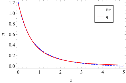
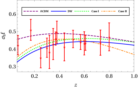
The numerical results for the anisotropic stress and the growth rate fixing (which can be directly extracted from the observational RSD data, see 1) are presented in Figure 1. The DW model fits the data better than CDM ( per d.o.f. equal to 0.736 instead of 0.943, see Tab. 2). The resulting lower normalization, , is in agreement to within 1 with the recent estimates based on lensing Hildebrandt et al. (2016) ( for , Table - column ), contrary to CDM. See also Ade et al. (2016a).
Our results differ significatively from those in Dodelson and Park (2014b), in which lies above the CDM curve, although we agree with their results at the background level. We have not been able to point out the reasons for this discrepancy. One could conjecture it might be due to the fact we are solving a localized version of the model in which the solution depend on the initial conditions on , which in the sub-horizon limit are not free quantities but depend on , and therefore on . However, the quasi-static solution is the attractor solution for large , so it is unlikely that the discrepancy depends on the localization procedure or the quasi-static approximation. Our expression (35) is indeed different from the corresponding quasi-static non-local expression Eq. (29) in Park and Dodelson (2013), but the two expressions coincide asymptotically in time in the limit in which are weakly time-dependent with respect to the rapidly varying sinusoidal function in the integrand for large , conditions that are met in the quasi-static limit. It is still possible that the disagreement is due to the asymptotic equivalence between the local and non-local quasi-static limits not having been reached by the present time.
The behavior of can be approximated with an analytic fit of the form: , where , and are free parameters. We find the following best fit results with a percentage error up to for the quantity in the range : (see Figure 1, left panel).
We have also checked the ghost-freeness condition for the localized theory derived in Ref. Koivisto (2008)
| (44) |
and we found that at all times the condition is violated, while the condition is always satisfied. In Ref. Zhang and Sasaki (2012) the authors have discussed a particular case when the ghost-free condition (44) is satisfied and leads to an interesting cosmology. In the case of tensor-scalar theories it has been shown that the appearance of a ghost mode in the theory’s spectrum will lead to a situation where the effective gravitational constant (in units of ) defined as
| (45) |
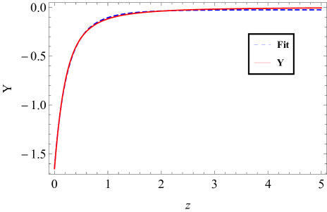
will become negative Amendola (2004). From Figure 2, left panel, we indeed see that is always negative when the non-local contributions are non negligible. This explains why the perturbations grow more slowly than in CDM.
We see that goes negative near the present epoch. This however is only true in our linear approximation. Near non-linear structures, one must assume the existence of a screening mechanism in order to pass local gravity constraints, so that within the screening radius, standard gravity is recovered. This issue has been already discussed in Ref. Woodard (2014) and we refer to that paper for further information. As it was done for the case of , the behaviors of and can be approximated with analytical fits of the polynomial form . The best fit result in the case of , with a percentage error up to for the quantity within , corresponds to (see Figure 2, left panel). For the case of we find the best fit result . with a percentage error up to in the same redshift range, for (see Figure 2, right panel).
IV Sound speed
In order to ascertain that the quasi-static approximation is valid, one has to ensure the absence of gradient instabilities, i.e. whether the sign of the sound-speed of the perturbative-quantities and is positive. To do this, we rewrite Eqs. (30-III) in the following way:
| (46) | |||||
| (47) |
keeping now the derivatives of , but still neglecting and their derivatives with respect to . Now from Eqs. (32-34) in the case of vacuum () we find that
| (48) |
So, by inserting Eq. (48) into Eqs. (46-47) we get finally
| (49) |
and
| (50) |
We can combine these two equations and write them in a matrix form
| (51) |
where is a two by two matrix, defined as
| (52) |
and are the components of the vector . If is positive-definite, the perturbative quantities and have a positive sound-speed independent of the propagation direction. An arbitrary matrix is called positive-definite when it has only positive eigenvalues. The eigenvalues of the matrix are
| (53) |
As mentioned in the previous section, for the DW model one has . On the other hand from the violation of the ghost-free condition (44) we have that . Under these two conditions both eigenvalues of the matrix are always positive and so the matrix is positive-definite. Here, we conclude that the quasi-static approximation is a valid one, which means that the solution based on this approximation is an attractor one and any solution of Eqs. (30-III) should approach it at some point. In Ref. Koivisto (2008), the same procedure is carried out in the Einstein frame, with the same result.
| Survey | References | ||
|---|---|---|---|
| 6dFGRS | Beutler et al. (2012) Beutler et al. (2012) | ||
| LRG-200 | Samushia et al. (2012) Samushia et al. (2012) | ||
| BOSS | Tojeiro et al. (2012)Tojeiro et al. (2012) | ||
| Alam et al. (2016) Alam et al. (2016) | |||
| WiggleZ | Blake (2011) Blake et al. (2012) | ||
| Vipers | De la Torre et al. (2013) de la Torre, S. et al. (2013) | ||
| 2dFGRS | Percival et al. (2004) Percival et al. (2004); Song and Percival (2009) | ||
| LRG | Chuang and Wang (2013) Chuang and Wang (2013) | ||
| LOWZ | Chuang et al. (2013) Chuang et al. (2016) | ||
| CMASS | Samushia et al. (2013) Samushia et al. (2014) |
V Model-independent constraints
Eq. (37) is a second order differential equation for the density contrast and, in order to solve it, we need to specify two initial conditions. The typical choice corresponds to a standard cosmology dominated by pressureless matter at high redshifts, in which . Namely, one assumes
| (54) |
where is some arbitrary initial value of the scale factor outside the range of redshift for which we have observations, say at redshift .
These initial conditions, however, depend on several assumptions about the past: they require, in fact, that matter dominates (), that matter is pressureless, that any decaying mode has been suppressed, and that gravity is Einsteinian. Broadly speaking, there is very little direct proof for any of these assumptions. Let us consider for instance two analytical toy models. In the first, one can imagine that there is a fraction of a homogeneously distributed component along with matter in the past, just like in models of Early Dark Energy (except we are not requiring this component to lead to acceleration at the present). Then the growth of fluctuation obeys the equation
| (55) |
with instead of . In this case, the growth exponent is no longer but rather where
| (56) |
Therefore, if for instance , a value consistent with the analysis in Pettorino et al. (2013) the total growth from to is smaller than the corresponding pure CDM one (we are neglecting here the final accelerated epoch) by a factor
| (57) |
So the existence of a small non-vanishing homogeneous component would produce a value of which would be times smaller than the Planck CDM value.
The second analytical toy case comes from the simplest Brans-Dicke model, parametrized by the Brans-Dicke coupling parameter . In such a case in fact one has during the matter era
| (58) |
rather than unity. If the Brans-Dicke gravity is universal and unscreened, then because of local gravity constraints, and one recovers the standard initial condition. But if the scalar force is not universal and baryons are uncoupled or, alternatively, if the force is screened by a chameleon-like mechanism, then can deviate substantially from standard.
These two toy models show that if one wants to test modified gravity, and not also at the same time the entire CDM paradigm, then one needs to isolate the effects of modified gravity from those that depend on different assumptions. The simplest way to do so is to introduce then two new parameters that correspond to the two initial values of the growth equation (55) and marginalize the likelihood over them. Instead of we adopt the present normalization as first parameter, and
| (59) |
as second free parameter. It is worth mentioning that our approach is of course not completely model independent, in the sense that we still assume that the matter content in the observational range is given by a pressureless perfect fluid and is conserved.
The quantity of interest in this paper is the RSD observable, also called growth rate:
| (60) |
with the amplitude of fluctuations defined as
| (61) |
The current value of the amplitude of fluctuations is estimated through e.g. weak lensing More et al. (2015), the cosmic microwave background power spectrum Ade et al. (2016b) or cluster abundances Ade et al. (2016c). In all these cases the estimate depends, in general, on the choice of a gravity theory. As a consequence the current value of is highly model-dependent.
VI Likelihood analysis
Assuming that and can take any value for modified gravity models, it is of interest to see how the growth rate behaves, in terms of agreement with data, when we allow those two parameters to vary. In what follows we always fix for simplicity.
In general, the likelihood function of a given model (represented by the parameter vector ) with respect to some data is given by with
| (62) |
Here, and are respectively the data and theory vectors, is the covariance matrix and is a normalization constant. The vector contains the measurements of the observable quantity (in our case, the growth rate ) for each point (i.e. each redshift value) and represents the corresponding predictions for that observable. When the data points are independent, takes the form
| (63) |
so the likelihood function may be replaced by the simpler expression
| (64) |
In (64), and are respectively the elements of and , and is the error associated to the measurement .
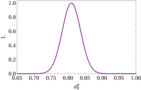
We assume our data points (taken from Alam et al. (2016)) to be independent and thus use (63, 64). We choose to integrate the equation for density perturbations (37) from the redshift . The results of the fits are shown in Table 2, in which we display the deviation given by CDM, by the DW model and by the DW varying first only (Case I) and then varying both (Case II).
| Model | |||
|---|---|---|---|
| CDM | |||
| DW | |||
| DW: case I | |||
| DW: case II | 0.668 |
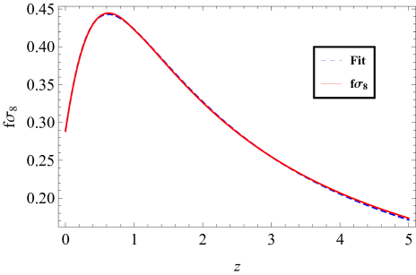
The Case I likelihood for is displayed in Figure (3). For both Case I and Case II, the best-fit yields a better performance compared with CDM, but the improves only marginally upon the no-free parameters DW.
In Figure (4) we show the growth rate given by the three analysis and by CDM.
VII Conclusion
In this work, we have extended the analysis performed in Dodelson and Park (2014b) regarding the predictions of RSD given by the DW model of nonlocal gravity. We have found that the localized version of the theory is not ruled out by the RSD data, as was the case for the previous analysis, and actually leads to a better agreement than the standard CDM cosmology. Ultimately, this behavior is due to the violation of the ghost-free condition. In Ref. Maggiore (2016b) it has been argued that the existence of ghosts in non-local theories does not necessarily rule out the model since the ghost mode is actually “frozen” due to fixed boundary conditions imposed on the model. Interestingly, the predicted value for is in agreement to within 1 with the recent estimates () based on lensing, see e.g. Ade et al. (2016a); Hildebrandt et al. (2016). We have also investigated how much the fit improves when we generalize the initial conditions of the growth rate function, and we find that the improvement is just marginal.
Our perturbation results do not agree with the analysis in Dodelson and Park (2014b), who integrated numerically the equations in their nonlocal form. This could be due to an intrinsic difference between the nonlocal and the localized versions of the DW model, for instance in the way the quasi-static limit is performed. Unfortunately, we have been unable to point out the reason for this discrepancy, notwithstanding extended testing. In any case, we believe the localized version of the DW theory gives interesting predictions on linear perturbation level and deserves further consideration.
Acknowledgements.
We thank S. Doldelson, S. Park, Y. Akrami, J. Rubio, T. Koivisto, V. Pettorino, and S. Casas for several useful discussions. We acknowledge support from DFG through the project TRR33 “The Dark Universe.” H.N. acknowledges financial support from DAAD through the program “Forschungsstipendium für Doktoranden und Nachwuchswissenschaftler.”References
- Riess et al. (1998) A. G. Riess et al. (Supernova Search Team), Astron. J. 116, 1009 (1998), eprint astro-ph/9805201.
- Perlmutter et al. (1999) S. Perlmutter et al. (Supernova Cosmology Project), Astrophys. J. 517, 565 (1999), eprint astro-ph/9812133.
- Sherwin et al. (2011) B. D. Sherwin et al., Phys. Rev. Lett. 107, 021302 (2011), eprint 1105.0419.
- Dunkley et al. (2009) J. Dunkley et al. (WMAP), Astrophys. J. Suppl. 180, 306 (2009), eprint 0803.0586.
- Komatsu et al. (2009) E. Komatsu et al. (WMAP), Astrophys. J. Suppl. 180, 330 (2009), eprint 0803.0547.
- van Engelen et al. (2012) A. van Engelen et al., Astrophys. J. 756, 142 (2012), eprint 1202.0546.
- Scranton et al. (2003) R. Scranton et al. (SDSS) (2003), eprint astro-ph/0307335.
- Sanchez et al. (2012) A. G. Sanchez et al., Mon. Not. Roy. Astron. Soc. 425, 415 (2012), eprint 1203.6616.
- Deser and Woodard (2007) S. Deser and R. P. Woodard, Physical Review Letters 99 (2007), ISSN 0031-9007, 1079-7114, arXiv: 0706.2151, URL http://arxiv.org/abs/0706.2151.
- Deffayet and Woodard (2009a) C. Deffayet and R. P. Woodard, Journal of Cosmology and Astroparticle Physics 2009, 023 (2009a), ISSN 1475-7516, arXiv: 0904.0961, URL http://arxiv.org/abs/0904.0961.
- Koivisto (2008) T. S. Koivisto, Phys. Rev. D78, 123505 (2008), eprint 0807.3778.
- Nojiri et al. (2011) S. Nojiri, S. D. Odintsov, M. Sasaki, and Y.-l. Zhang, Phys. Lett. B696, 278 (2011), eprint 1010.5375.
- Deser and Woodard (2013) S. Deser and R. P. Woodard, JCAP 1311, 036 (2013), eprint 1307.6639.
- Park and Dodelson (2013) S. Park and S. Dodelson, Physical Review D 87 (2013), ISSN 1550-7998, 1550-2368, arXiv: 1209.0836, URL http://arxiv.org/abs/1209.0836.
- Dodelson and Park (2014a) S. Dodelson and S. Park, Physical Review D 90 (2014a), ISSN 1550-7998, 1550-2368, arXiv: 1310.4329, URL http://arxiv.org/abs/1310.4329.
- Ade et al. (2016a) P. A. R. Ade et al. (Planck), Astron. Astrophys. 594, A14 (2016a), eprint 1502.01590.
- Hildebrandt et al. (2016) H. Hildebrandt et al. (2016), eprint 1606.05338.
- Deffayet and Woodard (2009b) C. Deffayet and R. P. Woodard, JCAP 0908, 023 (2009b), eprint 0904.0961.
- Maggiore (2016a) M. Maggiore, Phys. Rev. D93, 063008 (2016a).
- Woodard (2014) R. P. Woodard, Found. Phys. 44, 213 (2014), eprint 1401.0254.
- Dodelson and Park (2014b) S. Dodelson and S. Park, Phys. Rev. D90, 043535 (2014b), eprint 1310.4329.
- Zhang and Sasaki (2012) Y.-l. Zhang and M. Sasaki, Int. J. Mod. Phys. D21, 1250006 (2012), eprint 1108.2112.
- Amendola (2004) L. Amendola, Physical Review Letters 93, 181102 (2004).
- Beutler et al. (2012) F. Beutler, C. Blake, M. Colless, D. H. Jones, L. Staveley-Smith, G. B. Poole, L. Campbell, Q. Parker, W. Saunders, and F. Watson, MNRAS 423, 3430 (2012), eprint 1204.4725.
- Samushia et al. (2012) L. Samushia, W. J. Percival, and A. Raccanelli, Mon. Not. Roy. Astron. Soc. 420, 2102 (2012), eprint 1102.1014.
- Tojeiro et al. (2012) R. Tojeiro, W. Percival, J. Brinkmann, J. Brownstein, D. Eisenstein, M. Manera, C. Maraston, C. Mcbride, D. Muna, B. Reid, et al., Monthly Notices of the Royal Astronomical Society 424, 2339 (2012), ISSN 0035-8711.
- Alam et al. (2016) S. Alam et al. (BOSS), Submitted to: Mon. Not. Roy. Astron. Soc. (2016), eprint 1607.03155.
- Blake et al. (2012) C. Blake et al., Mon. Not. Roy. Astron. Soc. 425, 405 (2012), eprint 1204.3674.
- de la Torre, S. et al. (2013) de la Torre, S., Guzzo, L., Peacock, J. A., Branchini, E., Iovino, A., Granett, B. R., Abbas, U., Adami, C., Arnouts, S., Bel, J., et al., Astronom.Astrophy. 557, A54 (2013), URL http://dx.doi.org/10.1051/0004-6361/201321463.
- Percival et al. (2004) W. J. Percival et al. (2dFGRS), Mon. Not. Roy. Astron. Soc. 353, 1201 (2004), eprint astro-ph/0406513.
- Song and Percival (2009) Y.-S. Song and W. J. Percival, JCAP 0910, 004 (2009), eprint 0807.0810.
- Chuang and Wang (2013) C.-H. Chuang and Y. Wang, Mon. Not. Roy. Astron. Soc. 435, 255 (2013), eprint 1209.0210.
- Chuang et al. (2016) C.-H. Chuang et al., Mon. Not. Roy. Astron. Soc. 461, 3781 (2016), eprint 1312.4889.
- Samushia et al. (2014) L. Samushia et al., Mon. Not. Roy. Astron. Soc. 439, 3504 (2014), eprint 1312.4899.
- Pettorino et al. (2013) V. Pettorino, L. Amendola, and C. Wetterich, Phys. Rev. D 87, 083009 (2013), eprint 1301.5279.
- More et al. (2015) S. More, H. Miyatake, R. Mandelbaum, M. Takada, D. Spergel, J. Brownstein, and D. P. Schneider, Astrophys. J. 806, 2 (2015), eprint 1407.1856.
- Ade et al. (2016b) P. A. R. Ade et al. (Planck), Astron. Astrophys. 594, A13 (2016b), eprint 1502.01589.
- Ade et al. (2016c) P. A. R. Ade et al. (Planck), Astron. Astrophys. 594, A24 (2016c), eprint 1502.01597.
- Maggiore (2016b) M. Maggiore (2016b), eprint 1606.08784.