Design and optimization of a portable LQCD Monte Carlo code using OpenACC

Abstract

The present panorama of HPC architectures is extremely heterogeneous, ranging from traditional multi-core CPU processors, supporting a wide class of applications but delivering moderate computing performance, to many-core GPUs, exploiting aggressive data-parallelism and delivering higher performances for streaming computing applications. In this scenario, code portability (and performance portability) become necessary for easy maintainability of applications; this is very relevant in scientific computing where code changes are very frequent, making it tedious and prone to error to keep different code versions aligned. In this work we present the design and optimization of a state-of-the-art production-level LQCD Monte Carlo application, using the directive-based OpenACC programming model. OpenACC abstracts parallel programming to a descriptive level, relieving programmers from specifying how codes should be mapped onto the target architecture. We describe the implementation of a code fully written in OpenACC, and show that we are able to target several different architectures, including state-of-the-art traditional CPUs and GPUs, with the same code. We also measure performance, evaluating the computing efficiency of our OpenACC code on several architectures, comparing with GPU-specific implementations and showing that a good level of performance-portability can be reached.

PACS Nos.: 07.05.Bx 12.38.Gc

1 Introduction and related works

The use of processors based on multi- and many-core architectures is a common option in High Performance Computing (HPC). Several variants of these processors exist, differing mainly in the number and architecture of the cores integrated in a single silicon die.

Conventional CPUs integrate tens of fat cores sharing a large on-chip cache. Fat cores include several levels of caches and complex control structures, able to perform hardware optimization techniques (branch-speculation, instruction scheduling, register renaming, etc). Vector instructions are also supported by these cores, with a moderate level of data parallelism: 2 to 4 vector elements are processed by one vector instruction. This architecture is reasonably efficient for many type of regular and non-regular applications and delivers a level of performance of the order of hundreds of GigaFlops per processor.

On the other side of the spectrum we have Graphics Processor Units (GPU), available as accelerator boards attached to conventional CPUs. GPUs integrate thousands of slim cores able to efficiently support regular streams of computation, and deliver performances of the order of several TeraFlops. GPUs are extremely aggressive in terms of data-parallelism, implementing vector units with large vector sizes (16 and 32 words are presently available options).

Midway between these two architectures, we have the Intel Many Integrated Cores (MIC) architecture based on several tens of slim cores. In this case, cores are similar to their fat counterparts, but their design has been simplified removing many hardware control structures (instruction scheduler, register renaming, etc) and adopting wider vector units, able to process up to 4 or 8 vector elements in parallel.

Large scale computing centers today have not reached a common consensus on the “best” processor option for HPC systems, also because system choices are driven not only by application performances, but also by cost of ownership and energy aspects which are becoming increasingly critical parameters[1]. Several computing centers do adopt machines based on GPUs, but other ones prefer to stay on more traditional CPUs, offering a lower peak performance, but better computing efficiency for a wider range of applications.

In this scenario, the development of applications would greatly benefit from the availability of a unique code version, written in an appropriate programming framework, able to offer portability, in terms of code and performance, across several present and possibly future state-of-the-art processor architectures. A single code version, portable across several architectures, is of great convenience in particular for scientific applications, where code changes and development iterations are very frequent, so keeping several architecture-specific code versions up-to-date is a tedious and error prone effort[2, 3].

Directives based programming models are going exactly in this direction, abstracting parallel programming to a descriptive level as opposite to a prescriptive level, where programmers must specify how the code should be mapped onto the target machine. OpenMP[4] and OpenACC[5] are among the most common such programming models, already used by a wide scientific community. Both are based on directives: OpenMP was introduced to manage parallelism on traditional multi-core CPUs, while OpenACC is mainly used to target GPUs (although designed to be architecture agnostic)[6]. These two frameworks are in fact converging and extending their scope to cover a large subset of HPC applications and architectures: OpenMP version 4 has been designed to support also accelerators, while compilers supporting OpenACC (such as the PGI[8]) are starting to use directives also to target multi-core CPUs.

In this work we describe the implementation of a Lattice QCD (LQCD) Monte Carlo code designed to be portable and efficient across several architectures. LQCD simulations represent a typical and well known HPC grand challenge, with physics results strongly limited by available computational resources[9, 10]; over the years, several generations of parallel machines, optimized for LQCD, have been developed[11, 12, 13, 14, 15], while the development of LQCD codes running on many core architectures, in particular GPUs, has seen large efforts in the last 10 years[16, 17, 18, 19, 20, 21, 22, 23]. Our goal is to have just one code able to run on several processors without any major code changes, and possibly to have roughly the same level of efficiency, looking for an acceptable trade-off between portability and efficiency[3, 7].

As a programming model we have selected OpenACC, as it currently has a wider compiler support, in particular targeting NVIDIA GPUs, which are widely used in HPC clusters and commonly used for scientific computations. OpenACC has been successfully used to port and run other scientific codes, such as Lattice Boltzmann applications[24, 25, 26] in computational fluid-dynamics, showing a good level of code and performance portability on several architectures. The migration of our code to OpenMP4, if needed, as soon as compiler support becomes more mature, is expected to be a simple additional effort.

We have developed a code with all key features for a state-of-the-art simulations of QCD with dynamical fermions. Using this code as a user test case, we assess: i) if it is possible to write the code in such a way that the most computationally critical kernels can be executed on accelerators, as in previous CUDA implementations[21]; ii) how many of the presently available multi and many-core architectures can be really used; iii) how efficient are these codes, and in particular what is the price to pay in terms of performance with respect to a code written and optimized for a specific architecture (e.g., using CUDA for GPUs).

We believe that our work is a non trivial step forward in the development of a fully portable production-grade LQCD Monte Carlo code, using the OpenACC programming model. An earlier paper[27] presented tests of selected portions of an OpenACC LQCD implementation on Fermi and K20 NVIDIA GPUs, comparing performances with an OpenMP implementation for CPUs. Similarly, in a preliminary study[2], we compared the performance of selected kernels of a full simulation, written in OpenACC, with an equivalent CUDA implementation, on a K20 NVIDIA GPU. In this work, we extend the use of OpenACC in several new directions: i) we show the portability of a complete implementation across several architectures; ii) we show performance figures for the same OpenACC code on a variety of multi and many-core processors, including the most recent GPUs like the K80 and the recently released P100; iii) we compare results with a previous implementation of the same full application written in CUDA[21].

The remainder of the paper is organized as follows: in Section 2 we give a brief introduction to LQCD and to the main computational aspects of our application; in Section 3 we highlight recent developments in HPC hardware and programming tools; in Section 4 we describe the OpenACC implementation of our code; in Section 5 we analyze our results; finally, Section 6, contains our concluding remarks.

2 Numerical challenges of Lattice QCD

Quantum Chromodynamics (QCD) is the quantum field theory that describes strong interactions in the Standard Model of particle physics. It is a non-abelian gauge theory, based on the $SU(3)$ group (the “color” group), describing the interactions of six different species (“flavors”) of quarks, mediated by $8$ vector bosons, the “gluons”.

In principle QCD is not different from the theory that describes other sectors of the Standard Model (i.e. the electroweak interaction); however, strong interactions are indeed strong, i.e. the coupling constant of QCD is generically not small. Asymptotic freedom ensures that the coupling constant gets smaller and smaller as the energy scale increases (a summary of experimental results is available in §9.4 of the Particle Data Group review[28]), but a wealth of interesting phenomena take place for energies well below the perturbative regime; a systematically improvable computational scheme, that does not rely on the smallness of the coupling constant, is needed to study this phenomenology from first principles. Lattice QCD provides such a scheme.

LQCD uses the Feynman path-integral quantization and approximates the infinite dimensional path-integral by a finite dimensional integral: continuous space-time is replaced by a finite lattice of sizes $L_{t}$, $L_{x}$, $L_{y}$, $L_{z}$ and lattice spacing $a$. In order to maintain gauge invariance, the variables $U_{\mu}(n)$ associated with the gauge fields are elements of the $SU(3)$ group and live on the links of the lattice; the quark fields $\psi(n)$ live on the lattice sites and transform under the gauge group as $3-$dimensional complex vectors[29]. The fundamental problem of LQCD is the evaluation of expectation values of given functions of the fields, $O[U]$, that is integrals of the form

$$\langle\hat{O}\rangle=\frac{1}{Z}\int\mathscr{D}UO[U]\det(M[U])e^{-S_{g}[U]}\ ,\quad Z=\int\mathscr{D}U\det(M[U])e^{-S_{g}[U]}\ ;$$ (1)

the exponent $S_{g}$ is the discretization of the action of the gauge fields (usually written as a sum of traces of products of $U_{\mu}(n)$ along closed loops) and $\det(M)$ describes the gluon-quark interaction. Here, $M[U]$ is a large and sparse structured matrix (i.e. containing both space-time and color indexes) which is the discretization of the continuum fermion operator $M\sim m\,{\rm I}+D$ where $m$ is the fermion mass, multiplying the identity operator, and $D$ is the Dirac operator, which is constructed in terms of covariant derivatives. The integral in $\mathscr{D}U$ extends over all the $U_{\mu}(n)$ variables on the lattice using the Haar measure of $SU(3)$. Eq. (1) refers to a single quark species (flavor); in the realistic case of multiple flavors, one has to introduce a separate determinant for each flavor.

This formulation makes contact with a standard problem in statistical mechanics: importance sampling of the distribution $\det(M[U])e^{-S_{g}[U]}$. What is non-standard is the form of this distribution and in particular the presence of the determinant. The best strategy devised so far to cope with this problem is to introduce the so called pseudofermion fields[30] $\phi$ and rewrite the integral as follows:

$$\int\mathscr{D}UO[U]\det(M[U])e^{-S_{g}[U]}\propto\int\mathscr{D}U\mathscr{D}\phi\,O[U]\exp\left(-S_{g}[U]-\phi^{{\dagger}}M[U]^{-1}\phi\right)\ ;$$ (2)

the action is still a non-local function of the field variables, but the computational burden required for the solution of a large sparse linear system is much lower than the one needed for the computation of its determinant.

The explicit form of $S_{g}[U]$ and $M[U]$ is not fully determined, as these functions only have the constraint to go over to the correct continuum limit as the lattice spacing goes to zero. Much in the same way as several discretization schemes exist for the numerical solution of a partial differential equation, several discretization schemes of the QCD action exist. In this paper we consider a specific state-of-the-art discretization, the tree-level Symanzik improved action[31, 32] for the gauge part and the stout-improved[33] “staggered” action for the fermion part. Staggered actions have a residual degeneracy, that has to be removed by taking the $4-$th root of the determinant. So, Eq. (2) becomes in the staggered case

$$\int\mathscr{D}U\mathscr{D}\phi\,O[U]\exp\big{(}-S_{g}[U]-\phi^{{\dagger}}M[U]^{-1/4}\phi\big{)}\ .$$ (3)

2.1 Why LQCD is a computational grand challenge

The physical system that one would like to simulate by the lattice box has a characteristic physical length $\xi$, which is of the order of $10^{-15}$ m. In order to reduce systematic effects related to discretization and to the finite box size, one would like that, at the same time, the lattice spacing $a$ be much smaller, and the box size $La$ much larger than $\xi$, i.e. $a\ll\xi\ll La$. Making the reasonable approximation that $\ll$ translates into one order of magnitude means that the number of sites in each direction should be $\simeq 10^{2}$; the corresponding fermion matrix, considering also internal (e.g., color) indexes, has a dimension slightly exceeding $10^{8}\times 10^{8}$; note that it is a sparse matrix, since the discretization of the Dirac operator $D$ connects only neighbor lattice sites. In finite temperature simulations the size of the lattice is typically smaller, since in that case the temporal direction is shortened and equal to the inverse of the temperature, $1/T$.

The most computationally demanding task in the typical LQCD algorithm is the solution of a linear system involving the fermion matrix $M$. The numerical difficulty of this problem is fixed by the condition number of $M$, hence, since the highest eigenvalue is typically $O(1)$, by the smallest eigenvalue of $M$. Here the physical properties of QCD play a significant role: the eigenvalues of the Dirac operator are dense around zero, a property related to the so-called spontaneous breaking of chiral symmetry, so the smallest eigenvalue is set by $am$ where $m$ is quark mass. Since Nature provides us with two quark flavors ($u$ and $d$ quarks) whose mass is significantly lower (by two orders of magnitude) than other energy scales of the theory, typical values of $am$ are typically very small, resulting in a bad condition number ($\kappa\gtrsim 10^{5}$ being a typical value). Also regarding this aspect, the situation becomes better when one is interested in the regime of very high temperatures, since in that case the spontaneous breaking of chiral symmetry disappears, the minimum eigenvalue of $D$ is non-zero, and the condition number significantly improves.

2.2 Numerical algorithms for LQCD

In LQCD, the usual local updates adopted in statistical mechanics scale badly with the volume, as the action of Eq. (2) is non-local. This problem is partly solved by the Hybrid Monte Carlo (HMC) algorithm[34]; in HMC we associate fake conjugate momenta – entering quadratically in the action – to each degree of freedom of the system. For an $SU(3)$ gauge theory, momenta conjugate to the link variable are again $3\times 3$ matrices $H_{\mu}(n)$ associated to each link of the lattice, this time living in the group algebra (hence Hermitian and traceless). Eq. (3) is rewritten as

$$\int\mathscr{D}U\mathscr{D}\phi\mathscr{D}HO[U]\exp\left(-\frac{1}{2}H^{2}-S_{g}[U]-\phi^{{\dagger}}M[U]^{-1/4}\phi\right)\ ,$$ (4)

where the momenta term is a shorthand to indicate the sum of $-{\rm Tr}(H_{\mu}(n)^{2})/2$ over the whole lattice. The update then proceeds as follows:

1. random gaussian initial momenta $H$ and pseudofermions $\phi$ are generated;

2. starting from the initial configuration and momenta $(U,H)$, a new state $(U^{\prime},H^{\prime})$ is generated by integrating the equations of motion;

3. the new state $(U^{\prime},H^{\prime})$ is accepted with probability $e^{-\Delta S}$, where $\Delta S$ is the change of the total (i.e. included the momenta) action.

Step 2 is an unphysical evolution in a fictitious time and, under mild conditions on the numerical integration of the equations of motion, it can be shown to satisfy the detailed balance principle[34, 35], so it provides a stochastically exact way to estimate the integral in Eq. (2). The more time consuming steps of the update are the ones that involve the non-local term in the exponent of Eq. (2). In particular, the most time consuming single step of the whole algorithm is the solution of a linear system

$$M[U]\varphi=b\,.$$ (5)

This calculation is needed to compute the forces appearing in the equations of motion and also to evaluate $\Delta S$, and one usually resorts to Krylov solvers. In the case of staggered fermions, corresponding to Eq. (3), it is customary to use the so-called Rational HMC (RHMC) algorithm[36, 37, 38], in which the algebraic matrix function appearing in Eq. (3) is approximated to machine precision by a rational function. In this case one replaces Eq. (5) by $r$ equations ($r$ is the order of the approximation adopted)

$$(M[U]+\sigma_{i})\varphi_{i}=b\ ,\quad i\in\{1,\ldots,r\}\ ,$$ (6)

where the real numbers $\sigma_{i}$ are the poles of the rational approximations. These equations can again be solved by using Krylov methods: by exploiting the shift-invariance of the Krylov subspace it is possible to write efficient algorithms that solve all the equations appearing in (6) at the same time, using at each iteration only one matrix-vector product[39, 40].

For most of the discretizations adopted in QCD (and in particular for the one we use), the matrix $M[U]$ can be written in block form

$$M=m\,I+\left(\begin{array}[]{cc}0&D_{oe}\\ D_{eo}&0\end{array}\right),\qquad D_{oe}^{{\dagger}}=-D_{eo}\ ;$$ (7)

matrices $D_{oe}$ and $D_{eo}$ connect only even and odd sites. It is thus convenient to use an even/odd preconditioning[41, 42]; in this case, Eq. (5) is replaced by:

$$(m^{2}\,I-D_{eo}D_{oe})\varphi_{e}=b_{e};$$ (8)

$\varphi_{e}$ is defined only on even sites and the matrix is positive definite (because of Eq. (7)), so we can use the simplest of the Krylov solvers: the conjugate gradient (or its shifted counterpart).

Over the years, many improvements of this basic scheme have been developed; these are instrumental in reducing the computational cost of actual simulations but their implementation is straightforward, once the basic steps of the “naive” code are ready. For this reason we will not discuss in the following the details of multi-step integrators[43, 44], improved integrators[45, 46, 47], multiple pseudofermions[37] or the use of different rational approximations and stopping residuals in different parts of the HMC[38], even if our code uses all these improvements.

2.3 Data structures and computational challenges

Our most important data structures are the collection of all gauge variables $U_{\mu}(n)$ (elements of the group of $SU(3)$ matrices, one for each link of the four-dimensional lattice) and of the pseudofermion fields $\phi(n)$ ($3-$dimensional complex vectors, one for each even site of the lattice when using the even/odd preconditioning). We also need many derived and temporary data structures, such as:

1. the configurations corresponding to different stout levels ($U_{\mu}^{(k)}(n)$, again $SU(3)$ matrices), used in the computation of the force (typically less than five stout levels are used) and the momenta configuration (which are $3\times 3$ Hermitian traceless matrices);

2. some auxiliary structures needed to compute the force acting on the gauge variables, like the so called “staples” $\Sigma_{\mu}^{(k)}(n)$ and the $\Gamma_{\mu}(n)$ and $\Lambda_{\mu}(n)$ matrices[33]; $\Sigma_{\mu}^{(k)}(n)$ and $\Gamma_{\mu}(n)$ are generic $3\times 3$ complex matrices and $\Lambda_{\mu}(n)$ are $3\times 3$ Hermitian traceless matrices;

3. the solutions $\varphi_{i}$ of Eq. (6) and some auxiliary pseudofermion-like structure needed in the Krylov solver.

At the lowest level, almost all functions repeatedly multiply two $3\times 3$ complex matrices (e.g., in the update of the gauge part), or a $3\times 3$ complex matrix and a $3-$dimensional complex vector (e.g., in the Krylov solver) or compute dot products and linear combinations of complex $3-$vectors. All these operations have low computational intensity, so it is convenient to compress as much as possible all basic structures by exploiting their algebraic properties. The prototypical example is $U_{\mu}(n)$: one only stores the first two rows of the matrix and recovers the third one on the fly as the complex conjugate of the wedge product of the first two rows[48]. This overhead is negligible with respect to the gain induced, at least for GPUs, by the reduction of the memory transfer[49, 50].

At a higher level the single most time consuming function is the Krylov solver, which may take $40\dots 80\%$ of the total execution time of a realistic simulation (depending e.g. on the value of the temperature) and consists basically of repeated applications of the $D_{oe}$ and $D_{eo}$ matrices defined in Eq. (7), together with some linear algebra on the pseudofermion vectors (basically zaxpy-like functions). An efficient implementation of $D_{eo}$ and $D_{oe}$ multiplies is then of paramount importance, the effectiveness of this operation being often taken as a key figure of merit in the LQCD community.

3 Current trends in HPC

There is a clear trend in high-performance computing (HPC) to adopt multi-core processors and accelerator-based platforms. Typical HPC systems today are clusters of computing nodes interconnected by fast low-latency communication networks, e.g. Infiniband. Each node typically has two standard multi-core CPUs, each attached to one or more accelerators, either Graphic Processing Unit (GPU) or many-core systems.

Recent development trends see a common path to performance for CPUs and accelerators, based on an increasing number of independent cores and on wider vector processing facilities within each core. In this common landscape, accelerators offer additional computing performance and better energy efficiency by further pushing the granularity of their data paths and using a larger fraction of their transistors for computational data paths, as opposed to control and memory structures. As a consequence, even if CPUs are more tolerant for intrinsically unstructured and irregular codes, in both class of processors computing efficiency goes through careful exploitation of the parallelism available in the target applications combined with a regular and (almost) branch-free scheduling of operations.

This remark supports our attempt to write just one LQCD code which is not only portable, but also efficiency-portable across a large number of state-of-the-art CPUs and accelerators. In this paper we consider Intel multi-core CPUs, and NVIDIA and AMD GPUs, commonly used today by many scientific HPC communities. Table 3 summarizes some key features of the systems we have used[51, 52, 53, 54], that we describe very briefly in the following.

Selected hardware features of some of the processors used in this work: the Xeon-E5 systems are two recent multi-core CPUs based on the Haswell and Broadwell architecture, the K80 GPU is based on the Kepler architecture while the P100 GPU adopts the Pascal architecture. The FirePro W9100 is an AMD GPU, based on the Hawaii architecture. Xeon E5-2630 v3 Xeon E5-2697 v4 K80-GK210 P100 FirePro W9100 Year 2014 2016 2014 2016 2014 Architetcure Haswell Broadwell Kepler Pascal Hawaii #physical-cores / SMs 8 18 13 $\times$ 2 56 44 #logical-cores / CUDA-cores 16 26 2496 $\times$ 2 3584 2816 Nominal Clock (GHz) 2.4 2.3 562 1328 930 Nominal DP performance (Gflops) $\approx 300$ $\approx 650$ 935 $\times$ 2 4759 2620 LL cache (MB) 20 45 1.68 4 1.00 Total memory supported (GB) 768 1540 12 $\times$ 2 16 16 Peak mem. BW (ECC-off) (GB/s) 69 76.8 240 $\times$ 2 732 320

Intel Xeon-E5 architectures are conventional x86 multi-core architectures. We have used two generations of these processors, differing for the number of cores and for the amount of integrated last-level cache. Performances in both cases rely on the ability of the application to run on all cores and to use 256-bit vector instructions.

NVIDIA GPUs are also multi-core processors. A GPU hosts several Streaming Multiprocessors (SM), which in turn include several (depending on the specific architecture) compute units called CUDA-cores. At each clock-cycle SMs execute multiple warps, i.e. groups of 32 instructions, belonging to different CUDA-threads, which are executed in Single Instructions Multiple Threads (SIMT) fashion. SIMT is similar to SIMD execution but more flexible, e.g. different CUDA-threads of a SIMT-group are allowed to take different branches of the code, although at a performance penalty. Each CUDA-thread has access to its copy of registers and context switches are almost at zero cost. This structure has remained stable across several generations with minor improvements. The NVIDIA K80 has two GK210 GPUs; each GPU has 13 Next Generation Streaming Multiprocessor, (SMX) running at a base frequency of $562$ MHz that can be increased to $875$ MHz under specific condition of work-load and power. The corresponding aggregate peak performance of the two GK210 units is then $1.87$ and $2.91$ TFlops in double precision. The peak memory bandwidth is $240$ GB/s considerably higher compared to that of E5-Xeon CPUs. The GP100 GPU, based on the Pascal architecture, has recently become available. It has 56 streaming processors running at base-frequency of $1.3$ that can be increased to $1.48$ GHz, delivering a peak double-precision performance of $4.76$ and $5.30$ Tflops. Peak memory bandwidth has been increased to $732$ GB/s.

The AMD GPUs are conceptually similar to NVIDIA GPU. The AMD FirePro W9100 has 44 processing units, each one with 64 compute units (stream processors), running at $930$ MHz. This board delivers a peak double-precision performance of $2.6$ Tflops, and has a peak memory-bandwidth of $320$ GB/s.

Native programming models, commonly used for the systems shown in Table 3, differ in several aspects.

For Xeon-E5 CPUs, the most common models are OpenMP and OpenMPI. Both models support core-parallelism, running one thread or one MPI process per logical core. Moreover OpenMP is a directive based programming model, and allows to exploit vector-parallelism properly annotating for-loops that can be parallelized[4].

On GPUs, the native programming model is strongly based on data-parallel models, with one thread typically processing one element of the application data domain. This helps exploit all available parallelism of the algorithm and hide latencies by switching among threads waiting for data coming from memory and threads ready to run. The native language is CUDA-C for NVIDIA GPUs and OpenCL for AMD systems. Both languages have a very similar programming model but use a slight different terminology; for instance, on OpenCL the CUDA-thread is called work-item, the CUDA-block work-group, and the CUDA-kernel is a device program. A CUDA-C or OpenCL program consists of one or more functions that run either on the host, a standard CPU, or on a GPU. Functions that exhibits no (or limited) parallelism run on the host, while those exhibiting a large degree of data parallelism can go onto the GPU. The program is a modified C (or C++, Fortran) program including keyword extensions defining data parallel functions, called kernels or device programs. Kernel functions typically translate into a large number of threads, i.e. a large number of independent operations processing independent data items. Threads are grouped into blocks which in turn form the execution grid. When all threads of a kernel complete their execution, the corresponding grid terminates. Since threads run in parallel with host CPU threads, it is possible to overlap in time processing on the host and the accelerator.

New programming approaches are now emerging, mainly based on directives, moving the coding abstraction layer at an higher lever, over the hardware details. These approaches should make code development easier on heterogeneous computing systems[5], simplifying the porting of existing codes on different architectures. OpenACC is one such programming models, increasingly used by several scientific communities. OpenACC is based on pragma directives that help the compiler to identify those parts of the code that can be implemented as parallel functions and offloaded on the accelerator or divided among CPU cores. The actual construction of the parallel code is left to the compiler making, at least in principle, the same code portable without modifications across different architectures and possibly offering more opportunities for performance portability. This make OpenACC more descriptive compared to CUDA and OpenCL which are more prescriptive oriented.

Listing 1: Sample OpenACC code computing a saxpy function on vectors $x$ and $y$. The pragma clauses control data transfers between host and accelerator and identify the code regions to be run on the accelerator.

⬇

#pragma acc data copyin(x), copy(y) {

#pragma acc kernels present(x) present(y) async(1)

#pragma acc loop vector(256)

for (int i = 0; i < N; ++i)

y[i] = a*x[i] + y[i];

#pragma wait(1);

}

Listing 1 shows an example of the saxpy operation of the Basic Linear Algebra Subprogram (BLAS) set coded in OpenACC. The pragma acc kernels clause identifies the code fragment running on the accelerator, while pragma acc loop… specifies that the iterations of the for-loop can execute in parallel.

The standard defines several directives, allowing a fine tuning of applications. As an example, the number of threads launched by each device function and their grouping can be tuned by the vector, worker and gang directives, in a similar fashion as setting the number of work-items and work-groups in CUDA. Data transfers between host and device memories are automatically generated, and occur on entering and exiting the annotated code regions. Several data directives are available to allow the programmer to optimize data transfers, e.g. overlapping transfers and computation. For example, in Listing 1 the clause copyin(ptr) copies the array pointed by ptr from the host memory into the accelerator memory before entering the following code region; while copy(ptr) perform the additional operation of copying it also back to the host memory after leaving the code region. An asynchronous directive async is also available, instructing the compiler to generate asynchronous data transfers or device function executions; a corresponding clause (i.e. #pragma wait(queue)) allows to wait for completion.

OpenACC is similar to the OpenMP (Open Multi-Processing) framework widely used to manage parallel codes on multi-core CPUs in several ways[6]; both frameworks are directive based, but OpenACC targets accelerators in general, while at this stage OpenMP targets mainly multi-core CPUs; the latest release of OpenMP4 standard has introduced directives to manage also accelerators, but currently, compilers support is still limited. Regular C/C++ or Fortran code, already developed and tested on traditional CPU architectures, can be annotated with OpenACC pragma directives (e.g. parallel or kernels clauses) to instruct the compiler to transform loop iterations into distinct threads, belonging to one or more functions to run on an accelerator. Ultimately, OpenACC is particularly well suited for developing scientific HPC codes for several reasons:

• it is highly hardware agnostic, allowing to target several architectures, GPUs and CPUs, allowing to develop and maintain one single code version;

• the programming overhead to offload code regions to accelerators is limited to few pragma lines, in contrast to CUDA and in particular OpenCL verbosity;

• the code annotated with OpenACC pragmas can be still compiled and run as plain C code, ignoring the pragma directives.

4 OpenACC implementation of Lattice QCD

In this section we describe the OpenACC implementation of our LQCD code. We first describe the data structures used, then we highlight the most important OpenACC-related details of our implementation. In writing the OpenACC version, we started from our previous code implementations[2]: a C++/CUDA[21] developed for NVIDIA GPUs aggressively optimized with CUDA-specific features, and a C++ one, developed using OpenMP and MPI directives, targeting large CPU clusters[55].

4.1 Memory allocation and data structures

Data structures have a strong impact on performance[2, 56] and can hardly be changed on an existing implementation: their design is in fact a critical step in the implementation of a new code. We have analyzed in depth the impact of data-structures for LQCD on different architectures (i.e. a GPU and a couple of CPUs), confirming that the Structure of Arrays (SoA) memory data layout is preferred when using GPUs, but also when using modern CPUs[2]. This is due to the fact that the SoA format allows vector units to process many sites of the application domain (the lattice, in our case) in parallel, favoring architectures with long vector units (e.g. with wide SIMD instructions). Modern CPUs tend indeed to have longer vector units than older ones and we expect this trend to continue in the future. For this reason, all data structures related to lattice sites in our code follow the SoA paradigm.

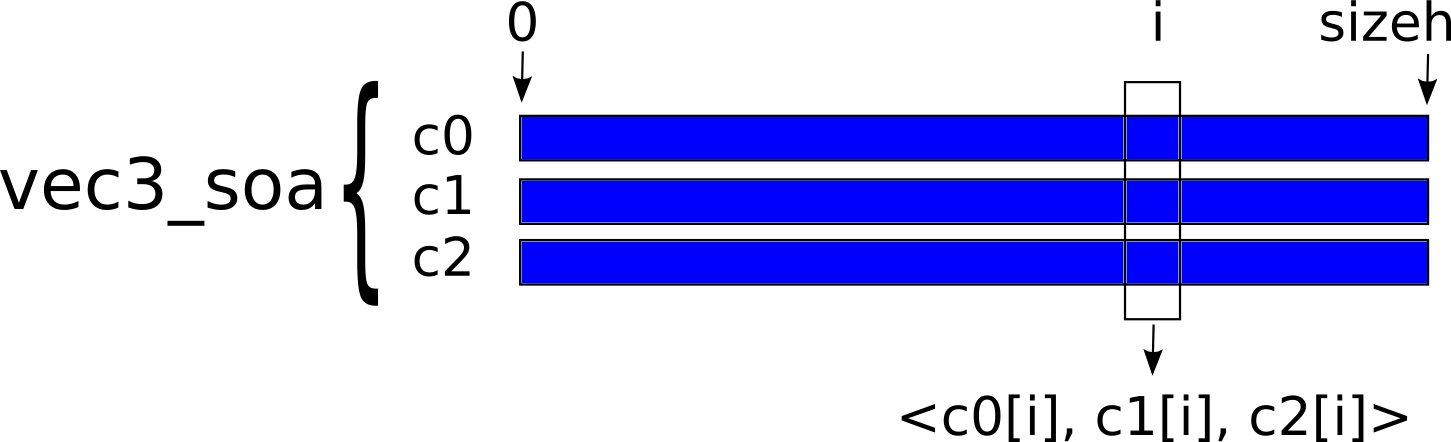
Figure 1: Memory data layout for structure vec3_soa. Each component $i$ of each array c0, c1 and c2 is a C99 complex value. See sections 4.1 for details.

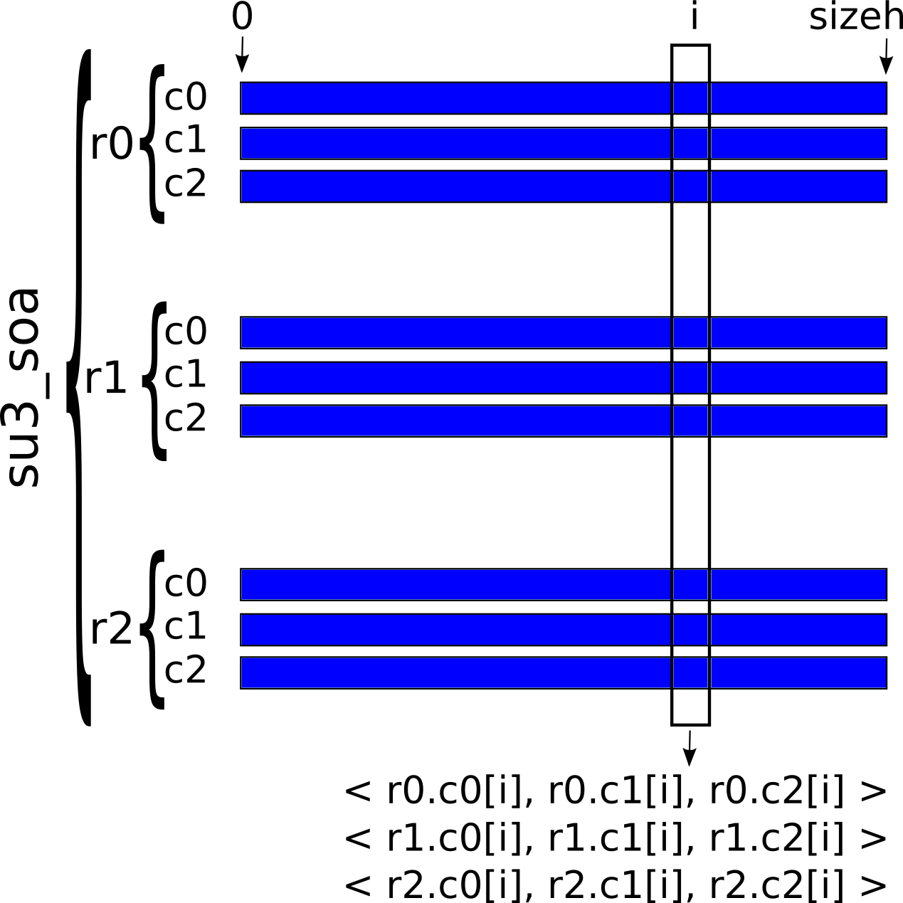
Figure 2: Memory data layout for structure su3_soa, used in the code for $SU(3)$ matrices; this structure contains 3 vectors. To mitigate memory-bandwidth requirements, one can avoid reading and writing the r2 member and recompute it on the fly, exploiting the unitarity constraint.

In our implementation, we use the C99 double complex as basic data-type which allows to use built-in complex operators of the C library making coding easier and more readable without loss of performance.

The algorithm is based on even/odd preconditioning, so the pseudo-fermion variables (implemented as vec3_soa data-types) live only on the even sites of the lattice. This comes at the price of requiring that all sides of the lattice must be even; in the following we call LNH_SIZEH half the number of lattice sites. The pseudofermion field has three complex values for each even lattice site, corresponding to the three QCD “colors” that we label c0, c1, c2. A schematic representation of the vec3_soa structure is shown in Fig. 1 and a lexicographical ordering was used for the even lattice sites:

$$\textrm{idxh}=\textrm{ \sf(int)}\frac{x_{0}+\textrm{\sf LNH\_N0}[x_{1}+\textrm{\sf LNH\_N1}(x_{2}+\textrm{\sf LNH\_N2}\,x_{3})]}{2}\qquad\mathrm{s.t.}\ \sum_{i=0}^{3}x_{i}\%2=0\ ,$$ (9)

where LNH_N0, LNH_N1 and LNH_N2 are the lattice sizes; we allow for full freedom in the mapping of the physical directions $x$, $y$, $z$ and $t$ onto the logical directions $x_{0}$, $x_{1}$, $x_{2}$ and $x_{3}$, as this option will be important for future versions of the code able to run on many processors and accelerators.

The data structure used for the generic $3\times 3$ complex matrices is the su3_soa data-type, used e.g. for the “staples” $\Sigma_{\mu}^{(k)}$ and the $\Gamma_{\mu}$ matrices needed in the stouting procedure[33]. Structure su3_soa is a collection of 3 vec3_soa structures (r0, r1, r2, see Fig. 2), and data that has to be stored in this structure typically involve a number of matrices equal to the number of links present in the lattice, i.e. 8 LNH_SIZEH; this means that an array of 8 su3_soa elements is required.

Gauge configurations, i.e. the set of the gauge links $U_{\mu}(n)$ and their stouted counterparts, are stored in memory as an array of 8 su3_soa structures. As previously explained the algorithm is typically bandwidth limited and for $SU(3)$ matrices it is convenient to read and write just the first two rows, computing the third one on the fly as ${\sf r2}=({\sf}r0\wedge{\sf r1})^{*}$. Note that the SoA memory layout avoids the prefetching problems discussed in similar cases[50].

Other data structures are needed to store in memory $3\times 3$ traceless Hermitian matrices or $3\times 3$ traceless anti-Hermitian matrices. In these cases, only 8 real parameters per matrix are needed: 3 complex numbers for the upper triangular part and the first two elements of the diagonal, which are real (imaginary) numbers for (anti-)Hermitian traceless matrices. These data structures have been implemented according to the SoA scheme as follows: thmat_soa and tamat_soa contain 3 vectors of C99 double complex numbers and 2 vectors of double numbers, in a form that closely resemble the one of vec3_soa.

Data movements between device and host are negligible, with significant transfers happening only at the beginning and at the end of each Monte Carlo update, and managed mainly with the update device and update host OpenACC directives.

4.2 Implementation methodology

To initially assess the performance level achievable using OpenACC, we have developed a mini-application benchmark of the Dirac operator[2]. As previously underlined this is the fundamental building block of the Krylov solver, commonly accounting for not less than $40\%$ of the running time, and reaching up to $80\%$ in low temperature simulations. This compute intensive part of an LQCD simulation is where most of the optimization efforts are usually concentrated[57]. The Dirac operator code uses three functions: deo, doe (corresponding respectively to the application of functions $D_{eo}$ and $D_{oe}$ defined in Eq. (7)) and a zaxpy-like function which is negligible in terms of execution time. A direct comparison indicated that the performance of the OpenACC versions of the double precision deo and doe functions were comparable with the CUDA ones[2]. This promising start was a strong indication that also for LQCD the higher portability of the OpenACC implementation is not associated with a serious loss of performance, and motivated us to proceed to an OpenACC implementation of the full RHMC code. As a side benefit, the use of the OpenACC programming model significantly simplified the implementation of algorithmic improvements.

The implementation of these new features started with the coding and testing of the improvements on a single thread version. After the algorithm is validated, the acceleration is switched on by annotating the code with #pragma directives. In order to have a more readable code, the most complex kernels have been split in several functions. While small functions can be used in kernels if declared as static inline, for larger ones we had to use the routine seq OpenACC directive as large functions cannot be inlined.

Kernels have been parallelized following two different approaches. Those using data belonging to nearest (and/or next-to-nearest) neighbors have been parallelized via the #pragma acc loop directive on $4$ nested loops, one for each dimension. This allows to use 3D thread blocks, which should improve data reuse between threads thus reducing bandwidth requirements, which is our major performance concern. The other kernels, i.e. the ones performing only single-site operations, have been parallelized using a single cycle running on the lattice sites.

Breakup of the execution time of a selection of computationally heavy steps of our OpenACC code on different architectures for low temperature and finite temperature simulations. Phase GPU NVIDIA GK201 CPU Intel E5-2630v3 Low Temp. High Temp. Low Temp. High Temp. Dirac Operator $63$ $16$ $57$ $24$ Gauge MD $8$ $56$ $1$ $24$

After the implementation of a first full working OpenACC simulation, various optimization iterations took place, in particular for the performance critical steps. These include the Dirac operator in the first place, but also the gauge part of the molecular dynamics steps, since their relative impact on the overall execution time is very large, as shown in Table 4.2 for a few representative examples.

During the full development phase, every time a new OpenACC feature has been introduced, extensive checks have been performed to ensure the correctness of the improved code, against possible semantic misunderstanding of OpenACC clauses or compiler bugs.

4.3 Implementation details of selected kernels

This section describes the overall structure of our code, and focuses on the OpenACC implementation of selected performance-critical parts.

Algorithm 1 Top level scheme of the full simulation code

1:  Read gauge configuration $U$

2:  Create momenta $p$

3:  Generate pseudofermions by heatbath

4:  Calculation of initial action

5:  Molecular Dynamics [possibly in single precision]

6:  Calculate action variation $\Delta S$

7:  Montecarlo step accepted with probability $\textrm{min}(1,e^{-\Delta S})$

8:  Take measurements

Algorithm 1 is a top-level description of the full code, showing the main computational tasks. For performances, the most critical steps are Molecular Dynamics (step 5) followed by the heatbath generation of the pseudofermions (step 3), and the calculation of the final action (step 6). Steps 3 and 6 consist basically in function calls to the multishift inverter routine, with a high target accuracy.

The outer level of the multistep integrator for Molecular Dynamic evolution (step 5) in Algorithm 1 is expanded in Algorithm 2. As explained in Sec.(2.1), in zero temperature simulations or for small quark masses usually the heaviest computational parts are the calculations of the fermion force, while in high temperature simulations the load is shifted inside the gauge cycles, as already shown in Table 4.2. The fermion force calculation step is implemented following[33]; for this step a large fraction of the execution time is is spent in computation of deo and doe functions implementing the Dirac operator.

Listing 2: OpenACC implementation of the Deo function; directive vector tile divides the computational domain in sub-lattices (tiles), each processed within a compute unit in order to allow data re-use.

⬇

void acc_Deo( __restrict const su3_soa * const u,

__restrict vec3_soa * const out,

__restrict const vec3_soa * const in,

__restrict const double_soa * const backfield){

int hd0, d1, d2, d3;

#pragma acc kernels present(in) present(out)

present(u) present(backfield) async(1)

#pragma acc loop independent gang(GANG)

for(d3=0; d3<nd3;d3++) {

#pragma acc loop independent vector tile(TILE0,TILE1,TILE2)

for(d2=0; d2<nd2; d2++) {

for(d1=0; d1<nd1; d1++) {

for(hd0=0; hd0 < nd0h; hd0++) {

...

}

}

}

}

}

The deo OpenACC implementation is shown in Listing 2, showing the 4 dimension nested loops and the corresponding pragma directives. In this listing OpenACC directives are used: i) to identify the data structures already present in the accelerator memory, when targeting accelerators (present() clause); ii) to make the compiler aware of the data independence of loops iterations (independent clause); iii) to request to group iterations in order to execute them in the same (or close) compute units (tile clause). In particular, the tile OpenACC clause asks the compiler to split or strip-mine each loop in the nest into two loops, an outer tile loop and an inner element loop.

Where possible (e.g. in deo and doe), performing computations of adjacent lattice sites in close hardware compute units may increase data reuse (i.e. matrices shared between sites)[57] for all the architectures where data caches are present, which means almost every modern processing architecture. The tile sizes offering the best performance depend, for each kernel, on several features of each specific architecture, e.g. vector units size, register numbers, cache levels and sizes. We keep a door open for limited architecture-specific optimization, by allowing to specify the TILE0, TILE1, TILE2 variables at compile time, telling the compiler how to group together iterations involving adjacent lattice sites.

Algorithm 2 MD evolution - 2nd order Minimum Norm integrator (outer cycle)

1:  Fermion Force Calculation

2:  Evolve momenta for $\lambda\Delta T/N_{md}$                                 {$\lambda=0.1931833275037836$}[46]

3:  for $i=1$ to $N_{md}-1$ do

4:     Gauge cycle ($\Delta T/2N_{md}$)

5:     Fermion Force Calculation

6:     Evolve momenta for $(1-2\lambda)\Delta T/N_{md}$

7:     Gauge cycle ($\Delta T/2N_{md}$)

8:     Fermion Force Calculation

9:     Evolve momenta for $2\lambda\Delta T/N_{md}$

10:  end for

11:  Gauge cycle ($\Delta T/2N_{md}$)

12:  Fermion Force Calculation

13:  Evolve momenta for $(1-2\lambda)\Delta T/N_{md}$

14:  Gauge cycle ($\Delta T/2N_{md}$)

15:  Fermion Force Calculation

16:  Evolve momenta for $\lambda\Delta T/2N_{md}$

The actual evolution of the gauge configuration happens inside the inner gauge cycles, where the gauge contribution to the momenta evolution is also calculated. Among the tasks performed in the gauge cycles, the computation of staples in the gauge force calculation is the most time consuming. It consists of calculating 6 products of 3 and 5 $SU(3)$ matrices representing links on C-shaped paths on the lattice.

The implementation of one of these functions is sketched in Listing 3: also in this case the parallelization has been done using the tile directive over the 3 innermost nested cycles. This allows us also in this case to use 3D thread blocks, which should improve data reuse between threads, reducing the bandwidth needs. We shall also remark that in this case, since second-nearest-neighbor-site addressing is needed, for the sake of simplicity we use indirect addressing. Notice that the function staple_type1 (as well as similar ones) has to be declared with #pragma acc routine seq to be used inside a kernel.

Listing 3: Implementation of the function performing the evaluation of a staple.

⬇

#pragma acc routine seq

void staple_type1(...){...}

void calc_staples_type1( __restrict const su3_soa * const u,

__restrict su3_soa * const loc_stap ) {

int d0, d1, d2, d3, mu, iter;

#pragma acc kernels present(u) present(loc_stap)

present(nnp_openacc) present(nnm_openacc)

#pragma acc loop independent gang(IMPSTAPGANG3)

for(d3=0; d3<nd3; d3++){

#pragma acc loop independent vector tile(IMPSTAPTILE0,

IMPSTAPTILE1,

IMPSTAPTILE2)

for(d2=0; d2<nd2; d2++) {

for(d1=0; d1<nd1; d1++) {

for(d0=0; d0 < nd0; d0++) {

#pragma acc loop seq

for(mu=0; mu<4; mu++){

...

const int idx_pmu = nnp_openacc[idxh][mu][parity];

...

staple_type1(&u[dir_nu_1R], idx_pmu, ... )

In order to improve performance, we also implemented a single precision version of the code for the molecular dynamics evolution. Due to the low arithmetic density of the LQCD algorithms, on GPUs at least, all kernels are memory-bound; this means that, when precision is not an issue, it is preferable to have single precision versions of selected functions and structures, as a plain $\times 2$ increase in performance is expected with respect to the double precision implementation.

5 Performance analysis

To compare the performance of our code on different architectures we consider two different benchmarks taking into account the most computational intensive parts of the code. The first benchmark evaluates the performance of the Dirac operator, both single and double precision version, and the latter evaluates the performance of the gauge part of the molecular dynamics step. Depending on input configuration parameters either the former or the latter kernels make up most of the execution time of a typical simulation, as shown in Table 4.2.

We present the execution time per site of the Dirac operator for different lattice sizes in Table 5. Exactly the same code has been run on all platforms without requiring any change; we have just re-compiled it with different flags instructing the PGI 16.10 compiler to target the corresponding architectures and using the best tile dimensions for each of them.

Measured execution time per lattice site [ns] for the Dirac operator, on several processors and for several typical lattice sizes. Lattice Processor (CPU or GPU) NVIDIA GK201 NVIDIA P100 Intel E5-2630v3 Intel E5-2697v4 SP DP SP DP SP DP SP DP $32^{2}\times 8\times 32$ $4.19$ $8.51$ $1.77$ $3.07$ $72.18$ $99.17$ $38.92$ $54.90$ $32^{3}\times 8$ $4.15$ $8.39$ $1.22$ $2.48$ $72.81$ $101.46$ $77.33$ $103.87$ $24^{4}$ $4.43$ $8.62$ $1.58$ $2.90$ $70.44$ $94.42$ $51.13$ $66.87$ $32^{4}$ $4.02$ $9.54$ $1.32$ $2.40$ $79.05$ $100.19$ $43.90$ $54.88$ $32^{3}\times 36$ $4.03$ $8.48$ $1.46$ $2.54$ $83.12$ $107.47$ $38.82$ $50.29$

We tested two different NVIDIA GPUs, the K80 based on the Kepler architecture and the recently released P100 board based on the Pascal architecture. For the K80 the single precision version takes $\approx 4ns$ per lattice site, while the double precision version requires $\approx 8.5ns$. Running on the P100 we measure $\approx 1.5ns$ for single and $\approx 2.5ns$ for double precision, improving approximately by a factor $3\times$ over the K80. This results perfectly scales with architecture performance of P100 that has $\approx 4.3\times$ more cores and $\approx 3\times$ more memory bandwidth, see Table 3.

Concerning Intel CPUs, we have compared two different processors, the 8-core E5-2630v3 CPU based on Haswell architecture, and the 18-core E5-2697v4 CPU based on Broadwell. Since computing resource of the CPUs are roughly $3\times$ lower than on GPUs, see Table 3, a performance drop is expected. However, the actual performance drop measured on both CPUs is much larger than this expected theoretical figure; indeed time per site is approximately $10\times$ or larger on the Haswell than on one K80 GPU. The Broadwell performs approximately a factor $2\times$ better compared to Haswell, at least for some lattice sizes. We have identified two main reasons for this non-optimal behavior, and both of them point to some still immature features of the PGI compiler when targeting x86 architectures, that – we expect – should be soon resolved:

• Parallelization - the compiler is only able to split outer-loops across different threads, while inner loops are executed serially or vectorized within each thread. This explains why on the Broadwell CPU running on a lattice $32^{2}\times 8\times 32$ we have a performance $2\times$ better than for a $32^{3}\times 8$ lattice, which has the same volume but allows to split the outer loop only on $8$ threads.

• Vectorization - as reported by the compilation logs, the compiler fails to vectorize the deo and doe functions computing the Dirac operator (see Listing 2) reporting to be unable to vectorize due to the use of “mixed data-types”. To verify if this is related to how we have coded these functions, we have translated the OpenACC pragmas into the corresponding OpenMP ones – without changing the C code – and compiled using the Intel compiler (version 17.0.1). In this case the compiler succeeds in vectorizing the two functions, running a factor $2\times$ faster compared to the OpenACC version compiled by PGI compiler.

Measured execution time per lattice site [ns] for the pure gauge Molecular Dynamics step for several processors and several typical lattice sizes. Lattice Processor (CPU or GPU) NVIDIA GK201 NVIDIA P100 Intel E5-2630v3 Intel E5-2697v4 $32^{2}\times 8\times 32$ $193.79$ $51.80$ $1613.88$ $926.48$ $32^{3}\times 8$ $190.39$ $51.69$ $2075.08$ $1756.78$ $24^{4}$ $212.04$ $53.74$ $1265.13$ $979.28$ $32^{4}$ $201.82$ $51.72$ $1719.97$ $944.40$ $32^{3}\times 36$ $208.54$ $52.62$ $1801.81$ $837.68$

Table 5 shows the execution time of the gauge part of the molecular dynamics step. As already remarked this is one of the two most time-consuming steps together with the application of the Dirac operator. As we see the update time per site is quite stable for all lattice sizes we have tried and for all architectures. Going from the NVIDIA K80 to the P100 the time improves by a factor $\approx 3\times$, while between Haswell and Broadwell we have roughly a factor $\approx 1.5\times$ / $2.0\times$.

We finally mention that we have also been able to compile and run our code on an AMD FirePro W9100 GPU and on the latest version of the Intel Xeon Phi processor, the Knights Landing (KNL). However, in these cases, results are still preliminary. In more details, the compiler itself crashes when compiling the code for the AMD GPU for some specific lattice sizes; for the KNL, specific compiler support is still missing, but this processor is able to run the code compiled for the Haswell architecture, implying however that 512-bit vectorization is not used. These problems do not allow us to perform a systematic comparison of performance for these architectures. Once again, we believe that this is due to some immaturity of the compiler, and we expect that these issues will be resolved in future versions.

Execution time [sec] of a full trajectory of a complete Monte Carlo simulation for several typical physical parameters, running on one GPU of a NVIDIA K80 system. We compare the OpenACC code developed in this paper and and earlier GPU-optimized CUDA code. Here we use the standard Wilson action and unimproved staggered fermions as the CUDA code does not support the more advanced improvements available in the OpenACC version. Lattice $am$ $\beta$ CUDA OpenAcc Variation $32^{3}\times 8$ $0.0125$ $5.55$ $392.69$ $490.74$ +25% $24^{4}$ $0.0125$ $5.55$ $303.80$ $328.07$ +8% $32^{4}$ $0.001$ $5.52$ $8973.82$ $8228.36$ -8%

Table 5 addresses the question of the efficiency costs (if any) of our architecture-portable code; the table compares the execution time for a full Monte Carlo step (in double precision) of the OpenACC code and a previously developed CUDA implementation[21], optimized for NVIDIA GPUs. Although the two codes are not exactly in a one to one correspondence, the implementations are similar enough to make such a test quantitatively meaningful. One immediately sees that the performances of the two implementations are comparable and the use of OpenACC does not imply a dramatic performance loss, the differences between the execution times of the two versions being of the order of $10\div 20\%$.

The worst case is the one of the $32^{3}\times 8$ lattice, in which OpenACC is about $25\%$ slower than CUDA. Since we are comparing an high-level version of the code with one specifically developed for NVIDIA GPUs, this would not be a dramatic loss, however in this case the comparison is also not completely fair. Indeed for this high temperature simulation the gauge part of the Molecular Dynamic step starts to be the computationally heaviest task and, in the CUDA implementation, part of it had been explicitly hard coded in single precision.

For the low-temperature test cases the differences between the CUDA and the OpenACC implementation are much smaller and, in fact, in one case the OpenACC version is the fastest one. A possible explanation of this is the following: in the CUDA version unidimensional blocks are adopted to parallelize the Dirac operator, while in the OpenACC implementation three-dimensional block structures are used, that fit better the larger cache of recent GPUs and, especially on larger lattices, improves data reuse.

6 Concluding Remarks

In this work we have developed a full state-of-the-art production-grade code for Lattice QCD simulations with staggered fermions, using the OpenACC directive-based programming model. Our implementation includes all steps of a complete simulation, and most of them run on accelerators, minimizing the transfer of lattice data to and from the host. We have used the PGI compiler, which supports the OpenACC standard and is able to target almost all current architectures relevant for HPC computing, even if with widely different levels of maturity and reliability. Exactly the same code runs successfully on NVIDIA many-core GPUs and Intel multi-core CPUs, and for both architectures we have measured roughly comparable levels of efficiency. Also, the performance of the complete code is roughly the same as that of an equivalent code, specifically optimized for NVIDIA GPUs and written in the CUDA language. Our code also runs on AMD GPUs and on the KNL Intel Phi processor, even if the compilation and run-time environment for these processors is still unable to deliver production-grade codes; in these cases, we have strong indications that these problems come from a residual immaturity of the compilation chain and we expect that they will be soon resolved. All in all, our final result is a LQCD Monte Carlo code portable on a large subset of HPC relevant processor architectures and with consistent performances.

Some further comments are in order: i) using a directive-based programming model, we are able to target different computing platforms presently used for HPC, avoiding to rewrite the code when moving from one platform to another; ii) the OpenACC standard provides a good level of hardware abstraction requiring the programmer to only specify the function to be parallelized and executed on the accelerator; the compiler is then able to exploit the parallelism according to the target processor, hiding from the programmer most hardware optimizations; iii) the OpenACC code has roughly the same level of performance of that implemented using a native language such as CUDA for NVIDIA GPUs, allowing to efficiently exploit the computing resources of the target processor.

In the near future we plan to carefully assess performances on AMD and KNL systems, in order to enlarge the platform portfolio of our code. We also plan to assess whether OpenMP4 provides the same level of portability as OpenACC, as soon as compilers supporting this programming standard become available. This is important to have a unique directive-based programming model which is widely used by several scientific communities and supported by several compilers (GCC, ICC, …). Finally, we are already working on a massively parallel version of our code, able to run concurrently on a large clusters of CPUs and accelerators.

References

- [1] O. Villa, D. R. Johnson, M. O’Connor, E. Bolotin, D. Nellans, J. Luitjens, N. Sakharnykh, P. Wang, P. Micikevicius, A. Scudiero, S. W. Keckler and W. J. Dally, Scaling the power wall: A path to exascale, in Proceedings of the International Conference for High Performance Computing, Networking, Storage and Analysis, SC ’14 (IEEE Press, Piscataway, NJ, USA, 2014). doi:10.1109/SC.2014.73.
- [2] C. Bonati, E. Calore, S. Coscetti, M. D’Elia, M. Mesiti, F. Negro, S. F. Schifano and R. Tripiccione, Development of scientific software for HPC architectures using OpenACC: the case of LQCD, in The 2015 International Workshop on Software Engineering for High Performance Computing in Science (SE4HPCS), ICSE Companion Proceedings2015. doi:10.1109/SE4HPCS.2015.9.
- [3] D. Pflüger, M. Mehl, J. Valentin, F. Lindner, D. Pfander, S. Wagner, D. Graziotin and Y. Wang, The scalability-efficiency/maintainability-portability trade-off in simulation software engineering: Examples and a preliminary systematic literature review, in Proceedings of the Fourth International Workshop on Software Engineering for HPC in Computational Science and Engineering, SE-HPCCSE ’162016. doi:10.1109/SE-HPCCSE.2016.8.
- [4] The OpenMP API specification for parallel programming.
- [5] OpenACC directives for accelerators.
- [6] S. Wienke, C. Terboven, J. Beyer and M. Müller, Lecture Notes in Computer Science (including subseries Lecture Notes in Artificial Intelligence and Lecture Notes in Bioinformatics) 8632, 812 (2014).
- [7] M. G. Lopez, V. V. Larrea, W. Joubert, O. Hernandez, A. Haidar, S. Tomov and J. Dongarra, Towards achieving performance portability using directives for accelerators, in Proceedings of the Third International Workshop on Accelerator Programming Using Directives, WACCPD ’162016. doi:10.1109/WACCPD.2016.9.
- [8] The Portland Group, Inc. http://www.pgroup.com/
- [9] C. Bernard et al., Nucl. Phys. Proc. Suppl. 106, 199 (2002).
- [10] G. Bilardi, A. Pietracaprina, G. Pucci, F. Schifano and R. Tripiccione, Lecture Notes in Computer Science 3769, 386 (2005), doi:10.1007/11602569_41.
- [11] M. Albanese et al., Comput. Phys. Commun. 45, 345 (1987), doi:10.1016/0010-4655(87)90172-X.
- [12] F. Belletti, S. F. Schifano, R. Tripiccione, F. Bodin, P. Boucaud, J. Micheli, O. Pene, N. Cabibbo, S. De Luca, A. Lonardo, D. Rossetti, P. Vicini, M. Lukyanov, L. Morin, N. Paschedag, H. Simma, V. Morenas, D. Pleiter and F. Rapuano, Computing in Science and Engineering 8, 50 (2006), doi:10.1109/MCSE.2006.4.
- [13] P. A. Boyle, D. Chen, N. H. Christ, M. Clark, S. Cohen, Z. Dong, A. Gara, B. Joo, C. Jung, L. Levkova, X. Liao, G. Liu, R. D. Mawhinney, S. Ohta, K. Petrov, T. Wettig, A. Yamaguchi and C. Cristian, Qcdoc: A 10 teraflops computer for tightly-coupled calculations, in Supercomputing, 2004. Proceedings of the ACM/IEEE SC2004 Conference, Nov 2004. doi:10.1109/SC.2004.46.
- [14] H. Baier, H. Boettiger, M. Drochner, N. Eicker, U. Fischer, Z. Fodor, A. Frommer, C. Gomez, G. Goldrian, S. Heybrock, D. Hierl, M. Hüsken, T. Huth, B. Krill, J. Lauritsen, T. Lippert, T. Maurer, B. Mendl, N. Meyer, A. Nobile, I. Ouda, M. Pivanti, D. Pleiter, M. Ries, A. Schäfer, H. Schick, F. Schifano, H. Simma, S. Solbrig, T. Streuer, K.-H. Sulanke, R. Tripiccione, J.-S. Vogt, T. Wettig and F. Winter, Computer Science - Research and Development 25, 149 (2010), doi:10.1007/s00450-010-0122-4.
- [15] J. Doi, Peta-scale lattice quantum chromodynamics on a blue gene/q supercomputer, in Proceedings of the International Conference on High Performance Computing, Networking, Storage and Analysis, SC ’12 (IEEE Computer Society Press, Los Alamitos, CA, USA, 2012).
- [16] G. I. Egri, Z. Fodor, C. Hoelbling, S. D. Katz, D. Nogradi and K. K. Szabo, Comput. Phys. Commun. 177, 631 (2007), doi:10.1016/j.cpc.2007.06.005.
- [17] K. Barros, R. Babich, R. Brower, M. A. Clark and C. Rebbi, PoS LATTICE 2008, 045 (2008) [arXiv:0810.5365 [hep-lat]].
- [18] R. Babich, M. A. Clark and B. Joo, Parallelizing the QUDA Library for Multi-GPU Calculations in Lattice Quantum Chromodynamics, in SC 10 (Supercomputing 2010) New Orleans, Louisiana, November 13-19, 2010, 2010.
- [19] N. Cardoso and P. Bicudo, J. Comput. Phys. 230, 3998 (2011) [arXiv:1010.4834 [hep-lat]] doi:10.1016/j.jcp.2011.02.023.
- [20] T. W. Chiu et al. [TWQCD Collaboration], Phys. Lett. B 702, 131 (2011) [arXiv:1105.4414 [hep-lat]] doi:10.1016/j.physletb.2011.06.070.
- [21] C. Bonati, G. Cossu, M. D’Elia and P. Incardona, Computer Physics Communications 183, 853 (2012), doi:10.1016/j.cpc.2011.12.011.
- [22] M. Bach, V. Lindenstruth, O. Philipsen and C. Pinke, Comput. Phys. Commun. 184, 2042 (2013), doi:10.1016/j.cpc.2013.03.020.
- [23] O. Philipsen, C. Pinke, A. Sciarra and M. Bach, CLQCD - Lattice QCD based on OpenCL, in Proceedings, GPU Computing in High-Energy Physics (GPUHEP2014): Pisa, Italy, September 10-12, 2014, 2015. doi:10.3204/DESY-PROC-2014-05/30.
- [24] S. Blair, C. Albing, A. Grund and A. Jocksch, Accelerating an mpi lattice boltzmann code using openacc, in Proceedings of the Second Workshop on Accelerator Programming Using Directives, WACCPD ’15 (ACM, New York, NY, USA, 2015). doi:10.1145/2832105.2832111.
- [25] J. Kraus, M. Schlottke, A. Adinetz and D. Pleiter, Accelerating a c++ cfd code with openacc, in Accelerator Programming using Directives (WACCPD), 2014 First Workshop on, 2014. doi:10.1109/WACCPD.2014.11.
- [26] E. Calore, A. Gabbana, J. Kraus, S. F. Schifano and R. Tripiccione, Concurrency and Computation: Practice and Experience 28, 3485 (2016), doi:10.1002/cpe.3862.
- [27] P. Majumdar, Journal of Physics: Conference Series 759, p. 012070 (2016).
- [28] C. Patrignani, P. D. Group et al., Chinese physics C 40, p. 100001 (2016).
- [29] K. G. Wilson, Physical Review D 10, p. 2445 (1974).
- [30] D. Weingarten and D. Petcher, Physics Letters B 99, 333 (1981).
- [31] P. Weisz, Nuclear Physics B 212, 1 (1983).
- [32] G. Curci, P. Menotti and G. Paffuti, Physics Letters B 130, 205 (1983).
- [33] C. Morningstar and M. Peardon, Physical Review D 69, p. 054501 (2004).
- [34] S. Duane, A. D. Kennedy, B. J. Pendleton and D. Roweth, Physics letters B 195, 216 (1987).
- [35] A. Kennedy, arXiv preprint hep-lat/0607038 (2006).
- [36] M. Clark, A. Kennedy and Z. Sroczynski, arXiv preprint hep-lat/0409133 (2004).
- [37] M. Clark and A. Kennedy, Physical review letters 98, p. 051601 (2007).
- [38] M. Clark and A. Kennedy, Physical Review D 75, p. 011502 (2007).
- [39] B. Jegerlehner, arXiv preprint hep-lat/9612014 (1996).
- [40] V. Simoncini and D. B. Szyld, Numerical Linear Algebra with Applications 14, 1 (2007).
- [41] T. DeGrand and C. DeTar, Lattice methods for quantum chromodynamics (World Scientific, 2006).
- [42] T. A. Degrand and P. Rossi, Computer Physics Communications 60, 211 (1990), doi:http://dx.doi.org/10.1016/0010-4655(90)90006-M.
- [43] J. Sexton and D. Weingarten, Nuclear Physics B 380, 665 (1992).
- [44] C. Urbach, K. Jansen, A. Shindler and U. Wenger, Computer Physics Communications 174, 87 (2006).
- [45] I. Omelyan, I. Mryglod and R. Folk, Physical Review E 65, p. 056706 (2002).
- [46] I. Omelyan, I. Mryglod and R. Folk, Computer Physics Communications 151, 272 (2003).
- [47] T. Takaishi and P. De Forcrand, Physical Review E 73, p. 036706 (2006).
- [48] P. De Forcrand, D. Lellouch and C. Roiesnel, Journal of Computational Physics 59, 324 (1985).
- [49] M. A. Clark, R. Babich, K. Barros, R. C. Brower and C. Rebbi, Computer Physics Communications 181, 1517 (2010).
- [50] B. Joó, M. Smelyanskiy, D. D. Kalamkar and K. Vaidyanathan, Wilson dslash kernel from lattice QCD optimization, in High Performance Parallelism Pearls Volume 2: Multicore and Many-core Programming Approaches, eds. J. Reinders and J. Jeffers (Morgan Kaufmann, Boston, 2015), pp. 139–170. doi:10.1016/B978-0-12-803819-2.00023-9.
- [51] NVIDIA’s Next Generation CUDA™ Compute Architecture: Kepler™ GK110/210 (2014).
- [52] NVIDIA Tesla P100 v1.1 (2016).
- [53] The Radeon R9 290x Review.
- [54] Intel’s Haswell CPU Microarchitecture.
- [55] F. Sanfilippo. https://github.com/sunpho84/nissa/.
- [56] E. Calore, N. Demo, S. F. Schifano and R. Tripiccione, Experience on vectorizing lattice boltzmann kernels for multi- and many-core architectures, in Parallel Processing and Applied Mathematics: 11th International Conference, PPAM 2015, Krakow, Poland, September 6-9, 2015. Revised Selected Papers, Part I, eds. R. Wyrzykowski, E. Deelman, J. Dongarra, K. Karczewski, J. Kitowski and K. WiatrLecture Notes in Computer Science (Springer International Publishing, Cham, 2016), pp. 53–62. doi:10.1007/978-3-319-32149-3_6.
- [57] B. Joó, M. Smelyanskiy, D. D. Kalamkar and K. Vaidyanathan, Chapter 9 - wilson dslash kernel from lattice QCD optimization, in High Performance Parallelism Pearls, eds. J. Reinders and J. Jeffers (Morgan Kaufmann, 2015), pp. 139 – 170. doi:10.1016/B978-0-12-803819-2.00023-9.
- [58] B. Joó, D. D. Kalamkar, T. Kurth, K. Vaidyanathan and A. Walden, Optimizing Wilson-Dirac Operator and Linear Solvers for Intel KNL, in High Performance Computing: ISC High Performance 2016 International Workshops, eds. M. Taufer, B. Mohr and J. M. Kunkel (Springer International Publishing, June 2016), pp. 415–427. Revised Selected Papers.