Heavy-quark meson spectrum tests of the Oktay-Kronfeld action

Abstract

The Oktay-Kronfeld (OK) action extends the Fermilab improvement program for massive Wilson fermions to higher order in suitable power-counting schemes. It includes dimension-six and -seven operators necessary for matching to QCD through order $\mathrm{O}(\Lambda^{3}/m_{Q}^{3})$ in HQET power counting, for applications to heavy-light systems, and $\mathrm{O}(v^{6})$ in NRQCD power counting, for applications to quarkonia. In the Symanzik power counting of lattice gauge theory near the continuum limit, the OK action includes all $\mathrm{O}(a^{2})$ and some $\mathrm{O}(a^{3})$ terms. To assess whether the theoretical improvement is realized in practice, we study combinations of heavy-strange and quarkonia masses and mass splittings, designed to isolate heavy-quark discretization effects. We find that, with one exception, the results obtained with the tree-level-matched OK action are significantly closer to the continuum limit than the results obtained with the Fermilab action. The exception is the hyperfine splitting of the bottom-strange system, for which our statistical errors are too large to draw a firm conclusion. These studies are carried out with data generated with the tadpole-improved Fermilab and OK actions on 500 gauge configurations from one of MILC’s $a\approx 0.12$ fm, $N_{f}=2+1$-flavor, asqtad-staggered ensembles.

I Introduction

Lattice QCD has been used to calculate nonperturbatively hadronic matrix elements needed for many aspects of Standard Model (SM) phenomenology. For example, hadronic matrix elements of flavor-changing currents are crucial to quark-flavor physics (see, e.g., Ref. Du et al. (2016)), and many of them are gold-plated calculations Davies et al. (2004) in lattice QCD. For gold-plated light-quark processes, lattice QCD has achieved high precision Aoki et al. (2016). Especially notable is the hadronic matrix element $B_{K}$ needed to understand indirect CP violation in the neutral kaon system, which is known to 1.3% Dürr et al. (2011); Laiho and Van de Water (2011); Blum et al. (2016); Carrasco et al. (2015); Choi et al. (2016); Aoki et al. (2016). That said, simulating heavy quarks in lattice QCD is a long-standing challenge Kronfeld (2004); El-Khadra (2014); Bouchard (2015), and in this paper we examine a way to control discretization effects for massive (i.e., $m_{Q}\gg\Lambda$) fermions in lattice gauge theory El-Khadra et al. (1997); Kronfeld (2000); Oktay and Kronfeld (2008); Burch et al. (2010).

In the SM, the Cabibbo-Kobayashi-Maskawa (CKM) matrix explains all changes of quark flavor. The CKM matrix contains four independent parameters, three angles and one phase, with the phase being responsible for CP violation. Three of the four parameters are the magnitude and phase of the matrix element $V_{ub}$ and the magnitude of $V_{cb}$. In practice, $|V_{cb}|$, $|V_{ub}|$, and $\arg V_{ub}$ are determined in $B$-meson decays and CP asymmetries. The remaining CKM parameter is the Cabibbo angle, i.e., $|V_{us}|$, which is known from kaon decays to 0.3% Bazavov et al. (2014a, b); Patrignani et al. (2016).

In $B$ physics, the unitarity of the CKM matrix is often visualized with the unitarity triangle (UT). Indirect CP violation in the neutral kaon system constrains the apex of the UT via the quantity $\varepsilon_{K}$. In the SM, $\varepsilon_{K}$ depends parametrically on $|V_{cb}|$ to the fourth power. There is a $3.2\sigma$ tension between $\varepsilon_{K}$ in the SM Bailey et al. (2016a); Lee (2016); Bailey et al. (2015a) and experiment Ambrosino et al. (2006) when the exclusive value of $|V_{cb}|$ DeTar (2016) from the decays $\bar{B}\to D^{(*)}\ell\bar{\nu}$ is taken as input. In contrast with the 0.5% uncertainty in the experimental value of $\varepsilon_{K}$, there is a 10% uncertainty in this SM prediction, mostly coming from an uncertainty in the CKM matrix element $|V_{cb}|$.

In addition, there is a $3\sigma$ tension between the exclusive Bailey et al. (2014a) and inclusive Alberti et al. (2015) determinations of $|V_{cb}|$, and a similar tension of 2–3$\sigma$ in $|V_{ub}|$ Ricciardi (2016, 2013). Therefore, to conduct stringent tests of the SM description of flavor physics, reducing the errors of $|V_{ub}|$ and $|V_{cb}|$ is necessary. At present, the experimental and theoretical errors on $|V_{ub}|$ and $|V_{cb}|$ are comparable. The target is promising because the experimental precision of the decay rates will get better with the Belle II and LHCb experiments. On the theoretical side, the errors in the form factors of the semileptonic decays, $\bar{B}\to D^{(*)}\ell\bar{\nu}$, for $|V_{cb}|$, and $\bar{B}\to\pi\ell\bar{\nu}$, for $|V_{ub}|$, must be reduced.

Another interesting quantity is the $B_{(s)}$-meson decay constant, $f_{B_{(s)}}$. Its physical significance is highlighted in the rare leptonic decay $B_{s}\to\mu^{+}\mu^{-}$. This decay is sensitive to new physics, because, as a flavor-changing neutral-current process, it is a suppressed, higher-order loop-effect in the SM. Thus, the decay $B_{s}\to\mu^{+}\mu^{-}$ can place strong constraints on beyond the SM models El-Khadra (2014); Horgan et al. (2014, 2015). Currently, many lattice-QCD collaborations have calculated the decay constant $f_{B_{(s)}}$ Bazavov et al. (2012); McNeile et al. (2012); Na et al. (2012); Dowdall et al. (2013); Christ et al. (2015), and the results are consistent within errors Aoki et al. (2016). Increasing the precision of the lattice-QCD determination will provide stronger constraints.

A major challenge in increasing the precision of lattice QCD calculations of heavy-quark quantities is to control heavy-quark discretization errors. Because the heavy-quark, $b$ and $c$, masses and the accessible ultraviolet cutoff $a^{-1}$ are comparable, special care is needed to handle heavy quark discretization effects. Following the development of nonrelativistic QED for the study of bound states Caswell and Lepage (1986), nonrelativistic QCD (NRQCD) was developed for lattice calculations of hadronic bound states Lepage and Thacker (1988); Thacker and Lepage (1991); Davies and Thacker (1992); Lepage et al. (1992) and quarkonium phenomenology Bodwin et al. (1995). A similar approach, heavy quark effective theory (HQET), was adopted for lattice calculations of heavy-light systems, treating heavy quarks as a static chromoelectric source Eichten (1988); Eichten and Hill (1990a, b).

Whereas NRQCD and HQET are nonrelativistic effective field theories treating heavy quarks as two-component spinors, the Fermilab action El-Khadra et al. (1997) is based on the Wilson clover action Wilson (1977); Sheikholeslami and Wohlert (1985) with four-component spinors. To retain a suitable remnant of Lorentz symmetry in physical quantities, the lattice action must have a time-space axis-interchange asymmetric form. The Fermilab action is then tuned with explicitly (bare) mass dependent couplings $c_{i}(m_{0}a)$ to connect smoothly the large $m_{Q}a>1$ and small $m_{Q}a\ll 1$ mass limits. In this way, the discretization errors can be controlled for arbitrary quark mass. In addition, a continuum limit without fine tuning is possible with the Fermilab action, which is not the case with direct discretizations of NRQCD.

The Fermilab action is applicable to both heavy-light systems and quarkonia, with suitable power counting: HQET power counting Kronfeld (2000); Oktay and Kronfeld (2008) for heavy-light systems and NRQCD for quarkonia Lepage et al. (1992); Oktay and Kronfeld (2008); Burch et al. (2010). Using ideas from the effective theories, one can develop a HQET- or NRQCD-based theory of cutoff effects El-Khadra et al. (1997); Kronfeld (2000); Oktay and Kronfeld (2008); Burch et al. (2010), yielding a systematic improvement and error estimation method. This nonrelativistic analysis establishes a different interpretation, in which one tuning condition is not imposed, without introducing large discretization effects into matrix elements and mass splittings. This technique, often known as the Fermilab nonrelativistic interpretation, is used in the heavy-quark calculations of the Fermilab Lattice and MILC Collaborations. Related approaches Aoki et al. (2003); Christ et al. (2007) essentially use the Fermilab action, but impose the tuning condition left out in the Fermilab nonrelativistic interpretation.

The Oktay-Kronfeld (OK) action Oktay and Kronfeld (2008) is an extension of the Fermilab action that incorporates all dimension-six and certain dimension-seven bilinear operators. Although there are many such operators, many can be eliminated as redundant. Furthermore, only six are needed for tree-level matching to QCD through $\mathrm{O}(\lambda^{3})$ ($\lambda\sim\Lambda_{\text{QCD}}/m_{Q}$ or $\Lambda_{\text{QCD}}a$) in HQET power counting for heavy-light mesons and $\mathrm{O}(v^{6})$ ($v$ being the relative velocity of the quark and antiquark) in NRQCD power counting for quarkonium. When $m_{0}a\ll 1$, OK improvement reduces to $\mathrm{O}(a^{2})$ with some $\mathrm{O}(a^{3})$ terms in Symanzik Symanzik (1983) power counting. It is expected that the bottom- and charm-quark discretization errors could be reduced below the $1\%$ level with the OK action Oktay and Kronfeld (2008). A similar error can be achieved with other highly improved actions, such as highly-improved staggered quarks Follana et al. (2007), once the lattice spacing is small enough.

To test whether the theoretical improvement Oktay and Kronfeld (2008) is achieved in practice, we form combinations of heavy-light meson and quarkonium masses, designed to isolate discretization errors. For spin-independent improvements, we compute a combination of heavy-light and quarkonium masses discussed in Refs. Collins et al. (1996); Kronfeld (1997). For spin-dependent improvements, we compute the hyperfine splittings in each system. For the work reported here, we generate data using a MILC asqtad-staggered $N_{f}=2+1$ ensemble with $a\approx 0.12$ fm Bazavov et al. (2010). We use an optimized conjugate gradient inverter Jang et al. (2014) to calculate quark propagators with both the tadpole-improved Fermilab and OK actions over ranges spanning the $b$ and $c$ quarks. For the $b$-like and $c$-like quarks, the data are generated with four different values of the hopping parameter for the OK action, and two for the Fermilab action. Tadpole improvement of all terms is fully implemented in the conjugate-gradient program, as in an early, preliminary study DeTar et al. (2010). A preliminary report of the analysis reported here can be found in Ref. Bailey et al. (2014b).

The outline of this paper is as follows. In Sec. II, we briefly review the OK action and discuss its tadpole improvement. In Sec. III, we describe the correlators we generate and the fits we use to extract the lightest meson energies in each channel at each momentum. In Sec. IV, we describe the fits needed to extract the rest and kinetic masses of the pseudoscalar and vector mesons. In Sec. V, we assess the improvement from higher-order kinetic terms in the OK action with the mass combination of Refs. Collins et al. (1996); Kronfeld (1997). In Sec. VI, we assess the improvement from higher-order chromomagnetic interactions in the OK action by inspecting the difference of the hyperfine splittings of the rest and kinetic masses. We conclude in Sec. VII.

II Oktay-Kronfeld Action

The Oktay-Kronfeld (OK) action Oktay and Kronfeld (2008) $S_{\text{OK}}$ is an improved version of the Fermilab action El-Khadra et al. (1997) $S_{\text{FL}}$, which takes the clover action Sheikholeslami and Wohlert (1985) for Wilson fermions Wilson (1977), but chooses time-space asymmetric couplings:

$$S_{\text{FL}} =S_{0}+S_{B}+S_{E},$$ (1)

$$S_{\text{OK}} =S_{\text{FL}}+S_{\text{new}}.$$ (2)

The explicit form of each piece $S_{0}$, $S_{B}$, $S_{E}$, and $S_{\text{new}}$, including many redundant operators and several operators not needed for tree-level matching, can be found in Ref. Oktay and Kronfeld (2008). Here, we give an appropriate form for numerical simulations with tree-level tadpole improvement Lepage and Mackenzie (1993). We write the action with gauge covariant translation operators $T_{\pm\mu}\psi(x)=U_{\pm\mu}(x)\psi(x\pm a\hat{\mu})$ with $U_{-\mu}(x)=U^{\dagger}_{\mu}(x-a\hat{\mu})$.

We write the the action with dimensionless fields $E_{x,i}$, $B_{x,i}$, $\psi_{x}$, and $\bar{\psi}_{x}$,

$$E_{x,i} =a^{2}E_{i}(x),$$ (3)

$$B_{x,i} =a^{2}B_{i}(x),$$ (4)

$$\psi_{x} =a^{3/2}\psi(x),$$ (5)

$$\bar{\psi}_{x} =a^{3/2}\bar{\psi}(x),$$ (6)

where the chromomagnetic field $B_{i}(x)$ and chromoelectric field $E_{i}(x)$ are

$$B_{i}(x) =\frac{1}{2}\sum_{j,k=1}^{3}\epsilon_{ijk}F_{jk}(x),$$ (7)

$$E_{i}(x) =F_{4i}(x),$$ (8)

and

$$F_{\mu\nu}=\frac{1}{8a^{2}}\sum_{\rho=\pm\mu}\sum_{\sigma=\pm\nu}\mathop{\mathrm{sgn}}(\rho\sigma)\left[T_{\rho}T_{\sigma}T_{-\rho}T_{-\sigma}-\text{H.c.}\right]$$ (9)

is the four-leaf-clover field strength.

Once the action is written in terms of the translation operators $T_{\mu}$, tadpole improvement can be carried out with the following steps El-Khadra et al. (1997): Rewrite the gauge covariant translation operators $T_{\pm\mu}$ in terms of tadpole-improved ones $\tilde{T}_{\pm\mu}$ by using $T_{\pm\mu}=u_{0}\tilde{T}_{\pm\mu}$; replace the couplings $c_{i}\to\tilde{c}_{i}$, $r_{s}\to\tilde{r}_{s}$, $\zeta\to\tilde{\zeta}$, and $m_{0}\to\tilde{m}_{0}$ (the $u_{0}$ factors are absorbed into the couplings $\tilde{c}_{i}$, $\tilde{r}_{s}$, $\tilde{\zeta}$, and $\tilde{m}_{0}$); and finally, multiply each term of the action by the factor $u_{0}$ to recover the original form of the action. Then, we arrive at the tadpole-improved OK action in terms of the unimproved translation operators, explicit tadpole factors, the tadpole-improved couplings $\tilde{c}_{i}$, and the hopping parameter $\kappa$:

$$\kappa =\tilde{\kappa}/u_{0},$$ (10)

$$\frac{1}{2\tilde{\kappa}} =\tilde{m}_{0}a+(1+3\tilde{r}_{s}\tilde{\zeta}+18\tilde{c}_{4}).$$ (11)

The OK action then is

$$S_{\text{OK}} =\frac{1}{2\kappa}\bar{\psi}_{x}\psi_{x}$$

$$-\frac{1}{2}\bar{\psi}_{x}(1-\gamma_{4})T_{4}\psi_{x}-\frac{1}{2}\bar{\psi}_{x}(1+\gamma_{4})T_{-4}\psi_{x}$$

$$-\frac{1}{2}\bar{\psi}_{x}\sum_{i=1}^{3}(\tilde{r}_{s}\tilde{\zeta}+8\tilde{c}_{4}-\gamma_{i}(\tilde{\zeta}-2\tilde{c}_{1}-12\tilde{c}_{2}))T_{i}\psi_{x}$$

$$-\frac{1}{2}\bar{\psi}_{x}\sum_{i=1}^{3}(\tilde{r}_{s}\tilde{\zeta}+8\tilde{c}_{4}+\gamma_{i}(\tilde{\zeta}-2\tilde{c}_{1}-12\tilde{c}_{2}))T_{-i}\psi_{x}$$

$$+\frac{(\tilde{c}_{1}+2\tilde{c}_{2})}{2u_{0}}\bar{\psi}_{x}\sum_{i=1}^{3}\gamma_{i}(T_{i}T_{i}-T_{-i}T_{-i})\psi_{x}$$

$$+\frac{\tilde{c}_{4}}{u_{0}}\bar{\psi}_{x}\sum_{i=1}^{3}(T_{i}T_{i}+T_{-i}T_{-i})\psi_{x}$$

$$+\frac{\tilde{c}_{2}}{2u_{0}}\bar{\psi}_{x}\sum_{i=1}^{3}\sum_{j\neq i}^{3}\gamma_{i}\{(T_{i}-T_{-i}),(T_{j}+T_{-j})\}\psi_{x}$$

$$+i\frac{\tilde{c}_{5}}{4u_{0}^{2}}\bar{\psi}_{x}\sum_{i=1}^{3}\Sigma_{i}T^{(3)}_{i}\psi_{x}$$

$$-\frac{\tilde{c}_{E}\tilde{\zeta}}{2u_{0}^{3}}\bar{\psi}_{x}\sum_{i=1}^{3}\alpha_{i}E_{x,i}\psi_{x}$$

$$-i\frac{(\tilde{c}_{B}\tilde{\zeta}+16\tilde{c}_{5})}{2u_{0}^{3}}\bar{\psi}_{x}\sum_{i=1}^{3}\Sigma_{i}B_{x,i}\psi_{x}$$

$$+\frac{\tilde{c}_{EE}}{2u_{0}^{4}}\bar{\psi}_{x}\sum_{i=1}^{3}\gamma_{i}[(T_{4}-T_{-4}),E_{x,i}]\psi_{x}$$

$$+i\frac{\tilde{c}_{3}}{2u_{0}^{4}}\bar{\psi}_{x}\sum_{i=1}^{3}\gamma_{i}\Sigma_{i}\{(T_{i}-T_{-i}),B_{x,i}\}\psi_{x}$$

$$+i\frac{\tilde{c}_{3}}{2u_{0}^{4}}\bar{\psi}_{x}\sum_{i=1}^{3}\sum_{j\neq i}^{3}\gamma_{i}\Sigma_{j}[(T_{i}-T_{-i}),B_{x,j}]\psi_{x}$$

$$+i\frac{\tilde{c}_{5}}{u_{0}^{4}}\bar{\psi}_{x}\sum_{i=1}^{3}\left(-\frac{1}{4}\Sigma_{i}T^{(3)}_{i}\vphantom{\sum_{j\neq i}^{3}}\right.$$

$$+\left.\sum_{j\neq i}^{3}\{\Sigma_{i}B_{x,i},(T_{j}+T_{-j})\}\right)\psi_{x},$$ (12)

where

$$T^{(3)}_{i}\equiv\sum_{j,k=1}^{3}\epsilon_{ijk}\left[T_{-k}(T_{j}-T_{-j})T_{k}-T_{k}(T_{j}-T_{-j})T_{-k}\right]$$ (13)

is the three-link part of the $c_{5}$ term (which is composed of three- and five-link terms), $i=1,2,3$ denote the spatial directions, and a sum over sites $x\in\mathbb{Z}^{4}$ is implied. The matrices $\alpha_{i}$ and $\Sigma_{i}$ are defined by

$$\sigma^{\mu\nu} =\frac{i}{2}[\gamma^{\mu},\gamma^{\nu}],$$ (14)

$$\sigma^{4i} =i\sigma^{0i}=i\alpha^{i},$$ (15)

$$\sigma^{ij} =-\epsilon^{ijk}\Sigma_{k},$$ (16)

where $\gamma^{\mu}$ are the Dirac matrices, and the totally anti-symmetric tensor component $\epsilon^{123}=1$. We have coded this form of the tadpole-improved OK action with the USQCD USQ (2016) software QOPQDP and the MILC code, with the optimization scheme discussed in Ref. Jang et al. (2014).

The tadpole-improved couplings $\tilde{c}_{i}$ are obtained by applying the matching conditions in Ref. Oktay and Kronfeld (2008), substituting $\tilde{m}_{0}a$ for $m_{0}a$, $\tilde{r}_{s}$ for $r_{s}$, $\tilde{\zeta}$ for $\zeta$, and using Eq. (11); in practice, $\tilde{r}_{s}=r_{s}$ and $\tilde{\zeta}=\zeta$. The redundant coefficient of the Wilson term, $r_{s}$, is set to one to lift the unwanted fermion doublers as usual. The tuning parameter $\zeta=\kappa_{s}/\kappa_{t}$ plays the following role. Recall the definitions of the rest mass $m_{1}$ and the kinetic mass $m_{2}$, from the energy $E(\bm{p})$:

$$m_{1} =E(\bm{0}),$$ (17)

$$\frac{1}{m_{2}} =\left.\frac{\partial^{2}E}{\partial p_{i}^{2}}\right|_{\bm{p}=\bm{0}}.$$ (18)

At the tree level El-Khadra et al. (1997); Oktay and Kronfeld (2008),

$$m_{1}a =\ln(1+m_{0}a),$$ (19)

$$\frac{1}{m_{2}a} =\frac{r_{s}\zeta}{1+m_{0}a}+\frac{2\zeta^{2}}{m_{0}a(2+m_{0}a)},$$ (20)

for both Fermilab and OK actions. Substituting $\tilde{m}_{0}a$ from Eq. (11) for $m_{0}a$ in Eqs. (19) and (20) yields tadpole-improved tree-level masses, denoted $\tilde{m}_{1}$ and $\tilde{m}_{2}$. One can arrange for $m_{2}=m_{1}$ (or $\tilde{m}_{1}=\tilde{m}_{2}$) by tuning $\zeta$. In fact, this tuning can be carried out nonperturbatively with hadron masses—denoted in this paper as $M_{1}$ and $M_{2}$. Unfortunately, in that case the discretization errors of $M_{2}$ are passed on to $M_{1}$.

In this paper, we set $\zeta=1$, which is just the Fermilab nonrelativistic interpretation El-Khadra et al. (1997), in which $m_{2}$ is taken as the physically relevant mass. In the splittings of hadron rest masses, the quark contribution $m_{1}$ cancels; the combinations of masses of the OK action presented in Secs. V and VI are based on splittings and, hence, are immune to this choice. (The quark rest mass also does not affect combinations of matrix elements of interest here Kronfeld (2000).)

Note that the rest mass $m_{1}$ and kinetic mass $m_{2}$ have the bare-mass dependences in Eqs. (19) and (20) for both the OK and Fermilab actions. However, the hopping parameter $\kappa$, Eq. (11), differs by the $c_{4}$ term in Eq. (12), which, along with the $c_{1}$ and $c_{2}$ terms, improves the $\mathrm{O}((a\bm{p})^{4})$ terms in the dispersion relation Oktay and Kronfeld (2008).

III Meson Correlators

III.1 Data Description

We use the MILC asqtad-staggered $N_{f}=2+1$ gauge ensemble that has dimensions $N_{L}^{3}\times N_{T}=20^{3}\times 64$, $\beta=6.79$, tree-level tadpole factor $u_{0}=0.8688$ from the plaquette, and lattice spacing $a\approx 0.12$ fm Bazavov et al. (2010). The asqtad-staggered action Naik (1989); Blum et al. (1997); Orginos and Toussaint (1999); Lepage (1999); Orginos et al. (1999) is used for the light degenerate sea quarks with mass $am_{l}=0.02$ and strange sea quark with mass $am_{s}=0.05$. For the tests reported here, we use $N_{\text{cfg}}=500$ of the approximately 2000 available configurations.

On each configuration, we use $N_{\text{src}}=6$ sources $(t_{i},\bm{x}_{i})$ for calculating valence quark propagators. The source time slices $t_{i}$ are evenly spaced along the lattice with a randomized offset $t_{0}\in[0,20)$ for each configuration. The spatial source coordinates $\bm{x}_{i}$ are randomly chosen within the spatial cube.

Table 1: Hopping parameters $\kappa_{\text{OK}}$ for the OK action and $\kappa_{\text{FL}}$ for the Fermilab action. The hopping parameters for each action are chosen so that the heavy-light meson masses ($M_{1B_{s}}$, $M_{2B_{s}}$, $M_{1D_{s}}$, $M_{2D_{s}}$) are close to the physical masses $M_{B_{s}}$ and $M_{D_{s}}$ converted to lattice units for this ensemble. The rest mass $M_{1}$ and kinetic mass $M_{2}$ for a meson are defined by the Eqs. (17) and (18), respectively, with meson energies $E(\bm{p})$. The vertically aligned values yield approximately equal heavy-light meson masses.

$Q$	$b$-like				$c$-like
$\kappa_{\text{OK}}$	0.039	0.040	0.041	0.042	0.0468	0.048	0.049	0.050
$\kappa_{\text{FL}}$			0.083	0.091		0.121	0.127

We compute two-point correlators

$$C^{M}(t,\bm{p})=\sum_{\bm{x}}e^{\mathrm{i}\bm{p}\cdot\bm{x}}\langle\mathcal{O}^{M\dagger}(t,\bm{x})\mathcal{O}^{M}(0,\bm{0})\rangle,$$ (21)

for heavy-light mesons $M=\bar{Q}s$ and quarkonia $M=\bar{Q}Q$ with momentum $\bm{p}$ and heavy quarks $Q=b,c$. The interpolating operators $\mathcal{O}^{M}(x)$ are

$$\mathcal{O}^{\bar{Q}q}_{\mathsf{t}}(x) =\bar{\psi}_{\alpha}(x)\Gamma_{\alpha\beta}\Omega_{\beta\mathsf{t}}(x)\chi(x),$$ (22)

$$\mathcal{O}^{\bar{Q}Q}(x) =\bar{\psi}_{\alpha}(x)\Gamma_{\alpha\beta}\psi_{\beta}(x),$$ (23)

for heavy-light mesons and quarkonium, respectively. Here the heavy-quark field $\psi$ is the Wilson-type fermion appearing in the OK or Fermilab action, while the light-quark field $\chi$ is the staggered fermion appearing in the asqtad-staggered action. The taste degree of freedom for the staggered fermion is obtained from the one-component field $\chi$ with $\Omega(x)=\gamma_{1}^{x_{1}}\gamma_{2}^{x_{2}}\gamma_{3}^{x_{3}}\gamma_{4}^{x_{4}}$ Wingate et al. (2003); Bernard et al. (2011). We generate pseudoscalar and vector meson correlators with the spin structures $\Gamma=\gamma_{5}$ and $\gamma_{i}$ (for $i=1,2,3$), respectively.

We generate data with ten meson momenta $a\bm{p}=2\pi\bm{n}/N_{L}$: $\bm{n}=(0,0,0)$, $(1,0,0)$, $(1,1,0)$, $(1,1,1)$, $(2,0,0)$, $(2,1,0)$, $(2,1,1)$, $(2,2,0)$, $(2,2,1)$, $(3,0,0)$, including all permutations of the components. These momenta all satisfy $(a\bm{p})^{2}<0.9$.

The hopping parameter values to simulate $b$-like and $c$-like quarks are given in Table 1. We fix the valence light quark mass for the heavy-light meson correlators to the strange sea quark mass $am_{s}$. Hence, we refer to the heavy-light mesons as “$B_{s}$” or “$D_{s}$”, depending on the $\kappa$ value for the heavy quark in Table 1. These labels are merely convenient: the tests carried out below do not rely on the physical interpretation of the mesons. In anticipation of tuning runs for the OK action, we generate $B_{s}$ and $D_{s}$ correlators by using the OK action with four different values for the hopping parameter $\kappa_{\text{OK}}$. For purposes of comparison, we simulate with the Fermilab action with two values for the hopping parameter $\kappa_{\text{FL}}$.

III.2 Correlator Fits

Table 2: Bayesian priors used for two-point correlator fits. For heavy-light mesons, the same priors are used for both heavy quarks $Q=c,b$. For bottomonium, we present a fit without the excited state, i.e., $R_{1}=0$ in Eq. (25).

Meson	$R_{1}$	$\Delta E_{1}$	$R_{0}^{p}$	$\Delta E^{p}_{0}$	$R_{1}^{p}$	$\Delta E^{p}_{1}$
$\overline{Q}q$	3.0(1.5)	0.5(3)	0.2(2)	0.1(2)	3.0(1.5)	0.5(4)
$\overline{c}c$	1.5(1.0)	0.5(4)

The ground state energies are extracted from correlator fits to the function

$$f(t) =g(t)+g(T-t),$$ (24)

$$g(t) =\sum_{i=0,1}\left[A_{i}e^{-E_{i}t}-(-1)^{t}A_{i}^{p}e^{-E_{i}^{p}t}\right]$$

$$=A_{0}e^{-E_{0}t}\sum_{i=0,1}\left[R_{i}e^{-\Delta E_{i}t}-(-1)^{t}R_{i}^{p}e^{-\Delta E_{i}^{p}t}\right],$$ (25)

where $A_{0}$ is the ground-state amplitude, and $A_{1}$ is the first excited-state amplitude. We also incorporate the staggered parity partner state with amplitude $A_{i}^{p}$ and energy $E_{i}^{p}$ into the fit function. In practice, we take an amplitude ratio $R_{i}^{(p)}=A^{(p)}_{i}/A_{0}$ and energy difference $\Delta E^{(p)}_{i}=E^{(p)}_{i}-E^{(p)}_{i-1}$ as fit parameters instead of $A^{(p)}_{i}$ and $E^{(p)}_{i}$. By definition $R_{0}=1$, $\Delta E_{0}=0$, $E^{p}_{-1}\equiv E_{0}$, and $R_{0}$ and $\Delta E_{0}$ are not fit parameters. The parity partners are not present for quarkonium, because they do not contain staggered fermions, so we set $R_{i}^{p}=0$ for quarkonium. The fits are carried out with the Bayesian priors given in Table 2.

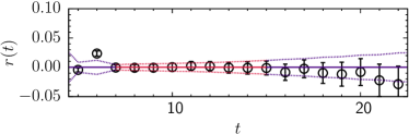
(a)  Residual

(b)  Effective Mass

Figure 1: Correlated fit results for a pseudoscalar heavy-light meson correlator generated with the OK action at $\kappa=0.041$ and $\bm{p}=\bm{0}$. In Fig. 1(a), the outer dotted lines show the statistical error of the fit. In Fig. 1(b), the fit result for the ground-state energy $E$ is denoted by the horizontal red line plotted over the chosen fit interval.

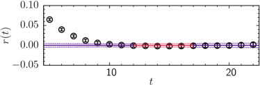
(a)  Residual

(b)  Effective Mass

Figure 2: Correlated fit results for a pseudoscalar bottomonium correlator generated with the OK action at $\kappa=0.041$ and $\bm{p}=\bm{0}$. In Fig. 2(a), the outer dotted lines show the statistical error of the fit. In Fig. 2(b), the fit result for the ground-state energy $E$ is denoted by the horizontal red line plotted over the chosen fit interval.

Table 3: Dispersion fit results for heavy-light mesons with masses near those of the $D_{s}^{(\ast)}$ and $B_{s}^{(*)}$. The energies $E$ are from the correlator fits to the function in Eq. (30). The first column indicates the lattice action and the (approximate) heavy-quark flavor. The second column is the hopping parameter $\kappa$. The following columns are the rest mass $M_{1}$, the kinetic mass $M_{2}$, the generalized masses $M_{4}$ and $M_{6}$, and the coefficient of an $O(3)$ symmetry breaking term $W_{4}$. The last two columns are the $\chi^{2}$ divided by the degrees of freedom (dof) $N_{\text{data}}-N_{\text{param}}$, $p$-value. All ten momenta data points are included in the dispersion relation fit; these spectra are obtained from the correlator fits to Eq. (25) which include all correlations. Fits to the dispersion relation include all correlations among different momenta. Errors are all from a single-elimination jackknife.

Action ($Q$)	$\kappa$	$M_{1}$	$M_{2}$	$M_{4}$	$W_{4}\times 10^{2}$	$M_{6}$	$\chi^{2}/\text{dof}$	$p$
OK ($b$-like)	$0.039$	$2.2141(24)$	$3.924(63)$	$2.50(16)$	$-6.1(7)$	–	$1.13(4)$	$0.34(2)$
	$0.040$	$2.1261(22)$	$3.580(53)$	$2.46(15)$	$-5.5(8)$	–	$1.21(4)$	$0.30(2)$
	$0.041$	$2.0345(19)$	$3.256(45)$	$2.40(15)$	$-4.9(9)$	–	$1.26(4)$	$0.27(2)$
	$0.042$	$1.9382(17)$	$2.952(37)$	$2.33(15)$	$-4.0(1.0)$	–	$1.35(4)$	$0.23(2)$
OK ($c$-like)	$0.0468$	$1.3742(9)$	$1.663(12)$	$1.59(7)$	$3.0(2.4)$	–	$1.29(4)$	$0.26(2)$
	$0.048$	$1.1861(8)$	$1.362(8)$	$1.33(4)$	$6.8(3.5)$	$1.4(2)$	$1.47(5)$	$0.20(2)$
	$0.049$	$1.0003(7)$	$1.104(6)$	$1.12(3)$	$7.3(5.5)$	$1.2(1)$	$1.47(5)$	$0.20(2)$
	$0.050$	$0.7688(5)$	$0.827(5)$	$0.85(2)$	$7.4(10.2)$	$1.0(1)$	$0.32(2)$	$0.90(1)$
FL ($b$-like)	$0.083$	$2.0668(31)$	$3.250(83)$	$2.47(46)$	$2.4(1.3)$	–	$0.50(3)$	$0.81(2)$
	$0.091$	$1.8835(28)$	$2.746(70)$	$2.28(43)$	$3.3(1.8)$	–	$0.48(3)$	$0.83(2)$
FL ($c$-like)	$0.121$	$1.1533(8)$	$1.308(9)$	$1.20(4)$	$12.9(4.5)$	$1.4(2)$	$1.38(5)$	$0.23(2)$
	$0.127$	$0.9736(6)$	$1.048(9)$	$0.97(5)$	$16.9(7.2)$	$1.1(1)$	$0.83(4)$	$0.53(3)$

(a)  Pseudoscalar

Action ($Q$)	$\kappa$	$M_{1}$	$M_{2}$	$M_{4}$	$W_{4}\times 10^{2}$	$M_{6}$	$\chi^{2}/\text{dof}$	$p$
OK ($b$-like)	$0.039$	$2.2330(31)$	$3.988(87)$	$2.69(30)$	$-4.5(1.0)$	–	$1.36(4)$	$0.23(2)$
	$0.040$	$2.1475(28)$	$3.653(74)$	$2.60(28)$	$-4.1(1.1)$	–	$1.23(4)$	$0.29(2)$
	$0.041$	$2.0589(25)$	$3.325(61)$	$2.53(27)$	$-3.7(1.2)$	–	$1.20(4)$	$0.31(2)$
	$0.042$	$1.9662(23)$	$3.016(50)$	$2.47(27)$	$-3.1(1.3)$	–	$1.18(4)$	$0.31(2)$
OK ($c$-like)	$0.0468$	$1.4324(14)$	$1.733(18)$	$1.74(14)$	$2.9(3.6)$	–	$1.04(4)$	$0.39(2)$
	$0.048$	$1.2594(13)$	$1.443(15)$	$1.48(10)$	$4.5(5.7)$	–	$0.97(4)$	$0.45(2)$
	$0.049$	$1.0921(12)$	$1.205(13)$	$1.27(9)$	$4.2(9.6)$	–	$0.78(3)$	$0.59(3)$
	$0.050$	$0.8920(14)$	$0.969(15)$	$0.98(7)$	$-8.8(21.7)$	–	$0.35(2)$	$0.91(1)$
FL ($b$-like)	$0.083$	$2.0906(53)$	$3.406(132)$	$3.18(2.29)$	$0.6(1.9)$	–	$0.27(2)$	$0.95(1)$
	$0.091$	$1.9157(37)$	$2.890(74)$	$2.68(91)$	$1.0(2.9)$	–	$0.54(3)$	$0.78(2)$
FL ($c$-like)	$0.121$	$1.2287(15)$	$1.438(19)$	$1.43(10)$	$10.7(5.5)$	–	$0.58(3)$	$0.75(2)$
	$0.127$	$1.0693(16)$	$1.206(17)$	$1.24(8)$	$12.7(9.2)$	–	$0.67(3)$	$0.67(2)$

(b)  Vector

Table 4: Dispersion fit results for quarkonium. The energies $E$ are from the correlator fits to the function in Eq. (30). The first column indicates the lattice action and the (approximate) heavy-quark flavor. The second column is the hopping parameter $\kappa$. The following columns are the rest mass $M_{1}$, the kinetic mass $M_{2}$, the generalized masses $M_{4}$ and $M_{6}$, and the coefficient of an $O(3)$ symmetry breaking terms $W_{4}$ and $W_{6}^{\prime}$. The last two columns are the $\chi^{2}$ divided by the degrees of freedom (dof) $N_{\text{data}}-N_{\text{param}}$, $p$-value. All ten momenta data points are included in the dispersion relation fit; these spectra are obtained from the correlator fits to Eq. (25), setting $R_{i}^{p}=0$, which include all correlations; $R_{1}=0$ for bottomonium fits. Fits to the dispersion relation include all correlations among different momenta. Errors are all from a single-elimination jackknife.

Action ($Q$)	$\kappa$	$M_{1}$	$M_{2}$	$M_{4}$	$W_{4}\times 10^{2}$	$M_{6}$	$W_{6}^{\prime}\times 10^{4}$	$\chi^{2}/\text{dof}$	$p$
OK ($b$-like)	$0.039$	$3.5200(4)$	$6.637(19)$	$4.58(8)$	$-0.91(3)$	–	–	$0.51(3)$	$0.80(2)$
	$0.040$	$3.3616(4)$	$6.120(17)$	$4.38(8)$	$-0.97(3)$	–	–	$0.48(3)$	$0.82(2)$
	$0.041$	$3.1968(4)$	$5.601(16)$	$4.16(8)$	$-0.99(4)$	–	–	$0.95(4)$	$0.46(3)$
	$0.042$	$3.0242(4)$	$5.083(14)$	$3.90(7)$	$-0.97(5)$	–	–	$1.32(4)$	$0.25(2)$
OK ($c$-like)	$0.0468$	$2.0169(5)$	$2.647(11)$	$2.41(9)$	$0.7(4)$	–	–	$0.59(3)$	$0.74(2)$
	$0.048$	$1.6819(5)$	$2.063(8)$	$1.97(6)$	$2.1(7)$	–	–	$0.82(3)$	$0.55(3)$
	$0.049$	$1.3516(5)$	$1.574(5)$	$1.54(3)$	$3.6(1.5)$	–	–	$1.20(4)$	$0.30(2)$
	$0.050$	$0.9419(5)$	$1.056(4)$	$1.08(2)$	$-0.6(4.1)$	–	–	$1.36(4)$	$0.23(2)$
FL ($b$-like)	$0.083$	$3.1765(3)$	$9.392(23)$	$3.69(2)$	$1.84(2)$	$4.1(1)$	$5.6(3)$	$0.77(3)$	$0.55(2)$
	$0.091$	$2.8764(3)$	$6.894(18)$	$3.19(2)$	$2.45(4)$	$4.0(3)$	$9.2(6)$	$0.75(4)$	$0.56(3)$
FL ($c$-like)	$0.121$	$1.6216(5)$	$2.128(9)$	$1.69(3)$	$8.5(7)$	$1.8(1)$	–	$1.39(5)$	$0.23(2)$
	$0.127$	$1.3087(5)$	$1.561(6)$	$1.35(2)$	$12.0(1.5)$	$1.4(1)$	–	$0.83(4)$	$0.53(3)$

(a)  Pseudoscalar

Action ($Q$)	$\kappa$	$M_{1}$	$M_{2}$	$M_{4}$	$W_{4}\times 10^{2}$	$M_{6}$	$W_{6}^{\prime}\times 10^{4}$	$\chi^{2}/\text{dof}$	$p$
OK ($b$-like)	$0.039$	$3.5393(4)$	$6.626(20)$	$4.69(9)$	$-0.99(3)$	–	–	$0.64(3)$	$0.70(2)$
	$0.040$	$3.3827(4)$	$6.116(19)$	$4.48(10)$	$-1.04(4)$	–	–	$0.69(3)$	$0.66(2)$
	$0.041$	$3.2201(4)$	$5.606(17)$	$4.25(10)$	$-1.05(5)$	–	–	$1.03(4)$	$0.40(2)$
	$0.042$	$3.0500(4)$	$5.096(16)$	$3.98(9)$	$-1.00(6)$	–	–	$1.36(4)$	$0.23(2)$
OK ($c$-like)	$0.0468$	$2.0657(7)$	$2.686(14)$	$2.55(12)$	$1.1(5)$	–	–	$0.43(2)$	$0.86(2)$
	$0.048$	$1.7425(7)$	$2.112(10)$	$2.08(9)$	$2.8(9)$	–	–	$0.49(3)$	$0.81(2)$
	$0.049$	$1.4280(7)$	$1.640(8)$	$1.63(5)$	$4.5(1.7)$	–	–	$0.66(3)$	$0.68(2)$
	$0.050$	$1.0497(9)$	$1.154(7)$	$1.15(3)$	$-1.7(5.9)$	–	–	$0.76(3)$	$0.60(3)$
FL ($b$-like)	$0.083$	$3.1939(3)$	$9.589(25)$	$3.70(2)$	$1.82(2)$	$4.0(1)$	$5.4(3)$	$1.53(6)$	$0.19(2)$
	$0.091$	$2.8987(4)$	$7.035(20)$	$3.21(2)$	$2.43(4)$	$4.0(3)$	$9.0(5)$	$0.44(3)$	$0.78(2)$
FL ($c$-like)	$0.121$	$1.6774(8)$	$2.235(13)$	$1.75(5)$	$7.6(9)$	$1.9(2)$	–	$1.05(4)$	$0.39(2)$
	$0.127$	$1.3808(9)$	$1.680(11)$	$1.43(4)$	$10.0(2.0)$	$1.6(1)$	–	$0.50(3)$	$0.78(2)$

(b)  Vector

We carry out correlated fits with a statistical estimate of the covariance matrix $\mathrm{cov}(t,t^{\prime})$ between different time slices $t$ and $t^{\prime}$,

$$\mathrm{cov}(t,t^{\prime})=\frac{1}{\mathcal{N}}\sum_{i=1}^{N_{\text{cfg}}}\left[C_{i}(t)-C(t)\right]\left[C_{i}(t^{\prime})-C(t^{\prime})\right],$$ (26)

where the normalization factor $\mathcal{N}=N_{\text{cfg}}(N_{\text{cfg}}-1)$, $C_{i}(t)$ represents the average over the $N_{\text{src}}$ sources for the $i^{\text{th}}$ gauge field, and the two-point correlator $C(t)=C^{M}(t,\bm{p})$ for a given meson type $M$ and momentum $\bm{p}$ is estimated with the ensemble average

$$C(t)=\frac{1}{N_{\text{cfg}}}\sum_{i=1}^{N_{\text{cfg}}}C_{i}(t).$$ (27)

To increase statistics, we take advantage of the structure of Eq. (24) and average the data for time separations $t$ and $T-t$. Then, we take the fit interval $[t_{\text{min}},t_{\text{max}}]$, where $0<t_{\text{min}}<t_{\text{max}}<T/2$, equal to $[7,15]$ for the heavy-light meson with the OK action and $[9,15]$ with the Fermilab action. For charmonium, the fit interval is $[9,14]$ for both actions. For bottomonium, the fit interval is $[12,17]$ for the OK action and $[14,19]$ for the Fermilab action. We fix these intervals for fits to all correlators, independent of hopping parameter $\kappa$, momentum $\bm{p}$, and pseudoscalar vs. vector channel.

The $t_{\text{min}}$ are chosen by observing the effective mass $m_{\text{eff}}(t)$ calculated from the definition

$$m_{\text{eff}}(t)=\frac{1}{2}\ln\left(\frac{C^{M}(t)}{C^{M}(t+2)}\right)$$ (28)

as well as comparing the fit results $E$ with the $m_{\text{eff}}(t)$. Figure 2 shows the effective mass $m_{\text{eff}}(t)$ and correlator fit residual $r(t)$

$$r(t)=\frac{C^{M}(t)-f(t)}{\lvert C^{M}(t)\rvert}$$ (29)

for a pseudoscalar heavy-light meson correlator generated with the OK action, $\kappa_{\text{OK}}=0.041$, and $\bm{p}=\bm{0}$. The pseudoscalar bottomonium correlator fit results obtained with the same action and parameters are given in Fig. 2. To estimate the statistical errors, we use a single-elimination jackknife.

IV Meson Masses

The dispersion relation of the mesons has the same form as that of the quarks with the quark masses $m_{1}$ and $m_{2}$ given in Eqs. (17) and (18), respectively, replaced by meson masses $M_{1}$ and $M_{2}$. The mismatch between the meson rest and kinetic masses can be exploited to test the improvement of nonrelativistically interpreted actions.

We fit the ground-state energy $E(\bm{p})$ in Eq. (25) for each momentum $\bm{p}$ to the nonrelativistic dispersion relation to obtain the rest mass $M_{1}$ and kinetic mass $M_{2}$ of each meson. Including terms up to $\mathrm{O}\!\left(\bm{p}^{6}\right)$, the dispersion relation is

$$E(\bm{p}) =M_{1}+\frac{\bm{p}^{2}}{2M_{2}}-\frac{(\bm{p}^{2})^{2}}{8M_{4}^{3}}+E_{4}^{\prime}+E_{6}+E_{6}^{\prime},$$ (30)

$$E_{4}^{\prime} =-\frac{a^{3}W_{4}}{6}\sum_{i}p_{i}^{4},$$ (31)

$$E_{6} =\frac{(\bm{p}^{2})^{3}}{16M_{6}^{5}},$$ (32)

$$E_{6}^{\prime} =\frac{a^{5}W_{6}^{\prime}}{2}\bm{p}^{2}\sum_{i}p_{i}^{4}-\frac{a^{5}W_{6}}{3}\sum_{i}p_{i}^{6}.$$ (33)

The $M_{4,6}$ are generalized masses; the rest mass $M_{1}$ and these generalized masses $M_{4,6}$ are expected El-Khadra et al. (1997); Oktay and Kronfeld (2008) to approach the kinetic mass $M_{2}$ in the continuum limit. The $O(3)$ rotation-symmetry-breaking terms are $E_{4}^{\prime}$ and $E_{6}^{\prime}$. In the continuum limit, the coefficients $a^{3}W_{4}$, $a^{5}W^{\prime}_{6}$, and $a^{5}W_{6}$ vanish. We fit the simulation data for $E(\bm{p})$ to the the right-hand side of Eq. (30), taking the full covariance matrix among the different momentum channels, and investigate variations by excluding some or all of the higher-order terms $E_{4}^{\prime}$, $E_{6}$, and $E_{6}^{\prime}$. We do not introduce priors here. The seven fit parameters are $M_{1}$, $M_{2}^{-1}$, $M_{4}^{-3}$, $M_{6}^{-5}$, $W_{4}$, $W^{\prime}_{6}$, and $W_{6}$. We find that we do not need all seven terms in the dispersion relation. In many cases, it suffices to keep only the first five, while some fits give better $p$ values with the first six.

For the pseudoscalar heavy-light meson, as the spectrum becomes more relativistic, $M_{2}$ approaches $M_{1}$, and including the $E_{6}$ term results in a better fit. Because the vector heavy-light meson spectrum has a larger statistical error than the pseudoscalar meson spectrum, the $E_{6}$ term is not only determined to be statistically zero, but also does not improve the fit. The $E_{6}$ term also improves the fit for the charmonium spectrum with the Fermilab action.

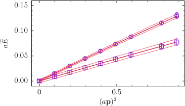
(a)  OK

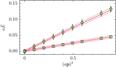
(b)  Fermilab

Figure 3: The pseudoscalar heavy-light meson (circle) and quarkonium (square) subtracted energies $\widetilde{E}$ [Eq. (34)] as a function of $(a\bm{p})^{2}$ for (a) the OK action at $\kappa=0.041$ and (b) the Fermilab (clover) action at $\kappa=0.083$. The lines show fits to Eq. (30). The errors are from a single-elimination jackknife. In these plots, the errors for the bottomonium data points and fit lines are scaled by a factor 10. The behavior for vector mesons is similar, apart from the larger statistical errors.

The $W_{6}^{\prime}$ term in addition to the $E_{6}$ term improves the fit for the bottomonium spectrum with the Fermilab action. Note that the correlator fit for bottomonium does not include any excited states., although including a single excited state is statistically consistent, when fitting Eq. (30) without the $E_{6}$ and $E_{6}^{\prime}$ terms. We use the fits with excited states to cross-check the single-state fits. We observed the same behavior with the two-state fit for the bottomonium spectrum with the OK action. Note that the bottomonium spectrum for the OK action still results in a good fit without the $E_{6}$ and $E_{6}^{\prime}$ terms, when the correlator fit only accounts for the ground state.

Figure 3 shows the dispersion relation fits to the pseudoscalar heavy-light meson and quarkonium data generated with the OK (Fermilab) action with $\kappa_{\text{OK}}=0.041$ ($\kappa_{\text{FL}}=0.083$). We plot the dispersion relation fit results after subtracting the rest mass and the higher-order term $E_{4}^{\prime}$. We thus define

$$\widetilde{E}=E-M_{1}-E_{4}^{\prime}$$ (34)

to draw the plot. As one can see from Fig. 3, the slope—and, hence, the kinetic mass $M_{2}$—is reliably determined from fits to Eq. (30). Interestingly, the OK action leads to statistical errors noticeably smaller than those from the Fermilab action, especially for the heavy-light masses.

The fit results for the heavy-light mesons are summarized in Tables 4(a) and 4(b). They are obtained from correlated fits. From these tables for the heavy-light mesons, one can see that the higher-order generalized mass $M_{4}$ approaches the kinetic mass $M_{2}$ as the kinetic mass decreases. The rest mass $M_{1}$ also approaches the kinetic mass $M_{2}$. Note that $M_{4}$ does not necessarily agree better with $M_{2}$ for the OK action, even though the OK action tunes the action such that $m_{4}=m_{2}$. A possible explanation is that the binding energy $M_{4}-m_{4}$ stems from higher-dimension effects not yet incorporated into the OK action.

The correlated fit results for quarkonia are summarized in Tables 5(a) and 5(b). For the charmonium results obtained with the OK action, $M_{4}$ is closer to the kinetic mass $M_{2}$ than to the rest mass $M_{1}$, but for the Fermilab action $M_{4}$ is closer to $M_{1}$. In the bottomonium region, $M_{4}$ is closer to the rest mass $M_{1}$ than the kinetic mass $M_{2}$ for both actions. The difference $M_{2}-M_{1}$ is large for the Fermilab action at $\kappa_{\text{FL}}=0.083$, $0.091$, but it is diminished with the OK action at the comparable values $\kappa_{\text{OK}}=0.039$, $0.040$, $0.041$, $0.042$. However, even with the OK action, the difference between $M_{4}$ and $M_{2}$ in the bottomonium spectra is larger than that in the heavy-light meson spectra.

V The “Inconsistency” Collins et al. (1996)

To study how the Fermilab method works, Ref. Collins et al. (1996) introduced the quantity

$$I=\frac{2{\delta}M_{\overline{Q}q}-({\delta}M_{\overline{Q}Q}+{\delta}M_{\overline{q}q})}{2M_{2\overline{Q}q}},$$ (35)

where

$$\delta M_{\overline{Q}q}=M_{2\overline{Q}q}-M_{1\overline{Q}q}.$$ (36)

The combination $I$ should vanish, even when the quark rest masses $m_{1}$ are mistuned. If $I$ does not vanish, it means that the action contains nontrivial discretization effects at higher order in the HQET or NRQCD power counting, so $I$ is often called the “inconsistency.” In fact, as we reproduce below, $I\neq 0$ for the Fermilab action Collins et al. (1996) (unless $m_{2}a\ll 1$), as one can see in Eq. (40).

The explanation is as follows Kronfeld (1997). The meson masses $M_{i}$ $(i=1,2)$ can be written as a sum of the quark masses $m_{i}$ and the binding energy:

$$M_{i\overline{Q}q}=m_{i\overline{Q}}+m_{iq}+B_{i\overline{Q}q},$$ (37)

which defines $B_{i}$. Upon substituting Eq. (37) into Eqs. (36) and (35), the quark masses cancel out, and the inconsistency becomes a relation among the binding energies,

$$I=\frac{2{\delta}B_{\overline{Q}q}-({\delta}B_{\overline{Q}Q}+{\delta}B_{\overline{q}q})}{2M_{2\overline{Q}q}},$$ (38)

where

$$\delta B_{\overline{Q}q}=B_{2\overline{Q}q}-B_{1\overline{Q}q}.$$ (39)

The quantities in Eqs. (36), (37), and (39) for heavy ($\overline{Q}Q$) and light ($\overline{q}q$) quarkonium are defined similarly. Because light quarks always have $ma\ll 1$, the $\mathrm{O}((ma)^{2})$ distinction between rest and kinetic masses is negligible for them, so we omit $\delta M_{\bar{q}q}$ (or $\delta B_{\bar{q}q}$) when computing $I$. The rest-mass binding energy $B_{1}$ is sensitive to effects of $\mathrm{O}(\lambda)$ or $\mathrm{O}(v^{2})$, while the kinetic-mass binding energy $B_{2}$ is sensitive to effects of $\mathrm{O}(\lambda^{3})$ or $\mathrm{O}(v^{4})$, with their larger relative discretization errors (for the clover and Fermilab actions). The discretization errors can be studied in the nonrelativistic limit via the Breit equation, yielding Kronfeld (1997); Bernard et al. (2011)

$$\delta B_{\overline{Q}q} =\frac{5}{3}\frac{\langle\bm{p}^{2}\rangle}{2\mu_{2}}\left[\mu_{2}\left(\frac{m_{2\overline{Q}}^{2}}{m_{4\overline{Q}}^{3}}+\frac{m_{2q}^{2}}{m_{4q}^{3}}\right)-1\right]$$ (40)

$$\hskip 12.0pt+\frac{4}{3}a^{3}\frac{\langle\bm{p}^{2}\rangle}{2\mu_{2}}\mu_{2}\left[w_{4\overline{Q}}m_{2\overline{Q}}^{2}+w_{4q}m_{2q}^{2}\right]+\mathrm{O}(\bm{p}^{4})$$

in the $S$ wave, where the reduced mass $\mu_{2}^{-1}=m_{2\overline{Q}}^{-1}+m_{2q}^{-1}$, and $m_{2}$, $m_{4}$, and $w_{4}$ are defined through the quark analog of Eq. (30). Here, $\bm{p}$ is the relative momentum of $\overline{Q}$ and $q$ in their center of mass. The OK action matches $m_{4}=m_{2}$ and $w_{4}=0$ at the tree level, so the two expressions in square brackets are of order $\alpha_{s}$. Because we use a tadpole-improved action, these one-loop errors are expected to be small.

(a)  Spin average

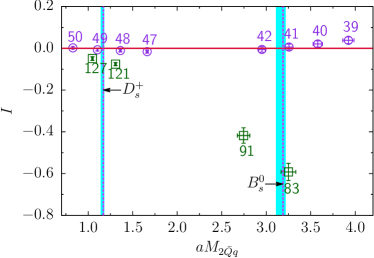
(b)  Pseudoscalar

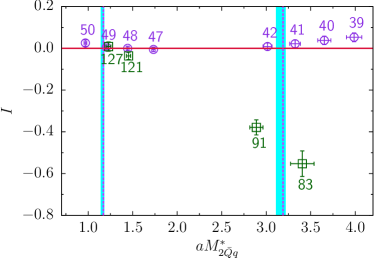
(c)  Vector

Figure 4: Inconsistency $I$ for (a) the spin averaged mass $\overline{M}=\frac{1}{4}(M+3M^{*})$, (b) pseudoscalar-meson mass, and (c) vector-meson mass. Data labels denote the value of $\kappa\times 10^{3}$. The purple circles (green squares) represents the OK (Fermilab) action. The errors are from the jackknife. Vertical lines with bands represent the physical masses from the PDG Patrignani et al. (2016) with experimental and (asymmetric) lattice-spacing errors added in quadrature. For the OK action $I$ almost vanishes (cf. horizontal red line), but for the Fermilab action it does not.

We calculate the inconsistency $I$ from the pseudoscalar and vector masses presented in Sec. IV. The derivation of Eq. (40) does not include spin-dependent effects, which should contribute to $I$ for both pseudoscalar and vector channels. To separate spin-dependent effects, which are the subject of Sec. VI, from spin-independent ones, we form the spin-averaged mass,

$$\overline{M}=\frac{1}{4}(M+3M^{*}),$$ (41)

writing $M$ ($M^{*}$) for pseudoscalar (vector) masses. We calculate the quantity $I$ with such spin-averaged rest and kinetic masses and plot the result in Fig. 4(a). For orientation, we also show the physical $B_{s}$ and $D_{s}$ masses (for this ensemble) with vertical bands. We find that $I$ is close to 0 for the OK action even in the $b$-like region, whereas the Fermilab action leads to a very large deviation $I\approx-0.6$ from the continuum value, $I=0$, as in Ref. Collins et al. (1996). This outcome provides good numerical evidence that the improvement of spin-independent effects of the OK action is realized in practice. The small $I$ remaining stems from still higher-dimension kinetic operators of $\mathrm{O}(\lambda^{4})$ in HQET, or $\mathrm{O}(v^{7})$ in NRQCD, power counting, which are not addressed by the OK action. For completeness, Figs. 4(b) and (c) show $I$ for the pseudoscalar and vector channels, demonstrating that spin-dependent effects do not alter the conclusions.

VI Hyperfine Splittings

The hyperfine splitting is the difference in the masses of the vector and pseudoscalar mesons:

$$\Delta_{1} =M_{1}^{\ast}-M_{1},$$ (42)

$$\Delta_{2} =M_{2}^{\ast}-M_{2}.$$ (43)

From Eq. (39), one has

$$\Delta_{2}-\Delta_{1}=\delta{B^{\ast}}-\delta{B}.$$ (44)

Spin-independent contributions cancel in this binding-energy difference, so the hyperfine difference $\Delta_{2}-\Delta_{1}$ diagnoses the improvement of the spin-dependent $c_{3}$ and $c_{5}$ terms of $\mathrm{O}(\lambda^{3})$ in HQET power counting, or $\mathrm{O}(v^{6})$ in NRQCD.

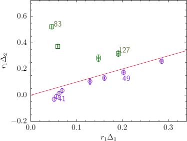
(a)  Quarkonium

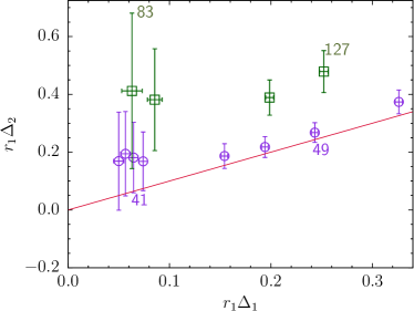
(b)  Heavy-light meson

Figure 5: Hyperfine splitting $\Delta_{2}$ obtained from the kinetic masses vs. $\Delta_{1}$, obtained from the rest masses. The square (green) represents the Fermilab action data, and the circle (purple) represents the OK action data. The labels are $\kappa\times 10^{3}$, corresponding to kinetic masses close to the physical $B_{s}$ (83, 41) and $D_{s}$ (49, 127) masses, as shown in Fig. 4. The continuum limit is represented by the line (red) $\Delta_{2}=\Delta_{1}$. Errors are from the jackknife.

As one can see in Fig. 5(a), the OK action shows clear improvement for quarkonium. The data points from the OK action lie much closer to the continuum value $\Delta_{2}=\Delta_{1}$ (the red line) for all simulated values of $\kappa_{\text{OK}}$; in the charmonium region, they remain consistent with the continuum line within the error. The heavy-light results in Fig. 5(b) also show clear improvement in the region near the $D_{s}$ mass. The results with the OK action remain consistent with the continuum limit throughout the $B_{s}$ mass region, but the improvement is not yet statistically significant. Higher statistics would resolve the issue. All in all, the hyperfine splittings show the improvement from the higher-dimension chromomagnetic interactions—those with couplings $c_{3}$ and $c_{5}$.

For both quarkonia and heavy-light mesons, the hyperfine splitting of the kinetic mass, $\Delta_{2}$, has a larger error than that of the rest mass, $\Delta_{1}$, because the kinetic mass requires correlators with $\bm{p}\neq\bm{0}$, which are noisier than those with $\bm{p}=\bm{0}$. As the rest mass $M_{1}$ and the kinetic mass $M_{2}$ are determined with smaller error with the OK action than the Fermilab action (see Sec. IV), the statistical errors shown for the hyperfine splittings $\Delta_{1}$ and $\Delta_{2}$ in Fig. 5 are smaller with the OK action, especially in the case of $\Delta_{2}$.

VII Conclusions

Our tests of the Fermilab improvement program are based on the two-point correlators for mesons generated with the Fermilab El-Khadra et al. (1997) and OK Oktay and Kronfeld (2008) actions. Looking ahead to phenomenological applications Bailey et al. (2015b, 2016b); Jeong et al. (2016), we have chosen four hopping parameters for the OK action in each of the $b$- and $c$-quark mass regions. For the Fermilab action, we have simulated two $b$-like and two $c$-like hopping parameters. Although the lattice data span the physically interesting regions, the central aim of this paper is to test the improvement theory of Refs. El-Khadra et al. (1997); Oktay and Kronfeld (2008) against simulation data, independent of the phenomenological interpretation of the action’s parameters.

We focus on tests of both the spin-independent and spin-dependent terms in the OK action. The results for the (spin-averaged) quantity $I$, known as the inconsistency Collins et al. (1996), show that the OK action succeeds in improving the effects that generate the kinetic-mass binding energy. The hyperfine splitting shows that the OK action significantly improves the higher-dimension spin-dependent, chromomagnetic effects, at least in quarkonium. For the heavy-light system, the data show a clear improvement for smaller $c$-like masses, but in the $b$-like region, large statistical errors prevent us from reaching firm conclusions.

This study has yielded some noteworthy byproducts. As $am_{0}$ is reduced, here with fixed $a\approx 0.12$ fm, the meson masses $M_{1}$, $M_{2}$, and $M_{4}$ approach each other, verifying the expectations of the Fermilab and OK actions. The difference between $M_{4}$ and $M_{2}$, for $am_{2}\not\ll 1$, is not much better for the OK action than the Fermilab action. By analogy with the inconsistency $I$ Collins et al. (1996); Kronfeld (1997), this feature is probably explained by the associated binding energy $M_{4}-m_{4}$, which stems from higher-dimension effects not improved by the OK action. Finally, in the $b$-like region, $am_{2}\sim 3$, the OK action produces statistically more precise results than the Fermilab action for the heavy-light correlator energies and, hence, the masses $M_{2}$ and $M_{4}$.

As an application of the OK action, a calculation of the form factors for the $B\to D^{(*)}\ell\nu$ semileptonic decays is underway, with the aim of determining the CKM matrix element $|V_{cb}|$. To achieve the desired sub-percent precision on the relevant form factors, it will be necessary to derive the analog of the OK action for currents Bailey et al. (2016b, 2015b), and to calculate the renormalization. Meanwhile some of us are extending the present work to a full-fledged tuning run Jeong et al. (2016).