Assessing Uncertainties in X-ray Single-particle Three-dimensional reconstructions

Abstract.

Modern technology for producing extremely bright and coherent X-ray laser pulses provides the possibility to acquire a large number of diffraction patterns from individual biological nanoparticles, including proteins, viruses, and DNA. These two-dimensional diffraction patterns can be practically reconstructed and retrieved down to a resolution of a few Ångström. In principle, a sufficiently large collection of diffraction patterns will contain the required information for a full three-dimensional reconstruction of the biomolecule. The computational methodology for this reconstruction task is still under development and highly resolved reconstructions have not yet been produced.

We analyze the Expansion-Maximization-Compression scheme, the current state of the art approach for this very challenging application, by isolating different sources of uncertainty. Through numerical experiments on synthetic data we evaluate their respective impact. We reach conclusions of relevance for handling actual experimental data, as well as pointing out certain improvements to the underlying estimation algorithm.

We also introduce a practically applicable computational methodology in the form of bootstrap procedures for assessing reconstruction uncertainty in the real data case. We evaluate the sharpness of this approach and argue that this type of procedure will be critical in the near future when handling the increasing amount of data.

1. Introduction

Determing the structure of a very small biological object, such as a protein or a virus, is both fascinating and hard. The most classical and common way to determine the atomic and molecular structures of small biological objects is to crystallize them and use X-rays to investigate the resulting macroscopic crystals. This method, X-ray crystallography, has succeeded in determining more than 97,200 structures [24]. With X-ray crystallography, high-quality structures can be obtained from crystals whose atoms are formed in a near perfect periodic arrangement. However, due to conformational flexibility not all biological samples can form crystals.

Modern X-ray Free Electron Laser (X-FEL) technology potentially provides the ability to determine biological structure without crystals. X-FEL pulses are intense and short enough to create an observable diffraction signal from one single particle, outrunning the radiation damage. Digital detectors are used to capture the diffracted wave, depicting the sample before it explodes and turns into a plasma. This approach is called “diffract and destroy” [23], and has caught considerable attention in structural biology [14, 5, 3, 22, 16, 11].

For a Flash X-ray single particle diffraction Imaging (FXI) experiment, a stream of particles are injected into the X-ray beam, and hit by the extremely intense X-ray pulses, producing diffraction patterns showing the illuminated objects. The energy from the X-ray pulse destroys the sample, so it is impossible to collect successive exposures of the same particle. However, since many biological particles exist in identical copies at the resolution scales of relevance, the diffraction patterns can be treated approximately as differently oriented exposures of the same particle. The particle rotations can be recovered [20, 6, 2] by maximizing the fit among all diffraction patterns. Hence, a 3D intensity can be assembled as an average of these oriented patterns.

In 2011, a 2D reconstruction of a mimivirus [25] was reported, one of the largest known viruses at a diameter of roughly 500 nm. The reconstruction was based on individual FXI diffraction patterns, with 32-nm full-period resolution. Later, a corresponding 3D reconstruction was also presented [11], whose resolution was markedly inferior to the one achieved in 2D from individual patterns. The authors of the 3D reconstruction suggested that a higher-resolution 3D reconstruction could be obtained by adding more diffraction patterns from homogeneous samples. This would clearly require a large and high quality dataset along with a comprehensive understanding of the uncertainty propagation in the reconstruction procedure.

In this paper, we attempt to analyze sources and propagation of uncertainties in the Expansion-Maximization-Compression (EMC) algorithm [20, 21], the best-in-practice 3D reconstruction method, in order to be able to estimate the 3D reconstruction resolution.

An overview of the computational methodology using FXI images is found in §2. We discuss the sources of errors and introduce two bootstrap schemes for estimating the reconstruction uncertainty in §3. Numerical experiments to assess the impact of the various sources of uncertainty are presented in §4, where we also evaluate the sharpness of the bootstrap estimators and the robustness of the overall reconstruction procedure. A concluding discussion is found in §5.

2. Imaging via FXI

It is well known that one can use the Fourier transform to approximate diffracted waves in the far-field [13]. In this section, we review the relationship between the solutions to the wave equation as represented via Fourier transforms and the captured FXI diffraction images. We also review Maximum Likelihood-based image processing techniques, and the best-in-practice 3D FXI reconstruction algorithm.

2.1. Scattering theory

X-FEL pulses can produce diffraction patterns of single biomolecules. This diffraction process, a wave propagation in free space, is described by the Helmholtz wave equation,

(2.1) $$\nabla^{2}\Psi+\mathit{k}^{2}\mathit{n}^{2}\Psi =0,$$

where the wave number is $\mathit{k}$, and the refractive index is $\mathit{n}$.

We can solve the wave equation on an Ewald sphere, which is perpendicular to the X-ray beam direction, by assuming that: i) the polarization of X-FEL pulses can be ignored; ii) the objects in the X-ray beam are small, so that photons diffract only once inside the object (i.e. only the first order Born approximation $\Psi_{1}$ is required); iii) small-angle scattering is assumed, i.e. that the object-detector distance is much longer than the wavelength; iv) the X-FEL sources generate plane, coherent, and homogeneous waves.

The scattered wave on the Ewald sphere can then be written as follows:

(2.2) $$\bar{\Psi}\approx\sqrt{I_{0}\Omega_{p}}\frac{2\pi}{\lambda^{2}}\mathscr{F}_{2}\{\delta\mathit{n}_{\perp}(\mathbf{r}_{\perp})\}\Delta x^{3}\propto\mathscr{F}_{2}\{\delta\mathit{n}_{\perp}(\mathbf{r}_{\perp})\},$$

where $\mathscr{F}_{2}$ is a 2D Fourier transformation, $\Delta x$ is the sampling distance, $\delta\mathit{n}_{\perp}(\mathbf{r}_{\perp})$ is the refractive component of the refractive index for the Ewald sphere, $I_{0}$ is the X-ray pulse intensity at the object-beam interaction point, and $\lambda$ is the wave length. Further, $\Omega_{p}$ equals to $P^{2}/D^{2}$, where $P$ is the physical pitch of a single detector pixel, and $D$ is the object-detector distance.

The noiseless diffraction pattern detected by the detector is the square of this scattered wave, i.e.

(2.3) $$I=|\bar{\Psi}|^{2}\propto|\mathscr{F}_{2}\{\delta\mathit{n}_{\perp}(\mathbf{r}_{\perp})\}|^{2}.$$

We denote a collection of noiseless diffraction patterns by $K^{*}=(K^{*}_{k})_{k=1}^{M_{\mbox{{\tiny data}}}}$, where each frame $K^{*}_{k}$ is obtained from (2.3) by specifying effectively a rotation of the object. Since the X-ray pulse intensity at the object-beam interaction point $I_{0}$ will vary in practice, we denote this variation by $\phi$ - the (photon) fluence, such that diffraction pattern with varying fluence is obtained by scaling $\phi K^{*}_{k}$. Moreover, since digital detectors are pixelized, we also discretize each diffraction pattern and write $K^{*}_{k}=(K^{*}_{ik})_{i=1}^{M_{\mbox{{\tiny pix}}}}$, where $M_{\mbox{{\tiny pix}}}$ is the number of pixels.

2.2. Maximum-Likelihood-based Imaging for FXI

In (2.2), the refractive component of the refractive index for the Ewald sphere $\delta\mathit{n}_{\perp}(\mathbf{r}_{\perp})$ is dependent on the rotation of particle. This is directly observable from FXI experiments. Several methods [20, 2, 6] can be used to estimate the unknown particle rotations from FXI diffraction patterns, but the most successful approach so far is the EMC algorithm [11, 21, 20]. Besides calculating maximum-likelihood (ML) estimates, the EMC algorithm interpolates between 2D diffraction patterns and a 3D model.

The EMC algorithm consists of 4 steps per iteration: i) the expansion step (e step) slices the 3D model through the model center according to the sampled rotation, i.e. expands the 3D model into a set of 2D slices; ii) the expectation step (E step) estimates the probability of each pattern to be in any given rotation; iii) the maximization step (M step) updates the 2D slices and their fluences using the estimated rotational probability; iv) the compression step (C step) inserts the updated 2D slices back into the 3D model.

We first introduce the e and the C step, which interpolates between a 3D model and 2D slices. Let $\mathbb{W}=\{\mathbb{W}_{l}\}_{l=1}^{M_{\mbox{{\tiny grid}}}}$ be a 3D discrete model, an estimation of the 3D Fourier intensity of a biomolecule, where $M_{\mbox{{\tiny grid}}}=M_{\mbox{{\tiny pix}}}^{3/2}$. The rotational space $R$ is discretized by $(R_{j})_{j=1}^{M_{\mbox{{\tiny rot}}}}$, and the corresponding prior weight for rotation $R_{j}$ is $w_{j}$, normalized such that $\sum_{j}w_{j}=1$. Similarly, the intensity space is discretized by a set of pixels $(q_{i})_{i=1}^{M_{\mbox{{\tiny pix}}}}$, such that the unknown 2D Fourier intensity at position $R_{j}q_{i}$ can be denoted by $W_{ij}$ in this coordinate system. We define interpolation weights $f$ and interpolation abscissas $(p_{l})_{l=1}^{M_{\mbox{{\tiny grid}}}}$ such that for $g$ some smooth function,

(2.4) $$g(q)\approx\sum_{l=1}^{M_{\mbox{{\tiny grid}}}}f(p_{l}-q)g(p_{l}).$$

An e step slices $W_{j}$ from the 3D model $\mathbb{W}$ as follows:

(2.5) $$W_{ij} =\sum_{l=1}^{M_{\mbox{{\tiny grid}}}}f(p_{l}-R_{j}q_{i})\mathbb{W}_{l}.$$

The C step inverses the interpolation of the e step by inserting the 2D slices back into the 3D grid,

(2.6) $$\mathbb{W}_{l} =\frac{\sum_{i=1}^{M_{\mbox{{\tiny pix}}}}\sum_{j=1}^{M_{\mbox{{\tiny rot}}}}f(p_{l}-R_{j}q_{i})W_{ij}}{\sum_{i=1}^{M_{\mbox{{\tiny pix}}}}\sum_{j=1}^{M_{\mbox{{\tiny rot}}}}f(p_{l}-R_{j}q_{i})}.$$

After the C step in each iteration, the EMC algorithm checks the following stopping criterion:

(2.7) $$\sum_{l}^{M_{\mbox{{\tiny grid}}}}|\mathbb{W}^{(n+1)}_{l=1}-\mathbb{W}^{(n)}_{l}|\leq\epsilon,$$

where $\epsilon$ is a small positive number (we put $\epsilon=0.001$ in practice in the experiments below).

We next explain the E and M steps in some detail. With i.i.d. diffraction patterns $K=(K_{k})^{M_{\mbox{{\tiny data}}}}_{k=1}$, the ML-estimator is given formally by

(2.8) $$\hat{W} =\arg\max_{W}M_{\mbox{{\tiny data}}}^{-1}\sum_{k=1}^{M_{\mbox{{\tiny data}}}}\log\mathbf{P}(K_{k}|W),$$

that is, estimated 2D slices are found by maximizing the likelihood of the diffraction patterns for some probabilistic intensity model.

Two factors make the optimization problem (2.8) incomplete: i) the diffraction pattern $K_{k}$ cannot be directly inserted back into a 3D volume due to the true rotation $R_{k}$ being unknown; ii) the fluence $\phi_{k}$ of the $k$th diffraction pattern $K_{k}$ is also unknown. To fix these two factors, we consider the following ML-estimator instead,

(2.9) $$\hat{W} =\arg\max_{W}M_{\mbox{{\tiny data}}}^{-1}\sum_{k=1}^{M_{\mbox{{\tiny data}}}}\sum_{j=1}^{M_{\mbox{{\tiny rot}}}}\log\mathbf{P}(K_{k}|W,R,\phi).$$

The original EMC algorithm [20] assumed that the $i$th pixel of the $k$th measured diffraction pattern $K_{ik}$ is Poissonian around the unknown Fourier intensity $W_{ij}$,

(2.10) $$\mathbf{P}(K_{ik}=\kappa|W_{ij},R_{j})=\prod_{j=1}^{M_{\mbox{{\tiny rot}}}}\dfrac{(W_{ij})^{\kappa}e^{-W_{ij}}}{\kappa!}.$$

Some attempts [21, 11] have been made to better take the photon fluence into account by approximating the Poisson distribution by a Gaussian distribution for high-intensity FXI diffraction patterns, which unfortunately makes (2.9) nonlinear.

In this paper, instead of solving a scaled Poissonian probability model directly, we propose a solution within the EMC framework using ideas borrowed from non-negative matrix factorization (NNMF). More precisely, we assume that the measured intensity of the $i$th pixel in the $k$th diffraction pattern is Poissonian around the scaled unknown Fourier intensity $\phi_{jk}W_{ij}$, i.e. ,

(2.11) $$\log\mathbf{P}(K_{ik}|W_{ij},R_{j},\phi_{jk})\propto K_{ik}\log W_{ij}+\log\phi_{jk}-\phi_{jk}W_{ij}:=Q_{ijk}.$$

Summing over $i$, we obtain the joint log-likelihood function,

(2.12) $$Q_{jk}:=\sum_{i=1}^{M_{\mbox{{\tiny pix}}}}\left(K_{ik}\log W_{ij}+\log\phi_{jk}-\phi_{jk}W_{ij}\right).$$

In the E step, we assume that the 2D slices $W$ and their fluences $\phi$ are known, so that the rotational probability is explicitly available by integrating the joint log-likelihood function (2.12) over the rotational space at the $(n+1)$th iteration.

$$P_{jk}^{n+1}= P_{jk}^{n+1}(W^{n},\phi^{n})=:\mathbf{P}(R_{j}|K_{k},\phi^{n},W^{n})$$

(2.13) $$= \dfrac{w_{j}\exp(Q_{jk}(W^{n}))}{\sum_{j^{\prime}=1}^{M_{\mbox{{\tiny rot}}}}w_{j^{\prime}}\exp(Q_{j^{\prime}k}(W^{n}))}.$$

The M step freezes the rotational probability $P_{jk}$ at the $(n+1)$th iteration, so that $\phi$ and $W$ may be obtained as solutions to the following optimization problem:

(2.14) $$\arg\max_{\phi,W}\sum_{ijk}\left(P_{jk}K_{ik}\log(\phi_{jk}W_{ij})-P_{jk}\phi_{jk}W_{ij}\right).$$

We propose to solve for $\phi$ and $W$ jointly by directly translating the optimization problem into an NNMF problem in the form of minimizing the Klein divergence,

$$\min_{\phi,W}D(PK||P\phi W)= \min_{\phi,W}\sum_{ijk}\left(P_{jk}K_{ik}\log\frac{P_{jk}K_{ik}}{P_{jk}\phi_{jk}W_{ij}}-P_{jk}K_{ik}+P_{jk}\phi_{jk}W_{ij}\right)$$

(2.15) $$= \min_{\phi,W}\left[-\sum_{ijk}\left(P_{jk}K_{ik}\log(\phi_{jk}W_{ij})-P_{jk}\phi_{jk}W_{ij}\right)+C\right],$$

where $C$ is a constant.

The convergence of the NNMF algorithm is well-studied [19, 30], and the approach has been used successfully in applications [18, 7, 29]. We minimize the Klein divergence (2.15) via the multiplicative update rules (2.16) and (2.17), which guarantees that successive iterates of the Klein divergence is non-increasing.

(2.16) $$\phi_{jk}^{(n+1)} =\dfrac{\sum_{i}K_{ik}}{\sum_{i}W_{ij}^{(n)}}\dfrac{\sum_{l}\mathbb{W}_{l}^{(n-1)}}{\sum_{l}\mathbb{W}_{l}^{(n)}},$$

(2.17) $$W^{(n+1)}_{ij} =\frac{\sum_{k=1}^{M_{\mbox{{\tiny data}}}}P_{jk}^{(n+1)}K_{ik}}{\sum_{k=1}^{M_{\mbox{{\tiny data}}}}P_{jk}^{(n+1)}\phi_{jk}^{(n+1)}},$$

where $\sum_{l}\mathbb{W}_{l}^{(n-1)}/\sum_{l}\mathbb{W}_{l}^{(n)}$ is a normalization term.

3. Uncertainty Analysis and Bootstrap Estimation

In order to understand the overall uncertainty of the reconstruction procedure in Fourier space, we investigate the successive steps of the EMC algorithm. Armed with insights from this analysis, we suggest practical bootstrap procedures to assess the limits of the reconstruction resolution.

3.1. Sources of uncertainty

To identify the sources of uncertainty, we work through the FXI experiment setup and the EMC reconstruction procedure. On the one hand the FXI experiment itself contributes several sources of errors: the sample heterogeneity error due to inherent variations of biological particles, the sample purity error due to there being a mixture of different kinds of biological particles, and finally what may referred to as an unexpected data error due to technical errors such as detector malfunction, injector problems, and so on.

On the other hand, the EMC reconstruction procedure itself contributes specific sources of errors or uncertainty: the smearing error $R_{S}$, the rotational error $R_{T}$, the noise error $R_{N}$, and the fluence error $R_{F}$. Currently, the errors related to FXI experimental procedures are improving considerably [1, 15, 17], and hence we only focus on the algorithmic errors and their combinations. In summary,

Smearing error $R_{S}$:

This error is caused by a smearing effect in the compression step, and can in fact often be the dominating one. It can be reduced by using a finer model, or by higher-order interpolation methods.

Noise error $R_{N}$:

This error is caused by noise in the diffraction patterns, and hence can be appreciated as a sampling error. It may also be caused by the data not filling the rotational space, i.e. some voxels being empty or only having a small number of contributions due to very similar diffraction patterns being mapped to the same orientation, or simply because the number of diffraction patterns is too small.

Rotational error $R_{T}$:

This error is due to the hidden data, i.e. the unobserved particle rotation in the FXI experiments. $R_{T}$ measures the error due to the rotational probability estimations in the E step (2.13).

The fluence error $R_{F}$:

This error is due to the unobserved beam intensity at the object-beam interaction point in FXI experiments. The error is introduced when estimating the fluence in the M step (2.16).

Given these semantic definitions, we can now define these errors mathematically, as well as discuss how to estimate them. We first introduce two operators: $\oplus$ and $\circ$. The operator $\oplus$ is used when two or more errors are measured in the same estimation, for example, $R_{S}\oplus R_{N}$ measures the effect of the smearing error and the noise error at the same time. We also use the $\circ$ operator to connect each step of the EMC algorithm. For example, we write the reconstruction $c\circ M(K^{0},P^{0},\phi^{*})\circ E(K^{0})\circ e\circ\mathbb{W}$, when the EMC algorithm uses the noisy diffraction patterns $K^{0}$, the 3D intensity $\mathbb{W}$, the correct fluence $\phi^{*}$ and the estimated rotational probability $P^{0}$ in computations.

In order to effectively speak of errors, we need to relate our results against two reference 3D intensities: $\mathbb{W}^{*}$ and $\mathbb{W}^{\perp}$. The reference $\mathbb{W}^{*}$ is the best possible EMC reconstruction. In practice, it is obtained by inserting noiseless diffraction patterns $K^{*}$ into their correct rotations, i.e. applying the compression step on the noiseless patterns given the correct rotations, so $\mathbb{W}^{*}=c\circ K^{*}$. The reference $\mathbb{W}^{\perp}$ is the 3D ‘truth’ – the 3D Fourier intensity without any interpolation. $\mathbb{W}^{\perp}$ is used solely when the smearing error $R_{S}$ is assessed.

Based on the set of noiseless diffraction patterns $K^{*}$, we define 3 additional sets of diffraction patterns: i) the nosiy diffraction patterns $K^{0}\sim\mbox{Po}(K^{*})$, where $\mbox{Po}(K^{*})$ represents Poisson random variables with rate parameters (means) $K^{*}$; ii) the patterns with randomly varying fluence $K^{f*}=\phi K^{*}$, with $\phi=(\phi_{k})_{k=1}^{M_{\mbox{{\tiny data}}}}$; iii) the corresponding noisy patterns $K^{f0}\sim\mbox{Po}(K^{f*})$. The true rotational probability and fluence are $P^{*}$ and $\phi^{*}$ respectively, while the estimated ones are denoted by $P^{0}$ and $\phi^{0}$. Table  3.1 summarizes these notations.

$\mathbb{W}^{\perp}$	The 3D ‘truth’
$\mathbb{W}^{*}$	The best possible EMC reconstruction
$K^{*}$	Noiseless diffraction patterns
$K^{0}$	Noisy diffraction patterns
$K^{f*}$	Diffraction patterns taking fluence into account
$K^{f0}$	Corresponding noisy diffraction patterns

Table 3.1. Notation for assessing algorithmic errors.

We may now directly measure the algorithmic errors by comparing the reference 3D intensities with the reconstructed intensities. These measured errors are 3D maps, which can be projected to univariate error measures using the error metrics discussed in §4.2. Table 3.2 lists the constructive definition of the algorithmic errors.

Name	Error(s)	Definition
Smearing	$R_{S}$	$\mathbb{W}^{*}-R\mathbb{W}^{\perp}$
Noise	$R_{N}$	$c\circ K^{0}-R\mathbb{W}^{*}$
Rotational	$R_{T}$	$c\circ M(K^{*},P^{0},\phi^{*})\circ E(K^{0})\circ e\circ\mathbb{W}-R\mathbb{W}^{*}$
	$R_{N}\oplus R_{T}$	$c\circ M(K^{0},P^{0},\phi^{*})\circ E(K^{0})\circ e\circ\mathbb{W}-R\mathbb{W}^{*}$
Fluence	$R_{F}$	$c\circ M(K^{f*},P^{*},\phi^{0})\circ E(K^{f0})\circ e\circ\mathbb{W}-R\mathbb{W}^{*}$
	$R_{F}\oplus R_{N}$	$c\circ M(K^{f0},P^{*},\phi^{0})\circ E(K^{f0})\circ e\circ\mathbb{W}-R\mathbb{W}^{*}$
	$R_{F}\oplus R_{T}$	$c\circ M(K^{f*},P^{0},\phi^{0})\circ E(K^{f0})\circ e\circ\mathbb{W}-R\mathbb{W}^{*}$
	$R_{F}\oplus R_{N}\oplus R_{T}$	$c\circ M(K^{f0},P^{0},\phi^{0})\circ E(K^{f0})\circ e\circ\mathbb{W}-R\mathbb{W}^{*}$

Table 3.2. A constructive definition of algorithmic errors and their combinations. To subtract an estimate from a reference map, a rotation $R$ which takes them into the same frame of reference must always be performed. Note that, in order to measure the smearing error $R_{S}$ in combination with others, we simply use $\mathbb{W}^{\perp}$ instead of $\mathbb{W}^{*}$.

3.2. Bootstrap estimators

The algorithmic errors as defined previously can be measured only when a reference 3D intensity is known. For other situations, we now develop practical bootstrapping procedures. Bootstrapping [9, 8] is a general computational methodology that relies on random resampling of collected data. It is used to estimate stability properties of an estimator, e.g. its variance and standard derivation. For the EMC algorithm, we introduce two bootstrap schemes – one ‘standard’ approach based on common practice and one approach specially designed for the EM framework.

3.2.1. Standard bootstrap method

The standard bootstrap relies on resampling input diffraction patterns and reconstructing them using the EMC procedure. The workflow of the standard bootstrap method is illustrated in Figure 3.1 (left).

Let the diffraction patterns $K=(K_{k})_{k=1}^{M_{\mbox{{\tiny data}}}}$ be the whole bootstrap universe. The bootstrap replacement method generates $B$ bootstrap samples $(S_{r})_{r=1}^{B}$, and each sample $S_{r}$ contains $M_{\mbox{{\tiny data}}}$ frames that are randomly chosen from $K$ with replacement. In other words, every sample only contains a certain part of $K$, including duplicate frames. The EMC algorithm then reconstructs each sample yielding $(\mathbb{W}_{r})_{r=1}^{B}$. The EMC algorithm is also used to reconstruct the whole bootstrap universe $K$ yielding $\mathbb{W}_{a}$.

Once all reconstructions are obtained, the bootstrap mean is given by

(3.1) $$\mathbb{W}_{M} \equiv\dfrac{1}{B}\sum_{r=1}^{B}R_{r}\mathbb{W}_{r},$$

where $R_{r}$ is the rotation required to align $\mathbb{W}_{r}$ to $\mathbb{W}_{a}$. Consequently, $\mathbb{W}_{M}$ is also aligned to $\mathbb{W}_{a}$. In practice, we determine the rotation $R_{r}$ by solving an optimization problem, see (4.5).

With (3.1) defined, the bootstrap estimate of the variance is defined as follows:

(3.2) $$\mathbb{V} =\dfrac{1}{B-1}\sum_{r=1}^{B}(R_{r}\mathbb{W}_{r}-\mathbb{W}_{M})^{2}.$$

The standard error of the mean is proportional to the square root of the variance,

(3.3) $$R_{std} \propto\sqrt{\dfrac{\mathbb{V}}{B}}.$$

Since each bootstrap sample only sees a portion of the bootstrap universe, it may be biased. We estimate this bias by

(3.4) $$R_{bias} =\mathbb{W}_{M}-\mathbb{W}_{a}.$$

Since the EMC algorithm uses the same grid for reconstructing all bootstrap samples, these reconstructions all have the same level of smearing error. This means that none of the bootstrap estimates we have introduced can reliably estimate the smearing error. Instead, we estimate it separately as follows:

(3.5) $$\hat{R}_{S} =c\circ e\circ\mathbb{W}_{M}-\mathbb{W}_{M},$$

that is, we expand $\mathbb{W}_{M}$ into $M_{\mbox{{\tiny data}}}$ slices and then compress them back into the 3D volume.

An estimator of the total reconstruction uncertainty $R_{total}$ can now be formed by adding the standard error, the estimated bias, and the estimated smearing error together,

(3.6) $$R_{total}^{2} =\beta^{2}R_{std}^{2}+R_{bias}^{2}+\hat{R}_{S}^{2},$$

where $\beta$ is the constant for the proportionality in (3.3). In practice, we take $\beta=2$ or $3$.

The standard bootstrap procedure for the EMC algorithm is summarized in Algorithm 1.

  

  Input: Initial guess of the 3D intensity $\mathbb{W}^{(0)}$ and the bootstrap universe of diffraction patterns $K$.

  Output: Bootstrap mean $\mathbb{W}_{M}$ together with an estimated uncertainty $R_{total}$.

1:  Run the EMC algorithm on the bootstrap universe $K$, yielding $\mathbb{W}_{a}$.

2:  Generate bootstrap samples $(S_{r})_{r=1}^{B}$ by resampling with replacement in the bootstrap universe $K$.

3:  for  $r=1,\ldots,B$ do

4:     Run the EMC algorithm on the bootstrap sample $S_{r}$ until (2.7) is satisfied, yielding $\mathbb{W}_{r}$.

5:  end for

6:  Compute the standard error $R_{std}$ and the bootstrap sample bias $R_{bias}$ via (3.3) and (3.4) respectively.

7:  Calculate the estimated smearing error $\hat{R}_{S}$ via (3.5).

8:  Estimate the total reconstruction uncertainty $R_{total}$ by (3.6).

Algorithm 1 The standard bootstrap method for the EMC algorithm.

3.2.2. The EM algorithm with bootstrapping (EMB)

The EMB is a general method that applies bootstrapping under the EM framework [27, 31]. Similar to the standard bootstrap method, the EMB method also relies on random resampling. However, instead of analyzing the final 3D model, the EMB method calculates a bootstrap mean of probabilities. This calculation can be done at every iteration [31] or after all reconstructions have finished [27]. Here we use the later method, since it can work together with the standard bootstrap method by only adding a small amount of computations. Figure 3.1 (right) illustrates the workflow of the EMB method.

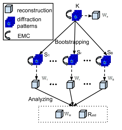
(a)

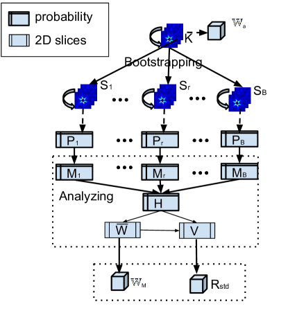
(b)

Figure 3.1. Bootstrap schemes for EMC: the standard bootstrap (left) and the EMB (right).

We now explain the EMB procedure in some detail. The EMC algorithm first runs on the whole bootstrap universe $K$, yielding $\mathbb{W}_{a}$, and saves the estimated fluence $\bar{\phi}$ at the final iteration. The EMB method then generates the bootstrap sample $(S_{r})_{r=1}^{B}$ using the same resampling method as in the standard bootstrap method described in §3.2.1. For all bootstrap samples, the EMC algorithm executes until it meets the stopping criterion (2.7), and saves the estimated rotational probabilities $(P_{jkr})_{r=1}^{B}$ for each bootstrap sample $(S_{r})_{r=1}^{B}$. Then the EMB method picks out the mode (i.e. the most probable rotation) $(M_{jkr})_{r=1}^{B}$ for each frame in the bootstrap sample,

(3.7) $$M_{jkr}=\begin{cases}1&\mbox{if}\;P_{jk^{\prime}r}=\max_{j}P_{jk^{\prime}r}\\ 0&\mbox{otherwise}\end{cases}.$$

where the $k^{\prime}$th frame of the $r$th bootstrap sample is the $k$th frame of the bootstrap universe $K$.

Following this step, EMB combines all the modes, so that each frame $K_{k}$ now comes equipped with an empirical distribution over the rotational space. The bootstrap mean of those modes is

(3.8) $$H_{jk}=\dfrac{1}{B}\sum_{r=1}^{B}M_{jkr}.$$

Using this empirical distribution, the EMB method then computes the 2D bootstrap mean as follows:

(3.9) $$\bar{W}_{ij}=\dfrac{\sum_{k}H_{jk}K_{ik}}{\sum_{k}H_{jk}\bar{\phi}_{jk}},$$

where $\bar{\phi}$ is the estimated fluence at the final iteration when reconstructing the bootstrap universe $K$.

The 2D bootstrap variance is also defined

(3.10) $$\bar{V}_{ij}=\dfrac{\sum_{k}H_{jk}(K_{ik}-\bar{\phi}_{jk}\bar{W}_{ij})^{2}}{\sum_{k}H_{jk}}.$$

To generate a comparable result to the standard bootstrap method, the EMB next compresses the bootstrap mean $\bar{W}$ and variance $\bar{V}$ by (2.6), yielding a 3D mean $\mathbb{W}_{M}$ and a 3D variance $\mathbb{V}$, respectively. The 3D standard error $R_{std}$ is again proportional to the square root of the variance (3.3).

Once all reconstructions have been obtained, the EMB method calculates the bootstrap sample bias via

(3.11) $$R_{bias} =\mathbb{W}_{M}-R\mathbb{W}_{a},$$

where $R$ is again the required rotation to align $\mathbb{W}_{a}$ to $\mathbb{W}_{M}$.

After using (3.5) to estimate the smearing error $\hat{R}_{S}$, the EMB method estimates the total reconstruction error $R_{total}$ again via (3.6).

The EMB method is summarized in Algorithm 2.

  

  Input: Initial guess of the 3D intensity, $\mathbb{W}^{(0)}$, and the bootstrap universe of diffraction patterns $K$.

  Output: Bootstrap mean $\mathbb{W}_{M}$ together with an estimated uncertainty $R_{total}$.

1:  Run the EMC algorithm on the bootstrap universe $K$, yielding $\mathbb{W}_{a}$ and the estimated fluence at the final iteration $\bar{\phi}$.

2:  Generate bootstrap samples $(S_{r})_{r=1}^{B}$ by resampling with replacement in the bootstrap universe $K$.

3:  for  $r=1,\ldots,B$ do

4:     Run the EMC algorithm on the bootstrap sample $S_{r}$ until (2.7) is satisfied, and save the probability $P_{jkr}$ at the final iteration.

5:  end for

6:  Compute the modes and the empirical distribution via (3.7) and (3.8) respectively.

7:  Calculate the 2D mean and the 2D variance by (3.9) and (3.10) respectively.

8:  Assemble the 2D mean and the 2D variance back into 3D volumes via (2.6), yielding the 3D mean $\mathbb{W}_{M}$ and the 3D variance $\mathbb{V}$.

9:  Compute the bootstrap sample bias $R_{bias}$ by (3.11) and the standard error $R_{std}$ via (3.3).

10:  Calculate the estimated smearing error $\hat{R}_{S}$ via (3.5).

11:  Estimate the total reconstruction uncertainty $R_{total}$ by (3.6).

Algorithm 2 The EMB method.

With these two bootstrap schemes, we hope to accurately estimate the algorithmic errors by reasoning essentially as in

(3.12) $$\|R_{total}\| \approx\|R_{S}\|+\|R_{T}\|+\|R_{N}\|+\|R_{F}\|$$

$$\gtrsim\|R_{S}\oplus R_{T}\oplus R_{N}\oplus R_{F}\|.$$

However, the nonlinear interaction between the various sources of uncertainty may in fact imply that $\|R_{S}\|+\|R_{T}\|+\|R_{N}\|+\|R_{F}\|<\|R_{S}\oplus R_{T}\oplus R_{N}\oplus R_{F}\|$. We usually expect that (3.12) is a robust estimate of the overall reconstruction uncertainty, at least when reconstructing a sufficiently large set of diffraction patterns.

4. Experiments

We now proceed to measure some actual algorithmic errors and assess the sharpness of our bootstrap methodology when confronted with synthetic data. In §4.1 we detail our experimental setup and in §4.2 we discuss the process of estimating the errors defined in §3. §4.3 is devoted to an investigation of the algorithmic errors and their combinations. Finally, the sharpness and robustness of the bootstrapping procedures are investigated in §4.4–4.5.

To reduce the computing time, we used our data distribution scheme described in [10] for parallelization. All implementations were compiled with GCC 4.4.7, CUDA 7.5, and Open MPI 1.8.1. With respect to the hardware, we used a cluster with 4 Nvidia Kepler GPUs in each node, interconnected via an InfiniBand 32Gbit/s fabric.

4.1. Setup and synthetic data

As summarized in §2.1, we know that a diffraction pattern is a central symmetric image containing interference of waves. The interference pattern is dependent on the rotation and shape of the target particle. To be able to discuss reproducible reconstructions, we propose the following 3D synthetic model of a 3D diffraction pattern,

(4.1) $$\centering M(\alpha,\beta,k)\@add@centering =C\sin^{2}(R(\alpha)/2)R(\alpha)^{k}+C\sin^{2}(R(\beta)/2)R(\beta)^{k},$$

(4.2) $$\centering R(\alpha)=\sqrt{\alpha_{0}X^{2}+\alpha_{1}Y^{2}+\alpha_{2}Z^{2}},\@add@centering$$

where $(X,Y,Z)$ are 3D meshgrid coordinates whose origin is the center of a $64^{3}$ cube, where 3 different grids were used in our experiments, $M_{\mbox{{\tiny grid}}}=[64^{3},128^{3},256^{3}]$, dividing the coordinates $(X,Y,Z)$ with $[1,2,4]$, respectively. Further, $k$ is the intensity drop exponent, $C$ the intensity constant, and $\alpha=(\alpha_{0},\alpha_{1},\alpha_{2})$ and $\beta=(\beta_{0},\beta_{1},\beta_{2})$ are shape vectors.

For the numerical experiments in this paper, our 3D ‘truth’ is $\mathbb{W}^{\perp}:=M(\alpha=[1.5,0.3,0.5],\beta=[0.2,0.9,1],k=-4)$. We also randomly and uniformly picked up $M_{\mbox{{\tiny data}}}=1000$ or $5000$ rotations from 400,200 rotations sampled from the 600 Cell [20, Appendix C]. With the selected rotations, we generated $M_{\mbox{{\tiny data}}}$ noiseless diffraction patterns $K^{*}$ from $\mathbb{W}^{\perp}$ via the expansion step (2.5). Using $K^{*}$, we also generated patterns sampled as a Poissonian signal $K^{0}\sim\mbox{Po}(K^{*})$, patterns with randomly varying fluence $K^{f*}=\phi K^{*}$, and the corresponding Poissonian patterns $K^{f0}\sim\mbox{Po}(\phi K^{*})$. Here, the fluence $\phi$ was uniformly and randomly chosen in $(0.9,1.2)$. All these parameters were chosen to reasonably mimic realistic conditions [4, 20].

In FXI experiments, a hole is normally located in the middle of the detector to let the unscattered X-ray photons pass, and consequentially a missing data area exists in the middle of all diffraction patterns. To make our synthetic diffraction patterns realistic, we also mask out a circular zero region, with radii $[8,16,32]$ pixels at the respective diffraction pattern sizes $M_{\mbox{{\tiny pix}}}=[64^{2},128^{2},256^{2}]$. Figure 4.1 shows the 3D ‘truth’ $\mathbb{W}^{\perp}$ with a central missing data region and a noiseless diffraction pattern.

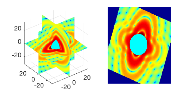
Figure 4.1. Left: Slices view of $\mathbb{W}^{\perp}:=M(\alpha=[1.5,0.3,0.5],\beta=[0.2,0.9,1],k=-4)$, as defined in (4.1). The diameter of the missing data region are $[16,32,64]$ voxels at $M_{\mbox{{\tiny grid}}}=[64^{3},128^{3},256^{3}]$. Right: A noiseless synthetic diffraction pattern generated from $\mathbb{W}^{\perp}$. Both figures are drawn in logarithmic scale.

4.2. Error metrics

Since it is reasonable to compare Fourier intensities about the same frequency, we propose a simple method to compare two 3D intensities in radial shells as follows.

Let $S=(S_{u})_{u=1}^{U}$ be the selected radial shells of a 3D intensity. The $u$th shell is given by $S_{u}=\{s=(x,y,z);s_{u}\leq\|s\|<s_{u+1}\}$, where $s$ is a point (voxel) at position $(x,y,z)$, and $\|s\|$ is the Euclidean norm.

We then define the (strong) error of the $u$th shell as follows:

(4.3) $$\hat{e}_{u}(\mathbb{W}_{1},\mathbb{W}_{2}) =\frac{1}{|S_{u}|}\sum_{s\in S_{u}}\frac{|(\mathbb{W}_{1})_{s}-(R\mathbb{W}_{2})_{s}|}{\max(\rho,(|\mathbb{W}_{1}|_{s}+|R\mathbb{W}_{2}|_{s})/2)},$$

where $\rho$ is a small cutoff number to prevent dividing by zero, and where $R$ is the rotation required to align $\mathbb{W}_{2}$ to $\mathbb{W}_{1}$. This error metric is a strong and very revealing measure, since it effectively compares relative errors in every point of $\mathbb{W}_{1}$ and $\mathbb{W}_{2}$. Alternatively, we consider a weaker version which rather compares each shell in an average sense only,

(4.4) $$e_{u}(\mathbb{W}_{1},\mathbb{W}_{2}) =\frac{\sum_{s\in S_{u}}|(\mathbb{W}_{1})_{s}-(R\mathbb{W}_{2})_{s}|}{\sum_{s\in S_{u}}|(\mathbb{W}_{1}+R\mathbb{W}_{2})_{s}|/2}.$$

In turn, we align $\mathbb{W}_{1}$ to $\mathbb{W}_{2}$ by solving the following optimization problem.

(4.5) $$\arg\min_{R}\quad U^{-1}\sum_{u=1}^{U}{e}_{u}(\mathbb{W}_{1},R\mathbb{W}_{2}),$$

that is, we find a proper alignment by minimizing the total weak error using a global optimization algorithm [26]. To be more robust, it is sometimes useful to align $\mathbb{W}_{1}$ and $\mathbb{W}_{2}$ several times from different start rotations, and pick up the mode of this sample. In practise, this minimization problem was never a major obstacle in our experiments.

In order to get a baseline for these error metrics, we now explore two basic error measurements: the 100% and the 50% hidden-data errors. Let $\mathbb{W}^{\times}$ be a reconstruction produced by inserting $M_{\mbox{{\tiny data}}}=1000$ noiseless diffraction patterns randomly into a 3D volume. Similarly, the reconstruction $\mathbb{W}^{\frac{1}{2}\times}$ is obtained by inserting the first half of those noiseless patterns randomly into a 3D volume, and the rest into the correct rotations. Comparing $\mathbb{W}^{\times}$ and $\mathbb{W}^{\frac{1}{2}\times}$ with the 3D ‘truth’ $\mathbb{W}^{\perp}$ defines 4 errors: the strong and the weak 100% errors $\hat{R}_{100}=\hat{e}(\mathbb{W}^{\times},\mathbb{W}^{\perp})$, $R_{100}=e(\mathbb{W}^{\times},\mathbb{W}^{\perp})$, and the strong and the weak 50% errors $\hat{R}_{50}=\hat{e}(\mathbb{W}^{\frac{1}{2}\times},\mathbb{W}^{\perp})$ and $R_{50}=e(\mathbb{W}^{\frac{1}{2}\times},\mathbb{W}^{\perp})$.

Figure 4.2 shows the strong and weak 100% and 50% hidden-data errors for the synthetic data model $\mathbb{W}^{\perp}:=M(\alpha=[1.5,0.3,0.5],\beta=[0.2,0.9,1],k=-4)$, from Figure 4.1. As can be seen, the strong errors ($\hat{R}_{100},\hat{R}_{50}$) are larger than their weak counterparts ($R_{100},R_{50}$), but all show the same trend. The errors rise faster at the shell distance $r:=||s||\in(30,32)$, due to the truncated domain - the regions filled with zeros on the corners of the diffraction patterns.

Based on the above, we may state that a reconstruction procedure fails if the reconstruction uncertainty is larger than $R_{100}$, or approximately when the means of the strong or, respectively, the weak errors for $r\in(8,30)$ are larger than 0.50 and 0.37. We may also claim that a proper reconstruction should generally have uncertainties less than $R_{50}$, or that the means of the strong and the weak error for $r\in(8,30)$ should be less than 0.32 and 0.23, respectively.

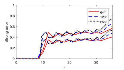
(a)

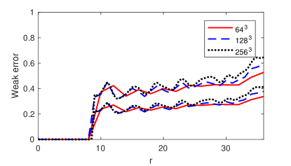
(b)

Figure 4.2. The hidden data errors at different model sizes. Left: the top three line are $\hat{R}_{100}$, and the bottom three are $\hat{R}_{50}$. Right: corresponding plots for the weak errors $R_{100}$ and $R_{50}$.

4.3. Influences of errors

In this section we investigate the algorithmic errors as defined in §3.1. Recall that the 3D ‘truth’ $\mathbb{W}^{\perp}$ and the EMC best reconstruction $\mathbb{W}^{*}$ are both used when measuring the algorithmic errors.

4.3.1. The smearing error $R_{S}$

We first measured the error that is induced by the compression step, i.e. the smearing error $R_{S}$. As defined in 3.2, $R_{S}$ compares the EMC best reconstruction $\mathbb{W}^{*}$ with the 3D ‘truth’ $\mathbb{W}^{\perp}$. We measured this error in both the strong sense $\hat{e}(\mathbb{W}^{*},R\mathbb{W}^{\perp})$ and the weak sense $e(\mathbb{W}^{*},R\mathbb{W}^{\perp})$, where $\hat{e}_{k}$ and $e_{k}$ are defined in (4.3) and (4.4), respectively.

Figure 4.3 shows these errors at the grid sizes $M_{\mbox{{\tiny grid}}}=[64^{3},128^{3},256^{3}]$. As expected, the strong error is larger and more sensitive than the weak error, but both error definitions follow a similar trend. Since linear interpolation is used for implementing both the expansion (2.5) and the compression (2.6) step, we expect and observe an overall typical $O(h^{2})$ smearing error, hence $R_{S}$ can be reduced by a factor of four by doubling the side length of the grid. Further, the $64^{3}$ resolution performs bad – the weak $R_{S}$ error is around $\frac{1}{2}R_{50}$, due to strong aliasing artifacts in the diffraction patterns.

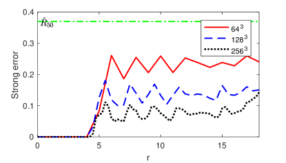
(a)

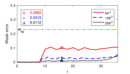
(b)

Figure 4.3. The strong (left) and the weak (right) smearing errors. The dash-dot lines are the average $R_{50}$ and $\hat{R}_{50}$, respectively.

Since the strong and the weak errors performed similarly, from now on we only present the weak error $e_{k}$ together with the average ${R}_{50}$ as a reference.

4.3.2. The hidden data and the noise error ($R_{T}$ and $R_{N}$).

We also studied the error that is induced by estimating the unobserved particles rotations - the rotational error $R_{T}$, and the error caused by noise in data - the noise error $R_{N}$.

Figure 4.4 illustrates the noise error. As expected, the noise error $R_{N}$ is small and flat, since the compression step significantly reduces the Poissonian noise by taking the average. We also observe that the noise error $R_{N}$ is positively correlated to the grid sizes $M_{\mbox{{\tiny grid}}}$ and the shell distance $r$, since the overall signal contribution per voxel decreases with $r$.

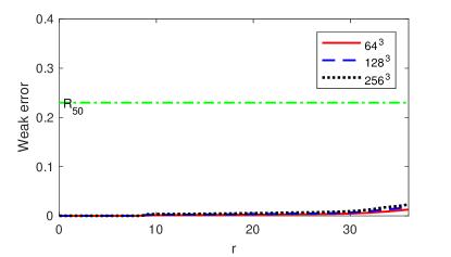
(a)

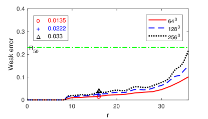
(b)

(c)

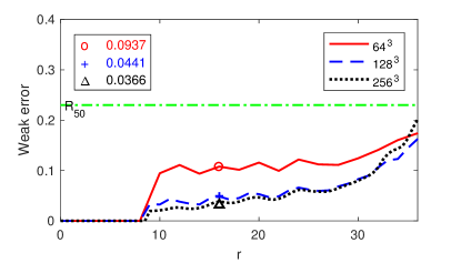
(d)

Figure 4.4. Top left: $R_{N}$, top right: $R_{T}$, bottom left: $R_{N}\oplus R_{T}$, and bottom right: $R_{S}\oplus R_{N}\oplus R_{T}$. The definitions of the errors are found in Table 3.2.

A similar analysis holds for $R_{T}$ and for $R_{N}\oplus R_{T}$, which are also positively correlated to the grid sizes $M_{\mbox{{\tiny grid}}}$ and the shell distance $r$, as shown in Figure 4.4. The rotational error $R_{T}$ increases with increasing shell distance $r$, since the error in estimating a rotational probability induces a larger contribution to total errors for voxels that are further away from the origin.

The last figure of Figure 4.4 shows the combination of the smearing, the noise, and the rotational error. As expected, this combinated error again increases with increasing shell distance $r$. However, it is negatively correlated to the grid sizes, since the smearing error $R_{S}$ reduces much quicker than the other errors increases. The $64^{3}$ resolution fails to perform well, due to the dominating smearing error.

Again, due to the artifacts of the truncated domain, all the errors investigated above increase dramatically at $r>30$.

4.3.3. The fluence error $R_{F}$ and its combinations with other errors.

Finally, we measured the error induced by the fluence estimation, i.e. the fluence error $R_{F}$, and its combinations with the other algorithmic errors. In isolation, the fluence error $R_{F}$ behaves similarly to the noise error $R_{N}$ (not shown). Figure 4.5 shows composite errors including $R_{F}$. Similar to $R_{N}\oplus R_{T}$, the combined error $R_{F}\oplus R_{N}\oplus R_{T}$ correlates positively with the grid size $M_{\mbox{{\tiny grid}}}$ and the shell distance $r$, however it is slightly larger than $R_{N}\oplus R_{T}$. Once the smearing error $R_{S}$ is considered, the $R_{S}$ error again dominates at the $64^{3}$-resolution. Further, the average of $R_{S}\oplus R_{F}\oplus R_{N}\oplus R_{T}$ at $M_{\mbox{{\tiny grid}}}=64^{3}$ and $r\in(8,30)$ is 0.22, which is just below the average ${R}_{50}$.

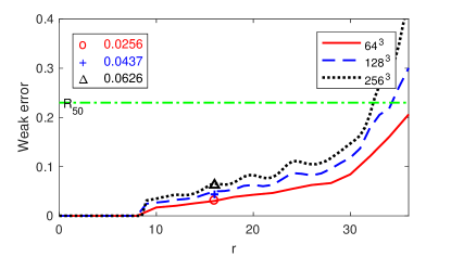
(a)

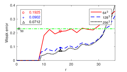
(b)

Figure 4.5. The fluence error combinations: $R_{F}\oplus R_{N}\oplus R_{T}$ (left) and $R_{S}\oplus R_{F}\oplus R_{N}\oplus R_{T}$ (right).

4.4. Sharpness of bootstrapping

In this section, we estimate the reconstruction uncertainties when the correct information: the 3D ‘truth’ $\mathbb{W}^{\perp}$, the correct fluence $\phi^{*}$, and the correct rotational probability $P^{*}$ are not accessible. We discussed both the standard bootstrap and the EMB method in detail in §3.2, where the total reconstruction uncertainty $R_{total}$ was defined in (3.6). To put $R_{total}$ in a similar form as the weak error metric (4.4), we transfer $R_{total}$ to the following radial-shell error metric:

(4.6) $$\tilde{e}_{u}(R_{total},\mathbb{W}_{a}) =\frac{\sum_{s\in S_{u}}{|R_{total}|_{s}}}{\sum_{s\in S_{u}}|\mathbb{W}_{a}|_{s}},$$

where $\mathbb{W}_{a}$ is reconstructed from the bootstrap universe.

To validate our bootstrap estimators, we used the fluence-affected Poissonian signal $K^{f0}$ as the bootstrap universe. For both bootstrap schemes, $B=100$ bootstrap samples were used, and each sample contained $M_{\mbox{{\tiny data}}}=1000$ frames.

Figure 4.6 shows the sharpness of the bootstrap estimators presented in the form of the radial-shell error metric (4.6). Comparing the results to $R_{S}\oplus R_{F}\oplus R_{N}\oplus R_{T}$ in Figure 4.5, both the standard bootstrap and the EMB method produce accurate estimations at $M_{\mbox{{\tiny grid}}}=[128^{3},256^{3}]$. However, at $M_{\mbox{{\tiny grid}}}=64^{3}$, both estimations of $R_{total}$ are smaller than $R_{S}\oplus R_{F}\oplus R_{N}\oplus R_{T}$. This is due to the underestimation of the smearing error, i.e. $R_{S}$ being much larger than the estimated smearing error $\hat{R}_{S}$ (3.5).

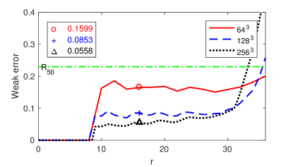
(a)

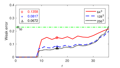
(b)

Figure 4.6. The sharpness of the bootstrap estimators in the error metric (4.6). Left: the estimated total reconstruction uncertainty $R_{total}$ calculated by the standard bootstrap estimator, and right: $R_{total}$ computed via the EMB estimator. Compare with the results in Figure 4.5.

4.5. Robustness for background noise

Other than the shot noise, the captured diffraction patterns of a typical FXI experiment might also contain artifacts of background noise, detector saturation, erroneous pixels, etc. In this section, we investigate the influence of background noise with different pattern intensities. Since the diffraction patterns are collected from the same experimental setup, it is reasonable to assume that the background noise at each pixel is approximately constant from shot to shot. Hence we sample our data as follows,

(4.7) $$K_{m}\sim\mbox{Po}(c\phi K^{*}+tK_{bg}),$$

where $K_{bg}$ is the background signal, which was measured from a real FXI single-particle experiment. If $t=1$, the so generated patterns contain added background noise. Again, $K^{*}$ stands for the noiseless patterns, and $\phi\in(0.9,1.2)$. Further, $c$ is the intensity factor that controls the total number of photons of the diffraction pattern, and set by us in order to perform the experiments.

To investigate the influences of intensity and the background noise, we generated 6 datasets without background noise and with $1000$ frames in each dataset. The intensity factors $c$ of these datasets were chosen such that the maximum number of photons in one pixel was $P_{c}=[1000,500,100,90,75,50]$ photons. We also generated their corresponding diffraction patterns with background noise. As a comparison, we generated another 6+6 datasets with the same $P_{c}$ by enlarging the number of frames to $5000$.

The standard bootstrap scheme was used to estimate the reconstruction uncertainty $R_{total}$ for each dataset via the uncertainty estimator (3.6). Again $B=100$ bootstrap samples were drawn from each dataset, and each bootstrap sample contained $M_{\mbox{{\tiny data}}}=1000$ or $5000$ diffraction patterns. Figure 4.7 (left) shows the relationship between the intensity and the average total reconstruction uncertainty for $M_{\mbox{{\tiny grid}}}=128^{3}$.

As can be seen, the background noise creates a larger reconstruction uncertainty, since the patterns with background noise violate the assumption of maximum likelihood (2.9). We also observe that the uncertainty increased with decreasing $P_{c}$, especially when $P_{c}<100$ photons. This is due to the EMC algorithm being unable to distinguish between the diffraction signals and the noise. Further, increasing the number of frames for a reconstruction reduces the total uncertainty, too.

Take a closer look at $P_{c}<100$ photons in Figure 4.7. The average uncertainty from 1000 diffraction patterns is larger than the average $R_{50}$ in Figure 4.2. We may understand this phenomenon as being roughly equivalent to a less than 50% of the hidden information being recovered from the 1000 diffraction patterns when $P_{c}$ is less than 100 photons. On the other hand, increasing the number of frames to 5000 reduces the uncertainty, and hence slightly more than 50% of the hidden information is recovered at $P_{c}=100$ photons. When $P_{c}$ is 50 photons, no reconstruction recovers more than 50% of the hidden information.

We now investigate the influence of the number of frames when the pattern signal is approximately similar to the diffraction patterns used in the 3D reconstruction of the Mimivirus [11], that is when $P_{c}=1000$. As can be seen from Figure 4.7, the average total uncertainty reduces with increasing number of frames. In order to obtain a reconstruction whose uncertainty is less than $R_{100}$, we need at least 250 diffraction patterns without background noise, or 500 frames with background noise. Further, roughly 50% of the hidden information can be obtained from 500 frames without background noise, or 750 frames with background noise.

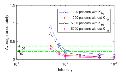
(a)

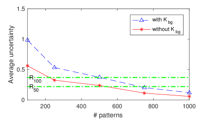
(b)

Figure 4.7. Left: The relationship between the average reconstruction uncertainty and the diffraction pattern intensity. Right: The relationship between average reconstruction uncertainty and the number of frames.

5. Conclusions

The FXI technique holds the promise of obtainining biological particle structures in a near-native state without crystallization. For the technique to become competitive with existing imaging modalities, experiment workflow as well as algorithmic developments are needed. Our aim has been to investigate the uncertainties of the reconstruction procedure.

To understand the uncertainty propagation in the EMC reconstruction procedure, we have identified several uncertainty sources and quantitatively measured the algorithmic uncertainties with the setup on synthetic data. For a 3D reconstruction coarsely resolved in the diffraction space, where fringes are close to each other, the uncertainty is high due to aliasing effects. On the other hand, the uncertainty of a more finely resolved 3D reconstruction is low, while time usage for the EMC algorithm will be high. The number of patterns required for sampling the highly resolved space is also higher. Since the uncertainty induced from the most time-consuming step of the EMC algorithm (the rotational error) is negatively correlated to the 3D reconstruction size, one can use the binned diffraction patterns to calculate the rotational probability, and use the unbinned, or the less binned patterns in the maximization step for improving the 3D reconstruction quality as well as reducing the computation time.

In order to be relevant for more realistic cases, where the biological particle structures are unknown, we have applied a bootstrap technique to the reconstruction procedure for assessing the reconstruction uncertainty. We claim that both the standard bootstrap and the EMB estimator proposed by us work well. Furthermore, in our experiments both bootstrap procedures are robust, and can tolerate the presence of non-Poissonian noise. However, we recommend to use the standard bootstrap method if the statistical model does not fit the diffraction patterns. If the diffraction patterns are extremely noisy, it is possible to modify the statistical model underlying the maximum-likelihood estimate in the M step by using a penalty function, or by directly modifying the probability distribution to account for the presence of noise photons [28, 12].

Although X-FEL science has progressed from vision to reality, and imaging techniques are improving, high-resolution 3D structures of single particles are still absent. For existing datasets, our findings indicate the benefits of using a higher number of diffraction patterns, avoiding too radical downsampling. The sampling level appropriate for proper use of EMC is higher than the Nyquist criterion on the level of oversampling necessary for 3D phase retrieval. The latter criterion is the one primarily used in previous literature discussing attainable resolution. By properly pre-processing existing datasets, more patterns usable for 3D reconstruction can probably be identified in many cases. Another option for attaining the sampling necessary would be to apply symmetry or blurring/smoothing in the compression step.

Newer facilities, such as the European XFEL, aim to increase the data rates. The European XFEL will be capable of acquiring 27,000 high-quality diffraction patterns per second - 225 times faster than the Linac Coherent Light Source (LCLS) and more than 450 times faster than the Spring-8 Ångström Compact free electron LAser (SACLA). Through an improved understanding of the uncertainty propagation properties of EMC, we hope that these future facilities will, in time, allow the 3D reconstruction of individual reproducible biological particles down to sub-nanometer resolution, with appropriate estimates of the uncertainty in those reconstructions.

References

- Antonelli M. et al. [2016] G. T. Antonelli M., B. G., et al. Fast broad-band photon detector based on quantum well devices and charge-integrating electronics for non-invasive fel monitoring. AIP Conference Proceedings, 1741, 2016. doi:10.1063/1.4952824.
- Bishop et al. [1998] C. M. Bishop, M. Svensén, and C. K. I. Williams. GTM: The generative topographic mapping. Neural Computation, 10(1):215–234, 1998. doi:10.1162/089976698300017953.
- Bogan et al. [2008] J. M. Bogan, W. H. Benner, S. Boutet, et al. Single particle X-ray diffractive imaging. Nano letters, 8(1):310–316, 2008. doi:10.1021/nl072728k.
- Bozek [2009] J. D. Bozek. AMO instrumentation for the LCLS X-ray FEL. The European Physical Journal Special Topics, 169(1):129–132, mar 2009. ISSN 1951-6355. doi:10.1140/epjst/e2009-00982-y.
- Chalupský et al. [2007] J. Chalupský, L. Juha, J. Kuba, et al. Characteristics of focused soft X-ray free-electron laser beam determined by ablation of organic molecular solids. Optics Express, 15(10):6036–6043, 2007. doi:10.1364/OE.15.006036.
- Coifman and Lafon [2006] R. R. Coifman and S. Lafon. Diffusion maps. Applied and computational harmonic analysis, 21(1):5–30, 2006. doi:10.1016/j.acha.2006.04.006.
- Dikmen and Fevotte [2012] O. Dikmen and C. Fevotte. Maximum marginal likelihood estimation for nonnegative dictionary learning in the gamma-poisson model. IEEE Transactions on Signal Processing, 60(10):5163–5175, 2012. doi:10.1109/TSP.2012.2207117.
- Efron [1979] B. Efron. Bootstrap methods: Another look at the jackknife. The Annals of Statistics, 7(1):1–26, 1979. doi:10.1214/aos/1176344552.
- Efron and Tibshirani [1994] B. Efron and R. J. Tibshirani. An introduction to the bootstrap. CRC press, 1994.
- Ekeberg et al. [2015a] T. Ekeberg, S. Engblom, and J. Liu. Machine learning for ultrafast X-ray diffraction patterns on large-scale gpu clusters. International Journal of High Performance Computing Applications, pages 233–243, 2015a. doi:10.1177/1094342015572030.
- Ekeberg et al. [2015b] T. Ekeberg, M. Svenda, C. Abergel, et al. Three-dimensional reconstruction of the giant mimivirus particle with an X-ray free-electron laser. Physical review letters, 114(9), 2015b. doi:10.1103/PhysRevLett.114.098102.
- Fessler and Rogers [1996] J. Fessler and W. Rogers. Spatial resolution properties of penalized-likelihood image reconstruction: space-invariant tomographs. IEEE Transactions on Image Processing, 5(9):1346–1358, 1996. ISSN 10577149. doi:10.1109/83.535846.
- Goodman [2005] J. W. Goodman. Introduction to Fourier Optics, chapter 4, pages 63–96. Roberts & Company Publishers, 3 edition, 2005.
- Hau-Riege et al. [2007] S. P. Hau-Riege, R. A. London, H. N. Chapman, et al. Encapsulation and diffraction-pattern-correction methods to reduce the effect of damage in X-ray diffraction imaging of single biological molecules. Physical Review Letters, 98(19):198302, 2007. doi:10.1103/PhysRevLett.98.198302.
- J D Bozek et al. [2015] L. F. J D Bozek, J C Castagna, Z. Hui, et al. X-ray split and delay device for ultrafast X-ray science at the AMO instrument at LCLS. Journal of Physics: Conference Series, 635(1):12–18, 2015. doi:10.1088/1742-6596/635/1/012018.
- Kassemeyer et al. [2012] S. Kassemeyer, J. Steinbrener, L. Lomb, et al. Femtosecond free-electron laser X-ray diffraction data sets for algorithm development. Optics Express, 20(4):4149–4158, 2012. doi:10.1364/OE.20.004149.
- Kirian R. A. et al. [2015] E. N. Kirian R. A., Awel S. et al. Simple convergent-nozzle aerosol injector for single-particle diffractive imaging with X-ray free-electron lasers. Structural Dynamics, 2(4), 2015. doi:10.1063/1.4922648.
- Lee and Seung [1999] D. D. Lee and H. S. Seung. Learning the parts of objects by non-negative matrix factorization. Nature, 401(6755):788–791, 1999. doi:10.1038/44565.
- Lee and Seung [2001] D. D. Lee and H. S. Seung. Algorithms for non-negative matrix factorization. In Advances in Neural Information Processing Systems, pages 556–562. MIT Press, 2001.
- Loh and Elser [2009] N. D. Loh and V. Elser. Reconstruction algorithm for single-particle diffraction imaging experiments. Physical Review E, 80(2):026705, 2009. doi:10.1103/PhysRevE.80.026705.
- Loh et al. [2010] N. D. Loh, M. J. Bogan, V. Elser, et al. Cryptotomography: Reconstructing 3D Fourier intensities from randomly oriented single-shot diffraction patterns. Physical Review Letters, 104:225501, 2010. doi:10.1103/PhysRevLett.104.225501.
- Maia et al. [2010] F. R. N. C. Maia, T. Ekeberg, D. van der Spoel, et al. Hawk : the image reconstruction package for coherent X-ray diffractive imaging. Journal of Applied Crystallography, 43:1535–1539, 2010. doi:10.1107/S0021889810036083.
- Neutze et al. [2000] R. Neutze, R. Wouts, D. van der Spoel, et al. Potential for biomolecular imaging with femtosecond X-ray pulses. Nature, 406(6797):752–757, 2000. doi:10.1038/35021099.
- [24] R. P. D. B. (PDB). Pdb current holdings breakdown, 6 2015. URL http://www.rcsb.org/pdb/statistics/holdings.do.
- Seibert et al. [2011] M. M. Seibert, T. Ekeberg, F. R. N. C. Maia, et al. Single mimivirus particles intercepted and imaged with an X-ray laser. Nature, 470(7332):78–81, 2011. doi:10.1038/nature09748.
- Ugray Zsolt et al. [2007] L. L. Ugray Zsolt, P. John, et al. Scatter Search and Local NLP Solvers: A Multistart Framework for Global Optimization. INFORMS J. on Computing, 19(3):328–340, 2007. doi:10.1287/ijoc.1060.0175.
- Wu [2006] X. Wu. Incorporating large unlabeled data to enhance EM classification. Journal of Intelligent Information Systems, 26(3):211–226, 2006. doi:10.1007/s10844-006-0865-3.
- Xu et al. [2010] J. Xu, K. Taguchi, and B. M. W.Tsui. Statistical Projection Completion in X-ray CT Using Consistency Conditions. IEEE Transactions on Medical Imaging, 29(8):1528–1540, aug 2010. doi:10.1109/TMI.2010.2048335.
- Yanez and Bach [2014] F. Yanez and F. R. Bach. Primal-dual algorithms for non-negative matrix factorization with the Kullback-Leibler divergence. CoRR, abs/1412.1788, 2014.
- Yang et al. [2011] Z. Yang, H. Zhang, Z. Yuan, et al. Kullback-Leibler divergence for nonnegative matrix factorization. Artificial Neural Networks and Machine Learning, pages 250–257, 2011. doi:10.1007/978-3-642-21735-7_31.
- Zribi [2010] M. Zribi. Non-parametric and region-based image fusion with bootstrap sampling. Information Fusion, 11(2):85–94, 2010. doi:10.1016/j.inffus.2008.08.004.