Gaussian intrinsic entanglement

Abstract

We introduce a cryptographically motivated quantifier of entanglement in bipartite Gaussian systems called Gaussian intrinsic entanglement (GIE). The GIE is defined as the optimized mutual information of a Gaussian distribution of outcomes of measurements on parts of a system, conditioned on the outcomes of a measurement on a purifying subsystem. We show that GIE vanishes only on separable states and exhibits monotonicity under Gaussian local trace-preserving operations and classical communication. In the two-mode case we compute GIE for all pure states as well as for several important classes of symmetric and asymmetric mixed states. Surprisingly, in all of these cases, GIE is equal to Gaussian Rényi-2 entanglement. As GIE is operationally associated to the secret-key agreement protocol and can be computed for several important classes of states it offers a compromise between computable and physically meaningful entanglement quantifiers.

Since its discovery, entanglement has transitioned from a mere paradoxical feature of quantum mechanics Einstein_35 to a powerful resource for communication and computing. The natural quest to discover all facets of entanglement revealed the need not only to verify its presence but also to quantify it. Some crucial properties of entanglement such as monogamy Coffman_00 are quantitative and therefore cannot be described without introducing entanglement measures. Further, entanglement measures are required for the characterization of entangling gates O'Brien_04 and set the bounds one has to surpass in experiments into some key quantum information protocols such as entanglement distillation Yamamoto_03 .

Existing entanglement measures either possess a good operational meaning or are computable but not both. The first kind of measure is best exemplified by the distillable entanglement Bennett_96 , which quantifies the pure-state entanglement one can distill from a shared quantum state but is difficult to compute. At the opposite extreme is the logarithmic negativity Vidal_02 ; Eisert_PhD , which is computable for any state but lacks a coherent operational interpretation. However, to assess the utility of a given entangled state in practical tasks, we need to develop entanglement measures which are both computable and physically meaningful. Unfortunately, except for the entanglement of formation Bennett_96 , which quantifies how much pure-state entanglement one needs to create a shared quantum state and which can be computed for two qubits Wootters_98 and Gaussian states Giedke_03a ; Marian_08 , no such measure is currently known.

One way to probe the gap is to quantify entanglement in the context of classical secret key agreement Maurer_93 . In this cryptographic protocol, three random variables $A,B$ and $E$ distributed according to $P(A,B,E)$ are held by two honest parties, Alice and Bob, and an adversary, Eve. Alice and Bob are connected by a public communication channel and their goal is to generate a secret key, that is a common string of random bits about which Eve has practically no information. For the key agreement to be possible it is necessary that Alice and Bob share correlations which cannot be distributed by public communication, i.e., secret correlations. A useful quantifier of secret correlations is the so called intrinsic information Maurer_99

$$I(A;B\downarrow E)=\mathop{\mbox{inf}}_{E\rightarrow\tilde{E}}[I(A;B|\tilde{E})],$$ (1)

where $I(A;B|\tilde{E})$ is the conditional mutual information and the infimum is taken over all channels $E\rightarrow\tilde{E}$. The intrinsic information is an upper bound (not always tight Renner_03 ) on the rate at which a secret key can be generated from the investigated distribution and what is more, it is conjectured that it is equal to a secret key rate in the modified key agreement protocol called public Eve scenario Christandl_04 ; PES .

The intrinsic information (1) can be used to quantify entanglement in a quantum state $\rho_{AB}$. This is accomplished by projective measurements in some bases $\{|A\rangle\}$ and $\{|B\rangle\}$, and a generalized measurement with a generating set $\{|E\rangle\}$ on subsystems $A,B$ and $E$ of a purification $|\Psi\rangle$ of the state, $\mbox{Tr}_{E}|\Psi\rangle\langle\Psi|=\rho_{AB}$. If the state $\rho_{AB}$ is entangled (separable) and the basis (set) $\{|A\rangle\}$ and $\{|B\rangle\}$ ($\{|E\rangle\}$) is chosen suitably, the obtained distribution $P(A,B,E)=|\langle A|\langle B|\langle E|\Psi\rangle|^{2}$ has strictly positive (zero) intrinsic information for any choice of the set (basis) $\{|E\rangle\}$ ($\{|A\rangle\}$ and $\{|B\rangle\}$) Gisin_00 . Thus, to faithfully map entanglement onto secret correlations the optimized intrinsic information Gisin_00 , $\mu(\rho_{AB})=\mathop{\mbox{inf}}_{\left\{|E\rangle,|\Psi\rangle\right\}}\{\mathop{\mbox{sup}}_{\left\{|A\rangle,|B\rangle\right\}}\left[I\left(A;B\downarrow E\right)\right]\}$, has to be taken, which exhibits some properties of an entanglement measure, namely equality to the von Neumann entropy on pure states and convexity. It might seem that $\mu$ is a good candidate for the sought entanglement measure but it has two drawbacks. First, it is not known whether it is non-increasing under local operations and classical communication (LOCC) as it should Vidal_00 . Second, so far it has been computed only for a two-qubit Werner state Gisin_00 .

In this Letter we propose a quantifier of bipartite entanglement called intrinsic entanglement (IE) defined as

$$E_{\downarrow}(\rho_{AB})=\mathop{\mbox{sup}}_{\left\{|A\rangle,|B\rangle\right\}}\left\{\mathop{\mbox{inf}}_{\left\{|E\rangle,|\Psi\rangle\right\}}\left[I\left(A;B\downarrow E\right)\right]\right\}.$$ (2)

The IE contains a reverse order of optimization in comparison with the quantifier $\mu$ and hence $E_{\downarrow}\leq\mu$ due to the max-min inequality Boyd_04 . The main advantage of IE is that one can compute it easier than $\mu$ as we show below. We focus on IE for an important class of Gaussian states. These states are the backbone of quantum information technologies based on continuous variables Weedbrook_12 and occur as ground or thermal state of any bosonic quantum system in a “linearized” approximation Schuch_06 . Gaussian states can be also easily prepared, manipulated and measured in many experimental platforms encompassing light, atomic ensembles, trapped ions or optomechanical systems Cerf_07 . Unfortunately, evaluation of IE for Gaussian states involves complex optimization over generally non-Gaussian measurements and states, and thus some simplifications are needed. First, we restrict Alice and Bob to Gaussian measurements. We do that because a scheme generating distribution $P$ represents the first stage of a quantum key distribution protocol (with an individual attack) and in protocols based on Gaussian states honest parties typically perform Gaussian measurements Weedbrook_12 . Second, we assume that it is optimal to use a Gaussian measurement and channel on Eve’s side. This assumption is plausible as Gaussian attacks are optimal Grosshans_04 with respect to the lower bound on the secret key rate for all important Gaussian protocols.

Here we thus investigate the so called Gaussian IE (GIE) defined by Eqs. (1) and (2), where all states, measurements and channels are Gaussian. We show that for a Gaussian state $\rho_{AB}$, the GIE is equal to the optimized mutual information of a distribution of outcomes of Gaussian measurements on subsystems $A$ and $B$ of a conditional state obtained by a Gaussian measurement on subsystem $E$ of a Gaussian purification of the state $\rho_{AB}$. Next, we prove that GIE is faithful, i.e., it vanishes iff $\rho_{AB}$ is separable, and it does not increase under Gaussian local trace-preserving operations and classical communication (GLTPOCC). Finally, we compute GIE analytically for several important classes of mixed two-mode symmetric and asymmetric Gaussian states. As the optimum in GIE is always reached by feasible homodyne and heterodyne detection, it is an experimentally meaningful quantity which stays in line with other optimized quantities such as Gaussian quantum discord Giorda_10 ; Adesso_10 ; Pirandola_14 , where the optimum is also often attained by homodyning or heterodyning. Remarkably, we find further, that the calculated GIE is always equal to an important measure of Gaussian entanglement called Gaussian Rényi-2 (GR2) entanglement Adesso_12 , which is defined as a convex roof of the pure-state Rényi-2 entropy of entanglement. The GR2 entanglement is a proper and natural measure of Gaussian entanglement being monotonic under all Gaussian LOCC (GLOCC) and monogamous. Additionally, the GR2 entanglement is additive on two-mode symmetric states and finds interpretation in terms of a phase-space sampling entropy for Wigner function Adesso_12 ; Buzek_95 . Our findings lead us to a conjecture, that GIE and GR2 entanglement are equal on all Gaussian states. If the conjecture is true, all properties of the latter quantity extend to the former and vice versa, thereby providing us with an exceptional measure of Gaussian entanglement which has cryptographic interpretation and many important properties, and which can be computed in many cases.

We consider quantum systems with infinite-dimensional Hilbert state space, e.g., light modes. An $n$-mode system is characterized by a vector of quadratures $\xi=(x_{1},p_{1},\ldots,x_{n},p_{n})^{T}$ whose components obey the canonical commutation rules $[\xi_{j},\xi_{k}]=i(\Omega_{n})_{jk}$ with $\Omega_{n}=\oplus_{j=1}^{n}i\sigma_{y}$, where $\sigma_{y}$ is the Pauli-$y$ matrix. Gaussian states are fully described by a covariance matrix (CM) $\gamma$ with entries $\gamma_{jk}=\langle\xi_{j}\xi_{k}+\xi_{k}\xi_{j}\rangle-2\langle\xi_{j}\rangle\langle\xi_{k}\rangle$ and by a vector of first moments $\langle\xi\rangle$, which is irrelevant in the present entanglement analysis and so is assumed to be zero. We use Gaussian unitary operations which are for $n$ modes represented at the level of CMs by a real $2n\times 2n$ symplectic matrix $S$ fulfilling $S\Omega_{n}S^{T}=\Omega_{n}$. We restrict ourselves to Gaussian measurements described by the positive operator valued measure Fiurasek_07

$$\Pi(d)=(2\pi)^{-n}D(d)\Pi_{0}D^{\dagger}(d),$$ (3)

which satisfies the completeness condition $\int_{\mathbb{R}_{2n}}\Pi(d){\rm d}^{2n}d=\openone$, where ${\rm d}^{2n}d=\Pi_{l=1}^{n}{\rm d}d_{l}^{(x)}{\rm d}d_{l}^{(p)}$. Here, the seed element $\Pi_{0}$ is a normalized density matrix of a generally mixed $n$-mode Gaussian state with zero first moments and CM $\Gamma$, $D(d)=\exp(-id^{T}\Omega_{n}\xi)$ is the displacement operator, and $d=(d_{1}^{(x)},d_{1}^{(p)},\ldots,d_{n}^{(x)},d_{n}^{(p)})^{T}\in\mathbb{R}_{2n}$ is a vector of measurement outcomes.

Simplification of GIE.—Initially we show that the assumption of Gaussianity of all states, measurements, and the channel $E\rightarrow\tilde{E}$, considerably simplifies the quantity (2). Assume that $\rho_{AB}\equiv\rho_{A_{1}\ldots A_{N}B_{1}\ldots B_{M}}$ of Eq.(2) is an $(N+M)$-mode Gaussian state with CM $\gamma_{AB}$. Let us further assume that $|\Psi\rangle_{ABE}$ is a Gaussian purification of the state with CM $\gamma_{\pi}$, which contains $K$ purifying modes $E_{1},E_{2},\ldots,E_{K}$. Consider now, that the subsystems $A,B$ and $E$ are distributed among Alice, Bob and Eve, who carry out local Gaussian measurements (3) characterized by covariance matrices (CMs) $\Gamma_{A},\Gamma_{B}$ and $\Gamma_{E}$, respectively. As a result, the participants share a zero-mean Gaussian distribution $P(d_{A},d_{B},d_{E})$ of measurement outcomes $d_{A},d_{B}$ and $d_{E}$ with a classical covariance matrix (CCM) CCM $\Sigma$ expressed with respect to the $AB|E$ partitioning as

$$\Sigma=\left(\begin{array}[]{cc}\gamma_{AB}+\Gamma_{A}\oplus\Gamma_{B}&\gamma_{ABE}\\ \gamma_{ABE}^{T}&\gamma_{E}+\Gamma_{E}\\ \end{array}\right)\equiv\left(\begin{array}[]{cc}\alpha&\beta\\ \beta^{T}&\delta\\ \end{array}\right),$$ (8)

where $\gamma_{AB},\gamma_{ABE}$ and $\gamma_{E}$ are blocks of the CM $\gamma_{\pi}$ according to the same partitioning. In what follows, we analyze GIE defined by Eq. (2), where the role of the distribution $P(A,B,E)$ is played by the Gaussian distribution $P(d_{A},d_{B},d_{E})$ and the optimization is performed over Gaussian channels $E\rightarrow\tilde{E}$ and CMs $\gamma_{\pi}$ and $\Gamma_{A,B,E}$.

First, we identify the conditional mutual information $I\left(A;B|E\right)$ of Eq. (1) for the distribution $P(d_{A},d_{B},d_{E})$. According to definition Cover_06 $I(A;B|E)$ is the standard mutual information $I_{c}(A;B)$ of the conditional distribution $P(d_{A},d_{B}|d_{E})$ averaged over the distribution of the variable $d_{E}$. The distribution is Gaussian with a CCM given by the Schur complement Horn_85 ; Giedke_02 of CCM (8)

$$\sigma_{AB} = \gamma_{AB}+\Gamma_{A}\oplus\Gamma_{B}-\gamma_{ABE}\frac{1}{\gamma_{E}+\Gamma_{E}}\gamma_{ABE}^{T},$$ (9)

where the inverse is to be understood generally as the pseudoinverse. Making use of the formula for mutual information of a bivariate Gaussian distribution Gelfand_57 , we arrive at $I_{c}(A;B)=f(\gamma_{\pi},\Gamma_{A},\Gamma_{B},\Gamma_{E})$, where

$$f(\gamma_{\pi},\Gamma_{A},\Gamma_{B},\Gamma_{E})=\frac{1}{2}\ln\left(\frac{\mbox{det}\sigma_{A}\mbox{det}\sigma_{B}}{\mbox{det}\sigma_{AB}}\right)$$ (10)

with $\sigma_{A,B}$ being local submatrices of CCM (9). From Eq. (10) it then follows that $I_{\rm c}(A;B)$ is independent of $d_{E}$ and hence $I(A;B|E)=I_{\rm c}(A;B)=f(\gamma_{\pi},\Gamma_{A},\Gamma_{B},\Gamma_{E})$.

We next prove that the channel $E\rightarrow\tilde{E}$ in Eq. (1) can be integrated into Eve’s measurement. Again, we assume a Gaussian channel Caruso_08 , $\tilde{d}_{E}=Xd_{E}+y$, mapping the $2K\times 1$ vector $d_{E}$ of Eve’s measurement outcomes onto a new $L\times 1$ vector $\tilde{d}_{E}$. Here $X$ is a real matrix and $y=(y_{1},y_{2},\ldots,y_{L})^{T}$ is a random vector obeying a zero mean Gaussian distribution with CCM $Y$ with elements $Y_{ij}=2\langle y_{i}y_{j}\rangle$. The channel transforms the CCM (9) to

$$\tilde{\sigma}_{AB} = \alpha-\beta X^{T}\frac{1}{X\delta X^{T}+Y}X\beta^{T},$$ (11)

where $\alpha,\beta$ and $\delta$ are blocks of CCM (8). With the help of the singular value decomposition Horn_85 of matrix $X$, CCM (11) can be recast after some algebra into the form (9) with CM $\Gamma_{E}$ replaced with a different CM (see Mista_15 for the explicit form of the new CM). Therefore, a Gaussian measurement on Eve’s system followed by a Gaussian channel on outcomes of the measurement is equivalent to another Gaussian measurement, which concludes the proof.

Further simplification follows from the invariance of CCM (9) under a change of which purification state is used, accompanied by a corresponding change to Eve’s measurement. Namely, for any two CMs $\gamma_{\pi}$ and $\bar{\gamma}_{\pi}$ of purifications with $K$-mode and $\bar{K}$-mode purifying subsystem $E$ and $\bar{E}$, where $K\leq\bar{K}$, there is a symplectic matrix on subsystem $\bar{E}$ which brings CM $\bar{\gamma}_{\pi}$ to CM $\gamma_{\pi}\oplus[\openone^{\oplus(\bar{K}-K)}]$ Mista_15 ; Giedke_03b ; Magnin_10 . As a result, for CM $\bar{\gamma}_{\pi}$ and CM $\bar{\Gamma}_{\bar{E}}$ of a measurement on subsystem $\bar{E}$, which possess CCM $\bar{\sigma}_{AB}$, Eq. (9), there is for CM $\gamma_{\pi}$ a CM $\Gamma_{E}$ of a measurement on subsystem $E$ giving $\sigma_{AB}=\bar{\sigma}_{AB}$, and vice versa Mista_15 . Accordingly, there is a free choice over which Gaussian purification of $\rho_{AB}$ to work with.

The proposed quantity GIE is defined as the conditional mutual information $I(A;B|\tilde{E})$ given in Eq. (10), where $\sigma_{AB}$ is replaced with $\tilde{\sigma}_{AB}$, Eq. (11), which is first minimized with respect to all Gaussian channels $E\rightarrow\tilde{E}$ and subsequently CMs $\Gamma_{E}$ and $\gamma_{\pi}$ of measurements and purifications, respectively, and then maximized with respect to all pure-state CMs $\Gamma_{A}$ and $\Gamma_{B}$. As any Gaussian channel can be incorporated into Eve’s measurement, we can omit the minimization with respect to the channels without loss of generality. Furthermore, as for any purification and measurement on subsystem $E$ there is a measurement on subsystem $E$ of a fixed purification giving the same conditional mutual information (10), we can further restrict ourselves in the definition of GIE to a fixed purification and minimization with respect to all CMs $\Gamma_{E}$. Consequently, GIE simplifies to

$$E_{\downarrow}^{G}\left(\rho_{AB}\right)=\mathop{\mbox{sup}}_{\Gamma_{A},\Gamma_{B}}\mathop{\mbox{inf}}_{\Gamma_{E}}f(\gamma_{\pi},\Gamma_{A},\Gamma_{B},\Gamma_{E}),$$ (12)

where $f$ is given in Eq. (10), $\gamma_{\pi}$ is CM of a fixed purification and the infimum (supremum) is taken over all CMs $\Gamma_{E}$ ($\Gamma_{A,B}$) of measurements on subsystem $E$ ($A$ and $B$).

Faithfulness.—We first prove that GIE vanishes iff $\rho_{AB}$ is separable. The proof closely follows a similar proof for intrinsic information given in Ref. Gisin_00 . The “only if” part has been proved in Ref. Mista_15 . It follows from the fact, that any separable Gaussian state has a Gaussian purification which can be projected onto a product state of subsystems $A$ and $B$ by a suitable measurement on subsystem $E$. Hence, after the measurement the CCM (9) reduces to $\sigma_{AB}=(\gamma_{A}+\Gamma_{A})\oplus(\gamma_{B}+\Gamma_{B})$ for any local Gaussian measurements on subsystems $A$ and $B$, where $\gamma_{A,B}$ denote local CMs of the product state. This implies that the mutual information (10) vanishes for any CMs $\Gamma_{A}$ and $\Gamma_{B}$, and therefore $E_{\downarrow}^{G}\left(\rho_{AB}\right)=0$ as required.

The “if” part can be proved by contradiction. Let $E_{\downarrow}^{G}\left(\rho_{AB}\right)=0$ for some entangled state $\rho_{AB}$. Then, for any CMs $\Gamma_{A}$ and $\Gamma_{B}$ there is a CM $\Gamma_{E}$ such that the mutual information in Eq. (10) vanishes. This is equivalent to the statistical independence of the variables obeying the respective bivariate Gaussian distribution with CCM $\sigma_{AB}$ Cover_06 , which implies that $\sigma_{AB}=\sigma_{A}\oplus\sigma_{B}$. Hence, for a Gaussian measurement $\Pi_{E}(d_{E})$ with CM $\Gamma_{E}$ the corresponding (unnormalized) conditional state $\mbox{Tr}_{E}[|\Psi\rangle\langle\Psi|\Pi_{E}(d_{E})]$ factorizes. By integrating the latter state over all measurement outcomes $d_{E}$ and taking into account the completeness condition for the measurement $\Pi_{E}(d_{E})$ one gets an expression of the state $\rho_{AB}$ in the form of a convex mixture of product states and therefore the state is separable, which is a contradiction. Thus, equality $E_{\downarrow}^{G}\left(\rho_{AB}\right)=0$ implies separability of $\rho_{AB}$ which accomplishes the proof.

Monotonicity.— For GIE to be a good Gaussian entanglement measure it should not increase under GLOCC Vidal_00 ; Wolf_04 . This means, that if such an operation $\mathcal{E}$ maps an input Gaussian state $\rho_{A_{\rm in}B_{\rm in}}$ onto an output Gaussian state $\rho_{A_{\rm out}B_{\rm out}}$, then

$$E_{\downarrow}^{G}\left(\rho_{A_{\rm in}B_{\rm in}}\right)\geq E_{\downarrow}^{G}\left(\rho_{A_{\rm out}B_{\rm out}}\right).$$ (13)

We here outline the proof of inequality (13) for the subset of GLOCC given by GLTPOCC (see Mista_15 for the detailed proof). First, we construct a suitable purification of the output state $\rho_{A_{\rm out}B_{\rm out}}$. For this purpose, we use realization of the operation $\cal{E}$ by a continuous-variable teleportation protocol Braunstein_98 , where a quantum channel is a Gaussian state $\chi$ representing the operation Giedke_02 ; Jamiolkowski_72 ; Fiurasek_02 (see Fig. 1(a)). Here, the input state $\rho_{A_{\rm in}B_{\rm in}}$ is teleported via input subsystems $A_{1}$ and $B_{1}$ of the state $\chi_{A_{1}B_{1}A_{2}B_{2}}$ to the output subsystems $A_{2}$ and $B_{\rm 2}$ by Bell measurements on composite subsystems $(A_{\rm in}A_{1})$ and $(B_{\rm in}B_{1})$. The measurements comprise separate measurements of the difference of the $x$-quadratures and the sum of the $p$-quadratures on each corresponding pair of modes. After the measurements and suitable displacements of subsystems $A_{2}$ and $B_{2}$, the output state $\rho_{A_{\rm out}B_{\rm out}}$ is obtained on subsystems $A_{\rm out}$ and $B_{\rm out}$. Now, by replacing states $\rho_{A_{\rm in}B_{\rm in}}$ and $\chi_{A_{1}B_{1}A_{2}B_{2}}$ with their purifications $|\Psi\rangle_{A_{\rm in}B_{\rm in}E_{\rm in}}$ and $|\chi\rangle_{A_{1}B_{1}A_{2}B_{2}E_{\chi}}$, respectively, and teleporting the respective parts of the purifications, we get the sought purification $|\Phi\rangle_{A_{\rm out}B_{\rm out}E_{\chi}E_{\rm in}}$ of the output state $\rho_{A_{\rm out}B_{\rm out}}$ (see Fig. 1(a)).

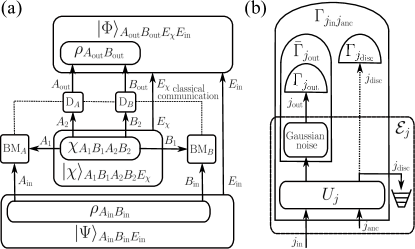
Figure 1: (a) Construction of the purification of the output state $\rho_{A_{\rm out}B_{\rm out}}$ via teleportation. $\mbox{BM}_{j}$: Bell measurement on subsystem $(j_{\rm in}j_{1})$, $\mbox{D}_{j}$: displacement of subsystem $j_{2}$. (b) Decomposition of operation $\mathcal{E}_{j}$ and its integration into a measurement.

As the operation $\mathcal{E}$ is GLTPOCC, the state $\chi$ is a Gaussian mixture of displaced Gaussian product states $\chi_{A_{1}A_{2}}(\mathbf{r})\otimes\chi_{B_{1}B_{2}}(\mathbf{r})$, where $\mathbf{r}$ characterizes the displacement, which represent products of local Gaussian trace-preserving operations Lindblad_00 ; Caruso_08 , $\mathcal{E}_{A}(\mathbf{r})\otimes\mathcal{E}_{B}(\mathbf{r})$. Consequently, we can take the purification $|\chi\rangle_{A_{1}B_{1}A_{2}B_{2}E_{\chi}}$ in the form for which there is a measurement with CM $\tilde{\Gamma}_{E_{\chi}}$ on subsystem $E_{\chi}$, which projects it onto the product states.

Let $\gamma_{\pi}^{k}$ and $\Gamma_{j_{k}}$, $j=A,B,E$, now denote CMs of the discussed purification and optimal measurements for the state $\rho_{A_{k}B_{k}}$, $k=\mathrm{in},\mathrm{out}$, i.e., $E_{\downarrow}^{G}(\rho_{{A}_{k}{B}_{k}})=f(\gamma_{\pi}^{k},\Gamma_{A_{k}},\Gamma_{B_{k}},\Gamma_{E_{k}})$. The inequality (13) is then a consequence of the following chain of inequalities:

$$E_{\downarrow}^{G}(\rho_{{A}_{\rm out}{B}_{\rm out}}) \leq f(\gamma_{\pi}^{{\rm out}},\Gamma_{A_{\rm out}},\Gamma_{B_{\rm out}},\tilde{\Gamma}_{E_{\chi}}\oplus\Gamma_{E_{\rm in}})$$

$$\leq f(\gamma_{\pi}^{{\rm in}},\tilde{\Gamma}_{A_{\rm in}},\tilde{\Gamma}_{B_{\rm in}},\Gamma_{E_{\rm in}})\leq E_{\downarrow}^{G}(\rho_{A_{\rm in}B_{\rm in}}).$$

The first inequality is satisfied because $f$ cannot decrease by replacing the optimal measurement having CM $\Gamma_{E_{\rm out}}$ by a (generally suboptimal) product measurement with CM $\tilde{\Gamma}_{E_{\chi}}\oplus\Gamma_{E_{\rm in}}$. Next, the latter measurement projects $|\chi\rangle$ onto a product state and $|\Psi\rangle_{A_{\rm in}B_{\rm in}E_{\rm in}}$ onto the state $\rho_{A_{\rm in}B_{\rm in}|E_{\rm in}}$, and hence the right-hand side of the first inequality is equal to the mutual information of outcomes of measurements with CMs $\Gamma_{A_{\rm out}}$ and $\Gamma_{B_{\rm out}}$ on the state $(\mathcal{E}_{A}\otimes\mathcal{E}_{B})(\rho_{A_{\rm in}B_{\rm in}|E_{\rm in}})$, where $\mathcal{E}_{A,B}$ are operations with zero displacements due to the independence of mutual information from displacements. Since operation $\mathcal{E}_{j}$, $j=A,B$, is trace-preserving, it can be realized by a Gaussian unitary operation $U_{j}$ on input system $j_{\rm in}$ and vacuum ancilla $j_{\rm anc}$, followed by discarding of a part of output system, $j_{\rm disc}$, and adding classical Gaussian noise Eisert_03 (see Fig. 1(b)). The noise can be integrated into a new measurement with CM $\bar{\Gamma}_{j_{\rm out}}$ and we can also work with a measurement on a larger system $(j_{\rm out}j_{\rm disc})$ with CM $\bar{\Gamma}_{j_{\rm out}}\oplus\Gamma_{j_{\rm disc}}$, because it never gives a smaller mutual information than the original measurement Cover_06 . Moreover, unitary $U_{j}$ can be integrated into a new measurement with CM $\Gamma_{j_{\rm in}j_{\rm anc}}$ on system $(j_{\rm in}j_{\rm anc})$, which yields the same mutual information which can be further rewritten in terms of some measurements with CMs $\tilde{\Gamma}_{A_{\rm in}}$ and $\tilde{\Gamma}_{B_{\rm in}}$ on state $\rho_{A_{\rm in}B_{\rm in}|E_{\rm in}}$ Mista_15 . Therefore, the second inequality holds. Finally, CMs $\tilde{\Gamma}_{A_{\rm in}}$ and $\tilde{\Gamma}_{B_{\rm in}}$ cannot give a larger mutual information than optimal CMs $\Gamma_{A_{\rm in}}$ and $\Gamma_{B_{\rm in}}$, and thus the last inequality is fulfilled, which completes the monotonicity proof.

Computability.—GIE can be calculated analytically for several classes of two-mode Gaussian states. Without loss of generality Mista_15 we can take CMs of the states in the standard form Simon_00 ; Giedke_03a

$$\gamma_{AB}=\left(\begin{array}[]{cc}a\openone&\kappa\\ \kappa&b\openone\\ \end{array}\right)$$ (16)

with $\kappa=\mbox{diag}(k_{x},-k_{p})$, where $k_{x}\geq k_{p}\geq 0$. We evaluate GIE both for symmetric states with $a=b$ as well as for some asymmetric states. First, we calculate an easier computable upper bound on GIE obtained by reversing the order of optimization in its definition (12). Next, we find for some fixed measurements on modes $A$ and $B$ a measurement on subsystem $E$ giving minimal $f$ which at the same time saturates the bound (see Appendix SI for details). It turns out, that for all symmetric (asymmetric) states considered here, GIE is achieved by double homodyne detection on modes $A$ and $B$, and homodyne detection (heterodyne detection, i.e., projection onto coherent states) on subsystem $E$. We have found GIE for the following three sets of states:

(i) Symmetric GLEMS Adesso_04 .— The states $(\equiv\rho_{AB}^{(1)})$ have one unit symplectic eigenvalue Williamson_36 whence $k_{x}=a-1/(a+k_{p})$ and a subsystem $E$ is single-mode. For all the states GIE reads as SI

$$E_{\downarrow}^{G}\left(\rho_{AB}^{(1)}\right)=\ln\left(\frac{a}{\sqrt{a^{2}-k_{p}^{2}}}\right).$$ (17)

If $k_{x}=k_{p}$ symmetric GLEMS satisfy $a^{2}-k_{p}^{2}=1$ and therefore they reduce to pure states $(\equiv\rho_{AB}^{p})$. Equation (17) then gives $E_{\downarrow}^{G}(\rho_{AB}^{p})=\ln(a)$ Mista_15 .

(ii) Symmetric squeezed thermal states Botero_03 .—The states $(\equiv\rho_{AB}^{(2)})$ fulfil the condition $k_{x}=k_{p}\equiv k$ and they are entangled iff $a-k<1$ Simon_00 ; Giedke_03a . For all the entangled states which satisfy $a\leq 2.41$ GIE is equal to SI

$$E_{\downarrow}^{G}\left(\rho_{AB}^{(2)}\right)=\ln\left[\frac{(a-k)^{2}+1}{2(a-k)}\right],$$ (18)

whereas for separable states $E_{\downarrow}^{G}(\rho_{AB}^{(2)})=0$ by faithfulness.

(iii) Asymmetric squeezed thermal GLEMS.—The states $(\equiv\rho_{AB}^{(3)})$ fulfill the condition $k_{x}=k_{p}\equiv k$ and possess one unit symplectic eigenvalue. For all the states for which $\sqrt{ab}\leq 2.41$ GIE is given by SI

$$E_{\downarrow}^{G}\left(\rho_{AB}^{(3)}\right)=\ln\left(\frac{a+b}{|a-b|+2}\right).$$ (19)

Discussion and conclusions.— We have proposed a quantifier of Gaussian entanglement GIE which compromises between computability and operational significance. Closed formulae for GIE for two classes of symmetric states have been obtained, Eqs. (17) and (18), which can be compactly written as $E_{\downarrow}^{G}(\rho_{AB})=\ln\{[\tilde{\nu}_{-}+(\tilde{\nu}_{-})^{-1}]/2\}$ if $\tilde{\nu}_{-}<1$ and $E_{\downarrow}^{G}(\rho_{AB})=0$ if $\tilde{\nu}_{-}\geq 1$, where $\tilde{\nu}_{-}=\sqrt{(a-k_{x})(a-k_{p})}$. Interestingly, this is nothing but GR2 entanglement for symmetric states Adesso_12 ; Giedke_03a . As the GIE for some asymmetric states, Eq. (19), also coincides with the GR2 entanglement SI we conjecture, that the two quantities are equivalent. The confirmation or refutation of the conjecture as well as analysis of the other properties of GIE is left for future research. We hope that the present results will stimulate further studies of physically meaningful computable entanglement measures.

We would like to thank J. Fiurášek and G. Adesso for fruitful discussions. L. M. acknowledges the Project No. P205/12/0694 of GAČR.

Appendix A GIE for two-mode Gaussian states

For a Gaussian state $\rho_{AB}$ of two modes $A$ and $B$ GIE is defined explicitly as

$$E_{\downarrow}^{G}\left(\rho_{AB}\right)=\mathop{\mbox{sup}}_{\Gamma_{A},\Gamma_{B}}\mathop{\mbox{inf}}_{\Gamma_{E}}f\left(\gamma_{\pi},\Gamma_{A},\Gamma_{B},\Gamma_{E}\right),$$ (20)

where

$$f\left(\gamma_{\pi},\Gamma_{A},\Gamma_{B},\Gamma_{E}\right)=\frac{1}{2}\ln\left(\frac{\mbox{det}\sigma_{A}\mbox{det}\sigma_{B}}{\mbox{det}\sigma_{AB}}\right)$$ (21)

with

$$\sigma_{AB} = \gamma_{AB|E}+\Gamma_{A}\oplus\Gamma_{B},$$ (22)

where $\sigma_{A,B}$ are local submatrices of $\sigma_{AB}$ and $\Gamma_{A}$ and $\Gamma_{B}$ are single-mode CMs of Gaussian measurements on modes $A$ and $B$, respectively. Here,

$$\gamma_{AB|E} = \gamma_{AB}-\gamma_{ABE}\frac{1}{\gamma_{E}+\Gamma_{E}}\gamma_{ABE}^{T}$$ (23)

is a CM of a conditional state $\rho_{AB|E}$ Giedke_02 of modes $A$ and $B$ obtained by a Gaussian measurement with CM $\Gamma_{E}$ on purifying subsystem $E$ of the minimal purification Caruso_11 of the state $\rho_{AB}$, where $\gamma_{AB}$ is a CM of the state $\rho_{AB}$ and $\gamma_{ABE}$ and $\gamma_{E}$ denote the blocks of the CM of the purification $(\equiv\gamma_{\pi})$ expressed with respect to the $AB|E$ splitting, i.e.,

$$\gamma_{\pi}=\left(\begin{array}[]{cc}\gamma_{AB}&\gamma_{ABE}\\ \gamma_{ABE}^{T}&\gamma_{E}\\ \end{array}\right).$$ (26)

If the Gaussian state $\rho_{AB}$ is a pure state ($\equiv\rho^{p}$), the off-diagonal block $\gamma_{ABE}$ is a zero matrix and the GIE then can be calculated easily. In the main text as well as in Ref. Mista_15 it was shown, that in this case the GIE coincides with the Gaussian Rényi-2 (GR2) entanglement ($\equiv E_{2}^{G}(\rho^{p})$) Adesso_12 ,

$$E_{\downarrow}^{G}\left(\rho^{p}\right)=E_{2}^{G}\left(\rho^{p}\right)=\frac{1}{2}\ln\left(\mbox{det}\gamma_{A}\right),$$ (27)

where $\gamma_{A}$ is a CM of the reduced state of mode $A$ of the state $\rho^{p}$.

In what follows, we focus on calculation of GIE for mixed two-mode Gaussian states. The states possess the blocks $\gamma_{ABE}$ and $\gamma_{E}$ of the form Mista_15

$$\gamma_{ABE}=S^{-1}\gamma_{ABE}^{(0)},\quad\gamma_{E}=\gamma_{E}^{(0)},$$ (28)

where

$$\gamma_{ABE}^{(0)}=\left(\begin{array}[]{c}\bigoplus_{i=1}^{R}\sqrt{\nu_{i}^{2}-1}\sigma_{z}\\ \mathbb{O}_{2(2-R)\times 2R}\\ \end{array}\right),\quad\gamma_{E}^{(0)}=\bigoplus_{i=1}^{R}\nu_{i}\openone.$$ (31)

Here $\sigma_{z}=\mbox{diag}(1,-1)$ is the diagonal Pauli-$z$ matrix, $\mathbb{O}_{I\times J}$ is the $I\times J$ zero matrix, $\openone$ is the $2\times 2$ identity matrix and $S$ is a symplectic matrix, i.e., a $4\times 4$ real matrix satisfying the symplectic condition

$$S\Omega S^{T}=\Omega,$$ (32)

where

$$\Omega=\bigoplus_{i=1}^{2}J,\quad J=\left(\begin{array}[]{cc}0&1\\ -1&0\\ \end{array}\right),$$ (33)

that brings the CM $\gamma_{AB}$ to the Williamson normal form Williamson_36

$$S\gamma_{AB}S^{T}=\mbox{diag}(\nu_{1},\nu_{1},\nu_{2},\nu_{2}).$$ (34)

Here $\nu_{1}\geq\nu_{2}\geq 1$ are the so called symplectic eigenvalues of CM $\gamma_{AB}$ and $R=1,2$ is the number of the symplectic eigenvalues strictly greater than one. The use of Eq. (28) on the right-hand side (RHS) of Eq. (23) further yields for the CM $\gamma_{AB|E}$ the expression

$$\gamma_{AB|E}=S^{-1}\gamma_{AB|E}^{(0)}(S^{-1})^{T}$$ (35)

with

$$\gamma_{AB|E}^{(0)} = \gamma_{AB}^{(0)}-\gamma_{ABE}^{(0)}\frac{1}{\gamma_{E}^{(0)}+\Gamma_{E}}(\gamma_{ABE}^{(0)})^{T},$$ (36)

where $\gamma_{AB}^{(0)}$ denotes the Williamson normal form (34) of CM $\gamma_{AB}$, i.e., $\gamma_{AB}^{(0)}=\mbox{diag}(\nu_{1},\nu_{1},\nu_{2},\nu_{2})$.

In order to calculate the GIE we now need to express CM (36) as well as the symplectic matrix $S$ appearing in Eq. (35) in terms of the elements of the CM $\gamma_{AB}$. For this purpose it is convenient to express the CM in a block form with respect to the $A|B$ splitting,

$$\gamma_{AB}=\left(\begin{array}[]{cc}A&C\\ C^{T}&B\\ \end{array}\right).$$ (39)

Owing to the invariance of GIE (20) under the Gaussian local unitary operations Mista_15 we can without loss of generality assume CM (39) to be in the standard form Simon_00 ,

$$\gamma_{AB}=\left(\begin{array}[]{cccc}a&0&c_{x}&0\\ 0&a&0&c_{p}\\ c_{x}&0&b&0\\ 0&c_{p}&0&b\\ \end{array}\right)$$ (44)

with $c_{x}\geq|c_{p}|\geq 0$. Since states with $c_{x}c_{p}\geq 0$ are separable Simon_00 and thus possess zero GIE Mista_15 , in calculations we can restrict ourself only to CMs satisfying $c_{x}c_{p}<0$. Introducing new more convenient parameters $k_{x}\equiv c_{x}$ and $k_{p}\equiv|c_{p}|=-c_{p}$, we arrive at the following standard-form CM which we shall consider in what follows Giedke_03a :

$$\gamma_{AB}=\left(\begin{array}[]{cccc}a&0&k_{x}&0\\ 0&a&0&-k_{p}\\ k_{x}&0&b&0\\ 0&-k_{p}&0&b\\ \end{array}\right),$$ (49)

where $k_{x}\geq k_{p}>0$.

The symplectic eigenvalues of CM (49) can be calculated conveniently from the eigenvalues of the matrix $i\Omega\gamma_{AB}$ which are of the form $\{\pm\nu_{1},\pm\nu_{2}\}$ Vidal_02 . In terms of parameters $a,b,k_{x}$ and $k_{p}$ they read explicitly as

$$\nu_{1,2}=\sqrt{\frac{\Delta\pm\sqrt{D}}{2}},$$ (50)

where

$$\Delta = a^{2}+b^{2}-2k_{x}k_{p},$$

$$D = \Delta^{2}-4\mbox{det}\gamma_{AB}$$

$$= \left(a^{2}-b^{2}\right)^{2}+4\left(ak_{x}-bk_{p}\right)\left(bk_{x}-ak_{p}\right).$$

Similarly, we can express the symplectic matrix $S$ which brings CM (49) to Williamson normal form (34) in terms of parameters $a,b,k_{x}$ and $k_{p}$. This can be done using either a method of Ref. Serafini_05 or a method of Ref. Pirandola_09 . For a generic two-mode CM (49) the form of the matrix $S$ is complex and therefore we do not write it here explicitly. In what follows, we work with particular subclasses of the class of generic two-mode Gaussian states for which $S$ attains a simple form which is presented explicitly in the respective subsection.

Appendix B GIE for symmetric states

In this section we calculate GIE defined in Eq. (8) of the main text for some subclasses of the class of two-mode symmetric Gaussian states. The states are characterized by the condition $a=b$ whence their standard-form CMs (44) and (49) reduce to

$$\gamma_{AB}=\left(\begin{array}[]{cccc}a&0&c_{x}&0\\ 0&a&0&c_{p}\\ c_{x}&0&a&0\\ 0&c_{p}&0&a\\ \end{array}\right)$$ (56)

and

$$\gamma_{AB}=\left(\begin{array}[]{cccc}a&0&k_{x}&0\\ 0&a&0&-k_{p}\\ k_{x}&0&a&0\\ 0&-k_{p}&0&a\\ \end{array}\right),$$ (61)

respectively. For the sake of further use let us also recap here that the matrix (61) describes a CM of a physical quantum state if and only if $a^{2}-k_{x}^{2}\geq 1$ and that the CM corresponds to an entangled state if and only if $1>(a-k_{x})(a-k_{p})$ Giedke_03a .

From Eq. (50) it further follows that the symplectic eigenvalues of CM (61) read explicitly as

$$\nu_{1} = \sqrt{\left(a+k_{x}\right)\left(a-k_{p}\right)},$$

$$\nu_{2} = \sqrt{\left(a-k_{x}\right)\left(a+k_{p}\right)}.$$ (62)

As for the symplectic matrix $S$, we calculate it using the method of Ref. Serafini_05 . Here, we seek the matrix in the form of a product $S=\left(\oplus_{i=1}^{2}V^{\ast}\right)W^{T}$, where

$$V=\frac{1}{\sqrt{2}}\left(\begin{array}[]{cc}i&-i\\ 1&1\\ \end{array}\right)$$ (63)

and $W$ contains in its columns the eigenvectors of the matrix $i\Omega\gamma_{AB}$ which are chosen such that $S$ is real, it satisfies the symplectic condition (32) and it does not mix position and momentum quadratures. Thus we find the symplectic matrix $S$ that brings the CM (61) to the Williamson normal form (34) to be the following product

$$S=(S_{A}\oplus S_{B})U_{BS}.$$ (64)

Here,

$$U_{BS}=\frac{1}{\sqrt{2}}\left(\begin{array}[]{cc}\openone&\openone\\ -\openone&\openone\\ \end{array}\right)$$ (65)

is a matrix describing a balanced beam splitter and

$$S_{A}=\left(\begin{array}[]{cc}z_{A}^{-1}&0\\ 0&z_{A}\\ \end{array}\right),\quad S_{B}=\left(\begin{array}[]{cc}z_{B}&0\\ 0&z_{B}^{-1}\\ \end{array}\right)$$ (66)

with $z_{A}=\sqrt[4]{\frac{a+k_{x}}{a-k_{p}}}>1$ and $z_{B}=\sqrt[4]{\frac{a+k_{p}}{a-k_{x}}}>1$ are matrices corresponding to local squeezing transformations in quadratures $x_{A}$ and $p_{B}$, respectively.

Making use of the symplectic eigenvalues (B) and the symplectic matrix (64) we can now express CM (35) solely in terms of the parameters $a,k_{x}$ and $k_{p}$ and the CM $\Gamma_{E}$. However, this form of CM (35) is not suitable for analytical calculation of the GIE, because the CM depends on CM $\Gamma_{E}$ that we minimize over in the definition of GIE, Eq. (20), in a complicated way via the term $\frac{1}{\gamma_{E}^{(0)}+\Gamma_{E}}$. Although the term can be calculated explicitly for an arbitrary two-mode Gaussian state, the obtained form of CM (36) still depends on elements of CM $\Gamma_{E}$ in a way which is too complicated for analytical calculations. Nevertheless, there are some subclasses of the set of symmetric states for which the CM simplifies such that the GIE can be calculated analytically. These states can be identified if one realizes that the dimension of CM $\gamma_{E}^{(0)}$ and therefore also CM $\Gamma_{E}$ is determined by the number $R$, which appears in Eq. (31) and which denotes the number of symplectic eigenvalues of a respective two-mode Gaussian state which are strictly greater than one. Therefore, the set of mixed two-mode Gaussian states splits into two subsets containing states with $R=1$ and $R=2$, respectively. States with $R=1$ are more simple because for them the matrix $\gamma_{E}^{(0)}+\Gamma_{E}$ is just single-mode and therefore the inverse $\frac{1}{\gamma_{E}^{(0)}+\Gamma_{E}}$ is simple. In the following subsection we show, that for symmetric states with $R=1$ the GIE can be calculated analytically. The next subsection is then dedicated to analytical evaluation of GIE for a subclass of more complicated symmetric states with $R=2$. Specifically, in this subsection we calculate GIE for a subclass of the symmetric states satisfying $\nu_{1}=\nu_{2}$ Botero_03 , which are the so called symmetric squeezed thermal states.

B.1 GIE for symmetric GLEMS

Let us consider a two-mode Gaussian state $\rho_{AB}^{(1)}$ with a CM $\gamma_{AB}^{(1)}$ and $R=1$. Since $\nu_{2}=1$ holds for this state it is a Gaussian state with a partial minimal uncertainty. This state is also known to be the Gaussian least entangled state for given global and local purities (GLEMS) Adesso_04 and it possesses the other symplectic eigenvalue equal to

$$\nu\equiv\nu_{1}=\sqrt{\mbox{det}\gamma_{AB}^{(1)}}$$ (67)

as can be seen from Eq. (34). Because $R=1$, the minimal purification of GLEMS contains only a single purifying mode $E$ and therefore also the CM $\Gamma_{E}$ appearing in CM (36) is single-mode.

Let us assume now the CM in the form $\Gamma_{E}=P(\varphi)\mbox{diag}(V_{x},V_{p})P^{T}(\varphi)$, where

$$P(\varphi)=\left(\begin{array}[]{cc}\cos\varphi&-\sin\varphi\\ \sin\varphi&\cos\varphi\\ \end{array}\right)$$ (68)

with $\varphi\in[0,\pi)$, $V_{x}=\tau e^{2t}$ and $V_{p}=\tau e^{-2t}$, where $\tau\geq 1$ and $t\geq 0$. Using relation $P^{T}(\varphi)=\sigma_{z}P(\varphi)\sigma_{z}$ one gets after some algebra that the CM (35) can be expressed as

$$\gamma_{AB|E}^{(1)}=S^{-1}\left[\gamma_{A|E}(\nu)\oplus\openone_{B}\right](S^{-1})^{T}.$$ (69)

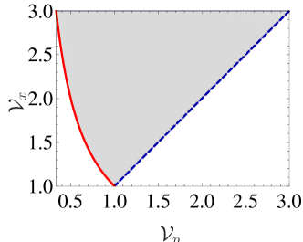
Figure 2: (Color online) An example of the set $\mathscr{M}$ (gray area) for $\nu=3$. Solid red curve and dashed blue curve depict the boundary curves $\mathcal{V}_{x}=1/\mathcal{V}_{p}$ and $\mathcal{V}_{x}=\mathcal{V}_{p}$, respectively.

Here,

$$\gamma_{A|E}(\nu)=P^{T}(\varphi)\mbox{diag}(\mathcal{V}_{x},\mathcal{V}_{p})P(\varphi),$$ (70)

where

$$\mathcal{V}_{x}=\frac{\nu V_{x}+1}{\nu+V_{x}},\quad\mathcal{V}_{p}=\frac{\nu V_{p}+1}{\nu+V_{p}}$$ (71)

are the eigenvalues of the CM. From the definition of parameters $V_{x}$ and $V_{p}$ given below Eq. (68) it then follows that $V_{x}\geq 1$, $V_{x}\geq V_{p}\geq 0$ and $V_{x}V_{p}\geq 1$. Consequently, at given $\nu$ the eigenvalues (71) lie in the subset $\mathscr{M}$ of the $(\mathcal{V}_{p},\mathcal{V}_{x})$-plane such that if $\mathcal{V}_{p}\in[1/\nu,1]$ then $\mathcal{V}_{x}\in[1/\mathcal{V}_{p},\nu]$, whereas if $\mathcal{V}_{p}\in(1,\nu]$ then $\mathcal{V}_{x}\in[\mathcal{V}_{p},\nu]$ (see Fig. 2).

For symmetric GLEMS we can further insert for the symplectic matrix $S$ on the RHS of Eq. (69) the decomposition (64) which yields

$$\gamma_{AB|E}^{(1)}=U_{BS}^{T}\left[S_{A}^{-1}\gamma_{A|E}(\nu)(S_{A}^{-1})^{T}\oplus\gamma_{B}^{\rm sq}\right]U_{BS},$$ (72)

where $\gamma_{B}^{\rm sq}=S_{B}^{-1}(S_{B}^{-1})^{T}=\mbox{diag}(z_{B}^{-2},z_{B}^{2})$, and where we have used the orthogonality of the matrix (65).

The form of CM (72) is now suitable for carrying out of the last step of calculation of GIE, Eq. (20), which is the optimization of the function (21) with respect to CMs $\Gamma_{A},\Gamma_{B}$ and $\Gamma_{E}$. Here, we perform the optimization by means of the method, which was used in Ref. Mista_15 for calculation of the GIE for a particular instance of symmetric GLEMS given by the two-mode reduction of the three-mode continuous-variable (CV) Greenberger-Horne-Zeilinger (GHZ) state Loock_00 . In this method, we calculate the GIE for a Gaussian state $\rho_{AB}^{(1)}$ in two steps. First, we calculate an easier computable upper bound

$$U\left(\rho_{AB}^{(1)}\right)\equiv\mathop{\mbox{inf}}_{\Gamma_{E}}\mathop{\mbox{sup}}_{\Gamma_{A},\Gamma_{B}}f(\gamma_{\pi},\Gamma_{A},\Gamma_{B},\Gamma_{E})$$ (73)

on GIE, $E_{\downarrow}^{G}(\rho_{AB}^{(1)})\leq U(\rho_{AB}^{(1)})$. In the second step, we find for particular fixed CMs $\Gamma_{A}$ and $\Gamma_{B}$ an optimal CM $\tilde{\Gamma}_{E}$ which minimizes $f(\gamma_{\pi},\Gamma_{A},\Gamma_{B},\Gamma_{E})$, i.e., $f(\gamma_{\pi},\Gamma_{A},\Gamma_{B},\tilde{\Gamma}_{E})=\mathop{\mbox{inf}}_{\Gamma_{E}}f(\gamma_{\pi},\Gamma_{A},\Gamma_{B},\Gamma_{E})$, and which at the same time saturates the upper bound, i.e., $U(\rho_{AB}^{(1)})=f(\gamma_{\pi},\Gamma_{A},\Gamma_{B},\tilde{\Gamma}_{E})$. As a consequence, the GIE for state $\rho_{AB}^{(1)}$ then reads as

$$E_{\downarrow}^{G}\left(\rho_{AB}^{(1)}\right)=f(\gamma_{\pi},\Gamma_{A},\Gamma_{B},\tilde{\Gamma}_{E}).$$ (74)

In order to calculate the upper bound (73), we first calculate the quantity

$$\mathcal{I}_{c}^{G}\left(\rho_{AB|E}^{(1)}\right)\equiv\mathop{\mbox{sup}}_{\Gamma_{A},\Gamma_{B}}f(\gamma_{\pi},\Gamma_{A},\Gamma_{B},\Gamma_{E}),$$ (75)

which is the Gaussian classical mutual information (GCMI) of the conditional quantum state $\rho_{AB|E}^{(1)}$ with CM (72) Mista_11 . Substituting on the RHS of Eq. (72) for the matrix $U_{BS}$ from Eq. (65) one finds, that the block form with respect to the $A|B$ splitting of CM (72) reads as

$$\gamma_{AB|E}^{(1)}=\left(\begin{array}[]{cc}A&C\\ C&A\\ \end{array}\right)$$ (78)

and therefore the CM is symmetric under the exchange of modes $A$ and $B$. This implies, that the standard form of CM (72) attains the symmetric form (56). Denoting now the parameters of the standard form as $\tilde{a},\tilde{c}_{x}$ and $\tilde{c}_{p}$ we can use the result of Ref. Mista_15 to calculate the quantity (75). Specifically, in Ref. Mista_15 it was shown, that for states with the symmetric standard-form CM where the parameters $\tilde{a}$ and $\tilde{c}_{x}$ satisfy inequality

$$2+\frac{1}{\tilde{a}}-\tilde{s}\geq 0,$$ (79)

where $\tilde{s}\equiv\sqrt{\tilde{a}^{2}-\tilde{c}_{x}^{2}}$, the GCMI (75) is attained by homodyne detections of quadratures $x_{A}$ and $x_{B}$ on modes $A$ and $B$, for which it is of the form:

$$\mathcal{I}_{c}^{G}\left(\rho_{AB|E}^{(1)}\right)=\frac{1}{2}\ln\frac{\tilde{a}^{2}}{\tilde{a}^{2}-\tilde{c}_{x}^{2}}=-\ln\sqrt{1-g^{2}},$$ (80)

where $g\equiv\tilde{c}_{x}/\tilde{a}$. By calculating explicitly the blocks $A$ and $C$ of CM (78) we can express the quantities $\tilde{a}$ and $g$ in terms of the parameters $a,k_{x}$ and $k_{p}$ of the original state and the variables $\mathcal{V}_{p},\mathcal{V}_{x}$ and $\varphi$ over which we carry out minimization. Making use of the formula $\tilde{a}=\sqrt{\mbox{det}A}$ one finds that

$$\tilde{a}=\frac{\sqrt{1+\mathcal{V}_{x}\mathcal{V}_{p}+2[\mathcal{V}_{+}\cosh(2q)+\mathcal{V}_{-}\sinh(2q)\cos(2\varphi)]}}{2},$$

where $\mathcal{V}_{\pm}=(\mathcal{V}_{x}\pm\mathcal{V}_{p})/2$ and $q=\ln(z_{A}z_{B})$, whereas for the quantity $g$ one gets Mista_15

$$g=\frac{\mathcal{K}}{\tilde{a}^{2}}+\sqrt{\left(\frac{\mathcal{K}}{\tilde{a}^{2}}-1\right)^{2}-\frac{1}{\tilde{a}^{2}}}$$ (82)

with $\mathcal{K}=(\mathcal{V}_{x}\mathcal{V}_{p}-1)/4$.

For calculation of the upper bound (73) it remains to minimize the RHS of Eq. (80) over all 3-tuples $(\mathcal{V}_{p},\mathcal{V}_{x},\varphi)$ belonging to the Cartesian product $\mathscr{O}=\mathscr{M}\times[0,\pi)$, where the set $\mathscr{M}$ is defined below equation (71). This amounts to the minimization of the RHS of Eq. (82) on the set $\mathscr{O}$, which can be performed exactly as in Ref. Mista_15 . Namely, comparison of the quantities (B.1) and (82) with the same quantities for the CV GHZ state analyzed in Ref. Mista_15 reveals, that they are exactly the same. The only difference is in the parameter $q$ which is for the present case defined below Eq. (B.1), whereas for the CV GHZ state it is equal to $q=r+\ln(\sqrt{x_{-}/x_{+}})/2$ with $x_{\pm}=(e^{\pm 2r}+2e^{\mp 2r})/3$, where $r\geq 0$ is a squeezing parameter. Minimizing therefore the quantity $g$, Eq. (82), exactly as in Ref. Mista_15 and restricting ourselves only to entangled states satisfying the necessary and sufficient condition for entanglement, $1>(a-k_{x})(a-k_{p})$, one finds, that the quantity possesses three candidates for the minimum which lie on the edges of the volume $\mathscr{O}$ and correspond to:

1. Homodyne detection of quadrature $p_{E}$ on mode $E$, i.e., $\Gamma_{E}=\Gamma_{p}^{t\rightarrow+\infty}$, where $\Gamma_{p}^{t}\equiv\mbox{diag}(e^{2t},e^{-2t})$, or discarding of mode $E$, which yields

$$U_{1}\left(\rho_{AB}^{(1)}\right)=\ln\left(a\sqrt{\frac{a+k_{p}}{a+k_{x}}}\right)=\ln\left(\frac{a}{\sqrt{a^{2}-k_{x}^{2}}}\right).$$

Here, the second equality is a consequence of the equality

$$a+k_{p}=\frac{1}{a-k_{x}},$$ (84)

which follows from the defining equality for symmetric GLEMS, $\nu_{2}=\sqrt{(a-k_{x})(a+k_{p})}=1$.

2. Heterodyne detection on mode $E$, i.e., $\Gamma_{E}=\openone$, which gives

$$U_{2}\left(\rho_{AB}^{(1)}\right)=\ln\left[\frac{1}{2}\left(z_{A}z_{B}+\frac{1}{z_{A}z_{B}}\right)\right],$$ (85)

where the parameters $z_{A}$ and $z_{B}$ are defined below Eq. (66).

3. Homodyne detection of quadrature $x_{E}$ on mode $E$, i.e., $\Gamma_{E}=\Gamma_{x}^{t\rightarrow+\infty}$, where $\Gamma_{x}^{t}\equiv\mbox{diag}(e^{-2t},e^{2t})$, for which the upper bound (73) is equal to

$$U_{3}\left(\rho_{AB}^{(1)}\right)=\ln\left(a\sqrt{\frac{a-k_{x}}{a-k_{p}}}\right)=\ln\left(\frac{a}{\sqrt{a^{2}-k_{p}^{2}}}\right).$$

Comparison of the upper bounds (B.1), (85) and (B.1) shows that $U_{1}\geq U_{3}$ and $U_{2}\geq U_{3}$ and therefore, the upper bound (73) is equal to $U_{3}$, i.e., $U(\rho_{AB}^{(1)})=U_{3}(\rho_{AB}^{(1)})$. Because the bound also represents at homodyne detections of quadratures $x_{A}$ and $x_{B}$ on modes $A$ and $B$, the least mutual information over all Gaussian measurements on mode $E$, the upper bound (B.1) also gives GIE for all symmetric GLEMS satisfying inequality (79),

$$E_{\downarrow}^{G}\left(\rho_{AB}^{(1)}\right)=\ln\left(\frac{a}{\sqrt{a^{2}-k_{p}^{2}}}\right).$$ (87)

Note, that the RHS of the latter formula is nothing but the mutual information of the joint distribution of outcomes of measurements of quadratures $p_{A}$ and $p_{B}$ on a symmetric Gaussian state with CM (61).

In particular, for the CV GHZ state we have

$$a=\sqrt{x_{+}x_{-}},\quad k_{x,p}=\sqrt{\frac{x_{\mp}}{x_{\pm}}}(x_{-}-x_{+})$$ (88)

which gives after substitution into the RHS of Eq. (87) the formula

$$E_{\downarrow}^{G}\left(\rho_{AB}^{GHZ}\right)=\ln\left(\frac{x_{-}}{e^{r}\sqrt{x_{+}}}\right).$$ (89)

The latter expression agrees with the GIE for the CV GHZ state derived in Ref. Mista_15 .

It remains to identify the set of symmetric entangled GLEMS for which the GIE is given by formula (87). This set comprise all the states, for which inequality (79) is satisfied for all CMs $\Gamma_{E}$. In order to find the states, we can again use the results of Ref. Mista_15 . There, minimum of the left-hand side (LHS) of the inequality for CV GHZ state was found over all CMs $\Gamma_{E}$, which was strictly positive for all values of the squeezing parameter $r$. Hence, the inequality is satisfied for all CV GHZ states and therefore GIE is for all the states given by formula (89).

Inspired by the approach of Ref. Mista_15 , we can also minimize the LHS of inequality (79). Like in the case of quantity (82), the LHS depends on variables $\mathcal{V}_{p},\mathcal{V}_{x}$ and $\varphi$ that we minimize over in the same way, as the LHS for the CV GHZ state, up to the already mentioned difference in the form of the parameter $q$. Therefore, we can minimize the LHS of inequality (79) exactly in the same way as the LHS of the inequality was minimized in Ref. Mista_15 for a particular case of the CV GHZ state. Hence it follows, that also for symmetric entangled GLEMS both the quantities $\tilde{a}$ and $\tilde{s}$ attain maximal values of $\tilde{a}_{\rm max}=a$ and $\tilde{s}_{\rm max}=\sqrt{a^{2}-k_{x}^{2}}$ for projection of mode $E$ onto an infinitely hot thermal state which is equivalent with dropping of mode $E$. Consequently, the LHS of inequality (79) possesses the following lower bound:

$$2+\frac{1}{\tilde{a}}-\tilde{s}\geq 2+\frac{1}{a}-\sqrt{a^{2}-k_{x}^{2}}.$$ (90)

Further, making use of relation (84) we see, that for symmetric GLEMS the necessary and sufficient condition for entanglement, $1>(a-k_{x})(a-k_{p})$, is equivalent with inequality $k_{p}>0$. Taking the latter inequality together with inequality $a\geq 1$ and relation (84) we then find, that

$$\sqrt{a^{2}-k_{x}^{2}}=\sqrt{2-\frac{2k_{p}(a+k_{p})+1}{(a+k_{p})^{2}}}<\sqrt{2}.$$ (91)

Combining now inequalities (90) and (91) we arrive at a strictly positive lower bound for the LHS of inequality (79) of the form:

$$2+\frac{1}{\tilde{a}}-\tilde{s}>2-\sqrt{2}\doteq 0.586.$$ (92)

This implies, that inequality (79) is satisfied for all symmetric entangled GLEMS and thus the formula (87) gives GIE for all the states.

B.2 GIE for symmetric squeezed thermal states

In this section we calculate GIE for states which have symmetric standard-form CM (61) and which are isotropic Botero_03 , i.e., their symplectic eigenvalues (B) are equal, $\nu_{1}=\nu_{2}$. Due to the equality one finds using Eq. (B) that $k_{x}=k_{p}\equiv k$ and hence the standard-form CM of the states considered in this section reads as

$$\gamma_{AB}=\left(\begin{array}[]{cccc}a&0&k&0\\ 0&a&0&-k\\ k&0&a&0\\ 0&-k&0&a\\ \end{array}\right),$$ (97)

which is nothing but a CM of the well known two-mode symmetric squeezed thermal states. The CM describes a physical quantum state if and only if $a^{2}-k^{2}\geq 1$ and the state is entangled if and only if $1>a-k$. What is more, CM (97) has a single two-fold degenerate symplectic eigenvalue

$$\nu=\sqrt{a^{2}-k^{2}}$$ (98)

and it also holds that the local symplectic transformations (66) satisfy $S_{A}=S_{B}^{-1}\equiv Z$, where

$$Z=\left(\begin{array}[]{cc}z^{-1}&0\\ 0&z\\ \end{array}\right)$$ (99)

with $z=\sqrt[4]{\frac{a+k}{a-k}}$.

A particular instance of such states is given by pure two-mode Gaussian states which satisfy $\nu=1$. As for the pure states GIE was already calculated in Ref. Mista_15 , here we focus on its evaluation for mixed states for which the following inequality $\nu>1$ holds. For the latter states one obviously has $R=2$ and therefore we denote them as $\rho_{AB}^{(2)}$ and the corresponding standard-form CM as $\gamma_{AB}^{(2)}$ in what follows. Since $R=2$ for CM $\gamma_{AB}^{(2)}$ the corresponding states possess a four-mode purification with a purifying system consisting of two modes $E_{A}$ and $E_{B}$, which we shall for brevity denote as $E$ in what follows. By performing a two-mode Gaussian measurement with CM $\Gamma_{E}$ on subsystem $E$, it follows from Eqs. (35), (36) and (64), that the purification collapses to a conditional state $\rho_{AB|E}^{(2)}$ with CM

$$\gamma_{AB|E}^{(2)}=U_{BS}^{T}(Z^{-1}\oplus Z)\gamma_{AB|E}^{(0)}[(Z^{-1})^{T}\oplus Z^{T}]U_{BS},$$

where

$$\gamma_{AB|E}^{(0)} = \nu\openone_{4}-(\nu^{2}-1)\frac{1}{\nu\openone_{4}+\Gamma_{E}^{(T)}},$$ (101)

where $\openone_{4}$ is the $4\times 4$ identity matrix and $\Gamma_{E}^{(T)}=(\sigma_{z}\oplus\sigma_{z})\Gamma_{E}(\sigma_{z}\oplus\sigma_{z})$ is a CM of the transpose of the state with CM $\Gamma_{E}$.

Like in the previous case we calculate GIE using the upper bound

$$U\left(\rho_{AB}^{(2)}\right)=\mathop{\mbox{inf}}_{\Gamma_{E}}\left[\mathcal{I}_{c}^{G}\left(\rho_{AB|E}^{(2)}\right)\right],$$ (102)

where

$$\mathcal{I}_{c}^{G}\left(\rho_{AB|E}^{(2)}\right)=\mathop{\mbox{sup}}_{\Gamma_{A},\Gamma_{B}}f(\gamma_{\pi},\Gamma_{A},\Gamma_{B},\Gamma_{E}),$$ (103)

which is the GCMI of the conditional quantum state $\rho_{AB|E}^{(2)}$ with CM (B.2) Mista_11 . Due to the invariance of a determinant with respect to symplectic transformations we can assume the CM $\gamma_{AB|E}^{(2)}$ of the latter state to be in the standard form

$$\gamma_{AB|E}^{(2)}=\left(\begin{array}[]{cccc}\tilde{a}&0&\tilde{c}_{x}&0\\ 0&\tilde{a}&0&\tilde{c}_{p}\\ \tilde{c}_{x}&0&\tilde{b}&0\\ 0&\tilde{c}_{p}&0&\tilde{b}\\ \end{array}\right),$$ (108)

where $\tilde{c}_{x}\geq|\tilde{c}_{p}|\geq 0$. Unfortunately, as in the present case Eve’s measurement generally violates the symmetry between modes $A$ and $B$, i.e., $\tilde{a}\neq\tilde{b}$, we cannot use the formula (80) to calculate the GCMI (103). However, inspired by the derivation of formula (80) performed in Ref. Mista_15 , we can derive an analytic expression for the GCMI even for certain subset of two-mode Gaussian states with nonsymmetric CMs (108).

We start our derivation by recalling Mista_11 , that for a two-mode Gaussian state with the standard-form CM (108), the GCMI reads as

$$\mathcal{I}_{c}^{G}\left(\rho_{AB|E}^{(2)}\right)=-\frac{1}{2}\ln\left\{\mathop{\mbox{inf}}_{r_{A},r_{B}\geq 0}\left[u(r_{A},r_{B})\right]\right\}$$ (109)

with

$$u(r_{A},r_{B})=\left[1-\frac{\tilde{c}_{x}^{2}}{a_{-}(r_{A})b_{-}(r_{B})}\right]\left[1-\frac{\tilde{c}_{p}^{2}}{a_{+}(r_{A})b_{+}(r_{B})}\right],$$ (110)

where $a_{\pm}(r_{A})\equiv\tilde{a}+e^{\pm 2r_{A}}$, $b_{\pm}(r_{B})\equiv\tilde{b}+e^{\pm 2r_{B}}$, and where $r_{A}$ and $r_{B}$ are nonnegative squeezing parameters of Gaussian measurements with CMs $\Gamma_{A}=\mbox{diag}(e^{-2r_{A}},e^{2r_{A}})$ and $\Gamma_{B}=\mbox{diag}(e^{-2r_{B}},e^{2r_{B}})$ on modes $A$ and $B$. The minimization of the latter function with respect to the squeezing parameters $r_{A}$ and $r_{B}$ can be done by the following chain of inequalities:

$$\left[1-\frac{\tilde{c}_{x}^{2}}{a_{-}(r_{A})b_{-}(r_{B})}\right]\left[1-\frac{\tilde{c}_{p}^{2}}{a_{+}(r_{A})b_{+}(r_{B})}\right] \geq \left[1-\frac{\tilde{c}_{x}^{2}}{a_{-}(r_{A})b_{-}(r_{B})}\right]\left[1-\frac{\tilde{c}_{x}^{2}}{a_{+}(r_{A})b_{+}(r_{B})}\right]=1-\frac{\tilde{c}_{x}^{2}}{\tilde{a}\tilde{b}}$$ (111)

$$+ \frac{\tilde{c}_{x}^{2}}{\tilde{a}\tilde{b}}\left\{\frac{p+2\tilde{a}\cosh(2r_{A})+2\tilde{b}\cosh(2r_{B})+2\tilde{a}\tilde{b}\cosh[2(r_{A}-r_{B})]}{\left[1+\tilde{a}^{2}+2\tilde{a}\cosh(2r_{A})\right][1+\tilde{b}^{2}+2\tilde{b}\cosh(2r_{B})]}\right\}$$

$$\geq 1-\frac{\tilde{c}_{x}^{2}}{\tilde{a}\tilde{b}},$$

where

$$p\equiv 1+\tilde{a}^{2}+\tilde{b}^{2}-\tilde{a}\tilde{b}(\tilde{a}\tilde{b}-\tilde{c}_{x}^{2}).$$ (112)

Here, the first inequality is a consequence of inequality $\tilde{c}_{x}\geq|\tilde{c}_{p}|$ and the second inequality holds if the inequality

$$p+2(\tilde{a}+\tilde{b}+\tilde{a}\tilde{b})\geq 0$$ (113)

is satisfied. The latter inequality can be further rewritten into the compact form

$$(\tilde{a}+\tilde{b}+1)^{2}\geq\tilde{a}\tilde{b}(\tilde{a}\tilde{b}-\tilde{c}_{x}^{2})$$ (114)

which is equivalent with inequality

$$G\equiv\sqrt{\frac{\tilde{a}}{\tilde{b}}}+\sqrt{\frac{\tilde{b}}{\tilde{a}}}+\frac{1}{\sqrt{\tilde{a}\tilde{b}}}-\sqrt{\tilde{a}\tilde{b}-\tilde{c}_{x}^{2}}\geq 0.$$ (115)

Importantly, the lower bound $1-\tilde{c}_{x}^{2}/(\tilde{a}\tilde{b})$ in inequalities (111) is tight because it can be achieved in the limit $r_{A}\rightarrow+\infty$ and $r_{B}\rightarrow+\infty$, which corresponds to the double homodyne detection of quadratures $x_{A}$ and $x_{B}$ on modes $A$ and $B$. We have thus arrived to the finding that for all states with CM (108) for which the parameters $\tilde{a},\tilde{b}$ and $\tilde{c}_{x}$ satisfy inequality (115), the optimal measurement in GCMI (103) is double homodyne detection of $x$-quadratures. Hence, one gets for this class of states

$$\mathcal{I}_{c}^{G}\left(\rho_{AB|E}^{(2)}\right)=\frac{1}{2}\ln\frac{\tilde{a}\tilde{b}}{\tilde{a}\tilde{b}-\tilde{c}_{x}^{2}}.$$ (116)

Note, that in Ref. Mista_11 an analytical formula for GCMI was derived for two-mode squeezed thermal states with CM (108), where $\tilde{c}_{p}=-\tilde{c}_{x}$. Later, in Ref. Mista_15 the GCMI was calculated for two-mode symmetric states with $\tilde{a}=\tilde{b}$, which satisfy inequality (79). Our formula (116) and condition (115) thus represent a generalization of the latter result to generic nonsymmetric two-mode Gaussian states.

Obviously, formula (116) is useful for evaluation of the upper bound (102) only for those considered states, for which inequality (115) is satisfied for any CM $\Gamma_{E}$. In order to find some of these states we first consider the following chain of inequalities:

$$G\geq\sqrt{\frac{\tilde{a}}{\tilde{b}}}+\sqrt{\frac{\tilde{b}}{\tilde{a}}}+\frac{1}{\sqrt{\tilde{a}\tilde{b}}}-\sqrt{\tilde{a}\tilde{b}}\geq 2-\left(\sqrt{\tilde{a}\tilde{b}}-\frac{1}{\sqrt{\tilde{a}\tilde{b}}}\right)$$ (117)

where the second inequality is a consequence of the inequality

$$\sqrt{\frac{\tilde{a}}{\tilde{b}}}+\sqrt{\frac{\tilde{b}}{\tilde{a}}}=\frac{\tilde{a}+\tilde{b}}{\sqrt{\tilde{a}\tilde{b}}}\geq 2,$$ (118)

which follows from the inequality of arithmetic and geometric means. It is further convenient to define a nonnegative squeezing parameter $s$ by the formula $e^{s}=\sqrt{\tilde{a}\tilde{b}}\geq 1$ which allows us to express the RHS of inequality (117) as

$$2-\left(\sqrt{\tilde{a}\tilde{b}}-\frac{1}{\sqrt{\tilde{a}\tilde{b}}}\right)=2[1-\sinh(s)].$$ (119)

Hence, if $1\geq\sinh(s)$, the RHS of the chain of inequalities (117) is nonnegative and therefore inequality (115) is satisfied. The monotonicity of the inverse hyperbolic sine function further allows us to rewrite the latter inequality into an equivalent inequality $0.881\doteq\sinh^{-1}(1)\geq s=\ln\sqrt{\tilde{a}\tilde{b}}$ which can be finally rewritten due to the monotonicity of the exponential function as

$$\sqrt{\tilde{a}\tilde{b}}\leq 2.41,$$ (120)

where we have used that $e^{0.881}\doteq 2.41$. Consequently, if for a conditional state $\rho_{AB|E}^{(2)}$ the parameters $\tilde{a}$ and $\tilde{b}$ of CM (108) satisfy inequality (120) for all CMs $\Gamma_{E}$, the GCMI (103) is given by formula (116) for all CMs $\Gamma_{E}$ and the upper bound (102) can be derived by minimization of the RHS of Eq. (116) over all CMs $\Gamma_{E}$.

The expression $\sqrt{\tilde{a}\tilde{b}}$ on the LHS of inequality (120) depends in a complicated way on CM $\Gamma_{E}$ and hence it does not allow us to identify for which of the considered states the inequality will be satisfied for any $\Gamma_{E}$. However, if we find an upper bound on the expression which would depend only on parameters of CM $\gamma_{AB}^{(2)}$ but which would be independent of CM $\Gamma_{E}$, then for all the states for which the upper bound is less than or equal to $2.41$ the inequality (120) will be satisfied for any $\Gamma_{E}$. What is more, provided that the bound is simple, the obtained inequality would give us a simple characterization of a subset of the considered set of states for which inequality (115) is satisfied for any CM $\Gamma_{E}$ as required.

Interestingly, such an upper bound can be really found which is on the top of that tight. To show this note first, that for the parameters $\tilde{a}$ and $\tilde{b}$ appearing on the LHS of inequality (120) it holds that $\tilde{a}=\sqrt{\mbox{det}\tilde{A}}$ and $\tilde{b}=\sqrt{\mbox{det}\tilde{B}}$, where $\tilde{A}$ and $\tilde{B}$ are diagonal $2\times 2$ blocks of CM (B.2) expressed in the block form with respect to $A|B$ splitting,

$$\gamma_{AB|E}^{(2)}=\left(\begin{array}[]{cc}\tilde{A}&\tilde{C}\\ \tilde{C}^{T}&\tilde{B}\\ \end{array}\right).$$ (123)

By expressing also CM (101) in the block form with respect to the same splitting,

$$\gamma_{AB|E}^{(0)}=\left(\begin{array}[]{cc}\mathcal{A}&\mathcal{C}\\ \mathcal{C}^{T}&\mathcal{B}\\ \end{array}\right)$$ (126)

and substituting the expression into the RHS of Eq. (B.2), we further get using Eq. (65) the matrices $\tilde{A}$ and $\tilde{B}$ in the form

$$\tilde{A}=\frac{1}{2}(X-Y),\quad\tilde{B}=\frac{1}{2}(X+Y),$$ (127)

where

$$X = Z^{-1}\mathcal{A}(Z^{-1})^{T}+Z\mathcal{B}Z^{T},$$

$$Y = Z^{-1}\mathcal{C}Z^{T}+Z^{T}\mathcal{C}^{T}(Z^{-1})^{T}.$$ (128)

Now, we make use of the fact that the expression $\sqrt{\tilde{a}\tilde{b}}$ is bounded from above as

$$\frac{\sqrt{\mbox{det}(\tilde{A}+\tilde{B})}}{2}\geq\frac{\sqrt{\mbox{det}\tilde{A}}+\sqrt{\mbox{det}\tilde{B}}}{2}=\frac{\tilde{a}+\tilde{b}}{2}\geq\sqrt{\tilde{a}\tilde{b}},$$ (129)

where the first inequality is a consequence of the Minkowski determinant theorem Cover_06

$$\left[\mbox{det}(P+Q)\right]^{\frac{1}{n}}\geq\left(\mbox{det}P\right)^{\frac{1}{n}}+\left(\mbox{det}Q\right)^{\frac{1}{n}},$$ (130)

which is valid for any symmetric positive semidefinite $n\times n$ matrices $P$ and $Q$, whereas the second inequality is the inequality of arithmetic and geometric means. Further, inserting for the matrices $\tilde{A}$ and $\tilde{B}$ from Eqs. (127) and (B.2) into the LHS of inequalities (129) and using the formula for determinant of a sum of two $2\times 2$ symmetric matrices $P$ and $Q$ Fiurasek_07 ,

$$\mbox{det}(P+Q)=\mbox{det}P+\mbox{det}Q+\mbox{Tr}(PJQJ^{T}),$$ (131)

one gets

$$\mbox{det}(\tilde{A}+\tilde{B}) = \mbox{Tr}\left[Z^{-1}\mathcal{A}(Z^{-1})^{T}JZ\mathcal{B}Z^{T}J^{T}\right]$$ (132)

$$+\mbox{det}\mathcal{A}+\mbox{det}\mathcal{B}.$$

If we now express the CM $\Gamma_{E}^{(T)}$ appearing in Eq. (101) in the following block form with respect to $A|B$ splitting,

$$\Gamma_{E}^{(T)}=\left(\begin{array}[]{cc}\alpha&\gamma\\ \gamma^{T}&\beta\\ \end{array}\right),$$ (135)

and we use the blockwise inversion Horn_85

$$\left(\begin{array}[]{cc}A&C\\ C^{T}&B\\ \end{array}\right)^{-1}=\left(\begin{array}[]{cc}\left(A-CB^{-1}C^{T}\right)^{-1}&A^{-1}C\left(C^{T}A^{-1}C-B\right)^{-1}\\ \left(C^{T}A^{-1}C-B\right)^{-1}C^{T}A^{-1}&\left(B-C^{T}A^{-1}C\right)^{-1}\\ \end{array}\right),$$ (140)

we can express the local $2\times 2$ CMs $\mathcal{A}$ and $\mathcal{B}$ of modes $A$ and $B$ as

$$\mathcal{A} = \nu\openone-(\nu^{2}-1)\left(\nu\openone+\Delta_{\mathcal{A}}\right)^{-1},$$

$$\mathcal{B} = \nu\openone-(\nu^{2}-1)\left(\nu\openone+\Delta_{\mathcal{B}}\right)^{-1},$$ (141)

where

$$\Delta_{\mathcal{A}} = \alpha-\gamma(\beta+\nu\openone)^{-1}\gamma^{T},$$

$$\Delta_{\mathcal{B}} = \beta-\gamma^{T}(\alpha+\nu\openone)^{-1}\gamma.$$ (142)

The matrices are nothing but CMs of conditional quantum states obtained by a measurement with CM $\nu\openone$ of a local subsystem of a system in a quantum state with CM (135). The matrices (B.2) thus possess nonnegative eigenvalues and if we denote them as $\mbox{eig}(\Delta_{\mathcal{A}})=\{\mu_{1},\mu_{2}\}$, where $\mu_{1}\geq\mu_{2}$, and $\mbox{eig}(\Delta_{\mathcal{B}})=\{\varepsilon_{1},\varepsilon_{2}\}$, where $\varepsilon_{1}\geq\varepsilon_{2}$, we find that the eigenvalues of CMs (B.2) read as

$$\mbox{eig}\left(\mathcal{A}\right) = \left\{a_{j}=\frac{\nu\mu_{j}+1}{\nu+\mu_{j}},\quad j=1,2\right\},$$

$$\mbox{eig}\left(\mathcal{B}\right) = \left\{b_{j}=\frac{\nu\varepsilon_{j}+1}{\nu+\varepsilon_{j}},\quad j=1,2\right\}$$ (143)

and they satisfy inequalities $a_{1}\geq a_{2}$ and $b_{1}\geq b_{2}$ which follow from inequalities $\mu_{1}\geq\mu_{2}$ and $\varepsilon_{1}\geq\varepsilon_{2}$, respectively. Consequently, the determinants appearing on the RHS of Eq. (132) possess the following upper bounds:

$$\mbox{det}\mathcal{A} = a_{1}a_{2}=\nu^{2}\left(\frac{\mu_{1}+\frac{1}{\nu}}{\mu_{1}+\nu}\right)\left(\frac{\mu_{2}+\frac{1}{\nu}}{\mu_{2}+\nu}\right)\leq\nu^{2},$$

$$\mbox{det}\mathcal{B} = b_{1}b_{2}=\nu^{2}\left(\frac{\varepsilon_{1}+\frac{1}{\nu}}{\varepsilon_{1}+\nu}\right)\left(\frac{\varepsilon_{2}+\frac{1}{\nu}}{\varepsilon_{2}+\nu}\right)\leq\nu^{2},$$

as follows from inequality $\nu\geq 1$ which holds for any symplectic eigenvalue of a physical CM Simon_94 .

The derivation of the sought upper bound requires finally to find an upper bound on the trace on the RHS of Eq. (132). For this purpose we first use the Cauchy-Schwarz inequality for real symmetric positive definite matrices $P$ and $Q$ Bellman_80 ,

$$\mbox{Tr}(PQ)\leq\sqrt{\mbox{Tr}(P^{2})}\sqrt{\mbox{Tr}(Q^{2})},$$ (145)

which gives

$$\mbox{Tr}\left[Z^{-1}\mathcal{A}(Z^{-1})^{T}JZ\mathcal{B}Z^{T}J^{T}\right]\leq\sqrt{\mbox{Tr}\left\{\left[Z^{-1}\mathcal{A}(Z^{-1})^{T}\right]^{2}\right\}}\sqrt{\mbox{Tr}\left[\left(Z\mathcal{B}Z^{T}\right)^{2}\right]},$$ (146)

where we have used the cyclic property of a trace and identity $JJ^{T}=\openone$. In the next step, we express CMs $\mathcal{A}$ and $\mathcal{B}$ as $\mathcal{A}=P(\varphi_{A})\mbox{diag}(a_{1},a_{2})P^{T}(\varphi_{A})$ and $\mathcal{B}=P(\varphi_{B})\mbox{diag}(b_{1},b_{2})P^{T}(\varphi_{B})$, where $P(\varphi_{A})$ and $P(\varphi_{B})$ are suitable phase shifts (68). Making use of the latter decompositions of CMs $\mathcal{A}$ and $\mathcal{B}$ together with an explicit form of squeezing transformation $Z$, Eq. (99), we can further bring the CMs in the arguments of the traces on the RHS of inequality (146) to the form

$$Z^{-1}\mathcal{A}(Z^{-1})^{T} = \left(\begin{array}[]{cc}z^{2}[a_{+}+a_{-}\cos(2\varphi_{A})]&a_{-}\sin(2\varphi_{A})\\ a_{-}\sin(2\varphi_{A})&\frac{1}{z^{2}}[a_{+}-a_{-}\cos(2\varphi_{A})]\\ \end{array}\right),$$ (149)

$$Z\mathcal{B}Z^{T} = \left(\begin{array}[]{cc}\frac{1}{z^{2}}[b_{+}+b_{-}\cos(2\varphi_{B})]&b_{-}\sin(2\varphi_{B})\\ b_{-}\sin(2\varphi_{B})&z^{2}[b_{+}-b_{-}\cos(2\varphi_{B})]\\ \end{array}\right),$$ (152)

where $a_{\pm}=(a_{1}\pm a_{2})/2$ and $b_{\pm}=(b_{1}\pm b_{2})/2$. Hence, we arrive after some algebra at the following upper bounds on the traces:

$$\mbox{Tr}\left\{\left[Z^{-1}\mathcal{A}(Z^{-1})^{T}\right]^{2}\right\} = a_{-}^{2}\cos^{2}(2\varphi_{A})\left(z^{2}-\frac{1}{z^{2}}\right)^{2}+2a_{+}a_{-}\cos(2\varphi_{A})\left(z^{4}-\frac{1}{z^{4}}\right)+a_{+}^{2}\left(z^{4}+\frac{1}{z^{4}}\right)+2a_{-}^{2}$$

$$\leq a_{-}^{2}\left(z^{2}-\frac{1}{z^{2}}\right)^{2}+2a_{+}a_{-}\left(z^{4}-\frac{1}{z^{4}}\right)+a_{+}^{2}\left(z^{4}+\frac{1}{z^{4}}\right)+2a_{-}^{2}$$

$$= a_{1}^{2}z^{4}+\frac{a_{2}^{2}}{z^{4}}\leq\nu^{2}\left(z^{4}+\frac{1}{z^{4}}\right)=2(a^{2}+k^{2}),$$

$$\mbox{Tr}\left[\left(Z\mathcal{B}Z^{T}\right)^{2}\right] = b_{-}^{2}\cos^{2}(2\varphi_{B})\left(z^{2}-\frac{1}{z^{2}}\right)^{2}-2b_{+}b_{-}\cos(2\varphi_{B})\left(z^{4}-\frac{1}{z^{4}}\right)+b_{+}^{2}\left(z^{4}+\frac{1}{z^{4}}\right)+2b_{-}^{2}$$

$$\leq b_{-}^{2}\left(z^{2}-\frac{1}{z^{2}}\right)^{2}+2b_{+}b_{-}\left(z^{4}-\frac{1}{z^{4}}\right)+b_{+}^{2}\left(z^{4}+\frac{1}{z^{4}}\right)+2b_{-}^{2}$$

$$= b_{1}^{2}z^{4}+\frac{b_{2}^{2}}{z^{4}}\leq\nu^{2}\left(z^{4}+\frac{1}{z^{4}}\right)=2(a^{2}+k^{2}).$$

Here, the second inequalities follow from the fact that $a_{1,2}\leq\nu$ and $b_{1,2}\leq\nu$, whereas to derive the last equalities we have used the expression of the symplectic eigenvalue $\nu$ given in Eq. (98) and the squeezing parameter $z$ given below Eq. (99). If we now use the latter two upper bounds on the RHS of inequality (146) we find that

$$\mbox{Tr}\left[Z^{-1}\mathcal{A}(Z^{-1})^{T}JZ\mathcal{B}Z^{T}J^{T}\right]\leq 2(a^{2}+k^{2}).$$ (154)

Finally, combining inequalities (129), (B.2) and (154) with equality (132), we find that

$$\sqrt{\tilde{a}\tilde{b}}\leq a,$$ (155)

where $a$ is the parameter of the standard form (97) of CM $\gamma_{AB}^{(2)}$. Note, that the latter upper bound is intuitive and tight because it is reached if Eve drops her two modes (which is equivalent with projection of the modes onto infinitely hot thermal states).

The derived upper bound (155) now allows us to identify a set of two-mode symmetric squeezed thermal states for which the GCMI (103) is given by formula (116) for any CM $\Gamma_{E}$. Concretely, if for the parameter $a$ of CM $\gamma_{AB}^{(2)}$ it holds that

$$a\leq 2.41,$$ (156)

then inequality (120) and hence also inequality (115) is satisfied for any CM $\Gamma_{E}$. Consequently, for all two-mode symmetric squeezed thermal states for which inequality (156) is fulfilled GCMI (103) is given by formula (116) for any CM $\Gamma_{E}$ as we set out to prove.

Before going further needles to say that CM (135) we have been working with above is a CM of a Gaussian measurement. This means that it can be not only a CM of a physical quantum state which is invertible, but also a CM of a nonphysical quantum state. This includes, for instance, infinitely squeezed state which describes homodyne detection or a thermal state with infinite mean number of thermal photons, which corresponds to dropping of the measured system. Since nonphysical states can be obtained as a limit of physical states we usually treat them such that first we perform the calculation with the corresponding physical CM and then we take the respective limit at the end of our calculation. For this reason we used formulas for invertible matrices in previous derivation of the upper bound (156) despite the presence of the pseudoinverse in Eq. (101).

We now move to the final step of evaluation of the upper bound $U(\rho_{AB}^{(2)})$, which is a minimization on the RHS of Eq. (102), where GCMI $\mathcal{I}_{c}^{G}(\rho_{AB|E}^{(2)})$ is given by formula (116). At the outset, we express the blocks $\gamma_{AB}$ and $\gamma_{ABE}$ of CM (26) as

$$\gamma_{AB}=\left(\begin{array}[]{cc}\gamma_{A}&\omega_{AB}\\ \omega_{AB}^{T}&\gamma_{B}\\ \end{array}\right),\quad\gamma_{ABE}=\left(\begin{array}[]{c}\gamma_{AE}\\ \gamma_{BE}\\ \end{array}\right).$$ (161)

Next, we apply to the RHS of Eq. (8) the determinant formula Horn_85 :

$$\mbox{det}(M)=\mbox{det}(\mathfrak{D})\mbox{det}(\mathfrak{A}-\mathfrak{B}\mathfrak{D}^{-1}\mathfrak{C}),$$ (162)

which is valid for any $(n+m)\times(n+m)$ matrix

$$M=\left(\begin{array}[]{cc}\mathfrak{A}&\mathfrak{B}\\ \mathfrak{C}&\mathfrak{D}\\ \end{array}\right),$$ (165)

where $\mathfrak{A}$, $\mathfrak{B}$ and $\mathfrak{C}$ are respectively $n\times n$, $n\times m$ and $m\times n$ matrices and $\mathfrak{D}$ is an $m\times m$ invertible matrix. This allows us to express Eq. (21) as

$$f\left(\gamma_{\pi},\Gamma_{A},\Gamma_{B},\Gamma_{E}\right)=I(A;B)+K(E|A;B),$$ (166)

where

$$I(A;B)=\frac{1}{2}\ln\left[\frac{\mbox{det}(\Gamma_{A}+\gamma_{A})\mbox{det}(\Gamma_{B}+\gamma_{B})}{\mbox{det}\left(\Gamma_{A}\oplus\Gamma_{B}+\gamma_{AB}\right)}\right]$$ (167)

and

$$K(E|A;B)=\frac{1}{2}\ln\mathscr{K}$$ (168)

with

$$\mathscr{K}=\frac{\mbox{det}(\Gamma_{E}+X_{A})\mbox{det}(\Gamma_{E}+X_{B})}{\mbox{det}(\Gamma_{E}+X_{AB})\mbox{det}(\Gamma_{E}+\gamma_{E})}.$$ (169)

Here

$$X_{j}=\gamma_{E}-\gamma_{jE}^{T}(\Gamma_{j}+\gamma_{j})^{-1}\gamma_{jE},\quad j=A,B,$$ (170)

and

$$X_{AB}=\gamma_{E}-\gamma_{ABE}^{T}(\Gamma_{A}\oplus\Gamma_{B}+\gamma_{AB})^{-1}\gamma_{ABE}.$$ (171)

The advantage of the alternative expression (166) for the optimized function $f$ is that it depends on CM $\Gamma_{E}$ we minimize over in a simple way via quantity (169). From our previous results we know that the GCMI to be minimized over all CMs $\Gamma_{E}$, which is given in Eq. (116), is obtained from Eq. (166) if Alice and Bob perform homodyne detection of quadratures $x_{A}$ and $x_{B}$ on their modes. The latter measurement is described by CM $\Gamma_{A}\oplus\Gamma_{B}\equiv\Gamma_{x_{A}}^{t_{A}}\oplus\Gamma_{x_{B}}^{t_{B}}$, where $\Gamma_{x_{j}}^{t_{j}}\equiv\mbox{diag}(e^{-2t_{j}},e^{2t_{j}})$, $j=A,B$, in the limit for $t_{A}\rightarrow+\infty$ and $t_{B}\rightarrow+\infty$. Thus, setting $\Gamma_{A}=\Gamma_{x_{A}}^{t_{A}}$ and $\Gamma_{B}=\Gamma_{x_{B}}^{t_{B}}$ in Eq. (166) and carrying out the limits one finds that

$$\mathcal{I}_{c}^{G}\left(\rho_{AB|E}^{(2)}\right)=I_{\rm h}(A;B)+K_{\rm h}(E|A;B),$$ (172)

where

$$I_{\rm h}(A;B)=\frac{1}{2}\ln\frac{a^{2}}{a^{2}-k^{2}}$$ (173)

and

$$K_{\rm h}(E|A;B)=\frac{1}{2}\ln\mathscr{K}_{\rm h},$$ (174)

where $\mathscr{K}_{\rm h}$ is given by the RHS of Eq. (169) with

$$X_{A,B}=\left(\begin{array}[]{cccc}\nu-\frac{\nu^{2}-1}{2a}z^{2}&0&\pm\frac{\nu^{2}-1}{2a}&0\\ 0&\nu&0&0\\ \pm\frac{\nu^{2}-1}{2a}&0&\nu-\frac{\nu^{2}-1}{2a}\frac{1}{z^{2}}&0\\ 0&0&0&\nu\\ \end{array}\right)$$ (179)

and $X_{AB}$ being the following diagonal matrix:

$$X_{AB}=\mbox{diag}\left(\frac{1}{\nu},\nu,\frac{1}{\nu},\nu\right).$$ (180)

Combining Eqs. (102), (172), (173) and (174) and using the monotonicity of the logarithmic function one then finds that the sought upper bound is equal to

$$U\left(\rho_{AB}^{(2)}\right)=\frac{1}{2}\ln\frac{a^{2}}{a^{2}-k^{2}}+\frac{1}{2}\ln\mathscr{K}_{\rm min},$$ (181)

where

$$\mathscr{K}_{\rm min}\equiv\mathop{\mbox{inf}}_{\Gamma_{E}}\mathscr{K}_{\rm h}.$$ (182)

Before carrying out the latter minimization we first simplify to a maximum extent the function $\mathscr{K}_{\rm h}$ that is to be minimized. So far, we have used the form of CMs which has in the $n$-mode case elements defined as $\gamma_{jk}=\langle\Delta\xi_{j}\Delta\xi_{k}+\Delta\xi_{k}\Delta\xi_{j}\rangle$, $j,k=1,2,\ldots,2n$, with $\Delta\xi_{j}=\xi_{j}-\langle\xi_{j}\rangle$, where $\xi=(x_{1},p_{1},\ldots,x_{n},p_{n})^{T}$ is a column vector of quadrature operators of the $n$ modes. As the matrices (179) contain correlations only between $x$-quadratures, it is convenient to reorder them and work with CMs with elements defined as $\gamma_{jk}^{\prime}=\langle\Delta\tau_{j}\Delta\tau_{k}+\Delta\tau_{k}\Delta\tau_{j}\rangle$, where $\tau=(x_{1},x_{2},\ldots,x_{n},p_{1},p_{2},\ldots,p_{n})^{T}$. In the present case of two-mode CMs the CMs $\gamma$ and $\gamma^{\prime}$ are related as $\gamma^{\prime}=\Lambda\gamma\Lambda^{T}$ with $\Lambda$ being a matrix

$$\Lambda=\left(\begin{array}[]{cccc}1&0&0&0\\ 0&0&1&0\\ 0&1&0&0\\ 0&0&0&1\\ \end{array}\right).$$ (187)

Hence, after the reordering CM (180) reads as follows:

$$X_{AB}^{\prime}=\left(\frac{1}{\nu}\openone\right)\oplus(\nu\openone),$$ (188)

whereas CMs (179) change to

$$X_{A}^{\prime} = \gamma_{E}-|\chi_{A}\rangle\langle\chi_{A}|,$$

$$X_{B}^{\prime} = X_{AB}^{\prime}+|\chi_{B}\rangle\langle\chi_{B}|,$$ (189)

where $\gamma_{E}=\nu\openone_{4}$,

$$|\chi_{A,B}\rangle=\sqrt{2\sinh(v)}\left(\begin{array}[]{c}|e_{A,B}\rangle\\ \mathbb{O}_{2\times 1}\\ \end{array}\right)$$ (192)

with $\sinh(v)\equiv(\nu-1/\nu)/2$, $v>0$, and

$$|e_{A}\rangle=\sigma_{x}|e_{B}\rangle=\frac{1}{\sqrt{z^{4}+1}}\left(\begin{array}[]{c}z^{2}\\ -1\\ \end{array}\right),$$ (195)

where $\sigma_{x}$ is the Pauli-$x$ matrix. Since the matrix $\Lambda$, Eq. (187), is orthogonal and a determinant is invariant with respect to orthogonal transformations we can express the quantity $\mathscr{K}_{\rm h}$ in the new ordering as

$$\mathscr{K}_{\rm h} = \frac{\mbox{det}(\Gamma_{E}^{\prime}+\gamma_{E}-|\chi_{A}\rangle\langle\chi_{A}|)}{\mbox{det}(\Gamma_{E}^{\prime}+\gamma_{E})}$$ (196)

$$\times\frac{\mbox{det}(\Gamma_{E}^{\prime}+X_{AB}^{\prime}+|\chi_{B}\rangle\langle\chi_{B}|)}{\mbox{det}(\Gamma_{E}^{\prime}+X_{AB}^{\prime})},$$

where $\Gamma_{E}^{\prime}=\Lambda\Gamma_{E}\Lambda^{T}$. The advantage of the expression on the RHS of equation (196) is that the matrix in the argument of the first (second) determinant in the nominator is a difference (sum) of a matrix in the argument of the first (second) determinant in the denominator and a rank-1 matrix $|\chi_{A}\rangle\langle\chi_{A}|$ ($|\chi_{B}\rangle\langle\chi_{B}|$). This allows us to considerably simplify quantity $\mathscr{K}_{\rm h}$. Namely, by applying the determinant formula (162) on the following unitarily equivalent matrices

$$M_{1}=\left(\begin{array}[]{cc}\mathcal{X}&-|c\rangle\\ \langle r|&1\\ \end{array}\right)\,\,\mbox{and}\,\,M_{2}=\left(\begin{array}[]{cc}1&\langle r|\\ -|c\rangle&\mathcal{X}\\ \end{array}\right),$$ (201)

where $\mathcal{X}$ is an invertible matrix and $|c\rangle$ and $\langle r|$ is a column and row vector, respectively, we arrive at the formula Henderson_81

$$\mbox{det}(\mathcal{X}+|c\rangle\langle r|)=\left(1+\langle r|\mathcal{X}^{-1}|c\rangle\right)\mbox{det}\mathcal{X}.$$ (202)

By applying now the latter formula on the determinants in the nominator on the RHS of Eq. (196) we find that the quantity (196) simplifies to

$$\mathscr{K}_{\rm h} = [1-\langle\chi_{A}|(\Gamma_{E}^{\prime}+\gamma_{E})^{-1}|\chi_{A}\rangle]$$ (203)

$$\times[1+\langle\chi_{B}|(\Gamma_{E}^{\prime}+X_{AB}^{\prime})^{-1}|\chi_{B}\rangle].$$

If we now use in the latter formula equality $\gamma_{E}=\nu\openone_{4}$ together with Eq. (188), we express CM $\Gamma_{E}^{\prime}$ in the block form with respect to $x|p$ splitting,

$$\Gamma_{E}^{\prime}=\left(\begin{array}[]{cc}\tilde{\alpha}&\tilde{\gamma}\\ \tilde{\gamma}^{T}&\tilde{\beta}\\ \end{array}\right),$$ (206)

we take into account the formula (192) and we use the blockwise inversion (140), we find after some algebra the quantity (203) to be

$$\mathscr{K}_{\rm h} = \left[1+2\sinh(v)\langle e_{A}|\sigma_{x}\left(\frac{1}{\nu}\openone+\mathcal{Q}\right)^{-1}\sigma_{x}|e_{A}\rangle\right]$$ (207)

$$\times\left[1-2\sinh(v)\langle e_{A}|(\nu\openone+\mathcal{Q})^{-1}|e_{A}\rangle\right],$$

where

$$\mathcal{Q}\equiv\tilde{\alpha}-\tilde{\gamma}(\tilde{\beta}+\nu\openone)^{-1}\tilde{\gamma}^{T}.$$ (208)

Our task is now to minimize the quantity (207) over all CMs (206). Note first, that the RHS of formula (207) does not depend on the entire CM $\Gamma_{E}^{\prime}$ but only on the $2\times 2$ matrix (208) which consists of $2\times 2$ submatrices $\tilde{\alpha},\tilde{\beta}$ and $\tilde{\gamma}$ of the CM. Since $\Gamma_{E}^{\prime}$ is a CM, the submatrix $\tilde{\alpha}$ has the meaning of a classical correlation matrix of a bivariate Gaussian distribution of outcomes of homodyne detections of a pair of $x$-quadratures and therefore it can be an arbitrary positive semidefinite matrix. Similarly, the off-diagonal submatrix $\tilde{\gamma}$ describes correlations between the $x$- and $p$-quadratures. Consider now an admissible pure-state CM given by the following direct sum $\Gamma_{E}^{\prime}=\tilde{\alpha}\oplus(\tilde{\alpha})^{-1}$, where $\tilde{\alpha}$ is an arbitrary positive definite matrix, i.e., $\tilde{\alpha}=P(\varphi)\mbox{diag}(e^{-2t_{A}},e^{-2t_{B}})P^{T}(\varphi)$. Here, the matrix $P(\varphi)$ is defined in Eq. (68), $\varphi\in[0,2\pi)$, and $t_{A,B}\in(-\infty,+\infty)$. Hence, from Eq. (208) it then follows that $\mathcal{Q}=\tilde{\alpha}$. Up to now we have considered only CMs $\Gamma_{E}^{\prime}$ built of the invertible matrices $\tilde{\alpha}$. The remaining case of singular matrices $\tilde{\alpha}$, which is also admissible, is recovered if we take in the latter equality the limit $t_{A}\rightarrow+\infty$ and/or $t_{B}\rightarrow+\infty$. Consequently, the matrix $\mathcal{Q}$ can be an arbitrary positive semidefinite matrix and therefore instead of minimizing the RHS of Eq. (207) over all two-mode CMs $\Gamma_{E}^{\prime}$ we can just carry out the minimization over all $2\times 2$ real symmetric positive semidefinite matrices $\mathcal{Q}$.

As we have already mentioned, such a matrix can be expressed as $\mathcal{Q}=P(\varphi)\mbox{diag}(\lambda_{1},\lambda_{2})P^{T}(\varphi)$, where $\varphi\in[0,2\pi)$ and $\lambda_{1,2}\geq 0$. By multiplying the matrices in the latter definition one finds after some algebra that

$$\mathcal{Q}(\varphi,\lambda_{1},\lambda_{2}) = \left(\begin{array}[]{cc}L_{+}+L_{-}\cos(2\varphi)&L_{-}\sin(2\varphi)\\ L_{-}\sin(2\varphi)&L_{+}-L_{-}\cos(2\varphi)\\ \end{array}\right),$$ (211)

where $L_{\pm}=(\lambda_{1}\pm\lambda_{2})/2$ and where we have written down explicitly the dependence of the matrix $\mathcal{Q}$ on the variables $\varphi,\lambda_{1}$ and $\lambda_{2}$. From equality $\mathcal{Q}(\varphi+\pi,\lambda_{1},\lambda_{2})=\mathcal{Q}(\varphi,\lambda_{1},\lambda_{2})$ it further follows that we can assume without loss of generality $\varphi\in[0,\pi)$ whereas equality $\mathcal{Q}(\varphi+\frac{\pi}{2},\lambda_{1},\lambda_{2})=\mathcal{Q}(\varphi,\lambda_{2},\lambda_{1})$ allows us to assume $\lambda_{1}\geq\lambda_{2}$ in what follows.

Before performing minimization of the RHS of Eq. (207) over all matrices (211), we first express the inverse matrices on the RHS as

$$\left(\frac{1}{\nu}\openone+\mathcal{Q}\right)^{-1} = \frac{\frac{1}{\nu}\openone+J\mathcal{Q}J^{T}}{\tilde{d}},$$

$$(\nu\openone+\mathcal{Q})^{-1} = \frac{\nu\openone+J\mathcal{Q}J^{T}}{d}$$ (213)

where matrix $J$ is defined in Eq. (33) and

$$\tilde{d} \equiv \left(\frac{1}{\nu}+\lambda_{1}\right)\left(\frac{1}{\nu}+\lambda_{2}\right),$$

$$d \equiv (\nu+\lambda_{1})(\nu+\lambda_{2}).$$ (214)

Substituting further into the obtained formula for matrix $\mathcal{Q}$ from Eq. (211) and using Eqs. (195) and (B.2) as well as identities

$$\frac{z^{4}-1}{z^{4}+1}=\frac{k}{a},\quad\frac{2z^{2}}{z^{4}+1}=\frac{\nu}{a},$$ (215)

one gets

$$\mathscr{K}_{\rm h} = \frac{\left\{E+F\left[k\cos(2\varphi)-\nu\sin(2\varphi)\right]\right\}}{h(\lambda_{1})}$$

$$\times\frac{\left\{E+F\left[k\cos(2\varphi)+\nu\sin(2\varphi)\right]\right\}}{h(\lambda_{2})}.$$

Here,

$$E \equiv 1+\lambda_{1}\lambda_{2}+\cosh(v)(\lambda_{1}+\lambda_{2}),$$ (217)

$$F \equiv \frac{\sinh(v)}{a}(\lambda_{1}-\lambda_{2}),$$ (218)

where we have set $\cosh(v)=(\nu+1/\nu)/2$, and

$$h(\lambda_{j})\equiv 1+2\cosh(v)\lambda_{j}+\lambda_{j}^{2},\quad j=1,2.$$ (219)

Finally, by multiplying the expressions in the curly brackets on the RHS of equation (B.2) we get the quantity to be minimized in the following very simple form

$$\mathscr{K}_{\rm h}=\frac{a^{2}-k^{2}}{a^{2}}+\mathcal{K}(\varphi,\lambda_{1},\lambda_{2})$$ (220)

with

$$\mathcal{K}(\varphi,\lambda_{1},\lambda_{2})\equiv\frac{\left[\frac{k}{a}E+\tilde{F}\cos(2\varphi)\right]^{2}}{E^{2}-\tilde{F}^{2}},$$ (221)

where we have introduced

$$\tilde{F}\equiv Fa=\sinh(v)(\lambda_{1}-\lambda_{2}),$$ (222)

and where we have used identities $E^{2}-\tilde{F}^{2}=h(\lambda_{1})h(\lambda_{2})$ and (98).

Having simplified function $\mathscr{K}_{\rm h}$ we can now proceed with the minimization on the RHS of Eq. (182). We have already shown that the minimization over all CMs $\Gamma_{E}$ can be replaced with the minimization with respect to all positive semidefinite matrices (211). From Eq. (220) it then follows that

$$\mathscr{K}_{\rm min}=\frac{a^{2}-k^{2}}{a^{2}}+\mathcal{K}_{\rm min}$$ (223)

with

$$\mathcal{K}_{\rm min}\equiv\inf_{\begin{subarray}{c}\varphi\in[0,\pi)\\ \lambda_{1}\geq\lambda_{2}\geq 0\end{subarray}}\mathcal{K}(\varphi,\lambda_{1},\lambda_{2}),$$ (224)

where the function $\mathcal{K}$ is defined in Eq. (221). Our task is thus to minimize function (221) on a subset ($\equiv\mathcal{O}$) of the three-dimensional Euclidean space of the variables $\lambda_{1},\lambda_{2}$ and $\varphi$, which is characterized by inequalities $\lambda_{2}\geq 0,\lambda_{1}\geq\lambda_{2}$ and $0\leq\varphi<\pi$.

We carry out the minimization in Eq. (224) by finding a lower bound on function (221) which is independent of the variables we minimize over, and which is tight, i.e., the bound is reached at some point from the set $\mathcal{O}$. In order to find the bound note first, that for $\lambda_{1}>\lambda_{2}$ one gets $\tilde{F}>0$. From inequality $\cos(2\varphi)\geq-1$ it then follows that $\tilde{F}\cos(2\varphi)\geq-\tilde{F}$ and hence

$$\frac{k}{a}E+\tilde{F}\cos(2\varphi)\geq\frac{k}{a}E-\tilde{F}.$$ (225)

Using Eqs. (217) and (222) one further finds that

$$\frac{E}{\tilde{F}} = 2\frac{(1+\lambda_{1}\lambda_{2})\sqrt{a^{2}-k^{2}}+\lambda_{2}(a^{2}-k^{2}+1)}{(\lambda_{1}-\lambda_{2})(a^{2}-k^{2}-1)}$$ (226)

$$+1+\frac{2}{a^{2}-k^{2}-1}\geq 1+\frac{2}{a^{2}-k^{2}-1}$$

$$> \frac{a}{a-1}>\frac{a}{k},$$

where the second and the third inequality follows from the necessary and sufficient condition for entanglement of a symmetric squeezed thermal state, $1>a-k$. The latter inequality implies fulfilment of the following inequality $(k/a)E-\tilde{F}>0$, which allows us to show easily using inequality (225) that the function (221) is lower bounded as

$$\mathcal{K}=\frac{\left[\frac{k}{a}E+\tilde{F}\cos(2\varphi)\right]^{2}}{E^{2}-\tilde{F}^{2}}\geq\frac{\left(\frac{k}{a}E-\tilde{F}\right)^{2}}{E^{2}-\tilde{F}^{2}}\equiv\mathcal{L},$$

where we did not write explicitly the dependence of the function $\mathcal{K}$ on variables $\lambda_{1},\lambda_{2}$ and $\varphi$ for brevity.

To proceed further, it is now convenient to express the lower bound $\mathcal{L}$ in terms of the ratio $\mathcal{R}\equiv\tilde{F}/E$ as

$$\mathcal{L}=\frac{\left(\frac{k}{a}-\mathcal{R}\right)^{2}}{1-\mathcal{R}^{2}}.$$ (228)

Calculating now the derivative of the latter function with respect to the variable $\mathcal{R}$ we find that it holds

$$\frac{d\mathcal{L}}{d\mathcal{R}}=-2\frac{\left(\frac{k}{a}-\mathcal{R}\right)\left(1-\frac{k}{a}\mathcal{R}\right)}{\left(1-\mathcal{R}^{2}\right)^{2}}<0,$$ (229)

as follows from inequalities $k/a-\mathcal{R}>0$ and $1-(k/a)\mathcal{R}>0$. Here, the last inequality can be derived straightforwardly using inequality (226), $E/\tilde{F}>a/k$, and the state condition $a^{2}-k^{2}\geq 1$. Inequality (229) reveals, that function $\mathcal{L}$ is a strictly decreasing function of the ratio $\mathcal{R}$ and therefore it is minimized if $\mathcal{R}$ attains the largest value ($\equiv\mathcal{R}_{\max}$) on the set $\mathcal{O}$. The maximum value $\mathcal{R}_{\max}$ can be found by minimization of the inverse ratio $1/\mathcal{R}=E/\tilde{F}$ which can be done with the help of inequalities (226). Namely, the first of the inequalities unveils that

$$\mathcal{R}_{\max}=\frac{1}{1+\frac{2}{a^{2}-k^{2}-1}}$$ (230)

and it is attained for $\lambda_{1}=e^{2t}$ and $\lambda_{2}=e^{-2t}$ in the limit for $t\rightarrow+\infty$. This then gives

$$\mathcal{K}_{\rm min}=\frac{\left(\frac{k}{a}-\mathcal{R}_{\rm max}\right)^{2}}{1-\mathcal{R}_{\rm max}^{2}}=\frac{a^{2}-k^{2}}{a^{2}}\left(\frac{a-k-\frac{1}{a-k}}{2}\right)^{2}$$

and hence for function (223) one gets

$$\mathscr{K}_{\rm min}=\frac{a^{2}-k^{2}}{a^{2}}\left[\frac{(a-k)^{2}+1}{2(a-k)}\right]^{2}.$$ (232)

Inserting finally from here into Eq. (181) we get the following analytical formula for the upper bound (102):

$$U\left(\rho_{AB}^{(2)}\right)=\ln\left[\frac{(a-k)^{2}+1}{2(a-k)}\right].$$ (233)

It remains to investigate the behavior of the function (221) for $\lambda_{1}=\lambda_{2}$. Here, we get $\tilde{F}=0$ and hence $\mathcal{K}_{\lambda_{1}=\lambda_{2}}=k^{2}/a^{2}$ according to Eq. (221). From Eq. (223) it then follows that $\mathscr{K}_{\lambda_{1}=\lambda_{2}}\equiv(a^{2}-k^{2})/a^{2}+\mathcal{K}_{\lambda_{1}=\lambda_{2}}=1$ and hence $U_{\lambda_{1}=\lambda_{2}}(\rho_{AB}^{(2)})\equiv\frac{1}{2}\ln[a^{2}/(a^{2}-k^{2})]+\frac{1}{2}\ln\mathscr{K}_{\lambda_{1}=\lambda_{2}}=\ln(a/\sqrt{a^{2}-k^{2}})$ holds by Eq. (181). Let us now consider the following expressions $U(\rho_{AB}^{(2)})=\ln[\cosh(p_{1})]$ and $U_{\lambda_{1}=\lambda_{2}}(\rho_{AB}^{(2)})=\ln[\cosh(p_{2})]$, where the parameters $p_{1}$ and $p_{2}$ are defined via equations $e^{p_{1}}=1/(a-k)$ and $e^{p_{2}}=\sqrt{(a+k)/(a-k)}$. Then we see from state condition $a^{2}-k^{2}\geq 1$ that $e^{p_{2}}\geq e^{p_{1}}$ and therefore $p_{2}\geq p_{1}$. Consequently, $U_{\lambda_{1}=\lambda_{2}}(\rho_{AB}^{(2)})\geq U(\rho_{AB}^{(2)})$ and Eq. (233) is really the sought least upper bound defined in Eq. (102).

Like in the case of symmetric GLEMS the formula (233) represents an upper bound on the GIE for a two-mode symmetric squeezed thermal state for which the parameter $a$ satisfies inequality (156). Because the upper bound represents for homodyne detections of quadratures $x_{A}$ and $x_{B}$ on modes $A$ and $B$ of the minimal purification of the state $\rho_{AB}^{(2)}$ the least classical mutual information over all Gaussian measurements on the purifying subsystem $E$ it is the largest minimal mutual information which can be achieved. Thus the upper bound (233) coincides with the sought GIE and therefore GIE for two-mode symmetric squeezed thermal states satisfying inequality (156) is given by

$$E_{\downarrow}^{G}\left(\rho_{AB}^{(2)}\right)=\ln\left[\frac{(a-k)^{2}+1}{2(a-k)}\right].$$ (234)

From our previous analysis it follows, that the matrix $\mathcal{Q}$ for which the GIE is achieved, is obtained from the matrix $\mathcal{Q}(\pi/2,\lambda_{1}=e^{2t},\lambda_{2}=e^{-2t})=\mbox{diag}(e^{-2t},e^{2t})$ in the limit for $t\rightarrow+\infty$. This reveals, that it is optimal for Eve to carry out homodyne detection of quadrature $x_{E_{A}}$ and $p_{E_{B}}$ on her modes $E_{A}$ and $E_{B}$, respectively, which is described by CM $\Gamma_{E_{A}E_{B}}^{t}=\mbox{diag}(e^{-2t},e^{2t})_{E_{A}}\oplus\mbox{diag}(e^{2t},e^{-2t})_{E_{B}}$ in the limit for $t\rightarrow+\infty$.

Appendix C GIE for asymmetric states

Up to now, GIE was calculated for several subclasses of symmetric states described by CM (49) with $a=b$. In Ref. Mista_15 GIE was calculated for all pure states, whereas Sec. B contains derivation of GIE for all symmetric GLEMS as well as for all symmetric squeezed thermal states satisfying condition $a\leq 2.41$.

In this section, we extend the analysis of GIE to states with CM (49), where parameters $a$ and $b$ may differ. Specifically, we focus on generally asymmetric squeezed thermal states which satisfy condition $k_{x}=k_{p}\equiv k$, i.e., their CM reads as

$$\gamma_{AB}=\left(\begin{array}[]{cccc}a&0&k&0\\ 0&a&0&-k\\ k&0&b&0\\ 0&-k&0&b\\ \end{array}\right).$$ (239)

Insertion of the latter condition into the RHS of Eq. (50) yields the symplectic eigenvalues in the form

$$\nu_{1,2}=\frac{\sqrt{(a+b)^{2}-4k^{2}}\pm|a-b|}{2}.$$ (240)

Also the symplectic matrix $S$, which brings CM (239) to the Williamson normal form (34), is quite simple as it is given by a matrix of a two-mode squeezer. Indeed, if $a\geq b$, then it is not difficult to show, that symplectic matrix

$$S=\left(\begin{array}[]{cc}x\openone&-y\sigma_{z}\\ -y\sigma_{z}&x\openone\\ \end{array}\right)$$ (243)

with

$$x = \sqrt{\frac{a+b+\sqrt{(a+b)^{2}-4k^{2}}}{2\sqrt{(a+b)^{2}-4k^{2}}}},$$

$$y = \sqrt{\frac{a+b-\sqrt{(a+b)^{2}-4k^{2}}}{2\sqrt{(a+b)^{2}-4k^{2}}}}$$ (244)

brings CM (239) to the Williamson normal form, where the symplectic eigenvalues are given in Eq. (240). If, on the other hand, $a<b$, then symplectic matrix

$$\tilde{S}=TS=\left(\begin{array}[]{cc}-y\sigma_{z}&x\openone\\ x\openone&-y\sigma_{z}\\ \end{array}\right),$$ (247)

where

$$T=\left(\begin{array}[]{cc}0&\openone\\ \openone&0\\ \end{array}\right),$$ (248)

brings CM (239) to the Williamson normal form (34), where the symplectic eigenvalues are again given in Eq. (240). Further, since parameters (C) satisfy equation $x^{2}-y^{2}=1$, one can introduce new parametrization $x=\cosh(r)$ and $y=\sinh(r)$, $r>0$, which reveals that $S$ is really nothing but a symplectic matrix of a two-mode squeezer with a squeezing parameter $r$. As for symplectic matrix $\tilde{S}$, it is just a symplectic matrix of the same squeezer followed by a completely reflecting beam splitter exchanging modes $A$ and $B$, which is described by symplectic matrix (248).

C.1 GIE for asymmetric GLEMS

This subsection contains calculation of GIE for states with CM (239) which are GLEMS, i.e., their lower symplectic eigenvalue is equal to $\nu_{2}=1$, which we shall further denote as $\rho_{AB}^{(3)}$. From Eqs. (240) and $\nu_{2}=1$ one finds easily that the parameter $k$ is then given by

$$k=\left\{\begin{array}[]{lll}\sqrt{(a+1)(b-1)},&\textrm{if}&a\geq b;\\ \sqrt{(a-1)(b+1)},&\textrm{if}&a<b,\end{array}\right.$$ (249)

and consequently CM (239) attains for $a\geq b$ the form

$$\bar{\gamma}_{AB}^{(3)}=\left(\begin{array}[]{cc}a\openone&\sqrt{(a+1)(b-1)}\sigma_{z}\\ \sqrt{(a+1)(b-1)}\sigma_{z}&b\openone\\ \end{array}\right),$$ (252)

and for $a<b$ the form

$$\tilde{\gamma}_{AB}^{(3)}=\left(\begin{array}[]{cc}a\openone&\sqrt{(a-1)(b+1)}\sigma_{z}\\ \sqrt{(a-1)(b+1)}\sigma_{z}&b\openone\\ \end{array}\right).$$ (256)

Apart from lower symplectic eigenvalue $\nu_{2}=1$ both CMs (252) and (256) possesses the larger symplectic eigenvalue equal to

$$\tilde{\nu}\equiv\nu_{1}=1+|a-b|.$$ (258)

Hence we see, that if $a=b$, we get $\nu_{1}=1$ and sice also $\nu_{2}=1$ CMs (252) and (256) describe a pure state. As the case of pure states was already analyzed in Ref. Mista_15 , we will restrict ourself only to CMs for which parameters $a$ and $b$ satisfy strict inequalities $a>b$ and $a<b$.

Let us first analyze the case when $a>b$. Since $\nu_{1}>1$ whereas $\nu_{2}=1$ we have $R=1$. For CM (35) we then get expression as in Eq. (69),

$$\bar{\gamma}_{AB|E}^{(3)}=S^{-1}\left[\gamma_{A|E}(\tilde{\nu})\oplus\openone_{B}\right]\left(S^{-1}\right)^{T},$$ (259)

in which

$$\gamma_{A|E}(\tilde{\nu})=P^{T}(\varphi)\mbox{diag}(\tilde{\mathcal{V}}_{x},\tilde{\mathcal{V}}_{p})P(\varphi),$$ (260)

where

$$\tilde{\mathcal{V}}_{x}=\frac{\tilde{\nu}V_{x}+1}{\tilde{\nu}+V_{x}},\quad\tilde{\mathcal{V}}_{p}=\frac{\tilde{\nu}V_{p}+1}{\tilde{\nu}+V_{p}}$$ (261)

and $S$ is the symplectic matrix (243) with

$$x=\sqrt{\frac{a+1}{a-b+2}},\quad y=\sqrt{\frac{b-1}{a-b+2}}.$$ (262)

Making use of expressions $x=\cosh(r)$ and $y=\sinh(r)$, and replacing $r$ with $-r$ or using formula $S^{-1}=\Omega S^{T}\Omega^{T}$, we get an inverse symplectic matrix $S^{-1}$ appearing on the RHS of Eq. (259). Insertion of the latter matrix and CM $\gamma_{A|E}(\tilde{\nu})$ into the RHS of Eq. (259) yields the sought CM

$$\bar{\gamma}_{AB|E}^{(3)}=[P^{T}(\varphi)\oplus P(\varphi)]\delta_{AB|E}[P(\varphi)\oplus P^{T}(\varphi)],$$ (263)

where

$$\delta_{AB|E}=\left(\begin{array}[]{cccc}\alpha_{x}&0&\tau_{x}&0\\ 0&\alpha_{p}&0&-\tau_{p}\\ \tau_{x}&0&\beta_{x}&0\\ 0&-\tau_{p}&0&\beta_{p}\\ \end{array}\right),$$ (268)

where

$$\alpha_{x,p} = x^{2}\tilde{\mathcal{V}}_{x,p}+y^{2},$$

$$\beta_{x,p} = y^{2}\tilde{\mathcal{V}}_{x,p}+x^{2},$$

$$\tau_{x,p} = xy(\tilde{\mathcal{V}}_{x,p}+1).$$ (269)

For further use we need finally to bring CM (263) to the standard form. Since the CM and CM (268) are connected by local symplectic transformation, they possess the same standard form and therefore it suffices to bring CM (268) to the standard form. Application of local squeezing transformations $\mbox{diag}(\lambda_{A}^{-1},\lambda_{A})\oplus\mbox{diag}(\lambda_{B}^{-1},\lambda_{B})$, where

$$\lambda_{A}=\sqrt[4]{\frac{x^{2}\tilde{\mathcal{V}}_{x}+y^{2}}{x^{2}\tilde{\mathcal{V}}_{p}+y^{2}}},\quad\lambda_{B}=\sqrt[4]{\frac{y^{2}\tilde{\mathcal{V}}_{x}+x^{2}}{y^{2}\tilde{\mathcal{V}}_{p}+x^{2}}},$$ (270)

does the job and brings CM (268) to standard form (49), where parameters $a,b,k_{x}$ and $k_{p}$ are replaced with

$$\tilde{a} = \sqrt{(x^{2}\tilde{\mathcal{V}}_{x}+y^{2})(x^{2}\tilde{\mathcal{V}}_{p}+y^{2})},$$

$$\tilde{b} = \sqrt{(y^{2}\tilde{\mathcal{V}}_{x}+x^{2})(y^{2}\tilde{\mathcal{V}}_{p}+x^{2})},$$

$$\tilde{k}_{x} = \frac{xy(\tilde{\mathcal{V}}_{x}+1)}{\lambda_{A}\lambda_{B}},\quad\tilde{k}_{p}=xy(\tilde{\mathcal{V}}_{p}+1)\lambda_{A}\lambda_{B}.$$

Consequently, parameters (C.1) are also parameters of the standard form of CM $\bar{\gamma}_{AB|E}^{(3)}$ as needed.

To evaluate GIE for states ($\equiv\bar{\rho}_{AB}^{(3)}$) with CM (252), we now use the method of Sec. B. In this method, instead of carrying out directly optimization in the definition of GIE, Eq. (20), we first calculate an easier computable upper bound, Eq. (73),

$$U\left(\bar{\rho}_{AB}^{(3)}\right)=\mathop{\mbox{inf}}_{\Gamma_{E}}\left[\mathcal{I}_{c}^{G}\left(\bar{\rho}_{AB|E}^{(3)}\right)\right],$$ (272)

where $\mathcal{I}_{c}^{G}(\bar{\rho}_{AB|E}^{(3)})$ is GCMI (75) of conditional state $\bar{\rho}_{AB|E}^{(3)}$ with CM (263). For CM $\bar{\gamma}_{AB|E}^{(3)}$ for which inequality (115) holds, where parameter $\tilde{c}_{x}$ is replaced with parameter $\tilde{k}_{x}$, i.e.,

$$\sqrt{\frac{\tilde{a}}{\tilde{b}}}+\sqrt{\frac{\tilde{b}}{\tilde{a}}}+\frac{1}{\sqrt{\tilde{a}\tilde{b}}}-\sqrt{\tilde{a}\tilde{b}-\tilde{k}_{x}^{2}}\geq 0,$$ (273)

the GCMI is given by

$$\mathcal{I}_{c}^{G}\left(\bar{\rho}_{AB|E}^{(3)}\right)=\frac{1}{2}\ln\frac{1}{1-h},$$ (274)

where

$$h=\frac{\tilde{k}_{x}^{2}}{\tilde{a}\tilde{b}},$$ (275)

and it is reached by homodyne detection of quadratures $x_{A}$ and $x_{B}$ on modes $A$ and $B$. If we now substitute to the RHS from Eqs. (C.1) one finds, that

$$h=\frac{x^{2}y^{2}(\tilde{\mathcal{V}}_{x}+1)^{2}}{(x^{2}\tilde{\mathcal{V}}_{x}+y^{2})(y^{2}\tilde{\mathcal{V}}_{x}+x^{2})}=\frac{1}{1+\frac{\tilde{\mathcal{V}}_{x}}{x^{2}y^{2}(\tilde{\mathcal{V}}_{x}+1)^{2}}},$$ (276)

where we have used equality $x^{2}-y^{2}=1$. Provided that inequality (273) is satisfied for any CM $\Gamma_{E}$, the upper bound (73) can be calculated by minimization of GCMI (274) over all CMs $\Gamma_{E}$. This amounts to minimization of quantity (276) over all admissible values of the parameter $\tilde{\mathcal{V}}_{x}$ defined in Eq. (261), which is equivalent with maximization of the function

$$\mathcal{F}(\tilde{\mathcal{V}}_{x})\equiv\frac{\tilde{\mathcal{V}}_{x}}{(\tilde{\mathcal{V}}_{x}+1)^{2}}.$$ (277)

Equation (261) reveals, that the parameter $\tilde{\mathcal{V}}_{x}$ lies in the interval $\tilde{\mathcal{V}}_{x}\in[1,\tilde{\nu}]$ on which function (277) is monotonically decreasing. Thus $\mathcal{F}$ is maximized by $\tilde{\mathcal{V}}_{x}=1$, which corresponds to heterodyne detection on Eve’s mode $E$, i.e., a projection of the mode onto a coherent state. Then we get $\mathcal{F}(\tilde{\mathcal{V}}_{x}=1)=1/4$ which further gives

$$h_{\rm min}\equiv h(\tilde{\mathcal{V}}_{x}=1)=1-\frac{1}{1+4x^{2}y^{2}}=1-\frac{(a-b+2)^{2}}{(a+b)^{2}},$$ (278)

where in the derivation of the second equality we have used equality $1+4x^{2}y^{2}=(a+b)^{2}/(a-b+2)^{2}$. Insertion of the minimal value of quantity (275) given in Eq. (278) into the RHS of Eq. (274) yields finally the upper bound

$$U\left(\bar{\rho}_{AB}^{(3)}\right)=\ln\left(\frac{a+b}{a-b+2}\right).$$ (279)

Viewed from a different perspective, the RHS of the latter equality represents for homodyne detection of quadratures $x_{A}$ and $x_{B}$ on modes $A$ and $B$ the least mutual information (21) over all Gaussian measurements on mode $E$. Since the mutual information saturates the upper bound, no Gaussian measurements on modes $A$ and $B$ can give a larger mutual information minimized over all CMs $\Gamma_{E}$, and GIE thus coincides with the upper bound (279). Therefore, for asymmetric GLEMS with CM (252) for which inequality (273) is satisfied for any CM $\Gamma_{E}$, GIE reads as

$$E_{\downarrow}^{G}\left(\bar{\rho}_{AB}^{(3)}\right)=\ln\left(\frac{a+b}{a-b+2}\right).$$ (280)

It remains to identify the set of states with CM (252), where $a>b$, for which inequality (273) is satisfied for any CM $\Gamma_{E}$ and therefore GIE is given by formula (280). Unfortunately, inequality (273) is very complex which makes identification of the whole set a difficult task. Here, instead of discussing inequality (273), we therefore use a much more simple inequality (120) the fulfilment of which suffices for original inequality (273) to hold. If we now substitute for $\tilde{a}$ and $\tilde{b}$ on the LHS of the inequality (120) from Eq. (C.1), we get the following relations

$$\sqrt{\tilde{a}\tilde{b}} = \sqrt[4]{(x^{2}\tilde{\mathcal{V}}_{x}+y^{2})(x^{2}\tilde{\mathcal{V}}_{p}+y^{2})}$$ (281)

$$\times\sqrt[4]{(y^{2}\tilde{\mathcal{V}}_{x}+x^{2})(y^{2}\tilde{\mathcal{V}}_{p}+x^{2})}$$

$$\leq \sqrt{(x^{2}\tilde{\nu}+y^{2})(y^{2}\tilde{\nu}+x^{2})}$$

$$= \sqrt{ab},$$

where the first inequality follows from inequalities $\tilde{\mathcal{V}}_{x,p}\leq\tilde{\nu}$ and for derivation of the second equality we used formulas (258) and (262). Hence we see, that if

$$\sqrt{ab}\leq 2.41,$$ (282)

then also inequality (120) is fulfilled. Thus we have arrived to the finding that for all GLEMS with CM (252), where $a>b$, which satisfy inequality (282) GIE is given by formula (280).

Moving to the case of states ($\equiv\tilde{\rho}_{AB}^{(3)}$) with CM (256), where $a<b$, Eqs. (C) and (247) reveal that the symplectic matrix which brings CM (256) to the Williamson normal form (34) reads as

$$\tilde{S}=\left(\begin{array}[]{cc}-\tilde{y}\sigma_{z}&\tilde{x}\openone\\ \tilde{x}\openone&-\tilde{y}\sigma_{z}\\ \end{array}\right),$$ (285)

where

$$\tilde{x}=\sqrt{\frac{b+1}{b-a+2}},\quad\tilde{y}=\sqrt{\frac{a-1}{b-a+2}}.$$ (286)

The CM (35) ($\equiv\tilde{\gamma}_{AB|E}^{(3)}$) is then obtained by replacing in Eq. (259) matrix $S$ with matrix $\tilde{S}$, Eq. (285). Further, the CM can be brought to the form

$$\tilde{\gamma}_{AB|E}^{(3)}=[P(\varphi)\oplus P^{T}(\varphi)]\tilde{\delta}_{AB|E}[P^{T}(\varphi)\oplus P(\varphi)]$$ (287)

with

$$\tilde{\delta}_{AB|E}=\left(\begin{array}[]{cccc}\tilde{\beta}_{x}&0&\tilde{\tau}_{x}&0\\ 0&\tilde{\beta}_{p}&0&-\tilde{\tau}_{p}\\ \tilde{\tau}_{x}&0&\tilde{\alpha}_{x}&0\\ 0&-\tilde{\tau}_{p}&0&\tilde{\alpha}_{p}\\ \end{array}\right),$$ (292)

where parameters $\tilde{\alpha}_{x,p},\tilde{\beta}_{x,p}$ and $\tilde{\tau}_{x,p}$ are given by formulas (C.1), in which parameters $x$ and $y$ on the RHS are replaced with parameters $\tilde{x}$ and $\tilde{y}$ defined in Eq. (286). By local squeezing transformations $\mbox{diag}(\tilde{\lambda}_{B}^{-1},\tilde{\lambda}_{B})\oplus\mbox{diag}(\tilde{\lambda}_{A}^{-1},\tilde{\lambda}_{A})$, where

$$\tilde{\lambda}_{A}=\sqrt[4]{\frac{\tilde{x}^{2}\tilde{\mathcal{V}}_{x}+\tilde{y}^{2}}{\tilde{x}^{2}\tilde{\mathcal{V}}_{p}+\tilde{y}^{2}}},\quad\tilde{\lambda}_{B}=\sqrt[4]{\frac{\tilde{y}^{2}\tilde{\mathcal{V}}_{x}+\tilde{x}^{2}}{\tilde{y}^{2}\tilde{\mathcal{V}}_{p}+\tilde{x}^{2}}},$$ (293)

one can further transform CM (292) to standard form (49), where parameters $a,b,k_{x}$ and $k_{p}$ are replaced with parameters

$$a^{\prime} = \sqrt{(\tilde{y}^{2}\tilde{\mathcal{V}}_{x}+\tilde{x}^{2})(\tilde{y}^{2}\tilde{\mathcal{V}}_{p}+\tilde{x}^{2})},$$

$$b^{\prime} = \sqrt{(\tilde{x}^{2}\tilde{\mathcal{V}}_{x}+\tilde{y}^{2})(\tilde{x}^{2}\tilde{\mathcal{V}}_{p}+\tilde{y}^{2})},$$

$$k_{x}^{\prime} = \frac{\tilde{x}\tilde{y}(\tilde{\mathcal{V}}_{x}+1)}{\tilde{\lambda}_{A}\tilde{\lambda}_{B}},\quad k_{p}^{\prime}=\tilde{x}\tilde{y}(\tilde{\mathcal{V}}_{p}+1)\tilde{\lambda}_{A}\tilde{\lambda}_{B}.$$

Now it is easy to derive formula for GIE for states described by CM (256), where $a<b$. Namely, the derivation is exactly the same as the one which we have performed between Eqs.(272) and (282). The only difference is that parameters $\tilde{a},\tilde{b}$ and $\tilde{k}_{x}$ are replaced with parameters $a^{\prime},b^{\prime}$ and $k_{x}^{\prime}$, Eq. (C.1), and parameters $x$ and $y$ are replaced with parameters $\tilde{x}$ and $\tilde{y}$, Eq. (286). In this way we get GIE for states with CM (256), where $a<b$, in the form (280), where parameters $a$ and $b$ are exchanged, i.e.,

$$E_{\downarrow}^{G}\left(\tilde{\rho}_{AB}^{(3)}\right)=\ln\left(\frac{a+b}{b-a+2}\right).$$ (295)

Consequently, for asymmetric GLEMS with CM (239), where parameter $k$ is given in Eq.(249), and where parameters $a$ and $b$ satisfy inequality (282), GIE is equal to

$$E_{\downarrow}^{G}\left(\rho_{AB}^{(3)}\right)=\ln\left(\frac{a+b}{|a-b|+2}\right).$$ (296)

Appendix D Equality to Gaussian Rényi-2 entanglement

Investigation of GIE carried out in Ref. Mista_15 and the main text revealed a remarkable relation of it to another quantifier of Gaussian entanglement called Gaussian Rényi-2 (GR2) entanglement Adesso_12 . Concretely, it was shown, that for all pure two-mode Gaussian states, all symmetric GLEMS as well as all symmetric squeezed thermal states satisfying condition $a\leq 2.41$, GIE is equal to GR2 entanglement. A next logical step is then to analyze relation of GIE and GR2 entanglement for asymmetric states. Here, we will show, that equality of the two quantities holds also for all states investigated in previous Appendix C, i.e., for all asymmetric two-mode squeezed thermal states with a three-mode purification, which satisfy inequality $\sqrt{ab}\leq 2.41$.

At the outset, we will evaluate GR2 entanglement ($\equiv E_{2}^{G}$) for states $\bar{\rho}_{AB}^{(3)}$ with CM (252), where $a>b$. This can be done using an analytic formula for GR2 entanglement of a two-mode reduction of a three-mode pure state. The formula utilizes a standard form CM to which any pure three-mode Gaussian state of modes $A_{1},A_{2}$ and $A_{3}$ can be brought by local symplectic transformations

$$\gamma_{A_{1}A_{2}A_{3}}=\left(\begin{array}[]{cccccc}a_{1}&0&c_{3}^{+}&0&c_{2}^{+}&0\\ 0&a_{1}&0&c_{3}^{-}&0&c_{2}^{-}\\ c_{3}^{+}&0&a_{2}&0&c_{1}^{+}&0\\ 0&c_{3}^{-}&0&a_{2}&0&c_{1}^{-}\\ c_{2}^{+}&0&c_{1}^{+}&0&a_{3}&0\\ 0&c_{2}^{-}&0&c_{1}^{-}&0&a_{3}\\ \end{array}\right),$$ (303)

with

$$c_{i}^{\pm} = \frac{\sqrt{a_{--}a_{+-}}\pm\sqrt{a_{-+}a_{++}}}{4\sqrt{a_{j}a_{k}}},$$ (304)

where

$$a_{\mp-} = (a_{i}\mp 1)^{2}-(a_{j}-a_{k})^{2},$$

$$a_{\mp+} = (a_{i}\mp 1)^{2}-(a_{j}+a_{k})^{2},$$ (305)

and $|a_{j}-a_{k}|+1\leq a_{i}\leq a_{j}+a_{k}-1$, where $\{i,j,k\}$ run over all possible permutations of $\{1,2,3\}$. The GR2 entanglement of a reduced state $\rho_{A_{i}A_{j}}$ of modes $A_{i}$ and $A_{j}$ with CM $\gamma_{A_{i}A_{j}}$ reads as Adesso_12

$$E_{2}^{G}\left(\rho_{A_{i}A_{j}}\right)=\frac{1}{2}\ln g_{k},$$ (306)

where Adesso_05

$$g_{k}=\left\{\begin{array}[]{lll}1,&\textrm{if}&a_{k}\geq\sqrt{a_{i}^{2}+a_{j}^{2}-1};\\ \frac{\zeta}{8a_{k}^{2}},&\textrm{if}&\alpha_{k}<a_{k}<\sqrt{a_{i}^{2}+a_{j}^{2}-1};\\ \left(\frac{a_{i}^{2}-a_{j}^{2}}{a_{k}^{2}-1}\right)^{2},&\textrm{if}&a_{k}\leq\alpha_{k}.\end{array}\right.$$ (307)

Here,

$$\alpha_{k} = \sqrt{\frac{2(a_{i}^{2}+a_{j}^{2})+(a_{i}^{2}-a_{j}^{2})^{2}+|a_{i}^{2}-a_{j}^{2}|\sqrt{(a_{i}^{2}-a_{j}^{2})^{2}+8(a_{i}^{2}+a_{j}^{2})}}{2(a_{i}^{2}+a_{j}^{2})}},$$ (308)

$$\delta = (-1+a_{1}-a_{2}-a_{3})(1+a_{1}-a_{2}-a_{3})(-1+a_{1}+a_{2}-a_{3})(1+a_{1}+a_{2}-a_{3})$$ (309)

$$\times(-1+a_{1}-a_{2}+a_{3})(1+a_{1}-a_{2}+a_{3})(-1+a_{1}+a_{2}+a_{3})(1+a_{1}+a_{2}+a_{3}),$$

$$\zeta = -1+2a_{1}^{2}+2a_{2}^{2}+2a_{3}^{2}+2a_{1}^{2}a_{2}^{2}+2a_{1}^{2}a_{3}^{2}+2a_{2}^{2}a_{3}^{2}-a_{1}^{4}-a_{2}^{4}-a_{3}^{4}-\sqrt{\delta}.$$ (310)

A state with CM (252), where $a>b$, is a two-mode reduced state of its own three-mode purification with CM (26), where block $\gamma_{AB}$ is given in Eq. (252), and blocks $\gamma_{ABE}$ and $\gamma_{E}$ are given by

$$\gamma_{ABE}=\left(\begin{array}[]{c}\sqrt{(a-b)(a+1)}\sigma_{z}\\ \sqrt{(a-b)(b-1)}\openone\\ \end{array}\right),\quad\gamma_{E}=(1+a-b)\openone.$$ (313)

Comparison of the purification with CM (303) reveals that $a_{1}=a$, $a_{2}=b$, $a_{3}=1+a-b$, where we have performed the following identification of modes of the purification, $A\equiv A_{1},B\equiv A_{2}$ and $E\equiv A_{3}$. The evaluation of GR2 entanglement for states $\bar{\rho}_{AB}^{(3)}$, $E_{2}^{G}(\bar{\rho}_{AB}^{(3)})$, thus requires us to calculate $g_{3}$ given in Eq. (307) and for this we need to identify for which of the considered states first, second and third branch on the RHS of Eq. (307) applies. Therefore, we have to investigate each branch separately.

1. For our states inequality $a_{3}\geq\sqrt{a_{1}^{2}+a_{2}^{2}-1}$ reads as $1+a-b\geq\sqrt{a^{2}+b^{2}-1}$, which is further equivalent with inequality $b\leq 1$. Since $b$ is a symplectic eigenvalue of a quantum state, it satisfies inequality $b\geq 1$, and therefore inequality $b\leq 1$ can only be satisfied for $b=1$. For these states $g_{3}=1$ and consequently $E_{2}^{G}(\bar{\rho}_{AB}^{(3)})=0$ by Eq. (306). The vanishing of GR2 entanglement is in accordance with the fact that CM (252) for $b=1$ is a direct sum $\bar{\gamma}_{AB}^{(3)}=(a\openone)\oplus\openone$, which describes a product state which is separable.

2. From previous discussion it follows, that for the remaining states it holds that $b>1$ and therefore the second inequality $a_{3}<\sqrt{a_{1}^{2}+a_{2}^{2}-1}$ of the second branch on the RHS of Eq. (307) is always fulfilled. Further, a rather lengthy algebra reveals that the first inequality $\alpha_{3}<a_{3}$ is equivalent with inequality

$$-8(a^{2}+b^{2})(a-b)^{2}(a+1)(b-1)>0,$$ (315)

which is never satisfied and therefore the second branch does not apply for considered set of states.

3. Since according to previous discussion it always holds that $\alpha_{3}\geq a_{3}$, where equality sign occurs either for symmetric states with $a=b$ or states with $b=1$, one finds that for GLEMS with CM (252), where $a>b$, the GR2 entanglement is given by Eq. (306), where $g_{3}$ is given by the third branch on the RHS of Eq. (307). This yields explicitly GR2 entanglement in the present case in the form

$$E_{2}^{G}\left(\bar{\rho}_{AB}^{(3)}\right)=\ln\left(\frac{a+b}{a-b+2}\right).$$ (316)

As for $b=1$ the latter formula gives $E_{2}^{G}(\bar{\rho}_{AB}^{(3)})=0$ it also covers the case 1. Comparison of Eq. (280) with Eq. (316) unveils immediately that on the set of states with CM (252), where $a>b$ and $\sqrt{ab}\leq 2.41$, GIE is equal to GR2 entanglement.

It remains to calculate GR2 entanglement for states $\tilde{\rho}_{AB}^{(3)}$ with CM (256), where $a<b$. The states possess three-mode purification with CM (26), where block $\gamma_{AB}$ is given by the RHS of Eq. (256), whereas blocks $\gamma_{ABE}$ and $\gamma_{E}$ are of the following form:

$$\gamma_{ABE}=\left(\begin{array}[]{c}\sqrt{(b-a)(a-1)}\openone\\ \sqrt{(b-a)(b+1)}\sigma_{z}\\ \end{array}\right),\quad\gamma_{E}=(1+b-a)\openone.$$ (319)

Consequently, the CM of the purification attains the form (303) with $a_{1}=a$, $a_{2}=b$, $a_{3}=1+b-a$.

The discussion of the value of the parameter $g_{3}$, Eq. (307), for the case $a<b$ is exactly the same as in the case $a>b$. The only differences are that in all discussed inequalities as well as equalities the parameters $a$ and $b$ are exchanged, and also that CM (256) for $a=1$ attains the form $\tilde{\gamma}_{AB}^{(3)}=\openone\oplus(b\openone)$. Hence, one finds that for states with CM (256), where $a<b$, GR2 entanglement is given by formula (316), where parameters $a$ and $b$ are exchanged, i.e.,

$$E_{2}^{G}\left(\tilde{\rho}_{AB}^{(3)}\right)=\ln\left(\frac{a+b}{b-a+2}\right).$$ (321)

Putting all the obtained results together we see, that for asymmetric GLEMS with CM (239), where parameter $k$ is given in Eq.(249), the GR2 entanglement is equal to

$$E_{2}^{G}\left(\rho_{AB}^{(3)}\right)=\ln\left(\frac{a+b}{|a-b|+2}\right).$$ (322)

Comparison of the latter equation with Eq. (296) again reveals that also for asymmetric states $\rho_{AB}^{(3)}$ satisfying condition $\sqrt{ab}\leq 2.41$, GIE is equal to the GR2 entanglement.

References

- (1) A. Einstein, B. Podolsky, and N. Rosen, Phys. Rev. 47, 777 (1935).
- (2) V. Coffman, J. Kundu, and W. K. Wootters, Phys. Rev. A 61, 052306 (2000).
- (3) J. L. O’Brien, G. J. Pryde, A. Gilchrist, D. F. V. James, N. K. Langford, T. C. Ralph, and A. G. White, Phys. Rev. Lett. 93, 080502 (2004).
- (4) T. Yamamoto, M. Koashi, Ş. K. Özdemir, and N. Imoto, Nature (London) 421, 343 (2003).
- (5) C. H. Bennett, G. Brassard, S. Popescu, B. Schumacher, J. A. Smolin, and W. K. Wootters, Phys. Rev. Lett. 76, 722 (1996); C. H. Bennett, D. P. DiVincenzo, J. A. Smolin, and W. K. Wootters, Phys. Rev. A 54, 3824 (1996).
- (6) G. Vidal and R. F. Werner, Phys. Rev. A 65, 032314 (2002).
- (7) J. Eisert, Ph.D. thesis, University of Potsdam, 2001.
- (8) W. K. Wootters, Phys. Rev. Lett. 80, 2245 (1998).
- (9) G. Giedke, M. M. Wolf, O. Krüger, R. F. Werner, and J. I. Cirac, Phys. Rev. Lett. 91, 107901 (2003).
- (10) P. Marian and T. A. Marian, Phys. Rev. Lett. 101, 220403 (2008).
- (11) U. M. Maurer, IEEE Trans. Inf. Theory 39, 733 (1993).
- (12) U. M. Maurer and S. Wolf, IEEE Trans. Inf. Theory 45, 499 (1999).
- (13) R. Renner and S. Wolf, in Advances in Cryptology, EUROCRYPT 2003, Lecture Notes in Computer Science Vol. 2656 (Springer-Verlag, Berlin, 2003), p. 562.
- (14) M. Christandl and R. Renner, Proceedings of 2004 IEEE International Symposium on Information Theory (IEEE, New York, 2004), p. 135.
- (15) In public Eve scenario Christandl_04 , Eve must choose a function, which is applied to to obtain . The value of together with the description of the function is then broadcasted to Alice and Bob.
- (16) N. Gisin and S. Wolf, in Proceedings of CRYPTO 2000, Lecture Notes in Computer Science Vol. 1880 (Springer-Verlag, Berlin, 2000), p. 482.
- (17) G. Vidal, J. Mod. Opt. 47, 355 (2000).
- (18) S. Boyd and L. Vandenberghe, Convex Optimization (Cambridge University Press, Cambridge, 2004).
- (19) Ch. Weedbrook, S. Pirandola, R. García-Patrón, N. J. Cerf, T. C. Ralph, J. H. Shapiro, and S. Lloyd, Rev. Mod. Phys. 84, 621 (2012).
- (20) N. Schuch, J. I. Cirac, and M. M. Wolf, Commun. Math. Phys. 267, 65 (2006).
- (21) Quantum Information with Continuous Variables of Atoms and Light, edited by N. J. Cerf, G. Leuchs, and E. S. Polzik, (Imperial College Press, London, 2007).
- (22) F. Grosshans and N. J. Cerf, Phys. Rev. Lett. 92, 047905 (2004).
- (23) P. Giorda and M. G. A. Paris, Phys. Rev. Lett. 105, 020503 (2010).
- (24) G. Adesso and A. Datta, Phys. Rev. Lett. 105, 030501 (2010).
- (25) S. Pirandola, G. Spedalieri, S. L. Braunstein, N. J. Cerf, and S. Lloyd, Phys. Rev. Lett. 113, 140405 (2014).
- (26) G. Adesso, D. Girolami, and A. Serafini, Phys. Rev. Lett. 109, 190502 (2012).
- (27) V. Bužek, C. H. Keitel and P. L. Knight, Phys. Rev. A 51, 2575 (1995).
- (28) J. Fiurášek and L. Mišta, Jr., Phys. Rev. A 75, 060302(R) (2007).
- (29) A CCM is a real, symmetric and postive-semidefinite matrix.
- (30) T. M. Cover and J. A. Thomas, Elements of Information Theory (Wiley, New Jersey, 2006).
- (31) R. A. Horn and C. R. Johnson, Matrix Analysis (Cambridge University Press, Cambridge, England, 1985).
- (32) G. Giedke and J. I. Cirac, Phys. Rev. A 66, 032316 (2002).
- (33) I. M. Gelfand and A. M. Yaglom, Usp. Mat. Nauk 12, 3 (1957).
- (34) F. Caruso, J. Eisert, V. Giovannetti, and A. S. Holevo, New J. Phys. 10, 083030 (2008).
- (35) L. Mišta, Jr. and R. Tatham, Phys. Rev. A 91, 062313 (2015).
- (36) G. Giedke, J. Eisert, J. I. Cirac, and M. B. Plenio, Quantum Inf. Comput. 3, 211 (2003).
- (37) L. Magnin, F. Magniez, A. Leverrier, and N. J. Cerf, Phys. Rev. A 81, 010302(R) (2010).
- (38) M. M. Wolf, G. Giedke, O. Krüger, R. F. Werner, and J. I. Cirac, Phys. Rev. A 69, 052320 (2004).
- (39) S. L. Braunstein and H. J. Kimble, Phys. Rev. Lett. 80, 869 (1998).
- (40) A. Jamiołkowski, Rep. Math. Phys. 3, 275 (1972); M.-D. Choi, Lin. Alg. Appl. 10, 285 (1975).
- (41) J. Fiurášek, Phys. Rev. Lett. 89, 137904 (2002).
- (42) G. Lindblad, J. Phys. A 33, 5059 (2000).
- (43) J. Eisert and M. B. Plenio, Int. J. Quant. Inf. 1, 479 (2003).
- (44) R. Simon, Phys. Rev. Lett. 84, 2726 (2000).
- (45) See Supplemental Material [Appendix], which includes Refs. Caruso_11 ; Serafini_05 ; Pirandola_09 ; Loock_00 ; Mista_11 ; Simon_94 ; Bellman_80 ; Henderson_81 ; Adesso_05 .
- (46) F. Caruso, J. Eisert, V. Giovannetti, and A. S. Holevo, Phys. Rev. A 84, 022306 (2011).
- (47) A. Serafini, G. Adesso, and F. Illuminati, Phys. Rev. A 71, 032349 (2005).
- (48) S. Pirandola, A. Serafini, and S. Lloyd, Phys. Rev. A 79, 052327 (2009).
- (49) P. van Loock and S. L. Braunstein, Phys. Rev. Lett. 84, 3482 (2000).
- (50) L. Mišta, Jr., R. Tatham, D. Girolami, N. Korolkova, and G. Adesso, Phys. Rev. A 83, 042325 (2011).
- (51) R. Simon, N. Mukunda, and B. Dutta, Phys. Rev. A 49, 1567 (1994).
- (52) R. Bellman, in Proceedings of the Second International Conference on General Inequalities, International series of numerical mathematics Vol. 47 (Birkhäuser Verlag, Basel, 1980), p. 89.
- (53) H. V. Henderson and S. R. Searle, SIAM Rev. 23, 53 (1981).
- (54) G. Adesso and F. Illuminati, Phys. Rev. A 72, 032334 (2005).
- (55) G. Adesso, A. Serafini, and F. Illuminati, Phys. Rev. Lett. 92, 087901 (2004).
- (56) J. Williamson, Am. J. Math. 58, 141 (1936).
- (57) A. Botero and B. Reznik, Phys. Rev. A 67, 052311 (2003).
Supplementary Information