SYNCHRONIZATION OF FINITE-STATE PULSE-COUPLED OSCILLATORS ON $\mathbb{Z}$

Abstract

We study class of cellular automata called $\kappa$-color firefly cellular automata, which were introduced recently by the first author. At each discrete time $t$, each vertex in a graph has a state in ${\{0,\ldots,\kappa-1\}}$, and a special state $b(\kappa)=\lfloor\frac{\kappa-1}{2}\rfloor$ is designated as the ‘blinking’ state. At step $t$, simultaneously for all vertices, the state of a vertex increments from $k$ to $k+1\mod\kappa$ unless $k>b(\kappa)$ and at least one of its neighbors is in the state $b(\kappa)$. We study this system on $\mathbb{Z}$ where the initial configuration is drawn from a uniform product measure on $\{0,\ldots,\kappa-1\}^{\mathbb{Z}}$. We show that the system clusters with high probability for all $\kappa\geq 3$, and give upper and lower bounds on the rate. In the special case of $\kappa=3$, we obtain sharp results using a combination of functional central limit theorem for Markov chains and generating function method. Our proof relies on a classic idea of relating the limiting behavior with an accompanying interacting particle system, as well as another monotone comparison process that we introduce in this paper.

1 Introduction

An excitable medium is a network of coupled dynamic units whose states get excited upon a particular local event. It has the capacity to propagate waves of excitation, which often self-organize into spiral patterns. Examples of such systems in nature include neural networks, Belousov-Zhabotinsky reaction, as well as coupled oscillators such as fireflies and pacemaker cells. In a discrete setting, excitable media can be modeled using the framework of generalized cellular automaton (GCA). Given a simple connected graph $G=(V,E)$ and a fixed integer $\kappa\geq 2$, the microstate of the system at a given discrete time $t\geq 0$ is given by a $\kappa$-coloring of vertices $X_{t}:V\rightarrow\mathbb{Z}_{\kappa}=\mathbb{Z}/\kappa\mathbb{Z}$. A given initial coloring $X_{0}$ evolves in discrete time via iterating a fixed deterministic transition map $\tau:X_{t}\mapsto X_{t+1}$, which depends only on local information at each time step. That is, for each $v\in V$, $X_{t+1}(v)$ is determined by $X_{t}$ restricted on $N(v)\cup\{v\}$, where $N(v)$ is the set of neighbors of $v$ in $G$. This generates a trajectory $(X_{t})_{t\geq 0}$, and its limiting behavior in relation to the topology of $G$ and structure of $\tau$ is of our interest.

Greenberg-Hastings Model (GHM) and Cyclic cellular automaton (CCA) are two particular discrete excitable media which have been studied extensively since the 90s. GHM was introduced by Greenberg and Hastings [11] to capture phenomenological essence of neural networks in a discrete setting, whereas CCA was introduced by Bramson and Griffeath [2] as a discrete time analogue of the cyclic particle systems. In GHM, think of each vertex of a given graph as a $\kappa$-state neuron. An excited neuron (i.e., one in state 1) excites neighboring neurons at rest (in state 0) and then needs to wait for a refractory period of time (modeled by the remaining $\kappa-2$ states) to become rested again. In CCA, each vertex of the graph is inhabited by one of $\kappa$ different species in a cyclic food chain. Species of color i are eaten (and thus replaced) by species of color $(i+1)$ mod $\kappa$ in their neighborhood at each time step. More precisely, the transition maps for $\kappa$-color GHM and CCA are given below:

$$\mathrm{GHM}_{t+1}(v)=\begin{cases}1&\text{if $\mathrm{GHM}_{t}(v)=0$ and $\exists u\in N(v)$ s.t. $\mathrm{GHM}_{t}(u)=1$ }\\ 0&\text{if $\mathrm{GHM}_{t}(v)=0$ and $\nexists u\in N(v)$ s.t. $\mathrm{GHM}_{t}(u)=1$ }\\ \mathrm{GHM}_{t}(v)+1\,\,\text{(mod $\kappa$)}&\text{otherwise}\end{cases}$$ (1)

$$\mathrm{CCA}_{t+1}(v)=\begin{cases}\mathrm{CCA}_{t}(v)+1\,\,(\text{mod $\kappa$})&\text{if $\exists u\in N(v)$ s.t. $\mathrm{CCA}_{t}(u)=\mathrm{CCA}_{t}(v)+1$ (mod $\kappa$) }\\ \mathrm{CCA}_{t}(v)&\text{otherwise}\end{cases}$$ (2)

In [13], the first author proposed a discrete model for coupled oscillators, and studied criteria for synchronization on some classes of finite graphs. The basic setup is the same as CCA or GHM. Fix an integer $\kappa\geq 3$ and let ${\mathbb{Z}}_{\kappa}={\mathbb{Z}}/\kappa{\mathbb{Z}}$ with linear ordering $0<1<2<\cdots<\kappa-1$ be the color space. Let $b(\kappa)=\lfloor\frac{\kappa-1}{2}\rfloor$ be the designated blinking state. Consider each vertex as a $\kappa$-state firefly, which blinks whenever it has color $b(\kappa)$. During each iteration, post-blinking fireflies (whose color is $>b(\kappa)$) with a blinking neighbor (a neighbor of color $b(\kappa)$) stay at the same color, and all the others increment their colors by 1 modulo $\kappa$. More precisely, the time evolution from a given initial $\kappa$-coloring $X_{0}$ is given by

$$\text{(FCA)}\qquad X_{t+1}(v)=\begin{cases}X_{t}(v)&\text{if $X_{t}(v)>b(\kappa)$ and $|\{u\in N(v)\,:\,X_{t}(u)=b(\kappa)\}|\geq 1$}\\ X_{t}(v)+1(\text{mod $\kappa$})&\text{otherwise}\end{cases}$$ (3)

for $t\geq 0$. The discrete dynamical system $(X_{t})_{t\geq 0}$ generated by the iteration of the above transition map is called the $\kappa$-color firefly cellular automaton (FCA) on $G$. We call a unit of time a “second”.

The central notion in the dynamics of the above three discrete models for excitable media is excitation. We say a site $x$ is excited at time $t$ if its internal dynamics are affected by its neighbors at time $t$. That is, if $\mathrm{CCA}_{t+1}(x)=\mathrm{CCA}_{t}(x)+1\mod\kappa$, if $\mathrm{GHM}_{t}(x)=0$ and $\mathrm{GHM}_{t+1}(x)=1$, or if $X_{t+1}(x)=X_{t}(x)$ for FCA. Note that excitation always comes from local disagreements, and in all three models sites excite their neighbors to remedy the current disagreement. It is the non-linear aggregation of this mutual effort to synchronize with neighbors that makes studying the global dynamics interesting.

Both CCA and GHM dynamics have been extensively studied on integer lattices $G=\mathbb{Z}^{d}$ using probabilistic methods, where one takes the initial configuration $X_{0}$ as a random $\kappa$-coloring on sites according to the uniform product probability measure $\mathbb{P}$ on $(\mathbb{Z}_{\kappa})^{\mathbb{Z}^{d}}$. We introduce some terminology for FCA to describe its behavior, which may be defined for CCA and GHM similarly. We say that $X_{t}$ fixates if every site is excited only finitely many times $\mathbb{P}$-a.s., and synchronizes if for every two vertices $x,y\in V$, there exists $N=N(x,y)\in\mathbb{N}$ such that $X_{t}(x)=X_{t}(y)$ for all $t\geq N$ $\mathbb{P}$-a.s.. It is not hard to see that fixation and synchronization are equivalent notions if and only if any initial coloring on the complete graph with two vertices synchronize, which is the case for GHM and FCA for all $\kappa\geq 3$ and CCA only for $\kappa=3$: CCA for $\kappa\geq 4$ has a pair of distinct but non-interacting colors, resulting in fixation without synchronization.

We say $X_{t}$ fluctuates if it does not fixate, in which case different limiting behaviors can arise, depending on the scaling of the number of excitations by time $t$,

$$\mathtt{ne}_{t}(x):=\sum_{s=0}^{t-1}\mathbbm{1}(\text{$x$ is excited at time $s$}).$$ (4)

We say $X_{t}$ synchronizes weakly if $\lim_{t\to\infty}\mathtt{ne}_{t}(x)/t=0$ for all $x\in\mathbb{Z}^{d}$ $\mathbb{P}$-a.s.. Note that weak synchronization does not imply synchronization, as the time evolution may be dominated by increasingly rare waves of perturbations, which can prevent any site from resting at a final “phase”. For instance, let $X_{0}(x)=\sum_{n=0}^{\infty}(-n\mod\kappa){\mathbbm{1}}(\kappa^{n}\leq x<\kappa^{n+1})$, where all sites on $(-\infty,0)$ have color 0 and to the right colors decrement by 1 after every geometrically increasing number of steps. In this example, it is easy to see that the color boundaries move to the left with speed $1/\kappa$, that is, $X_{\kappa t}=\sum_{n=-t}^{\infty}(-n+t\mod\kappa){\mathbbm{1}}(\kappa^{n}-t\leq x<\kappa^{n+1}-t)$. Hence, in these dynamics, each site excites infinitely often but with frequency tending to zero, so $X_{t}$ synchronizes only weakly. A similar but slightly different notion to weak synchronization is clustering. We say $X_{t}$ clusters if it is overwhelmingly likely to see a single color on any finite fixed region in $\mathbb{Z}^{d}$ after a long time, that is,

$$\lim_{t\rightarrow\infty}\mathbb{P}(X_{t}(x)\neq X_{t}(y))=0$$ (5)

for any two sites $x$ and $y$ in $\mathbb{Z}^{d}$. Since excitation originates from local disagreement, clustering implies that the density of sites that get excited at time $t$ tends to zero. The converse is true for the GHM and FCA, but not necessarily for the CCA. To see this, suppose two adjacent sites $x$ and $y$ are not excited in some long enough time window. The question is whether they could stay in disagreement without either one being excited. This is possible in CCA for $\kappa\geq 4$, but not in the other two models.

Next, we briefly summarize known results for the CCA and GHM in 1-dimension, and some of the main proof techniques. Most results on 1-dimensional models rely on a particle systems analogy where we place “edge particles" on the boundaries between distinctly colored regions and consider their time evolution. By counting “live edge” particles against “blockade” particles and with some careful arguments, Fisch [7] showed that $\kappa$-color CCA on $\mathbb{Z}$ fixates if and only if $\kappa\geq 5$ , and also [8] that the 3-color CCA on $\mathbb{Z}$ clusters, with an exact asymptotic

$$\mathbb{P}(X_{t}(x)\neq X_{t}(x+1))\sim\sqrt{\frac{2}{3\pi}}t^{-1/2}.$$ (6)

The embedded particle system description of the 3-color CCA is as follows. At time 0, place a $\mathbf{r}$ or $\mathbf{l}$ particle on each edge independently with probability 1/3. $\mathbf{r}$ particles move to right with constant unit speed and $\mathbf{l}$ particles behave similarly; if opposing particles ever collide or have to occupy the same edge, they annihilate each other and disappear. Now if there is a $\mathbf{r}$ particle on the edge $(0,1)$ at time $t$, this particle must have been on the edge $(-t,-t+1)$ at time $0$ and must travel distance $t$ without being annihilated by an opposing particle. This event is determined by the net counts of $\mathbf{r}$ and $\mathbf{l}$ particles at time 0 starting from the edge $(-t,-t+1)$ and moving rightward. Namely, the excess number of $\mathbf{r}$ particles on successive intervals $[-t,-t+s]$, $1\leq s\leq 2t+1$, form a random walk. The $\mathbf{r}$ particle moves as long as this random walk survives (stays at positive height), which is an event of probability $\Theta(t^{-1/2})$. A similar technique was incorporated by Durrett and Steif in [5] to show similar clustering results for GHM on $\mathbb{Z}$ for $\kappa=3$, and later it was extended to arbitrary $\kappa\geq 3$ by Fisch and Gravner in [9]. No clustering results are known for 4-color CCA on $\mathbb{Z}$, but simulation indicates that the mean cluster size of such system grows at a rate different from $t^{1/2}$ [8].

The FCA shares a similar embedded annihilating particle system structure, but with additional queuing and flipping phenomena. The initial site coloring at time $0$ induces a canonical assignment of edge particles. In the FCA dynamics, the system takes a finite amount of “burn-in” period, during which particles may flip their directions and thereafter they stabilize and move in only one direction with annihilation upon collision. This finite burn-in period introduces dependencies between edge particles, so the associated random walk has correlated increments. For example, consider a 3-configuration $\cdots 120\cdots$ on $\mathbb{Z}$, which corresponds to two consecutive right particles. Applying the 3-color FCA rule, it evolves to $\cdots 221\cdots$, which has one left particle between 2 and 1, as if the $\mathbf{r}$ particle between 1 to 2 flips the $\mathbf{r}$ particle to its right between 2 and 0. A similar phenomenon occurs for all $\kappa\geq 3$, so an associated random walk has correlated increments. We study survival probabilities of random walks with correlated increments using a combination of different methods, and obtain our first main result, which states that the FCA on $\mathbb{Z}$ for arbitrary $\kappa\geq 3$ clusters:

Theorem 2.

Let $G=\mathbb{Z}$ be the integer lattice with nearest-neighbor edges, fix $\kappa\geq 3$, and let $X_{0}$ be drawn from the uniform product measure $\mathbb{P}$ on ${\mathbb{Z}}_{\kappa}^{\mathbb{Z}}$.

(i)

For any $\kappa\geq 3$ and $x\in\mathbb{Z}$, we have

$$\mathbb{P}(X_{t}(x)\neq X_{t}(x+1))=O(t^{-1/2}).$$ (7)

(ii)

For $\kappa=3$ and any $x\in\mathbb{Z}$, we have

$$\mathbb{P}(X_{t}(x)\neq X_{t}(x+1))\sim\frac{176}{467\sqrt{2\pi}}t^{-1/2}.$$ (8)

While the first part of the above theorem gives an upper bound on the rate at which excitations at each time step disappear, a similar argument does not easily give a corresponding lower bound. Instead, we take a novel approach of constructing a monotone comparison process, which was first developed by the authors and Gravner in a recent work [10] to study 3-color CCA and GHM on arbitrary graphs. We develop a similar technique for FCA on $\mathbb{Z}$, by which we are able relate the maximum of an associated random walk to the number of excitations. Applying a functional central limit theorem for random walks with correlated increments, we obtain our second main result:

Theorem 3.

Let $G=\mathbb{Z}$ be the integer lattice with nearest-neighbor edges, fix $\kappa\geq 3$, and let $X_{0}$ be drawn from the uniform product measure $\mathbb{P}$ on ${\mathbb{Z}}_{\kappa}^{\mathbb{Z}}$. Let $Z\sim N(0,1)$ be a standard normal random variable. Then we have the followings:

(i)

For each $\kappa\geq 3$, there exists a constant $\sigma=\sigma(\kappa)>0$ such that for any $x\in\mathbb{Z}$ and $r\geq 0$, we have

$$\liminf_{t\rightarrow\infty}\,\,\mathbb{P}\left(\mathtt{ne}_{t}(x)\geq r\sqrt{t\sigma}\,\right)\geq 4\mathbb{P}(Z\geq r)\mathbb{P}(Z\leq r).$$ (9)

(ii)

For $\kappa=3$, we have

$$\lim_{t\rightarrow\infty}\,\,\mathbb{P}\left(\mathtt{ne}_{t}(x)\geq r\sqrt{8t/81}\,\right)=4\mathbb{P}(Z\geq r)\mathbb{P}(Z\leq r).$$ (10)

for any $x\in\mathbb{Z}$ and $r\geq 0$.

In words, it tells us that all sites must excite at least about $\sqrt{t}$ times in the first $t$ seconds, which agrees with the probability of disagreement at time $t$ decaying like $1/\sqrt{t}$.

This paper is organized as follows. In Section 2 we carefully define the embedded particles system for FCA, and establish combinatorial lemmas that relate the survival of random walks arising from counting initial particles to the event of having local disagreement on a particular edge at a particular time. In Section 3 we coarse grain the correlated increments of associated random walk into i.i.d. chunks and prove the Theorem 2 (i), using a classic theorem of Sparre Anderson about survival of random walks with i.i.d. increments. To obtain the complimentary result in Theorem 3, in Section 4, we introduce a new notion of tournament expansion on top of the embedded particle system which we will have developed in Section 2. By using a functional CLT for Markovian increments, we then prove Theorem 3 in Section 5. In Section 6, we prove Theorem 2 (ii) by using a generating function method to compute the survival probability of a walk with Markovian increments. The detailed computations for generating functions are given in the appendix.

2 Particle system expansion of FCA on $\mathbb{Z}$

Let $G=(V,E)$ be a (not necessarily finite) simple graph and fix $\kappa\geq 3$ and let $m=\lfloor\kappa/2\rfloor$. Let $\overline{E}$ be the set of the ordered pairs of adjacent nodes, i.e., $\overline{E}=\{(u,v),(v,u)\,|\,uv\in E\}$. For each $\kappa$-coloring $X:V\rightarrow\mathbb{Z}_{\kappa}$, we define an associated 1-form $dX:\overline{E}\rightarrow[-m,m]$ by

$$dX(u,v)=\begin{cases}m&\text{if $\kappa=2m$, $|X(v)-X(u)|=m$, and $X(u)\in[0,b(n)]$}\\ -m&\text{if $\kappa=2m$, $|X(v)-X(u)|=m$, and $X(v)\in[0,b(n)]$}\\ X(v)-X(u)&\text{otherwise}\end{cases}$$ (11)

where the subtraction is taken modulo $\kappa$ in the interval $[-m,m]$. Note that $dX$ is anti-symmetric, i.e., $dX(u,v)=-dX(v,u)$ for each $(u,v)\in\overline{E}$.

Consider an FCA trajectory $(X_{t})_{t\geq 0}$ starting from a $\kappa$-coloring $X_{0}$ on $G$. This induces a sequence of associated 1-forms $(dX_{t})_{t\geq 0}$. We view each $dX_{t}$ as an edge configuration where for each adjacent pair $(u,v)\in\overline{E}$ with $dX_{t}(u,v)=a>0$, we imagine a stack of $a$ unit particles on the edge $uv$ directed from $u$ to $v$. Note that $\lVert dX_{t}\rVert_{\infty}\leq\kappa/2$, so the heights of the stacks on the edges is uniformly bounded. With this interpretation, we may view $(dX_{t})_{t\geq 0}$ as an embedded edge-particle system. This “dual” system admits a simple description when the underlying graph is $\mathbb{Z}$.

Fix an integer $\kappa\geq 3$ and fix a $\kappa$-color FCA trajectory $(X_{t})_{t\geq 0}$ on $\mathbb{Z}$. We identify each oriented edge $(x,x+1)$ with its left site $x$. We define the particle system expansion of $(X_{t})_{t\geq 0}$ at time $t=a$, denoted by $(\xi_{t})_{t\geq a}=(\xi_{t;a})_{t\geq a}$, as follows.

(i) For each $t\geq a$, $\xi_{t}$ is an edge particle configuration, that is, $\xi_{t}:\mathbb{Z}\times\{\mathbf{l},\mathbf{r}\}\rightarrow(\mathbb{Z}\times\mathbb{N})\cup\{\infty\}$ such that $\xi_{t}$ is injective on $\xi_{t}^{-1}[\mathbb{Z}\times\mathbb{N}]$. The interpretation of $\xi_{t}(\ell,\mathbf{r})=(x,h)$ is that there is an $\mathbf{r}$ (right moving) particle labeled $\ell$ at the edge $(x,x+1)$ and its queue height is $h$. The state $\infty$ is a graveyard state to account for particles that get annihilated.

(ii) At time $t=a$, we endow each edge $(x,x+1)$ with $dX_{a}(x,x+1)=k>0$ (resp. $<0$) with $k$ $\mathbf{r}$ particles (resp. $-k$ $\mathbf{l}$ particles) that are stacked in a vertical first-in first-out queue. Define $\xi_{a}$ to be any labeling of such a particle configuration, i.e.,

$$\xi_{a}^{-1}(x,h)=\begin{cases}\{(\ell,\mathbf{r})\}&\text{ for some $\ell=\ell(x,h)\in\mathbb{Z}$ if $dX_{a}(x,x+1)\geq h$}\\ \{(\ell,\mathbf{l})\}&\text{ for some $\ell=\ell(x,h)\in\mathbb{Z}$ if $dX_{a}(x,x+1)\leq-h$}\\ \emptyset&\text{otherwise}\end{cases}$$

and $\xi_{a}^{-1}(\infty)=\emptyset$.

(iii) In words, for each $t\geq a$, the transition map $\xi_{t}\mapsto\xi_{t+1}$ is as follows. For each $t\geq a$, call an edge $(x,x+1)$ active at time $t$ if $dX_{t}(x,x+1)>0$ (or, resp. $dX_{t}(x,x+1)<0$) and $X_{t}(x)=b(\kappa)$ (resp. $X_{t}(x+1)=b(\kappa)$) and inert otherwise. Then the dynamics proceed as follows.

(release) The bottom $\mathbf{r}$ (resp. $\mathbf{l}$) particle on each active edge $(x,x+1)$ is released at time $t$ and headed toward the edge $(x+1,x+2)$ (resp. $(x-1,x)$);

(annihilation) Any pair of bottom $\mathbf{r}$ and $\mathbf{l}$ particles annihilate each other if at least one of them is released and they have to occupy the same edge or cross at time $t+1$;

(queuing) All other particles released at time $t$ go to the top of the queue at the target edge at time $t+1$.

More precisely, fix a labeled $\mathbf{r}$ particle $(\ell,\mathbf{r})$. If $\xi_{t}(\ell,\mathbf{r})=\infty$, then $\xi_{t+1}(\ell,\mathbf{r})=\infty$. If $\xi_{t}(\ell,\mathbf{r})=(x,h)$ for some $(x,h)$ with $h\geq 2$, then

$$\xi_{t+1}(\ell,\mathbf{r})=\begin{cases}(x,h)&\text{if ($X_{t}(x)\neq b(\kappa)$) and [$\nexists(i,\mathbf{l})$ s.t. $\xi_{t}(i,\mathbf{l})=(x+1,1)$ or $X_{t}(x+2)\neq b(\kappa)$]}\\ (x,h-1)&\text{otherwise.}\end{cases}$$

If $\xi_{t}(\ell,\mathbf{r})=(x,1)$, then we define

$$\xi_{t+1}(\ell,\mathbf{r})=\begin{cases}\infty&\text{if $\exists(i,\mathbf{l})$ s.t. $\xi_{t}(i,\mathbf{l})=(x+1,1)$ and [$X_{t}(x+2)=b(\kappa)$ or $X_{t}(x)=b(\kappa)$]}\\ \infty&\text{if $\exists(i,\mathbf{l})$ s.t. $\xi_{t}(i,\mathbf{l})=(x+2,1)$ and $X_{t}(x)=X_{t}(x+3)=b(\kappa)$ }\\ (x,1)&\text{if $X_{t}(x)\neq b(\kappa)$ and [$\not\exists(i,\mathbf{l})$ s.t. $\xi_{t}(i,\mathbf{l})=(x+1,1)$ or $X_{t}(x+2)\neq b(\kappa)$]}\\ (x+1,k+1)&\text{otherwise},\end{cases}$$

where $k$ is the number of $\mathbf{r}$ particles $(i,\mathbf{r})$ such that $\xi_{t}(i,\mathbf{r})=(x+1,h)$ for some $h$ and $\xi_{t+1}(i,\mathbf{r})\neq\infty$. For a labeled $\mathbf{l}$ particle $(\ell,\mathbf{l})$, we interchange $\mathbf{r}$ and $\mathbf{l}$ in the above definitions and flip all $+$ signs right after $x$’s to $-$ signs.

To motivate the above construction of the particle system expansion, we walk through some examples when $\kappa=6$. Recall that $b(6)=2$ is the blinking color and there are three post-blinking colors $3,4,$ and $5$ whose update to the next color is inhibited when in contact with color 2. Suppose $X_{t}(x)=2$ and $X_{t}(x+1)=4$ so that there are two $\mathbf{r}$ particle on the edge $(x,x+1)$ and site $x$ blinks at time $t$. Suppose the edge $(x+1,x+2)$ is vacant and site $x+3$ does not blink at time $t$; so $X_{t}(x+2)=4$ and $X_{t}(x+3)=*\neq 2$ (see Figure 2.2 $(a)$). Then at time $t+1$ sites $x,x+1$, and $x+2$ have colors $3,4,$ and $5$ respectively, so there is a single $\mathbf{r}$ particle on each of the edges $(x,x+1)$ and $(x+1,x+2)$ at time $t+1$. We view this as the bottom $\mathbf{r}$ particle on the edge $(x,x+1)$ having moved onto the vacant edge $(x+1,x+2)$. If $X_{t}(x+3)=2$, then both the bottom particles on edges $(x,x+1)$ and $(x+2,x+3)$ try to move into the vacant edge $(x+1,x+2)$, resulting in their annihilation at time $t+1$ (see Figure 2.2 (b)). Similar annihilation occurs when these particles are closer to each other, i.e., the edge $(x+1,x+2)$ also has an $\mathbf{l}$ particle (see Figure 2.2 (c)).

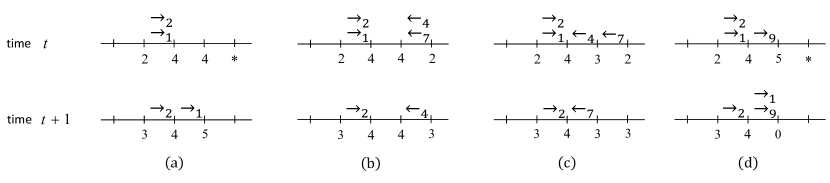
Figure 1: Queuing and annihilation rules for the particle system expansion of the $6$-color FCA on $\mathbb{Z}$. We denote particle $(i,\mathbf{r})$ by $\rightarrow_{i}$ and similarly for $\mathbf{l}$ particles. $*\in\mathbb{Z}_{6}\setminus\{2\}$.

Lastly, consider the case when there are right particles on two consecutive edges, namely, $(x,x+1)$ and $(x+1,x+2)$ and suppose site $x$ blinks at time $t$. If $dX_{t}(x+1,x+2)=1$, then the bottom $\mathbf{r}$ particle on the edge $(x,x+1)$ migrates to the top of the queue on the edge $(x+1,x+2)$ (see Figure 2.2 (d)).

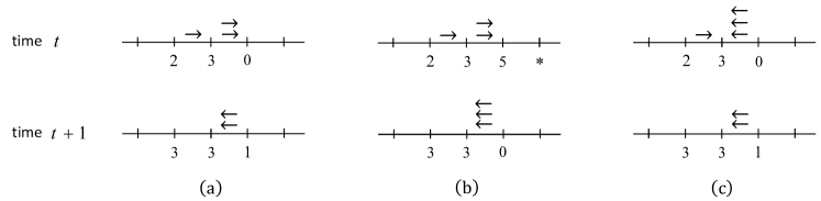
Figure 2: Particle flipping for (a) $\kappa=5$ and (b) $\kappa=6$, which are not incorporated in the particle system expansion $(\xi_{t})_{t\geq a}$. $*\in\mathbb{Z}_{6}\setminus\{2\}$. (c) By definition of $dX$, when $\kappa$ is even, edges with maximal number $\kappa/2$ of particles do not flip.

However, the particle system $\xi_{t}$ defined above misses the following phenomenon, which occurs in $dX_{t}$. If $\kappa=6$, $X_{t}(x)=2$, $dX_{t}(x,x+1)=1$, $dX_{t}(x+1,x+2)=2$ and $X_{t}(x+3)=*\neq 2$, then in the next step $dX_{t}(x+1,x+2)=-3$ (see Figure 2 (b)); in the particle system, this would correspond to the right-moving particles at $(x+1,x+2)$ “flipping” to become left-moving. A similar particle flipping scenario for $\kappa=5$ is illustrated in Figure 2 (a). Formally, we say that an edge $(x,x+1)$ (or particles on it) flips at time $t\geq 0$ if $dX_{t}(x,x+1)$ and $dX_{t+1}(x,x+1)$ have the opposite sign. It is easy to see that this happens if and only if either

$$dX_{t}(x,x+1)\geq b(\kappa) x t$$ and is excited at time

or

$$\text{$dX_{t}(x,x+1)\leq-b(\kappa)$ and $x+1$ is excited at time $t$}.$$

See Figure 2 for an illustration. In fact, we will show that particle flipping is a transient phenomenon; it occurs only during a finite “burn-in” period, after which the particles follow only the annihilation and queuing rules defining the dynamics of $\xi_{t}$. This is given by the following proposition, whose proof we delay to the end of this section:

Proposition 2.1.

Let $G=(V,E)$ be a simple connected graph with maximum degree $\leq 2$. Fix $\kappa\geq 3$, and let $(X_{t})_{t\geq 0}$ be a $\kappa$-color FCA trajectory on $G$ starting from an arbitrary deterministic coloring $X_{0}$. Then the following hold:

(i)

For $\kappa$ odd, no edge flips at any time $t\geq\lfloor\kappa/2\rfloor$;

(ii)

For $\kappa$ even, no edge flips at any time $t\geq 5\kappa$.

From now on in this section, $\kappa$ denotes an integer $\geq 3$, $(X_{t})_{t\geq 0}$ denotes a $\kappa$-color FCA trajectory on $\mathbb{Z}$ starting from an arbitrary deterministic initial coloring $X_{0}$. Proposition 2.1 guarantees the existence of an integer $0\leq t_{0}\leq 5\kappa$ after which no particle flips in the dynamics. $(\xi_{t})_{t\geq t_{0}}=(\xi_{t;t_{0}})_{t\geq t_{0}}$ denotes the particle system expansion initialized at time $t=t_{0}$. In the following lemma, we show that the particle system expansion is compatible with the original dynamics.

Lemma 2.2.

Let $(X_{t})_{t\geq 0}$, $0\leq t_{0}\leq 5\kappa$, and $(\xi_{t})_{t\geq t_{0}}$ be as before. Then for each $t\geq t_{0}$ and $x\in\mathbb{Z}$, the edge $(x,x+1)$ does not have both $\mathbf{r}$ and $\mathbf{l}$ particles at the same time and

$$dX_{t}(x,x+1)=\#\{\text{$\mathbf{r}$ particles on $(x,x+1)$ at time $t$}\}-\#\{\text{$\mathbf{l}$ particles on $(x,x+1)$ at time $t$}\}.$$ (12)

Proof.

The first part of the assertion follows from the construction of initial particle configuration $\xi_{t_{0}}$ and the annihilation rule. We show the second assertion by an induction on $t\geq t_{0}$. The base case $t=t_{0}$ is clear from the construction, so assume the assertion holds for $t\geq t_{0}$. Fix an edge $(x,x+1)$. By symmetry we may assume $dX_{t}(x,x+1)=k\geq 0$. First suppose $X_{t}(x)=b(\kappa)$. If $k=0$, then $X_{t}(x+1)=b(\kappa)$ and $X_{t+1}(x)=X_{t+1}(x+1)=b(\kappa)+1$ so $dX_{t+1}(x,x+1)=0$. On the other hand, there was no particle on the edge $(x,x+1)$ and also there is no incoming particle into the edge $(x,x+1)$ since $X_{t}(x)=X_{t}(x+1)=b(\kappa)$. Thus there is no particle on the edge $(x,x+1)$ at time $t+1$ as desired. Now suppose $k>0$. In this case $x+1$ is excited by $x$ so that $dX_{t+1}(x,x+1)=k-1\geq 0$. In the particle system, the bottom $\mathbf{r}$ particle on the edge $(x,x+1)$ is released at time $t$ and there is no incoming $\mathbf{r}$ particle from the edge $(x-1,x)$ into $(x,x+1)$. Hence whether the released $\mathbf{r}$ particle is annihilated or not, the edge $(x,x+1)$ will have $k-1$ $\mathbf{r}$ particles at time $t+1$, as desired.

Suppose $X_{t}(x)\neq b(\kappa)$ so that the edge $(x,x+1)$ is inert at time $t$. If neither $x$ nor $x+1$ are excited at time $t$, then both advance their states so that $dX_{t+1}(x,x+1)=dX_{t}(x,x+1)=k$; in parallel, there is no incoming particle into the edge $(x,x+1)$ and also no particle is released. If both $x$ and $x+1$ are excited at time $t$, then they keep the same states so that $dX_{t+1}(x,x+1)=dX_{t}(x,x+1)=k$, which is in agreement with the fact that an $\mathbf{r}$ particle coming from the edge $(x-1,x)$ moves to the top of the queue on the edge $(x,x+1)$, while the bottom $\mathbf{r}$ particle is annihilated by the $\mathbf{l}$ particle coming from the edge $(x+1,x+2)$. There are two remaining cases. Suppose only $x+1$ is excited at time $t$. Then $dX_{t+1}(x,x+1)=k-1$, and in the particle system the $\mathbf{l}$ particle coming from the edge $(x+1,x+2)$ annihilates the bottom $\mathbf{r}$ particle on the edge $(x,x+1)$, while there is no incoming $\mathbf{r}$ particle from left. Lastly, suppose only $x$ is excited at time $t$. This is the only case in which particles on the edge $(x,x+1)$ could flip, but Proposition 2.1 rules this out for $t\geq t_{0}$. Therefore, in this last case we know that $k<\left\lfloor(\kappa-1)/2\right\rfloor$, so $dX_{t+1}(x,x+1)=k+1$. In the particle system, the edge $(x,x+1)$ receives an $\mathbf{r}$ particle, which moves to the top of the queue, so there are $k+1$ $\mathbf{r}$ particles at time $t+1$. This proves the assertion. ∎

The following lemma translates the temporal event of seeing a particle on a particular edge at time $t$ into the spatial event of having positive partial sums at prior times; this is analogous to a duality relation in the graphical construction of an interacting particle system, in which one tracks the origin of a particle backwards in time. It will be crucial in Sections 3 and 5.

Lemma 2.3.

Let $(X_{t})_{t\geq 0}$, $0\leq t_{0}\leq 5\kappa$, and $(\xi_{t})_{t\geq t_{0}}$ be as before. Then we have the followings:

(i)

Every particle moves in its prescribed direction until annihilation with speed between $1/\lfloor\kappa/2\rfloor(\kappa+1)$ and $1/(b(\kappa)+2)$. If $\kappa=3$, every particle moves once in every $3$ time steps, so the speed is $1/3$.

(ii)

Suppose the particle labeled $(i,\mathbf{r})$ is on the edge $(0,1)$ at time $t=a+\tau$. Then $(i,\mathbf{r})$ was on edge $(x,x+1)$ at time $t=a$ for some $x\in[-\tau/(b(\kappa)+2),-\tau/\left\lfloor\kappa/2\right\rfloor(k+1)]$ and

$$\sum_{i=x+1}^{x+k}dX_{a}(i,i+1)\geq-\left\lfloor\kappa/2\right\rfloor+1\qquad\text{for all $1\leq k\leq\tau/\left\lfloor\kappa/2\right\rfloor(k+1)$}.$$ (13)

(iii)

Suppose $\kappa=3$. Then $(i,\mathbf{r})$ is on the edge $(0,1)$ at time $t=a+3\tau$ if and only if $(i,\mathbf{r})$ was on edge $(-\tau,-\tau+1)$ at time $t=a$ and

$$\sum_{i=-\tau+1}^{-\tau+k}dX_{a}(i,i+1)\geq 0\qquad\text{for all $1\leq k\leq 2\tau$}.$$ (14)

Proof.

To show (i), suppose $(i,\mathbf{r})$ is released from an edge $(y,y+1)$ at time $t\geq a$ and eventually released again from the edge $(y+1,y+2)$ without being annihilated. Note that $(y+1,y+2)$ must have either no particles or some $\mathbf{r}$ particles at time $t$. Suppose the former, which is always the case when $\kappa=3$. We have $X_{t}(y)=b(\kappa)$ and $X_{t}(y+1)=X_{t}(y+2)\in(b(\kappa),\kappa-1]$, so the time of the next blink of $y+1$ is between $t+b(\kappa)+2$ and $t+\kappa$. In particular, this shows the assertion for $\kappa=3$. On the other hand, since we are assuming that no particle flips after time $t=a$, there could be at most $\lfloor\kappa/2\rfloor-1$ $\mathbf{r}$ particles on the edge $(y+1,y+2)$ at time $t$. Note that $y+1$ can be excited only by $y$ until all $\mathbf{r}$ particles on $(y+1,y+2)$ have been released, so $y+1$ blinks at least once in every $\kappa+1$ seconds until then. Hence it takes at most $\lfloor\kappa/2\rfloor(\kappa+1)$ seconds for $(y+1,y+2)$ to release $(i,\mathbf{r})$. This shows (i).

The first part of (ii) follows from (i). To see the second part, observe that if $(i,\mathbf{r})$ was at height 0 (first in its queue) at time $t=a$, in order for it to reach the edge $(0,1)$, the number of $\mathbf{r}$ particles must exceed the number of $\mathbf{l}$ particles on every interval $[x,x+i]\subset[x,0]$. This observation and Lemma 2.2 imply the partial sums in (ii) are nonnegative. In general, $(i,\mathbf{r})$ could be at height at most $\left\lfloor\kappa/2\right\rfloor$, in which case $(i,\mathbf{r})$ starts with at most $\left\lfloor\kappa/2\right\rfloor-1$ $\mathbf{r}$ particles ahead of it, which defined it against $\mathbf{l}$ particles. Hence the partial sums must be bounded below by at least $-\left\lfloor\kappa/2\right\rfloor+1$.

For (iii), first suppose that $(i,\mathbf{r})$ is on the edge $(0,1)$ at time $t=a+3\tau$. By (i), $(i,\mathbf{r})$ was on the edge $(-\tau,-\tau+1)$ at time $t=a$. If for some $k\in[1,2\tau]$,

$$\sum_{i=-\tau+1}^{-\tau+k}dX_{a}(i,i+1)<0,$$ (15)

then Lemma 2.2 implies that there are more $\mathbf{l}$ particles than $\mathbf{r}$ particles in the interval $[-\tau+1,-\tau+k+1]$. One of these extra $\mathbf{l}$ particles will annihilate with $(i,\mathbf{r})$ by time $a+3\left\lceil k/2\right\rceil\leq a+3\tau$, which is a contradiction, so we must have all partial sums nonnegative. Conversely, suppose $(i,\mathbf{r})$ starts on the edge $(-\tau,-\tau+1)$ at time $t=a$ and is annihilated at time $t=a+3r+s$, where $0\leq r\leq\tau$, $0\leq s\leq 2$, and $3r+s\leq 3\tau$. Then there must be the same number of $\mathbf{l}$ particles as $\mathbf{r}$ particles in at least one of the intervals: $[-\tau,-\tau+2r]$, $[-\tau,-\tau+2r+1]$ or $[-\tau,-\tau+2r+2]$ at time $t=a$, depending on the initial position of the $\mathbf{l}$ particle that annihilates $(i,\mathbf{r})$, the timing of when the particles jump (observe that these two particles must jump at the same time, since they ultimately annihilate), and whether or not $s>0$ (if $s=0$, then the last interval can be excluded). By Lemma 2.2, this implies that the partial sum in (iii) is negative for some $k\in\{2r-1,2r,2r+1\}$ (if $s=0$, $k\in\{2r-1,2r\}$), which proves the assertion. ∎

Proof of Proposition 2.1. Suppose $\kappa=2m+1$ for some $m\in\mathbb{N}$. Note that $b(\kappa)=m$. To show (i), suppose for the sake of contradiction that an edge $(x,x+1)$ flips at time $t\geq m$. We may assume without loss of generality that $dX_{t}(x_{1},x_{2})=m$ and $x_{1}$ is excited at time $t$. This requires $X_{t}(x_{1})=m+k$ for some $k\in[1,m]$ and $x_{1}$ has another neighbor $x_{0}\in V$ such that $X_{t}(x_{0})=m$. This yields $X_{t}(x_{2})\equiv 2m+k\equiv k-1\in[0,m-1]$ modulo $\kappa=2m+1$. Since $x_{2}$ cannot be excited when its color is $<b(\kappa)=m$, it follows that $X_{t-k+1}(x_{2})=0$ and $X_{t-k}=2m$. On the other hand, note that $x_{1}$ has no neighbors besides $x_{0}$ and $x_{2}$, neither of which blinks during the time interval $[t-k,t-1]$. Hence it follows that $X_{t-k}(x_{1})=m$. But then $x_{1}$ excites $x_{2}$ at time $t-k$, so we must have $X_{t-k+1}(x_{2})=2m$, a contradiction.

Now suppose $\kappa=2m$ for some integer $m\geq 2$. We use a similar backtracking argument to rule out flipping particles after a constant time depending on $m$. Recall that $b(2m)=m-1$ is the blinking color here. Suppose, for the sake of contradiction, we have a flipping particle on edge $x_{1}x_{2}$ at time $t=N$ for some integer $N>10m$. We first claim that $\{X_{t_{1}}(x_{1}),X_{t_{1}}(x_{2})\}=\{m-1,2m-1\}$ for some $t_{1}\geq 9m$. Without loss of generality, we may assume $dX_{N}(x_{1},x_{2})=m-1$ and $x_{1}$ is excited by a blinking neighbor $x_{0}\neq x_{2}$ at time $t=N$. So $X_{N}(x_{0})=m-1$, $X_{N}(x_{1})=m-1+k$ for some $k\in[1,m]$, and $X_{N}(x_{2})\equiv 2m-2+k\equiv k-2$ modulo $\kappa=2m$. As before, none of $x_{0}$ and $x_{2}$ blink during time interval $(N-k,N]$, so backtracking $k-2$ iterations gives $X_{N-k-2}(x_{1})=m+1$ and $X_{N-k-2}(x_{2})=0$ and one more iteration gives $X_{N-k-1}(x_{1})=m$ and $X_{N-k-1}(x_{2})=2m-1$. This yields $X_{N-k}(x_{1})=m-1$ and $X_{N-k-2}(x_{2})=2m-1$ since $x_{1}$ excites $x_{2}$ at time $t_{1}:=N-k$. This shows the claim.

Next, we show that as we further backtrack the dynamics, the same “opposite” local configuration $\{X_{t}(x_{1}),X_{t}(x_{2})\}=\{m-1,2m-1\}$ appears with period $m+1$. Since $t_{1}\geq 9m\geq 6(m+1)$, this yields that the same pattern appears at least seven times during $[0,t_{1}]$. We will then obtain a contradiction. For simplicity, we work with $\kappa=6$ case but generalizing to any even $\kappa$ is immediate.

In the following backtracking tables, time increases from right to left and each column gives a local configuration on $x_{1}$, $x_{2}$ and their neighbors. The first column shows the opposite local configuration at $t=t_{1}$.

$$\begin{matrix}x_{0}&a_{1}&a_{2}&a_{3}&a_{4}\\ x_{1}&\mathbf{2}&1&0&5\\ x_{2}&5&&&*&\\ x_{3}&b_{1}&b_{2}&b_{3}&b_{4}\end{matrix}$$ (16)

While $x_{2}$ may or may not have a neighbor $x_{3}\neq x_{1}$, observe that $*=2$ in the above table contradicts the transition rule, which is the case if $x_{3}$ is absent. Hence $x_{3}$ must be present and we can extend the table as follows:

$$\begin{matrix}x_{0}&a_{1}&a_{2}&a_{3}&a_{4}&a_{5}&a_{6}&a_{7}&a_{8}\\ x_{1}&\mathbf{2}&1&0&5&5\\ x_{2}&5&&&&\textbf{2}&1&0&5\\ x_{3}&b_{1}&b_{2}&b_{3}&b_{4}&b_{5}&b_{6}&b_{7}&b_{8}\end{matrix}$$ (17)

with $2\in\{b_{2},b_{3},b_{4}\}$. But note that $b_{2}\neq 2$ since otherwise we have $b_{4}=0$ and $b_{5}=5$, which contradict the transition rule since then $x_{2}$ would excite $x_{3}$ at the column containing $b_{5}$ so that $b_{4}=5$. Notice that the column containing $a_{5}$ is identical to the first one with the role of $x_{1}$ and $x_{2}$ exchanged. Hence the opposite local configuration appears with period $4=m+1$.

Since $t_{1}\geq 6(m+1)$, we further extend our backtracking table as follow:

$$\setcounter{MaxMatrixCols}{14}\begin{matrix}x_{0}&a_{1}&a_{2}&a_{3}&a_{4}&a_{5}&a_{6}&a_{7}&a_{8}&a_{9}&a_{10}&a_{11}&a_{12}&a_{13}\\ x_{1}&\mathbf{2}&1&0&5&5&&&&\textbf{2}&1&0&5&5\\ x_{2}&5&&&&\textbf{2}&1&0&5&5&&&&\mathbf{2}\\ x_{3}&b_{1}&b_{2}&\mathbf{b_{3}}&\mathbf{b_{4}}&b_{5}&b_{6}&b_{7}&b_{8}&b_{9}&b_{10}&\mathbf{b_{11}}&\mathbf{b_{12}}&b_{13}\\ \end{matrix}$$ (18)

where $2\in\{b_{3},b_{4}\}$ and $2\in\{b_{11},b_{12}\}$ by repeating the same argument. In fact, none of the four combinations is possible. Suppose $b_{3}=2$. Then $b_{5}=0$, so $x_{2}$ does not excite $x_{3}$ at the column containing $b_{5}$. But then by the degree condition, $x_{3}$ must have been excited by at most once during the transition $b_{3}\leftarrow b_{11}$, which is impossible as this transition requires two excitations. Thus $b_{4}=2$. Since we we have enough history to apply the same argument to $b_{11}$ and $b_{12}$, we conclude $b_{12}=2$. But then by a similar argument the transition $2=b_{4}\leftarrow b_{12}=2$ is impossible. This shows the assertion. $\blacksquare$

3 Proof of Theorem 2 (i): Upper bound on the probability of local disagreement at time $t$

In this section we prove Theorem 2 (i). Fix an integer $\kappa\geq 3$. We define our probability space $(\Omega,\mathcal{F},\mathbb{P})$ as follows. Let $\Omega=\mathbb{Z}_{\kappa}^{\mathbb{Z}}$, let $\mathcal{F}$ be the $\sigma$-algebra generated by finite cylinder sets of $\Omega$, and let $\mathbb{P}$ be the uniform product measure on $\Omega$. Let $X_{0}$ be a random $\kappa$ coloring on $\mathbb{Z}$ drawn from $\mathbb{P}$, that is, $\mathbb{P}(\pi_{n}\circ X_{0}=i)=1/\kappa$ for all $n\in\mathbb{Z}$ and $i\in\mathbb{Z}_{\kappa}$, where $\pi_{n}$ is the projection onto the site $n\in\mathbb{Z}$. By iterating the $\kappa$-color FCA transition map on each sample coloring of $X_{0}$, one obtains a process $(X_{t})_{t\geq 0}$. This induces an associated process $(dX_{t})_{t\geq 0}$, referring to the definition given in (11).

In order to show the first part of Theorem 2, by symmetry under the transformation $X_{t}\mapsto-X_{t}$, it suffices to show that

$$\mathbb{P}(dX_{t}(x,x+1)>0)=O(t^{-1/2}).$$ (19)

By the particle system expansion and Lemma 2.2, $dX_{5\kappa+\tau}(x,x+1)>0$ implies that there exists a unique $\mathbf{r}$ particle at time $t=t_{0}$, say $(\mathbf{r},i)$, which is not annihilated by an $\mathbf{l}$ particle through time $t=5\kappa+\tau$ and reaches the bottom of the queue at edge $(x,x+1)$ at time $t=5\kappa+\tau$. This event is contained in the event that the particle $(\mathbf{r},i)$ survives upto time $t=5\kappa+\tau$. By translation invariance of the initial product measure and the FCA dynamics, therefore it suffices to show that a $\mathbf{r}$ particle on the edge $(0,1)$ at time $5\kappa$ survives upto time $t=5\kappa+\tau$ with probability at most $O(t^{-1/2})$. We define the associated random walk $\{S_{n}\}_{n\geq 0}$ by $S_{0}=0$ and $S_{n}=\sum_{i=0}^{n-1}dX_{5\kappa}(i,i+1)$. Then by Proposition 2.3, it suffices to show the following statement:

$$\mathbb{P}\left(S_{1}\geq b,\cdots,S_{t}\geq b\right)=O(t^{-1/2})\quad\forall b\geq 0.$$ (20)

The probability on the left hand side of the above equation is called a survival probability of a random walk and is of particular interest in many situations that arises in non-equilibrium systems (see [3] for a recent survey on this topic). The survival probability of a simple random walk was first obtained explicitly by Sparre Anderson [1], which has been generalized by Feller [6] to arbitrary random walks with i.i.d. increments satisfying some moment conditions (see Theorem 3.3.). However, our random walk $S_{n}$ has correlated increments $dX_{5\kappa}(n,n+1)$, so known result for i.i.d. increments does not directly apply.

To overcome this difficulty, we construct a coarse-grained random walk from our original locally dependent random walk so that the “chunked” increments become independent. We proceed as follows. Fix an integer $c\geq 1$, and let $B_{0}\geq 0$ be a (random) integer given by

$$B_{0}=\inf\{b\geq 0\,:\,\text{$X_{0}\equiv 0$ on $[b-c+1,b+c]$ and $0\notin\{X_{0}(b-c),X_{0}(b+c+1)\}$}\}$$ (21)

Having defined $B_{i}$ and $B_{-i}$ for $i\geq 0$, we define $B_{i+1}$ and $B_{-i-1}$ recursively as

$$B_{i+1}=\inf\{b\geq B_{i}\,:\,\text{$X_{0}\equiv 0$ on $[b-c+1,b+c]$ and $0\notin\{X_{0}(b-c),X_{0}(b+c+1)\}$}\},$$ (22)

$$B_{-i-1}=\sup\{b\leq B_{-i}\,:\,\text{$X_{0}\equiv 0$ on $[b-c+1,b+c]$ and $0\notin\{X_{0}(b-c),X_{0}(b+c+1)\}$}\}.$$ (23)

Since $X_{0}$ is drawn from the uniform product measure, this random sequence $(B_{i})_{i\in\mathbb{Z}}$ is well-defined with probability 1. For each $i\in\mathbb{Z}$, denote $A_{i}=B_{i-1}+c$. Then by the construction, the initial coloring $X_{0}$ is identically zero on each interval $[B_{i}-c+1,A_{i+1}+c-1]$ and nonzero at sites $B_{i}-c$ and $A_{i+1}+c$. Hence these intervals are all disjoint, and induces a random partition $(I_{i})_{i\in\mathbb{Z}}$ of $\mathbb{Z}$ where $I_{i}=[A_{i},B_{i}]$ (see Figure 3).

The idea is that if $c>0$ is large enough, then these consecutive zeros act as buffer regions so that there is no interaction between sites in different intervals during the burn-in period. Since each site blinks at most once in every $\kappa$ seconds and each site affects its neighboring site only when it blinks, the speed of information propagation is at most $1/\kappa$. Since the burn-in period is at most $5\kappa$ seconds, we may take $c=6$. Let $\zeta_{i}:=\sum_{j\in I_{i}}dX_{5\kappa}(j,j+1)$ for each $i\in\mathbb{Z}$, and define the chunked associated random walk $(\overline{S}_{n})_{n\geq 0}$ by $\overline{S}_{0}=0$ and $\overline{S}_{n}=\sum_{i=1}^{n}\zeta_{i}$.

Figure 3: Initial random coloring $X_{0}$ induces a partition of $\mathbb{Z}$ into random intervals with exactly $6$ consecutive sites on the left and right having initial color 0. $*$’s indicates nonzero colors and $?$’s are arbitrary. At time $t=5\kappa$, there is at least one 0 on left and right of each interval.

We first verify that the chunked increments $\zeta_{i}$’s are i.i.d. with finite moments.

Proposition 3.3.

$\zeta_{i}$’s are i.i.d. with mean zero and finite variance.

Proof.

That $\zeta_{i}$’s are identically distributed is clear from the construction, and that they have mean zero follows from symmetry. Note that each random interval $I_{i}$ has geometrically distributed length. Since $dX_{5\kappa}$ is uniformly bounded, it follows that each $\zeta_{i}$ has finite variance.

It remains to show the independence. To this end, we trace information propagation back in time from $t=5\kappa$ to $t=0$. Namely, for each $x\in\mathbb{Z}$, we are going to define an ascending sets of integers $N^{(0)}(x)\subseteq N^{(1)}(x)\subseteq\cdots\subseteq N^{(5\kappa)}(x)$ recursively as follows: $N^{(0)}(x)=\{x\}$ and

$$N^{(i+1)}(x)=N^{(i)}(x)\cup\{y\in\mathbb{Z}\,:\,\text{$y$ excites any site in $N^{(i)}(x)$ at time $t=5\kappa-i-1$}\}.$$ (24)

In words, $N^{(5\kappa)}(x)$ contains all sites whose initial color could affect $X_{5\kappa}(x)$. Note that $X_{5\kappa}(x)$ is completely determined by the initial colors of sites in $N^{(5\kappa)}(x)$. Moreover, since $dX_{5\kappa}(B_{i},A_{i+1})=0$ for all $i\in\mathbb{Z}$, $\zeta_{i}$ depends only on the initial colors in $I_{i}$. Hence it is enough to show that for any $i\in\mathbb{Z}$ and $x\in I_{i}$, we have $N^{(5\kappa)}(x)\subseteq I_{i}$.

Let $I_{i}=[A_{i},B_{i}]$’s be the random intervals as before. Fix $i\in\mathbb{Z}$. By construction, the six sites in $[A_{i},A_{i}+6]$ have initial color 0 so they all have color $b(\kappa)$ at time $t=b(\kappa)$. So $X_{\kappa}(x)=0$ for all $x\in[A_{i},A_{i}+5]$ and none of the $x$’s gets excited during time interval $[0,\kappa]$. Repeating the same argument, we see that the site $A_{i}$ is not excited during the time interval $[0,5\kappa]$. By symmetry and translation invariance, the same observation holds for $B_{i}=A_{i}-1$ and for all $i\in\mathbb{Z}$.

Now fix $i\in\mathbb{Z}$ and $x\in I_{i}$. Suppose for contrary that $I_{i-1}\cap N^{(5\kappa)}(x)\neq\emptyset$ and let $x^{\prime}$ be in the intersection. Since every site can only excite its neighbors at any given time and since $x^{\prime}\leq B_{i-1}<A_{i}\leq x$, this implies that $A_{i}$ is excited by $B_{i-1}$ at some time during $[0,5\kappa]$, which contradicts the observation in the previous paragraph. Hence $I_{i-1}\cap N^{(5\kappa)}(x)=\emptyset$. Similarly $N^{(5\kappa)}(x)\cap I_{i+1}=\emptyset$. This shows $N^{(5\kappa)}(x)\subseteq I_{i}$ as desired. ∎

Next, we recap some results on survival probabilities of random walks with i.i.d. increments. For its statement, let $\mathtt{X}_{1},\mathtt{X}_{2}\cdots,$ be i.i.d. integer valued random variables such that $\mathbb{E}[\mathtt{X}_{1}]=0$ and $\mathbb{E}[\mathtt{X}_{1}^{2}]\in(0,\infty)$. Define a random walk $(S_{n})_{n\geq 0}$ by $\mathtt{S}_{n}=\mathtt{S}_{n-1}+\mathtt{X}_{n}$ for $n\geq 1$ and $\mathtt{S}_{0}=x$ is to be specified. Define survival probabilities

$$\mathtt{Q}(x,t)=\mathbb{P}(\mathtt{S}_{1}\geq 0,\mathtt{S}_{2}\geq 0,\cdots,\mathtt{S}_{t}\geq 0\,|\,\mathtt{S}_{0}=x)\quad\text{$\forall x,t\geq 0$}.$$ (25)

Note that $\mathtt{Q}(x,t)\geq\mathtt{Q}(x,t+1)$ for all $x,t\geq 0$. We are interested in the asymptotic behavior of the sequences $(\mathtt{Q}(x,t))_{t\geq 0}$ for each $x\geq 0$. This is closely related to the asymptotic behavior of their generating functions

$$\widetilde{\mathtt{Q}}_{x}(u):=\sum_{t\geq 0}u^{t}Q(x,t)$$ (26)

as $u\nearrow 1$ by a Tauberian theorem (see e.g., Theorem 5 of Chapter XIII in [6]).

Lemma 3.2.

For each $x\geq 0$ and $u\in[0,1)$, we have

$$\widetilde{\mathtt{Q}}_{x}(u)\leq(x+1)\widetilde{\mathtt{Q}}_{0}(u).$$ (27)

Proof.

Let

$$M=M(x,t):=\min_{0\leq k\leq t}\{\mathtt{S}_{k}\,|\,\mathtt{S}_{0}=x\}$$ (28)

and

$$\tau=\tau(x,t):=\min\{0\leq k\leq t\,:\,\mathtt{S}_{k}=M(x,t)\}.$$ (29)

For each $0\leq i\leq x$ and $0\leq j\leq t$, denote

$$a(i,j)=\mathbb{P}\left(\mathtt{S}_{0}\geq i,\mathtt{S}_{1}\geq i,\,\cdots,\mathtt{S}_{j-1}\geq i,\,\mathtt{S}_{j}=i\,|\,\mathtt{S}_{0}=x\right).$$ (30)

Note that for each $0\leq i\leq x$ and $u\in[0,1)$, we have

$$\sum_{j=0}^{\infty}a(i,j)u^{j}\leq\sum_{j=0}^{\infty}a(i,j)=\mathbb{P}\left[\text{$M(x,t)=i$ for some $t\geq 0$}\right]\leq 1.$$ (31)

Now by Markov property of $\mathtt{S}_{n}$,

$$\mathtt{Q}(x,t)=\mathbb{P}(M(x,t)\geq 0)=\sum_{i=0}^{x}\sum_{j=0}^{t}a(i,j)\mathtt{Q}(0,t-j).$$ (32)

Multiplying by $u^{t}$ and summing over all $t\geq 0$, we obtain

$$\widetilde{\mathtt{Q}}_{x}(u) = \sum_{i=0}^{x}\sum_{t=0}^{\infty}\sum_{j=0}^{t}a(i,j)u^{t}\mathtt{Q}(0,t-j)$$ (33)

$$= \sum_{i=0}^{x}\sum_{j=0}^{\infty}a(i,j)u^{j}\sum_{t=j}^{\infty}u^{t-j}\mathtt{Q}(0,t-j)$$ (34)

$$= \left(\sum_{i=0}^{x}\sum_{j=0}^{\infty}a(i,j)u^{j}\right)\widetilde{\mathtt{Q}}_{0}(u)$$ (35)

where for we have used Fubini’s theorem for the second equality. Then the assertion follows from (31). ∎

For two functions $f$ and $g$, we say $f\sim g$ if $\lim_{t\rightarrow\infty}f(t)/g(t)=1$. The following theorem gives the asymptotic behavior of $\mathtt{Q}(0,t)$ as $t\rightarrow\infty$, and hence that of $\widetilde{\mathtt{Q}}_{0}(u)$ as $u\nearrow 1$:

Theorem 3.3. ( Feller [6]).

There exists $c\in(-\infty,\infty)$ such that

$$\sum_{n=1}^{\infty}\frac{1}{n}\left(\mathbb{P}(\mathtt{S}_{n}>0)-\frac{1}{2}\right)=c.$$

Furthermore, we have

$$\mathtt{Q}(0,t)\sim\frac{e^{-c}}{\sqrt{\pi}}\frac{1}{\sqrt{t}}.$$ (36)

We are now ready to give a proof of the first part of Theorem 2.

Proof of Theorem 2 (i). Let $(I_{i})_{i\in\mathbb{Z}}=([A_{i},B_{i}])_{i\in\mathbb{Z}}$ be the random partition of $\mathbb{Z}$ as before. We may assume without loss of generality that $I_{0}$ contains the origin. Fix arbitrary $b\geq 0$, and let $D$ be the first crossing time of level $-b$ of the associated walk, i.e.,

$$D=\inf\{n\geq 0\,:\,S_{1}>-b,S_{2}>-b,\cdots,S_{n-1}>-b,S_{n}\leq-b\}.$$ (37)

By the discussion in the beginning of Section 3, it suffices to show (20), which is equivalent to

$$\mathbb{P}(D\geq n)=O(n^{-1/2}).$$ (38)

Let $N(t)$ be the maximal integer such that $I_{0}\cup I_{1}\cup\cdots\cup I_{N(t)}\subset[A_{0},t)$. Let $\mu:=\mathbb{E}(|I_{1}|)\in[1,\infty)$. Then we have

$$t\leq|I_{0}|+\cdots+|I_{N(t)}|+|I_{N(t)+1}|.$$ (39)

By partitioning on the value of $N(D)$,

$$\mathbb{P}(D\geq n) \leq \mathbb{P}(D\geq n,N(D)\geq n/2\mu)+\mathbb{P}(D\geq n,N(D)<n/2\mu)$$

$$\leq \mathbb{P}\left(S_{B_{1}}\geq-b,\,S_{B_{1}}+\overline{S}_{1}\geq-b,\,\cdots,S_{B_{1}}+\overline{S}_{\lfloor n/2\mu\rfloor}\geq-b\right)+\mathbb{P}\left(|I_{0}|+\cdots+|I_{\lceil n/2\mu\rceil}|\geq 2\cdot n/2\right).$$

Since $|I_{i}|$’s are i.i.d. with exponential tail, the second term in the last expression is exponentially small by a large deviation principle (see, e.g., Dembo [4]). If we denote the event in the first probability by $\Omega_{n}$, then it suffices to show that

$$\mathbb{P}(\Omega_{n})=O(n^{-1/2}).$$ (40)

To this end, define its generating function

$$F(u)=\sum_{n=0}^{\infty}\mathbb{P}(\Omega_{n})u^{n}.$$ (41)

By Tauberian theorem (see e.g., Theorem 5 of Chapter XIII in [6]) and Theorem 3.3., it suffices to show that

$$F(u)\leq C\widetilde{Q}_{0}(u)$$ (42)

for some constant $C>0$. We first partition $\Omega_{n}$ according to the values of $S_{B_{1}}$. Note that the probability $\mathbb{P}(S_{B_{1}}=s)$ is exponentially small in $s$, since $S_{B_{1}}\leq\kappa|I_{0}|$ and $|I_{0}|$ has exponential tail. Hence we have

$$\mathbb{P}(\Omega_{n}) = \sum_{s=-b}^{\infty}\mathbb{P}(S_{B_{1}}=s)\,\mathbb{P}\left(\overline{S}_{1}\geq-b-s,\,\cdots,\overline{S}_{\lfloor n/2\mu\rfloor}\geq-b-s\right)$$ (43)

$$\leq \sum_{s=-b}^{\infty}e^{-cs}Q(b+s,\lfloor n/2\mu\rfloor).$$ (44)

for some constant $c>0$. Multiplying by $u^{n}$ and summing over all $n\geq 0$, together with the fact that $u\in[0,1)$ and Lemma 3.2, we obtain

$$F(u) \leq \sum_{s=-b}^{\infty}e^{-cs}\sum_{n=0}^{\infty}u^{n}Q(b+s,\lfloor n/2\mu\rfloor)$$ (45)

$$\leq \sum_{s=-b}^{\infty}e^{-cs}\sum_{n=0}^{\infty}u^{\lfloor n/2\mu\rfloor}Q(b+s,\lfloor n/2\mu\rfloor)$$ (46)

$$\leq \sum_{s=-b}^{\infty}e^{-cs}\sum_{t=0}^{\infty}(2\mu+1)u^{t}Q(b+s,t)$$ (47)

$$= (2\mu+1)\sum_{s=-b}^{\infty}e^{-cs}\widetilde{Q}_{b+s}(u)$$ (48)

$$\leq (2\mu+1)\widetilde{Q}_{0}(u)\left(\sum_{s=-b}^{\infty}e^{-cs}(b+s+1)\right)$$ (49)

This shows (42) as desired, and completes the proof of the assertion. $\blacksquare$

4 Tournament expansion of the FCA dynamics on $\mathbb{Z}$

Particle system expansion of the FCA dynamics has been successful in getting an upper bound on the probability $\mathbb{P}(X_{t}(x)\neq X_{t}(x+1))$ of local disagreement at time $t$. We handled the local dependence on the edge particles developed during the burn-in period by coarse-graining our associated locally correlated random walk into a “chunked” random walk by giving up bounded increments but retrieving independent increments in return. However, this technique does not readily produce the matching lower bound; see Section 6, wherein we obtain precise asymptotics for $\kappa=3$. In this section, we introduce another comparison process for FCA with a slightly different perspective, which we call the tournament expansion. We originally developed the tournament expansion with Gravner in [10] in order to better understand the CCA and GHM dynamics, and a corresponding expansion of the FCA dynamics has some extra details.

We begin with an instructive toy model called a tournament process. Instead of coloring nodes of a graph $G=(V,E)$ by using mod $\kappa$ colors, consider a map $\mathtt{Rk}_{0}:V\rightarrow\mathbb{Z}$ called a ranking on $G$. The transition map from time $t$ to $t+1$ is given by

$$\mathtt{Rk}_{t+1}(x)=\max\{\mathtt{Rk}_{t}(y)\,|\,y\in N(x)\cup\{x\}\}.$$ (50)

In words, in each transition $\mathtt{Rk}_{t}\mapsto\mathtt{Rk}_{t+1}$, each node simultaneously copies the maximum rank among it and its neighbors. Observe that if $G$ is finite, then for any initial ranking $\text{Rk}_{0}$ on $G$ there is a global maximum, and each node will eventually adopt the global maximum. In general, locally maximum rank propagates with unit speed across the graph until it is overcome by a higher ranker.

The basic idea of relating a similar process to the FCA dynamics on $\mathbb{Z}$ is the following: we construct an accompanying tournament-like system where each site increases its rank if and only if it gets excited. To give a detailed construction, we first define a path integral of the 1-form $dX_{t}$. A directed walk $\vec{W}$ from a site $x$ to another site $y$ in $\mathbb{Z}$ is a sequence $(x_{i})_{i=0}^{l}$ of adjacent sites in $\mathbb{Z}$ such that $x_{0}=x$ and $x_{l}=y$. Given a $\kappa$-color FCA dynamic $(X_{t})_{t\geq 0}$ on $\mathbb{Z}$, the path integral of $dX_{t}$ over a directed walk $\vec{W}=(x_{i})_{i=0}^{l}$ from $x$ to $y$ is defined by

$$\int_{x}^{y}dX_{t}:=\sum_{i=1}^{l-1}dX_{t}(x_{i},x_{i+1}).$$ (51)

Note that since $\mathbb{Z}$ is simply connected and $dX_{t}$ is anti-symmetric, any contour integral of $dX_{t}$ is zero. Hence the path integral does not depend on the choice of a directed walk between the endpoints.

Now let $(X_{t})_{t\geq 0}$ be a $\kappa$-color FCA trajectory. We define its tournament expansion by a sequence of rankings $(\mathtt{rk}_{t})_{t\geq t_{0}}$ defined as follows: set the rank of the origin at time $t$ by

$$\mathtt{rk}_{t}(0)=\mathtt{ne}_{t}(0)=\sum_{s=0}^{t-1}\mathbbm{1}(\text{0 is excited at time $s$})$$ (52)

for all $t\geq 0$, and then extend to all sites by a path integral of $-dX_{t}$:

$$\mathtt{rk}_{t}(x)-\mathtt{rk}_{t}(0)=-\int_{0}^{x}dX_{t}$$ (53)

The minus sign in front of the path integral reflects the fact that in the (inhibitory) FCA dynamics, nodes tend to adjust their phases toward those lagging the most so we are giving higher ranks to the lagging nodes. For instance, if $\kappa=6$ and $X_{t}(x)=3$ and $X_{t}(x+1)=b(6)=2$, then $x+1$ excites $x$ at time $t$ so we give $x+1$ a higher rank than $x$ at time $t$, so it is natural to require the following local relation

$$\mathtt{rk}_{t}(x+1)-\mathtt{rk}_{t}(x)=-dX_{t}(x,x+1)>0,$$ (54)

which is incorporated in our construction.

Our first observation about tournament expansion is that all sites indeed increase their rank by 1 if and only if they get excited:

Proposition 4.1.

Let $(X_{t})_{t\geq 0}$ and $(\mathtt{rk}_{t})_{t\geq 0}$ be as before, and suppose no particle flips after time $t=t_{0}\geq 0$. For any $x,y\in\mathbb{Z}$ and $t\geq t_{0}$, we have

$$\int_{x}^{y}\,dX_{t+1}-\int_{x}^{y}\,dX_{t}=\mathbbm{1}(\text{$x$ is excited at time $t$})-\mathbbm{1}(\text{$y$ is excited at time $t$}).$$ (55)

Furthermore, we have

$$\mathtt{rk}_{t+1}(x)-\mathtt{rk}_{t}(x)=\mathbbm{1}(\text{$x$ is excited at time $t$}).$$ (56)

Proof.

The second part of the assertion follows immediately from the first part, definition of rank of the origin, and the following identity

$$\mathtt{rk}_{t+1}(x)-\mathtt{rk}_{t}(x)=[\mathtt{rk}_{t+1}(0)-\mathtt{rk}_{t}(0)]-\left[\int_{0}^{x}dX_{t+1}-\int_{0}^{x}dX_{t}\right].$$ (57)

Now we show the first part. We may assume $x<y$ since both hand sides in (55) are anti-symmetric under exchanging $x$ and $y$. Observe that it suffices to show the assertion for $y=x+1$, since then

$$\sum_{i=x}^{y-1}(dX_{t+1}-dX_{t})(i,i+1) = \sum_{i=0}^{k-1}{\mathbbm{1}}(\text{$x_{i}$ is excited at time $t$})-{\mathbbm{1}}(\text{$x_{i+1}$ is excited at time $t$})$$ (58)

$$= {\mathbbm{1}}(\text{$x$ is excited at time $t$})-{\mathbbm{1}}(\text{$y$ is excited at time $t$}),$$ (59)

where the left hand side equals that of (55). It remains to verify that for any $x\in\mathbb{Z}$,

$$(dX_{t+1}-dX_{t})(x,x+1)={\mathbbm{1}}(\text{$x$ is excited at time $t$})-{\mathbbm{1}}(\text{$x+1$ is excited at time $t$})$$ (60)

for any $x\in\mathbb{Z}$. The argument is based on the particle system expansion and Lemma 2.2; namely, the left hand side of (60) equals the “flux” of particles, which we define it to be the net change in the number of $\mathbf{r}$ particles minus $\mathbf{l}$ particles on edge $(x,x+1)$ from time $t$ to $t+1$.

First assume that $x$ excites $x+1$ at time $t$, so $x$ blinks at time $t$ and is not excited at the same time, so the right hand side of (60) equals $-1$. The assumption yields that edge $(x,x+1)$ has only $\mathbf{r}$ particles, and its bottom $\mathbf{r}$ particle is released at time $t$; since $x$ is not excited at time $t$, there is no $\mathbf{r}$ particle released from $(x-1,x)$, so $(x,x+1)$ loses one $\mathbf{r}$ particle during the transition $X_{t}\mapsto X_{t+1}$. Then by Lemma 2.2, the left hand side of (60) also equals $-1$, as desired. Second, suppose that $x$ does not excite $x+1$, but $x+1$ is excited by $x+2$ at time $t$. If $x$ is also excited by $x-1$ at time $t$, then no particle leaves the edge $(x,x+1)$, but there is both an incoming $\mathbf{l}$ particle from the right and an $\mathbf{r}$ particle from the left, which annihilate each other. Thus the flux is zero as asserted. Lastly, suppose that $x+1$ is excited by $x+2$ but $x$ is not excited by $x-1$. Then $x$ is not excited at time $t$, so the right hand side of (60) equals $-1$. Indeed, no $\mathbf{r}$ particle is released from $(x-1,x)$ and a $\mathbf{l}$ particle is released from $(x+1,x+2)$ at time $t$, so either this incoming $\mathbf{l}$ particle annihilates the bottom $\mathbf{r}$ particle on $(x,x+1)$ if any, or occupies the empty queue at $(x,x+1)$; in both cases, the flux on $(x,x+1)$ is $-1$. This shows the assertion. ∎

The previous observation immediately yields that the tournament expansion for FCA dynamics does follow a tournament-like time evolution where local maxima affect their neighbors only when they blink:

Proposition 4.2.

Let $(X_{t})_{t\geq 0}$ and $(\mathtt{rk}_{t})_{t\geq 0}$ be as before, and suppose no particle flips after time $t=t_{0}\geq 0$. Then for any $t\geq t_{0}$ and $x\in\mathbb{Z}$, we have

$$\mathtt{rk}_{t+1}(x)=\begin{cases}\mathtt{rk}_{t}(x)+1&\text{if $\exists y\in N(x)$ s.t. $X_{t}(y)=b(\kappa)$ and $\mathtt{rk}_{t}(y)>\mathtt{rk}_{t}(x)$}\\ \mathtt{rk}_{t}(x)&\text{otherwise}\end{cases}$$ (61)

Proof.

Recall that $x$ is excited at time $t$ iff there exists a blinking neighbor $y\in N(x)$ with $dX_{t}(y,x)>0$, and by construction $\mathtt{rk}_{t}(y)=\mathtt{rk}_{t}(x)+dX_{t}(y,x)$. Hence the assertion follows from Proposition 4.1. ∎

Now we are ready to prove the key lemma in this section. Recall that the quantity $\mathtt{rk}_{t}(0)=\mathtt{ne}_{t}(0)$ is a “temporal” quantity in the sense that it depends on the history of trajectory $(X_{t})_{t\geq 0}$ upto time $t-1$. Define a “spatial” quantity $M_{t}(r)$ by the maximum rank at time $t$ in the $r$-ball centered at the origin, i.e.,

$$M_{t}(r)=\max\{\mathtt{rk}_{t}(x)\,:\,|x|\leq r\}.$$ (62)

The next observation relates these two quantities.

Lemma 4.3.

Let $(X_{t})_{t\geq 0}$ and $(\mathtt{rk}_{t})_{t\geq 0}$ be as before, and suppose no particle flips after time $t=t_{0}\geq 0$. Then for each $t\geq 0$, we have

$$M_{t_{0}}(t/\lfloor\kappa/2\rfloor(\kappa+1))\leq\mathtt{ne}_{t+t_{0}}(0)\leq M_{t_{0}}(t/\kappa).$$ (63)

Moreover, if $\kappa=3$, we have

$$M_{t_{0}}(t-1)\leq\mathtt{ne}_{3t+t_{0}}(0)\leq M_{t_{0}}(t).$$ (64)

Proof.

Recall that $\mathtt{ne}_{t}(0)=\mathtt{rk}_{t}(0)$ for all $t\geq 0$ by construction. By Proposition 4.2, each site increases its rank only when in contact with blinking neighbors with higher rank. This happens if and only if a particle passes through each site. By Lemma 2.3 (i), this happens at most once in every $\kappa$ seconds. In other words, the speed of information propagation is upper bounded by $1/\kappa$; by time $t+t_{0}$, the origin can adopt the highest rank within radius at most $t/\kappa$, which is $M_{t_{0}}(t/\kappa)$. This gives the second inequalities in (63) and (64).

To show the first inequality in (63), we first claim that for any $t\geq 0$, $x\in\mathbb{Z}$, we have

$$\mathtt{rk}_{t+\lfloor\kappa/2\rfloor(\kappa+1)}(x)\geq\max\{\mathtt{rk}_{t}(y)\,|\,y=x\pm 1\}.$$ (65)

In words, the rank of a site $x$ exceeds the maximum rank in its 1-ball $\lfloor\kappa/2\rfloor(\kappa+1)$ seconds ago. This gives a lower bound on the growth rate of ranks at all sites, and repeating this inequality for the origin and making a change of variable in time, the first inequality in (63) follows.

It remains to verify the claim. We may assume without loss of generality that $y=x-1$. If $\mathtt{rk}_{t}(x)\geq\mathtt{rk}_{t}(x-1)$, then by the monotonicity of ranks in time we have

$$\mathtt{rk}_{t+\lfloor\kappa/2\rfloor(\kappa+1)}(x)\geq\mathtt{rk}_{t}(x-1)$$ (66)

So we may assume $\mathtt{rk}_{t}(x)<\mathtt{rk}_{t}(x-1)$. By construction of the ranking $\mathtt{rk}_{t}$, the rank difference between adjacent sites is upper bounded by $\lVert dX_{t}\rVert_{\infty}\leq\lfloor\kappa/2\rfloor$, so we have

$$\mathtt{rk}_{t}(x)<\mathtt{rk}_{t}(x-1)\leq\mathtt{rk}_{t}(x)+\lfloor\kappa/2\rfloor.$$ (67)

On the other hand, by the monotonicty, $\mathtt{rk}_{s}(x-1)\geq\mathtt{rk}_{t}(x-1)$ for all times $s\in[t,t+\lfloor\kappa/2\rfloor(\kappa+1)]$. Hence during this time interval whenever $x-1$ blinks, $x$ increases its rank by 1 at least until $x$ has rank at least $\mathtt{rk}_{t}(x-1)$. Now it suffices to observe that $x-1$ blinks at least once in every $\kappa+1$ seconds during this period. This follows from the fact that $x-1$ is not excited by $x$ during this interval, and $x-2$ blinks at most once in every $\kappa$ seconds; hence it may take at most $\kappa+1$ seconds between consecutive blinks of $x-1$. This shows the claim. The first inequality in (64) follows from a similar argument and the fact that there could be at most one particle in each edge at each time. ∎

5 Proof of Theorem 3: Lower bound on the average rate of local disagreement

In this section we prove Theorem 3, which is complementary to Theorem 2. Let $(X_{t})_{t\geq 0}$ be a random $\kappa$-color FCA trajectory, $t_{0}\in[0,5\kappa]$ an integer such that no edges flip at all times $t\geq t_{0}$, and $(\mathtt{rk}_{t})_{t\geq 0}$ its tournament expansion. In Section 3, we have seen that the probability $\mathbb{P}(X_{t}(x)\neq X_{t}(x+1))$ of local disagreement at time $t$ was related to the survival probability of the associated random walk $S_{n}=\sum_{i=0}^{n-1}dX_{t_{0}}(i,i+1)$. The tournament expansion, especially Lemma 4.3, tells us that the total number of excitation of site $x$ upto time $t$ is related to the maximum of the associated random walk.

To handle the dependence between increments, realize the increments are a functional of an underlying Markov chain. Namely, note that the initial environment $X_{0}$ gives a Markov chain $(X_{0}(x))_{x\in\mathbb{Z}}$ of colors on sites at time $0$. Fix an integer $d\geq t_{0}/(b(\kappa)+2)$, and let $P$ be the finite path from $-d$ to $d+1$ on vertex set $V=[-d,d+1]$ with nearest neighbors, i.e., $i\sim j$ iff $|i-j|=1$. For each $x\in\mathbb{Z}$, define $\vec{X}_{0}(x)\in(\mathbb{Z}/\kappa\mathbb{Z})^{V}$ by

$$[\vec{X}_{0}(x)](i)=X_{0}(x+i)$$ (68)

for all $i\in V$. This defines a Markov chain $(\vec{X}_{0}(x))_{x\in\mathbb{Z}}$ of $2d+2$-tuples of initial colors. Let $\tau:\mathbb{Z}_{\kappa}^{V}\rightarrow\mathbb{Z}_{\kappa}^{V}$ be the $\kappa$-color FCA transition map on $P$. Define a functional $g:(\mathbb{Z}/\kappa\mathbb{Z})^{2d+2}\rightarrow[-\kappa,\kappa]$ by

$$g(\vec{X})=d\tau^{t_{0}}[\vec{X}](0,1).$$ (69)

Note that since the speed of information propagation is upper bounded by $1/(b(\kappa)+2)$ by Lemma 4.3, $(X_{t_{0}}(x),X_{t_{0}}(x+1))$ is completely determined by $\vec{X}_{0}(x)$. That is, if we denote $Y:=\tau^{t_{0}}[\vec{X}_{0}(x)]\in(\mathbb{Z}/\kappa\mathbb{Z})^{V}$, then we have

$$(Y(0),Y(1))=(X_{t_{0}}(x),X_{t_{0}}(x+1)).$$ (70)

Hence we have

$$g(\vec{X}_{0}(x))=dX_{t_{0}}(x,x+1),$$ (71)

which holds for all $x\in\mathbb{Z}$. In particular, $g(\vec{X}_{0}(x))$’s are identically distributed with mean zero and finite variance.

Now we give a proof to Theorem 3.

Proof of Theorem 3. Fix $\kappa\geq 3$, and let $(X_{t})_{t\geq 0}$, $t_{0}\in[0,5\kappa]$, $d\geq t_{0}/(b(\kappa)+2)$, $(\mathtt{rk}_{t})_{t\geq 0}$ as before. Note that the underlying Markov chain $(\vec{X}_{0}(x))_{x\in\mathbb{Z}}$ has finite correlation length, that is, $\vec{X}_{0}(x)$ and $\vec{X}_{0}(y)$ are independent if $|x-y|\geq 2d+2$. Thus, the quantity

$$\gamma_{g}^{2}:=\text{Var}[g(\vec{X}_{0}(0))]+2\sum_{k=1}^{\infty}\text{Cov}[g(\vec{X}_{0}(0)),g(\vec{X}_{0}(k))]$$ (72)

is finite. Recall that $M_{t}(r)$ denotes the maximum rank at time $t$ within distance $r$ from the origin (see (62)). Now we claim that as $t\rightarrow\infty$,

$$\frac{1}{\gamma_{g}\sqrt{t}}M_{t_{0}}(t)\overset{d}{\longrightarrow}\max\left\{\max_{0\leq u\leq 1}B_{u},\,\max_{0\leq v\leq 1}B_{v}^{\prime}\right\}=:\mathtt{M}$$ (73)

where $(B_{u})_{0\leq u\leq 1}$ and $(B_{v})_{0\leq v\leq 1}$ are independent standard Brownian motions. Note that by the reflection principle, for any $r\geq 0$, we have

$$\mathbb{P}(\mathtt{M}\geq r)=1-(1-2\mathbb{P}(Z\geq r))^{2}=4\mathbb{P}(Z\geq r)\mathbb{P}(Z\leq r)$$ (74)

where $Z\sim N(0,1)$ is a standard normal random variable. Hence the first assertion follows from Lemma 4.3 and Proposition 2.1. For $\kappa=3$, we may take $t_{0}=1$ by Proposition 2.1 (i), so $d=1$ is enough. By Lemma 4.3, this yields

$$t^{-1/2}|\mathtt{ne}_{t}(0)-M_{1}(t/3)|\overset{d}{\longrightarrow}0$$ (75)

as $t\rightarrow\infty$. Hence by the above claim and Slutzky’s theorem, we obtain

$$\frac{\mathtt{ne}_{t}(0)}{\gamma_{g}\sqrt{t/3}}\overset{d}{\longrightarrow}\mathtt{M}.$$ (76)

Denote $\text{Cov}_{k}:=\text{Cov}[g(\vec{X}_{0}(0)),g(\vec{X}_{0}(k))]$ for $k\geq 0$. It is elementary to compute $\text{Cov}_{0}=40/81$, $\text{Cov}_{1}=-17/243$, $\text{Cov}_{2}=-19/729$, and $\text{Cov}_{3}=-2/729$. This yields $\gamma_{g}^{2}=8/27$, so we obtain the second assertion. Hence it remains to verify the claim.

In order to show the claim, we first fix $d+2\leq s\leq t$ and write

$$M_{t_{0}}(t) = \mathtt{rk}_{t_{0}}(0)+\max\left\{\max_{-t\leq x<-s}\int_{0}^{x}dX_{t_{0}},\,\max_{-s\leq x\leq s}\int_{0}^{x}dX_{t_{0}},\,\max_{s<x\leq t}\int_{0}^{x}dX_{t_{0}}\right\}.$$ (77)

Note that our underlying Markov chain $(\vec{X}_{0}(x))_{x\in\mathbb{Z}}$ is irreducible, uniformly ergodic, and is a positive Harris chain. Moreover, we have noted that the quantity $\gamma_{g}$ defined above is finite. In this case, a functional central limit theorem holds for sums of Markovian increments $g(\vec{X}_{0}(x))$’s (e.g., see chapter 17 in [14]). Since our chain is reversible, this functional convergence holds for both directions $x\rightarrow\pm\infty$. In particular, we have

$$\max\left\{\frac{1}{\gamma_{g}\sqrt{t}}\max_{s\leq k\leq t}\int_{s}^{k}dX_{t_{0}},\frac{1}{\gamma_{g}\sqrt{t}}\max_{-t\leq k\leq-s}\int_{-s}^{k}dX_{t_{0}}\right\}\overset{d}{\longrightarrow}\max\left\{\max_{0\leq u\leq 1}B_{u},\max_{0\leq v\leq 1}B_{v}^{\prime}\right\}=\mathtt{M}$$ (78)

as $t\rightarrow\infty$. Note that the two integrals above are independent by the finite correlation length and $s\geq d+2$. Hence the limiting Brownian motions are independent. Finally, (77) yields that the difference between $M_{t_{0}}(t)$ and $\gamma_{g}\sqrt{t}$ times the left hand side of (78) is bounded. Hence Slutzky’s theorem yields the desired diffusion limit of $M_{t_{0}}(t)$ as asserted in the claim. This shows the assertion. $\blacksquare$

6 Proof of Theorem 2 (ii): Exact asymptotic clustering probability of the 3-color FCA on $\mathbb{Z}$

In this section, we prove the second part of Theorem 2, which states an exact asymptotic behavior of the probability $\mathbb{P}(X_{t}(x)\neq X_{t}(x+1)$ for $\kappa=3$. By Lemma 2.3 (iii), we need to understand the exact survival probability of the associated random walk $S_{n}$ with correlated increments $dX_{1}(i,i+1)$’s. We are going to use generating function methods. In the previous section, we have seen that these correlated increments can be realized as a functional of an underlying Markov chain on state space $(\mathbb{Z}/3\mathbb{Z})^{4}$. To make our calculation simple, it would be beneficial if we can have an alternative construction with fewer states for the underlying chain. For instance, since the time 1 increments take only three values from $\{-1,0,1\}$, one may try to view it as a functional of a Markov chain with three states.

Unfortunately, the correlation between time 1 increments could span a long range. To see this, simply observe that particle flipping for $\kappa=3$ occurs on three consecutive sites of colors ‘120’ and ‘021’; since there is no more flipping after one iteration, these patterns are prohibited at time 1. Now for any $x\in\mathbb{N}$, the event $dX_{1}(x,x+1)=1$ is dependent on the event $dX_{1}(-1,0)=1$: with positive probability we have $X_{1}(0)=2$, $X_{1}\equiv 0$ on $[1,x)$, and $X_{1}(x)=1$; then $dX_{1}(-1,0)=1$ means that we have a ‘120’ pattern on $[-1,1]$ at time 1, which is impossible. The chunking argument we have used in Section 3 effectively disconnects this long-range correlation between particles by putting many consecutive 0’s; consecutive edges with no particles does not give independence between chunks.

Instead, we give an alternative construction where the underlying chain has 27 states together with lots of symmetries which will simplify further calculation. Let $(X_{t})_{t\geq 0}$ be a 3-color FCA trajectory. Denote $\vec{X}(x)=(X(x-1),X(x),X(x+1))$ and define an auxiliary environment $X_{0}^{\prime}:\mathbb{Z}\rightarrow\mathbb{Z}_{3}$ by

$$X_{0}^{\prime}(\omega)(x)=\begin{cases}1&\text{if $\vec{X}_{0}(\omega)(x)=(1,2,0)$ or $(0,2,1)$}\\ X_{0}(\omega)(x)&\text{otherwise}.\end{cases}$$ (79)

In words, we are eliminating all flipping triples ‘120’ and ‘021’ from the initial coloring. Note that by the translation invariance of $X_{0}$ and construction, $X_{0}^{\prime}$ is also translation invariant. Let $(X_{t}^{\prime})_{t\geq 0}$ be the FCA trajectory on $\mathbb{Z}$ starting from this new coloring $X_{0}^{\prime}$. It is easy to check that no particle flips at time $t=0$ in this orbit and $X_{1}=X_{1}^{\prime}$. Hence Lemma 2.3 (ii) can be applied to this new orbit from time $t=0$. Define the associated random walk $(S_{n}^{\prime})_{n\geq 0}$ by $S^{\prime}_{0}=0$ and $S_{n}^{\prime}=S_{n-1}^{\prime}+dX_{0}^{\prime}(n-1,n)$ for $n\geq 1$. We say this random walk survives $k$ steps if $S_{1}^{\prime}\geq 0,\cdots,S_{k}^{\prime}\geq 0$. By Lemma 2.3 (ii), the survival of $S_{n}^{\prime}$ determines the event of local disagreement at future times.

To analyze survival probabilities of $(S_{n}^{\prime})_{n\geq 0}$, we approximate the associated random walk by another walk $(\mathcal{S}_{n})_{n\geq 0}$ with increments given by a functional of an underlying Markov chain. Note that the initial environment $X_{0}$ gives a Markov chain $(X_{0}(x))_{x\in\mathbb{Z}}$ of colors of sites at time $0$. We expand the state space into three-fold and define a Markov chain $(\vec{X}_{0}(x))_{x\geq 0}$ of triples. This is so that we have enough information to determine the correct increments in $dX_{0}^{\prime}$. Define a functional $g:(\mathbb{Z}_{3})^{3}\rightarrow[-2,2]$ by

$$g(i,j,k)=\begin{cases}-2&\text{if $(i,j,k)=(1,2,0)$}\\ 2&\text{if $(i,j,k)=(0,2,1)$}\\ k-j\in[-1,1]\mod 3&\text{otherwise}.\end{cases}$$ (80)

In words, the functional $g$ investigates two consecutive edges and picks up the particle on the second edge as it is at time $0$. Note that because of the flipping, previous increments should sometimes be adjusted after revealing the next site. For example, suppose $\vec{X}_{0}(x)=(\bullet,0,2)$ where $\bullet\in\mathbb{Z}_{3}$. Then $g(\vec{X}_{0}(t))=-1$, picking up the $\mathbf{l}$ particle on edge $(x,x+1)$. Suppose $X_{0}(x+2)=1$, so that $\vec{X}_{0}(x+1)=(0,2,1)$ is a flipping triple. Hence the correct interpretation is that edge $(x,x+1)$ has a $\mathbf{r}$ particle and $(x+1,x+2)$ has none. $g$ makes this correction since $g(0,2,1)=2$. Now define $(\mathcal{S}_{n})_{n\geq 0}$ by

$$\mathcal{S}_{0}=S^{\prime}_{0}+\mathbbm{1}\{\vec{X}_{0}(0)=(1,2,0)\}-2\cdot\mathbbm{1}\{\vec{X}_{0}(1)=(0,2,1)\},\qquad\mathcal{S}_{n}=\mathcal{S}_{0}+\sum_{i=0}^{n-1}g(\vec{X}_{0}(i)).$$ (81)

For each $n\geq 0$, denote $\mathcal{S}_{n}^{\prime}=\mathcal{S}_{n}+\mathbbm{1}\{\mathcal{S}_{n}=-1\land\vec{X}_{0}(n)=(0,2,1)\}$. For each $i,j\in\mathbb{Z}_{3}$, define survival probabilities

$$Q^{ij}(x,t):=\mathbb{P}\left(\mathcal{S}_{1}^{\prime}\geq 0,\cdots,\mathcal{S}_{t}^{\prime}\geq 0\,\bigg{|}\,\mathcal{S}_{0}=x,\,\vec{X}_{0}(-1)=(\bullet,i,j)\right)\qquad\text{ $x\geq-2$ and $t\geq 0$.}$$ (82)

The following proposition gives the relationship between $(S_{n}^{\prime})_{n\geq 0}$ and $(\mathcal{S}_{n})_{n\geq 0}$.

Proposition 6.2.

Let $(S_{n}^{\prime})_{n\geq 0}$ and $(\mathcal{S}_{n})_{n\geq 0}$ be as before.

(i)

For each $n\geq 0$, we have

$$\mathcal{S}_{n}=S^{\prime}_{n}+\mathbbm{1}\{\vec{X}_{0}(n)=(1,2,0)\}-2\cdot\mathbbm{1}\{\vec{X}_{0}(n)=(0,2,1)\}.$$ (83)

(ii)

For each $x^{\prime}\geq 0$ and $t\geq 0$, we have

$$\mathbb{P}\left(S^{\prime}_{1}\geq 0,\cdots,S^{\prime}_{t}\geq 0\,\bigg{|}\,S^{\prime}_{0}=x^{\prime},\,\vec{X}_{0}(-1)=(\bullet,i,j)\right)=Q^{ij}(x,t)$$ (84)

where $x=x^{\prime}+\mathbbm{1}\{\vec{X}_{0}(0)=(1,2,0)\}-2\cdot\mathbbm{1}\{\vec{X}_{0}(0)=(0,2,1)\}$.

(iii)

For each $n\geq 0$, we have $X_{0}(n)-X_{0}(0)=\mathcal{S}_{n}-\mathcal{S}_{0}\mod 3$. In particular, for any fixed $x\geq 0$,

$$Q^{ij}(x,t)=\mathbb{P}\left(\mathcal{S}_{1}\geq 0,\cdots,\mathcal{S}_{t}\geq 0\,\bigg{|}\,\mathcal{S}_{0}=x,\,\vec{X}_{0}(-1)=(\bullet,i,j)\right)\quad\text{$\forall t\geq 0$}$$ (85)

if and only if $x\not\equiv j\mod 3$.

Proof.

Figure 4: Comparison between random walks $(S_{n}^{\prime})_{n\geq 0}$ (bold) and $(\mathcal{S}_{n})_{n\geq 0}$ (grey).

(i) For the following discussions we refer to Figure 4. We use induction on $n\geq 0$. The base step $n=0$ holds by definition. Suppose the assertion holds for $n\leq k$. First assume $\vec{X}_{0}(k)=(1,2,0)$. Then by the induction hypothesis $\mathcal{S}_{k}=S^{\prime}_{k}+1$. Since $g(\vec{X}_{k})=-2$, $\mathcal{S}_{k+1}=\mathcal{S}_{k}-2$. On the other hand, $\vec{X}_{0}(k+1)\notin\{(0,2,1),(1,2,0)\}$, so $dX^{\prime}_{0}(k,k+1)=-1$, so $S^{\prime}_{k+1}=S^{\prime}_{k}-1$. This yields $\mathcal{S}_{k+1}=S^{\prime}_{k+1}$ as asserted. Second, suppose $\vec{X}_{0}(k)=(0,2,1)$. Then by the induction hypothesis $\mathcal{S}_{k}=S^{\prime}_{k}-2$. Since $g(\vec{X}_{k})=2$, $\mathcal{S}_{k+1}=\mathcal{S}_{k}+2$. On the other hand, $\vec{X}_{0}(k+1)\notin\{(1,2,0),(0,2,1)\}$, so $dX^{\prime}_{0}(k,k+1)=0$, so $S^{\prime}_{k+1}=S^{\prime}_{k}$. This yields $\mathcal{S}_{k+1}=S^{\prime}_{k+1}$ as asserted. Finally, assume that $\vec{X}_{0}(k)\notin\{(1,2,0),(0,2,1)\}$. Then $\mathcal{S}_{k}=S^{\prime}_{k}$ by induction hypothesis. If $\vec{X}_{0}(k+1)\notin\{(1,2,0),(0,2,1)\}$, then $dX^{\prime}_{0}(k,k+1)=dX_{0}(k+1,k+2)=g(\vec{X}_{0}(k))$, so $\mathcal{S}_{k+1}=S^{\prime}_{k+1}$ as asserted. If $\vec{X}_{0}(k+1)=(1,2,0)$, then $dX^{\prime}_{0}(k,k+1)=0$ and $g(\vec{X}_{0}(k))=1$, and if $\vec{X}_{0}(k+1)=(0,2,1)$, then $dX^{\prime}_{0}(k,k+1)=1$ and $g(\vec{X}_{0}(k))=-1$; hence the assertion for $n=k+1$ follows. This shows (i).

(ii) Fix $x^{\prime}\geq 0$. By definition $\mathcal{S}_{0}=x$. We proceed by an induction on $t\geq 1$. Suppose $t=1$. If $\vec{X}_{0}(1)\notin\{(1,2,0),(0,2,1)\}$, then $S^{\prime}_{1}=\mathcal{S}_{1}=\mathcal{S}_{1}^{\prime}$ by part (i) so the base step follows. If $\vec{X}_{0}(1)=(1,2,0)$, then $S^{\prime}_{1}=x^{\prime}\geq 0$ and $\mathcal{S}_{1}^{\prime}=\mathcal{S}_{1}=x^{\prime}+1\geq 0$; otherwise, $\vec{X}_{0}(1)=(0,2,1)$, so $S^{\prime}_{1}=x^{\prime}+1\geq 0$, $\mathcal{S}_{1}=x^{\prime}-1$, and $\mathcal{S}_{1}^{\prime}=\mathcal{S}_{1}+\mathbbm{1}\{x^{\prime}=0\}\geq 0$. This shows that the base step holds. Now suppose that (ii) holds for $t\leq k$. By part (i) and the induction hypothesis, the assertion for $t=k+1$ follows if $\vec{X}_{0}(k+1)\notin\{(1,2,0),(0,2,1)\}$ since then $S^{\prime}_{k+1}=\mathcal{S}_{k+1}=\mathcal{S}_{k+1}^{\prime}$. Otherwise, $\vec{X}_{0}(k+1)\in\{(1,2,0),(0,2,1)\}$ implies $\vec{X}_{0}(k)\notin\{(1,2,0),(0,2,1)\}$, so we have $S^{\prime}_{k}=\mathcal{S}_{k}$ by part (i). Hence $\vec{X}_{0}(k+1)=(1,2,0)$ yields $S^{\prime}_{k+1}=S^{\prime}_{k}=\mathcal{S}_{k}=\mathcal{S}_{k+1}-1\geq 0$ and so $\mathcal{S}^{\prime}_{k+1}=\mathcal{S}_{k+1}\geq 0$. Thus in this case $S^{\prime}_{k+1}\geq 0$ and $\mathcal{S}_{k+1}\geq 0$. On the other hand, $\vec{X}_{0}(k+1)=(0,2,1)$ yields $S^{\prime}_{k+1}-1=S^{\prime}_{k}=\mathcal{S}_{k}=\mathcal{S}_{k+1}+1\geq 0$; hence $\mathcal{S}^{\prime}_{k+1}=\mathcal{S}_{k+1}\geq 0$ if $\mathcal{S}_{k+1}\geq 0$, and $\mathcal{S}^{\prime}_{k+1}=0$ if $\mathcal{S}_{k+1}=-1$. So the assertion holds for $t=k+1$. This shows (ii).

(iii) We first show that the second part follows from the first part. First suppose the assertion does not hold. This means that there exists an $n\geq 0$ for which $\mathcal{S}_{n}=0$ and $\vec{X}_{0}(n+1)=(0,2,1)$, so that $\mathcal{S}_{n+1}=-1$ and $\mathcal{S}_{n+2}=1$. In particular, we have $\mathcal{S}_{n}=X_{0}(n)=0$. This is possible only if $x\equiv j\mod 3$ by the first part. Conversely, suppose that $x\equiv j\mod 3$. With a positive probability $\mathcal{S}_{n}=0$ for some $n\geq 0$, and by the first part and assumption, we have $X_{0}(n)=0$. Then with probability 1/9, we have $\vec{X}_{0}(n+1)=(0,2,1)$, in which case $\mathcal{S}_{n+1}=-1$ but $\mathcal{S}_{n+1}^{\prime}=0$. This shows the implication.

Now we show the first part, by an induction on $n\geq 0$. Base step holds trivially. Suppose (iii) holds for $n\leq k$. If $\vec{X}_{0}(k)\in\{(1,2,0),(0,2,1)\}$, then $g(\vec{X}_{0}(k))=dX_{0}(k,k+1)$, so the assertion continues to hold for $n=k+1$. If $\vec{X}_{0}(k)=(1,2,0)$, then $g(\vec{X}_{0}(k))=-2\equiv 1=dX_{0}(k,k+1)$ mod 3; otherwise, $\vec{X}_{0}(k)=(0,2,1)$ so $g(\vec{X}_{0}(k))=2\equiv-1=dX_{0}(k,k+1)$ mod 3. Hence the assertion holds for $n=k+1$. This shows (iii).

∎

The key to the proof of Theorem 2 for $\kappa=3$ are the following asymptotic relations between survival probabilities:

Lemma 6.1.

If $\kappa=3$, then

$$Q^{\bullet 0}(0,t)\sim 2Q^{\bullet 1}(0,t)\sim\frac{2}{3}Q^{22}(0,t)\sim\frac{432}{467\sqrt{3\pi}}t^{-1/2}$$ (86)

as $t\rightarrow\infty$, where $\bullet$ denotes an arbitrary index $\in\mathbb{Z}_{3}$.

A detailed proof of Lemma 6.1 by generating function method is given in the appendix. We finish this section by giving a proof of Theorem 2 (ii).

Proof of Theorem 2 for $\kappa=3$. Note that since particles are not created after time $1$, the probability in the assertion is monotonically decreasing in $t$. With translation invariance, it hence suffices to show that

$$\mathbb{P}(X_{3t}(0)\neq X_{3t}(1))\sim\frac{176}{467\sqrt{6\pi}}t^{-1/2}$$ (87)

as $t\rightarrow\infty$. Let $(S_{n}^{\prime})_{n\geq 0}$ be the random walk introduced in the beginning of this section with initial condition $S_{0}^{\prime}=-1$. Then by Lemma 2.3 (ii), translation invariance, and Proposition 6.2, we have

$$\mathbb{P}(X_{3t}(0)\neq X_{3t}(1))=2\mathbb{P}(S_{1}^{\prime}\geq 0,S_{2}^{\prime}\geq 0,\cdots,S_{2t+1}^{\prime}\geq 0\,|\,S_{0}^{\prime}=-1).$$ (88)

Observe that $S_{1}^{\prime}=-1+dX_{0}^{\prime}(0,1)=0$ and $S_{2}^{\prime}\geq 0$ if and only if $\vec{X}_{0}(0)\in\{(\bullet,0,1),(0,2,0),(2,2,0)\}$ or $\vec{X}_{0}(1)\in\{(1,2,2),(0,2,1)\}$. The latter two events are disjoint. In all cases, we have $\mathcal{S}_{0}=S_{0}=-1$ by definition, and since $\vec{X}_{0}(0)\notin\{(0,2,1),(1,2,0)\}$, Proposition 6.2 (i) yields $\mathcal{S}_{1}=S^{\prime}_{1}=0$. Moreover, on the second event, $dX^{\prime}_{0}(1,2)=0$ and $\vec{X}_{0}(2)\notin\{(0,2,1),(1,2,0)\}$ so we have $\mathcal{S}_{2}=S^{\prime}_{2}=0$. Thus in conjunction with Proposition 6.2 (ii), we obtain

$$\mathbb{P}\left(S^{\prime}_{1}\geq 0,\cdots,S^{\prime}_{t}\geq 0\,|\,S^{\prime}_{0}=-1\right) = \mathbb{P}\left(\mathcal{S}^{\prime}_{2}\geq 0,\cdots,\mathcal{S}^{\prime}_{t}\geq 0\land\vec{X}_{0}(0)\in\{(\bullet,0,1),(0,2,0),(2,2,0)\}\,\bigg{|}\,S^{\prime}_{0}=-1\right)$$

$$+\mathbb{P}\left(\mathcal{S}^{\prime}_{3}\geq 0,\cdots,\mathcal{S}^{\prime}_{t}\geq 0\land\vec{X}_{0}(1)\in\{(1,2,2),(0,2,1)\}\,\bigg{|}\,S^{\prime}_{0}=-1\right)$$

$$= \frac{1}{9}Q^{01}(0,t-1)+\frac{2}{27}Q^{20}(0,t-1)+\frac{1}{27}Q^{22}(0,t-2)+\frac{1}{27}Q^{21}(0,t-2)$$

for each $t\geq 2$. Then (88) and Lemma 6.1 gives the desired asymptotics. $\blacksquare$

A Appendix: Proof of Lemma 6.1.

In this appendix we prove Lemma 6.1. To obtain asympotics of the survival probabilities defined in (82), we analyze their generating functions

$$F^{ij}(q,u) = \sum_{x,t\geq 0}q^{x}u^{t}Q^{ij}(x,t)$$

$$\widetilde{Q}^{ij}_{l}(u) = \sum_{t\geq 0}u^{t}Q^{ij}(l,t).$$

An inspiring analysis was given by Rajesh and Majumdar [15] for the ‘one dimensional’ case when the generating functions do not depend on indices $i$ and $j$. Our analysis extends their arguments to multi-dimensional cases.

First note that $F^{ij}$’s converge on the box $[0,1)^{2}$ and $\tilde{Q}^{ij}$’s converge on $(-1,1)$. The survival probabilities satisfy recursion relations, which then lead to linear relations of generating functions $F^{ij}$’s and $\tilde{Q}^{ij}_{l}$’s with boundary conditions on $\tilde{Q}^{ij}_{l}$’s. This gives us a matrix equation involving the generating functions $F^{ij}$’s and $\tilde{Q}^{ij}_{l}$’s. Using Cramer’s rule, we can find an explicit expression for $\tilde{Q}^{ij}_{l}$’s. Then we investigate the asymptotic behavior when $u\rightarrow 1^{-}$, which in turn translates into the asymptotic behavior of $Q^{ij}(0,t)$ by a standard Tauberian theorem.

From a first step analysis and Proposition 6.2 (iii), the survival probabilities satisfy the following recursive equations

$$\begin{cases}3Q^{ij}(x,t)=\sum_{k=0}^{2}Q^{jk}(x+g(i,j,k),t-1)&\text{ for $x\geq 2$}\\ 3Q^{ij}(x,t)=\sum_{k=0}^{2}\mathbbm{1}\{x+g(i,j,k)\geq 0\}\cdot Q^{jk}(x+g(i,j,k),t-1)&\text{ for $x\in\{0,1\}$}\\ 3Q^{i0}(0,t)=\sum_{k=0}^{2}\mathbbm{1}\{g(i,0,k)\geq 0\}\cdot Q^{0k}(g(i,0,k),t-1)+\mathbbm{1}\{t\geq 2\}\frac{1}{3}Q^{21}(1,t-2)&\end{cases}$$ (A.1)

for all $i,j\in\mathbb{Z}_{3}$ and $t\geq 1$. Since $g(i,j,k)$ does not depend on $i$ if $j\neq 2$, in this case the right hand sides of the above recursive relations are independent of $i$. It follows that $Q^{i0}$ and $Q^{i1}$ do not depend on $i$. Thus we only need to consider five different survival probabilities. Their recursive relations are explicitly given as below:

$$\begin{cases}3Q^{\bullet 0}(x,t)=Q^{\bullet 0}(x+0,t-1)+Q^{\bullet 1}(x+1,t-1)+Q^{02}(x-1,t-1)\\ 3Q^{\bullet 1}(x,t)=Q^{\bullet 0}(x-1,t-1)+Q^{\bullet 1}(x+0,t-1)+Q^{12}(x+1,t-1)\\ 3Q^{02}(x,t)=Q^{\bullet 0}(x+1,t-1)+Q^{\bullet 1}(x+2,t-1)+Q^{22}(x+0,t-1)\\ 3Q^{12}(x,t)=Q^{\bullet 0}(x-2,t-1)+Q^{\bullet 1}(x-1,t-1)+Q^{22}(x+0,t-1)\\ 3Q^{22}(x,t)=Q^{\bullet 0}(x+1,t-1)+Q^{\bullet 1}(x-1,t-1)+Q^{22}(x+0,t-1)\end{cases}$$ (A.2)

for all $x\geq 2$, and for $x=1$ and 0, we have

$$\begin{cases}3Q^{\bullet 0}(1,t)=Q^{\bullet 0}(1,t-1)+Q^{\bullet 1}(2,t-1)+Q^{02}(0,t-1)\\ 3Q^{\bullet 1}(1,t)=Q^{\bullet 0}(0,t-1)+Q^{\bullet 1}(0,t-1)+Q^{12}(1,t-1)\\ 3Q^{02}(1,t)=Q^{\bullet 0}(2,t-1)+Q^{\bullet 1}(3,t-1)+Q^{22}(1,t-1)\\ 3Q^{12}(1,t)=Q^{\bullet 1}(0,t-1)+Q^{22}(0,t-1)\\ 3Q^{22}(1,t)=Q^{\bullet 0}(1,t-1)+Q^{\bullet 1}(0,t-1)+Q^{22}(1,t-1)\end{cases}$$ (A.3)

and

$$\begin{cases}3Q^{\bullet 0}(0,t)=Q^{\bullet 0}(0,t-1)+Q^{\bullet 1}(1,t-1)+\mathbbm{1}\{t\geq 2\}\frac{1}{3}Q^{\bullet 1}(1,t-2)\\ 3Q^{\bullet 1}(0,t)=Q^{\bullet 1}(0,t-1)+Q^{12}(1,t-1)\\ 3Q^{02}(0,t)=Q^{\bullet 0}(1,t-1)+Q^{\bullet 1}(2,t-1)+Q^{22}(0,t-1)\\ 3Q^{12}(0,t)=Q^{22}(0,t-1)\\ 3Q^{22}(0,t)=Q^{\bullet 0}(1,t-1)+Q^{22}(0,t-1).\end{cases}$$ (A.4)

To turn these systems of linear equations into relations between generating functions, we first multiply each equation in (A.2) by $q^{x}u^{t}$ and take summation on $x\geq 1$ and $t\geq 1$, noting that (A.3) and (A.4) coincide except that the last term $Q^{22}(1,t-1)$ in the fourth equation in (A.4) is missing. This Legandre transform applied to $Q^{\bullet\bullet}(x,t)$ terms above is as follows:

$$\sum_{x,t\geq 1}q^{x}u^{t}Q^{\bullet\bullet}(x,t) = F^{\bullet\bullet}(q,u)-\left(\tilde{Q}^{\bullet\bullet}_{0}(u)+\sum_{x\geq 0}q^{x}Q^{\bullet\bullet}(x,0)-Q^{\bullet\bullet}(0,0)\right)$$

$$= F^{\bullet\bullet}(q,u)-\tilde{Q}^{\bullet\bullet}_{0}(u)-\frac{q}{1-q}$$

where we have used the fact that $Q^{\bullet\bullet}(x,0)=1$ for any $x\geq 0$. Similarly,

$$\sum_{x,t\geq 1}q^{x}u^{t}Q^{\bullet\bullet}(x-2,t-1) = q^{2}uF^{\bullet\bullet}(q,u)$$

$$\sum_{x,t\geq 1}q^{x}u^{t}Q^{\bullet\bullet}(x-1,t-1) = quF^{\bullet\bullet}(q,u)$$

$$\sum_{x,t\geq 1}q^{x}u^{t}Q^{\bullet\bullet}(x+0,t-1) = u\left[F^{\bullet\bullet}(q,u)-\tilde{Q}^{\bullet\bullet}_{0}(u)\right]$$

$$\sum_{x\geq 2,\,t\geq 1}q^{x}u^{t}Q^{\bullet\bullet}(x+0,t-1) = u\left[F^{\bullet\bullet}(q,u)-\tilde{Q}^{\bullet\bullet}_{0}(u)\right]-qu\widetilde{Q}^{\bullet\bullet}_{1}(u)$$

$$\sum_{x,t\geq 1}q^{x}u^{t}Q^{\bullet\bullet}(x+1,t-1) = \frac{u}{q}\left[F^{\bullet\bullet}(q,u)-\tilde{Q}^{\bullet\bullet}_{0}(u)-q\tilde{Q}^{\bullet\bullet}_{1}(u)\right]$$

$$\sum_{x,t\geq 1}q^{x}u^{t}Q^{\bullet\bullet}(x+2,t-1) = \frac{u}{q^{2}}\left[F^{\bullet\bullet}(q,u)-\tilde{Q}^{\bullet\bullet}_{0}(u)-q\tilde{Q}^{\bullet\bullet}_{1}(u)-q^{2}\tilde{Q}^{\bullet\bullet}_{2}(u)\right].$$

On the other hand, for the first and last equations in (A.3) and all equations in (A.4), we multiply by $u^{t}$ and sum over $t\geq 1$ to obtain

$$\begin{cases}3\widetilde{Q}^{\bullet 0}_{0}(u)-3=u\widetilde{Q}^{\bullet 0}_{0}(u)+u\widetilde{Q}^{\bullet 1}_{1}(u)+\frac{u^{2}}{3}\widetilde{Q}_{1}^{\bullet 1}(u)\\ 3\widetilde{Q}^{\bullet 1}_{0}(u)-3=u\widetilde{Q}^{\bullet 1}_{0}(u)+u\widetilde{Q}^{12}_{1}(u)\\ 3\widetilde{Q}^{02}_{0}(u)-3=u\widetilde{Q}^{\bullet 0}_{1}(u)+u\widetilde{Q}^{\bullet 1}_{2}(u)+u\widetilde{Q}^{22}_{0}(u)\\ 3\widetilde{Q}^{12}_{0}(u)-3=u\widetilde{Q}^{22}_{0}(u)\\ 3\widetilde{Q}^{22}_{0}(u)-3=u\widetilde{Q}^{\bullet 0}_{1}(u)+uQ^{22}_{0}(u)\\ 3\widetilde{Q}^{\bullet 0}_{1}(u)-3=u\widetilde{Q}^{\bullet 0}_{1}(u)+u\widetilde{Q}^{\bullet 1}_{2}(u)+u\widetilde{Q}^{02}_{0}(u)\\ 3\widetilde{Q}^{22}_{1}(u)-3=u\widetilde{Q}^{\bullet 0}_{1}(u)+u\widetilde{Q}^{\bullet 1}_{0}(u)+u\widetilde{Q}^{22}_{1}(u)\end{cases}$$ (A.5)

Hence the first equations of (A.2) and (A.5) give us

$$\left[3-u\right]F^{\bullet 0}(q,u)-\frac{u}{q}F^{\bullet 1}(q,u)-quF^{02}(q,u) = 3\widetilde{Q}^{\bullet 0}_{0}(u)+\frac{3q}{1-q}-u\widetilde{Q}^{\bullet 0}_{0}(u)-\frac{u}{q}[\widetilde{Q}^{\bullet 1}_{0}(u)+q\widetilde{Q}^{\bullet 1}_{1}(u)]$$

$$= \frac{3}{1-q}-\frac{u}{q}\widetilde{Q}^{\bullet 1}_{0}(u).$$

Similar calculation for the other four equations in (A.2) with initial conditions given in (A.5) leads us to the following matrix equation

$$\begin{bmatrix}3-u&-u/q&-qu&0&0\\ -qu&3-u&0&-u/q&0\\ -u/q&-u/q^{2}&3&0&-u\\ -q^{2}u&-qu&0&3&-u\\ -u/q&-qu&0&0&3-u\end{bmatrix}\begin{bmatrix}F^{\bullet 0}(q,u)\\ F^{\bullet 1}(q,u)\\ F^{02}(q,u)\\ F^{12}(q,u)\\ F^{22}(q,u)\end{bmatrix}=\begin{bmatrix}\frac{3}{1-q}-\frac{u}{q}\widetilde{Q}^{\bullet 1}_{0}(u)\\ \frac{3}{1-q}-\frac{u}{q}\widetilde{Q}^{12}_{0}(u)\\ \frac{3}{1-q}-\frac{u}{q}[\widetilde{Q}^{\bullet 0}_{0}(u)+\widetilde{Q}^{\bullet 1}_{1}(u)]-\frac{u}{q^{2}}\widetilde{Q}^{\bullet 1}_{2}(u)\\ \frac{3}{1-q}-qu\widetilde{Q}^{22}_{1}(u)\\ \frac{3}{1-q}-\frac{u}{q}\widetilde{Q}^{\bullet 0}_{0}(u)\\ \end{bmatrix}$$ (A.6)

Denote the 5 by 5 matrix above $A=A(q,u)$. We solve the above matrix equation for generating functions $\tilde{Q}^{ij}_{l}$’s indirectly by means of the following proposition.

Proposition A.1.

There exists a continuous solution $q^{-}=q^{-}(u)$ of the polynomial equation $\det A(q,u)=0$ near $(q,u)=(1,1)$ and we have

$$\lim_{u\rightarrow 1^{-}}\frac{1-q^{-}(u)}{\sqrt{1-u}}=\frac{3\sqrt{3}}{2}.$$ (A.7)

Furthermore, there exists a constant $\epsilon\in(0,1)$ such that for any $u\in(1-\epsilon,1)$, we have $q^{-}<1$.

Proof.

The second part of the assertion follows from continuity and the first part. To show the first part, we may write $B(p,v)=A(1-p,1-v)$ after a change of variables $p=1-q$ and $v=1-u$. A straightforward computation reveals

$$(1-p)^{3}\det B(p,v)=36p^{2}-243v+O(v^{2})+O(pv)+O(p^{3}).$$ (A.8)

Hence $\det B(0,0)=\det A(1,1)=0$. Note that the polynomial equation $36p^{2}-243v=0$ obtained by omitting higher order terms in the right hand side of (A.8) has two solutions $p^{\pm}(v)=\pm 3\sqrt{3v}/2$. When $p$ and $v$ are both small, the inverse function theorem gives a solution $p=p(v)$ near $v=0$ such that $p(v)\sim p^{+}(v)$ as $v\rightarrow 0^{+}$. Then $q^{-}(v):=1-p(v)$ is the desired solution. ∎

Let $\epsilon>0$ be as in the above proposition and fix $u^{*}\in(1-\epsilon,1)$. Then since $q^{-}(u^{*})<1$, we know that all generating functions $F^{\bullet\bullet}$’s converge at $(q^{-}(u^{*}),u^{*})$. On the other hand, we also know that the determinant of $A$ vanishes at $(q^{-}(u^{*}),u^{*})$. Hence by Cramer’s rule, (A.6) yields

$$0=(\det A)F^{\bullet 0}(q,u)=\begin{vmatrix}\frac{3}{1-q}-\frac{u}{q}\widetilde{Q}^{\bullet 1}_{0}(u)&-u/q&-qu&0&0\\ \frac{3}{1-q}-\frac{u}{q}\widetilde{Q}^{12}_{0}(u)&3-u&0&-u/q&0\\ \frac{3}{1-q}-\frac{u}{q}[\widetilde{Q}^{\bullet 0}_{0}(u)+\widetilde{Q}^{\bullet 1}_{1}(u)]-\frac{u}{q^{2}}\widetilde{Q}^{\bullet 1}_{2}(u)&-u/q^{2}&3&0&-u\\ \frac{3}{1-q}-qu\widetilde{Q}^{22}_{1}(u)&-qu&0&3&-u\\ \frac{3}{1-q}-\frac{u}{q}\widetilde{Q}^{\bullet 0}_{0}(u)&-qu&0&0&3-u\end{vmatrix}$$ (A.9)

The above equation yields a functional expression of a (asymptotically) linear combination of $\widetilde{Q}^{\bullet\bullet}_{\bullet}$’s which appear above. More precisely, we have

$$(\det A_{1})\widetilde{Q}^{\bullet 1}_{0}(u)-(\det A_{2})\widetilde{Q}^{12}_{0}(u)+\det A_{3}\left(\widetilde{Q}^{\bullet 0}_{0}(u)+\widetilde{Q}^{\bullet 1}_{1}(u)+\frac{u}{q}\widetilde{Q}^{\bullet 1}_{2}(u)\right)-(\det A_{4})\widetilde{Q}^{22}_{1}(u)+(\det A_{5})\widetilde{Q}^{\bullet 0}_{0}(u)$$

$$\qquad=\frac{3q}{u(1-q)}(\det A_{1}-\det A_{2}+\det A_{3}-\det A_{4}+\det A_{5})$$ (A.10)

where $q=q^{-}$ and $A_{i}$ is the $(i,1)$-minor of $A(q,u)$ for $i\in\{1,2,3,4,5\}$ and $q=q^{-}(u)$. It is easy to verify that $\lim_{u\rightarrow 1^{-}}\det A_{i}=a_{i}$ where $a_{1}=-a_{2}=27$ and $a_{3}=-a_{4}=a_{5}=9$. Hence by Proposition A.1, the right hand side of (A.10) behaves asymptotically as $243\cdot\frac{2}{3\sqrt{3}}(1-u)^{-1/2}$ as $u\rightarrow 1^{-}$. This in particular implies that at least one of six generating functions in the left hand side of (A.10) diverges to infinity as $u\rightarrow 1^{-}$. In fact, it turns out that all of them do, and they are asympotically proportional to each other, as in the following proposition:

Proposition A.2.

As $u\rightarrow 1^{-}$, we have

$$\widetilde{Q}^{12}_{0}(u)\sim\frac{4}{21}\widetilde{Q}^{02}_{0}(u)\sim\frac{1}{3}\widetilde{Q}^{22}_{0}(u)\sim\frac{4}{27}\widetilde{Q}^{\bullet 1}_{2}(u)\sim\frac{1}{2}\widetilde{Q}^{\bullet 0}_{0}(u)\sim\widetilde{Q}^{\bullet 1}_{0}(u)\sim\frac{2}{3}\widetilde{Q}^{\bullet 1}_{1}(u)\sim\frac{3}{8}\widetilde{Q}^{22}_{1}(u)$$ (A.11)

and all generating functions in the equation above diverge to infinity.

At this point, we can determine the correct asymptotic behavior of any of the survival probabilities, and hence a proof of Lemma 6.1.

Proof of Lemma 6.1. By Proposition A.2 and by a Tauberian theorem (see e.g., Theorem 5 of Chapter XIII in [6]), it suffices to show that $\tilde{Q}^{\bullet 0}_{0}(u)$ has the correct asymptotic behavior near $u=1$, that is,

$$\tilde{Q}^{\bullet 0}_{0}(u)\sim\frac{432}{467\sqrt{3}}(1-u)^{-1/2}$$ (A.12)

as $u\rightarrow 1^{-}$. This immediately follows from equation (A.10) and following discussions, together with Proposition A.2. $\blacksquare$

Proof of Proposition A.2. According to the discussion following (A.10), at least one of six generating functions in the left hand side of (A.10) diverges to infinity as $u\rightarrow 1^{-}$. Hence the second part of the assertion follows from the first part. The equations in (A.5) gives the following set of asymptotic relations:

$$\begin{cases}2\widetilde{Q}^{\bullet 0}_{0}(u)\sim\frac{4}{3}\widetilde{Q}^{\bullet 1}_{1}(u)\\ 2\widetilde{Q}^{\bullet 1}_{0}(u)\sim\widetilde{Q}^{12}_{1}(u)\\ 3\widetilde{Q}^{02}_{0}(u)\sim\widetilde{Q}^{\bullet 0}_{1}(u)+\widetilde{Q}^{\bullet 1}_{2}(u)+\widetilde{Q}^{22}_{0}(u)\\ 3\widetilde{Q}^{12}_{0}(u)\sim\widetilde{Q}^{22}_{0}(u)\\ 2\widetilde{Q}^{22}_{0}(u)\sim Q^{\bullet 0}_{1}(u)\\ \widetilde{Q}^{\bullet 1}_{2}(u)\sim 2\widetilde{Q}^{\bullet 0}_{1}(u)-\widetilde{Q}^{02}_{0}(u)\\ 2\widetilde{Q}^{22}_{1}(u)\sim Q^{\bullet 0}_{1}(u)+Q^{\bullet 1}_{0}(u)\end{cases}$$ (A.13)

Combining relations from third to sixth of (A.13) we get

$$4\widetilde{Q}^{02}_{0}(u)\sim 7\widetilde{Q}^{22}_{0}(u)\sim 21\widetilde{Q}^{12}_{0}(u).$$ (A.14)

Using this in the fifth and sixth relations gives

$$\widetilde{Q}^{\bullet 1}_{2}(u)\sim 4\widetilde{Q}^{22}_{0}(u)-\widetilde{Q}^{02}_{0}(u)\sim\frac{9}{4}\widetilde{Q}^{22}_{0}(u).$$ (A.15)

This verifies the first three asympotitics in the assertion. With the first, fifth, and last relation in (A.13) in mind, it now suffices to show that

$$\frac{1}{2}\widetilde{Q}^{\bullet 0}_{0}(u)\sim\widetilde{Q}^{\bullet 1}_{0}(u)\sim\widetilde{Q}^{12}_{0}(u).$$ (A.16)

To this end, we need another set of recursive relations which come from a ‘last step analysis’, similar to the proof of Lemma 3.2. Namely, we break the event that our random walk $\mathcal{S}_{n}$ starting at height $\mathcal{S}_{0}=1$ with triple $\vec{X}_{0}(-1)=(\bullet,i,j)$ surviving through $t$ steps according to the first hitting time of height 0. If it hits level 0 at $s^{\text{th}}$ step, then it has to survive the next $t-s$ steps starting from height 0. By Proposition 6.2 (iii), the following excursion is initialized with triple $\vec{X}_{0}(s-1)=(\bullet,\bullet,j-1)$.

For each $(i,j)\in(\mathbb{Z}_{3})^{2}$ and $1\leq s\leq t$, denote

$$a^{ij}(j)=\mathbb{P}\left(\mathcal{S}_{1}\geq 1,\,\cdots,\mathcal{S}_{s-1}\geq 1,\,\mathcal{S}_{s}=0\,\bigg{|}\,\mathcal{S}_{0}=1,\vec{X}_{0}(-1)=(\bullet,i,j)\right).$$ (A.17)

Fix $j\neq 0$. Then by Proposition 6.2 (iii) we have

$$1-\sum_{s=1}^{t}a^{ij}(s) = \mathbb{P}\left(\mathcal{S}_{1}\geq 1,\,\cdots,\mathcal{S}_{t}\geq 1\,\bigg{|}\,\mathcal{S}_{0}=1,\vec{X}_{0}(-1)=(\bullet,i,j)\right)$$ (A.18)

$$= \mathbb{P}\left(\mathcal{S}_{1}\geq 0,\,\cdots,\mathcal{S}_{t}\geq 0\,\bigg{|}\,\mathcal{S}_{0}=0,\vec{X}_{0}(-1)=(\bullet,i,j)\right)=Q^{ij}(0,t).$$ (A.19)

Hence by partitioning, we can write

$$Q^{ij}(1,t)=Q^{ij}(0,t)+\sum_{s=1}^{t}a^{ij}(s)Q^{\bullet(j-1)}(0,t-s).$$ (A.20)

By multiplying $u^{t}$ to the recursion (A.20) and summing over all $t\geq 0$, we obtain

$$\widetilde{Q}_{1}^{ij}(u)=\widetilde{Q}_{0}(u)+\left(\sum_{s=1}^{\infty}a^{ij}(s)u^{s}\right)\widetilde{Q}_{0}^{\bullet(j-1)}(u).$$ (A.21)

It is not hard to show that $Q^{ij}(0,t)\rightarrow 0$ as $t\rightarrow\infty$ (e.g., use the first part of Theorem 2). Hence by monotone convergence theorem, we get

$$\lim_{u\nearrow 1}\sum_{s=1}^{\infty}a^{ij}(s)u^{s}=\sum_{s=1}^{\infty}a^{ij}(s)=1-\lim_{t\rightarrow\infty}Q^{ij}(0,t)=1.$$ (A.22)

For $(i,j)\in\{(\bullet,1),(1,2)\}$, (A.21) and (A.22) give

$$\widetilde{Q}^{\bullet 1}_{1}(u)\sim\widetilde{Q}^{\bullet 1}_{0}(u)+\widetilde{Q}^{\bullet 0}_{0}(u)$$ (A.23)

and

$$\widetilde{Q}^{12}_{1}(u)\sim\widetilde{Q}^{12}_{0}(u)+\widetilde{Q}^{\bullet 1}_{0}(u).$$ (A.24)

In conjunction with the first and second relations in (A.13), we obtain the first two relation in (A.16). This show the assertion. $\blacksquare$

References

• Andersen [1953] Andersen, E. S., 1953. On sums of symmetrically dependent random variables. Scandinavian Actuarial Journal 1953 (sup1), 123–138.
• Bramson and Griffeath [1989] Bramson, M., Griffeath, D., 1989. Flux and fixation in cyclic particle systems. The Annals of Probability, 26–45.
• Bray et al. [2013] Bray, A. J., Majumdar, S. N., Schehr, G., 2013. Persistence and first-passage properties in nonequilibrium systems. Advances in Physics 62 (3), 225–361.
• Dembo and Zeitouni [2009] Dembo, A., Zeitouni, O., 2009. Large deviations techniques and applications. Vol. 38. Springer Science & Business Media.
• Durrett and Steif [1991] Durrett, R., Steif, J. E., 1991. Some rigorous results for the greenberg-hastings model. Journal of Theoretical Probability 4 (4), 669–690.
• Feller [1971] Feller, W., 1971. An introduction to probability and its applications, vol. ii. Wiley, New York.
• Fisch [1990] Fisch, R., 1990. The one-dimensional cyclic cellular automaton: a system with deterministic dynamics that emulates an interacting particle system with stochastic dynamics. Journal of Theoretical Probability 3 (2), 311–338.
• Fisch [1992] Fisch, R., 1992. Clustering in the one-dimensional three-color cyclic cellular automaton. The Annals of Probability, 1528–1548.
• Fisch and Gravner [1995] Fisch, R., Gravner, J., 1995. One-dimensional deterministic greenberg-hastings models. Complex Systems 9 (5), 329–348.
• Gravner et al. [2016] Gravner, J., Lyu, H., Sivakoff, D., 2016. Limiting behavior of 3-color excitable media on arbitrary graphs. arXiv preprint arXiv:1610.07320.
• Greenberg and Hastings [1978] Greenberg, J. M., Hastings, S., 1978. Spatial patterns for discrete models of diffusion in excitable media. SIAM Journal on Applied Mathematics 34 (3), 515–523.
• Lyu [2014] Lyu, H., 2014. A cellular automata model for pulse-coupled biological oscillators as a self-stabilizing clock synchronization algorithm. arXiv:1407.1103v2. [cs.SY].
• Lyu [2015] Lyu, H., 2015. Synchronization of finite-state pulse-coupled oscillators. Physica D: Nonlinear Phenomena 303, 28–38.
• Meyn and Tweedie [2012] Meyn, S. P., Tweedie, R. L., 2012. Markov chains and stochastic stability. Springer Science & Business Media.
• Rajesh and Majumdar [2000] Rajesh, R., Majumdar, S. N., 2000. Exact calculation of the spatiotemporal correlations in the takayasu model and in the q model of force fluctuations in bead packs. Physical Review E 62 (3), 3186.