${\rm K}$-energy on polarized compactifications of Lie groups

Abstract.

In this paper, we study Mabuchi’s K-energy on a compactification $M$ of a reductive Lie group $G$, which is a complexification of its maximal compact subgroup $K$. We give a criterion for the properness of K-energy on the space of ${K\times K}$-invariant Kähler potentials. In particular, it turns to give an alternative proof of Delcroix’s theorem for the existence of Kähler-Einstein metrics in case of Fano manifolds $M$. We also study the existence of minimizers of K-energy for general Kähler classes of $M$.

1. Introduction

The famous Yau-Tian-Donaldson’s conjecture for the existence of Kähler-Einstein metrics on Fano manifolds asserts that the existence is equivalent to the K-stability. The conjecture has been recently solved by Tian [25]. Chen, Donaldson and Sun also give an alternative proof [8]. The notion of K-stability was first introduced by Tian by using special degenerations [23] and then reformulated by Donaldson in algebraic geometry via test-configurations [14]. For both special degenerations and test-configurations, one has to study an infinite number of possible degenerations of the manifold. A natural question is how to verify the K-stability by reducing it to a finite dimensional progress. The answer is known for Fano surfaces by Tian [22] and for toric Fano manifolds by Wang and Zhu [29] (see also [30]). In fact, in both cases the existence is equivalent to the vanishing of Futaki invariant.

More recently, Delcroix extends Wang-Zhu’s result to a polarized compactification $M$ of a reductive Lie group $G$ with $c_{1}(M)>0$ [12]. We call $M$ a (bi-equivariant) compactification of $G$ if it admits a holomorphic $G\times G$ action on $M$ with an open and dense orbit isomorphic to $G$ as a $G\times G$-homogeneous space. $(M,L)$ is called a polarized compactification of $G$ if $L$ is a $G\times G$-linearized ample line bundle on $M$. For more examples besides the toric manifolds, see [4, 12, 13].

Let $T^{\mathbb{C}}$ be a $r$-dimensional maximal complex torus of $G$ with dimension $n$ and $\mathfrak{M}$ its group of characters. Assume that $\Phi$ is the root system of $(G,T^{\mathbb{C}})$ in $\mathfrak{M}$ and $\Phi_{+}$ is a chosen set of positive roots. Let $P$ be the polytope associated to $(M,L)$, and $P_{+}$ the part of $P$ defined by $\Phi_{+}$. Denote by $2P_{+}$ its dilation at rate $2$. Let $\rho={\frac{1}{2}}\sum_{\alpha\in\Phi_{+}}\alpha$ and $\Xi$ be the relative interior of the cone generated by $\Phi_{+}$. Then Delcroix proved

Theorem 1.1.

Let $M$ be a polarized compactification of $G$ with $c_{1}(M)>0$. Then $M$ admits a Kähler-Einstein metric if and only if

(1.1) $$bar\in 4\rho+\Xi,$$

where $bar=\frac{\int_{2P_{+}}y\pi(y)\,dy}{\int_{2P_{+}}\pi(y)\,dy}$ is the barycentre of $2P^{+}$ with respect to the weighted measure $\pi(y)dy$ and $\pi(y)=\prod_{\alpha\in\Phi_{+}}\langle\alpha,y\rangle^{2}$.

It is pointed by Delcroix that (1.1) implies that the Futaki invariant vanishes for holomorphic vector fields induced by $G\times G$, but the inverse is not true in general. Thus one may ask if (1.1) is related to the K-stability and is determined by a generalized Futaki invariant for some test-configurations. In the present paper, we will answer this question. In fact, motivated by the study on toric manifolds [14], we investigate the K-energy on the space of ${K\times K}$-invariant Kähler potentials through the reduced K-energy $\mathcal{K}(\cdot)$ via Legendre transformation. We show that condition (1.1) comes from our formula of $\mathcal{K}(\cdot)$ naturally when $c_{1}(M)>0$ (cf. Proposition 3.1, Proposition 3.4). Moreover, we give an alternative proof of Theorem 1.1 by showing the properness of the K-energy (cf. Section 4). The Kähler-Ricci solitons case can be discussed similarly (cf. Section 5).

The main purpose of this paper is to give a criterion for the properness of the K-energy on a general polarized compactification $(M,L)$ of $G$ as done on a toric manifold in [33]. We divide $\partial{(2P_{+})}\cap\partial(2P)$ into several pieces $\{F_{A}\}_{A=1}^{d_{0}}$ such that for any $A$, $F_{A}$ lies on an $(r-1)$-dimensional hyperplane defined by $\langle y,u_{A}\rangle=\lambda_{A}$ for some primitive $u_{A}\in\mathfrak{N}$, where $\mathfrak{N}$ is the $\mathbb{Z}$-dual of $\mathfrak{M}$. Define a cone by $E_{A}=\{ty|~{}t\in[0,1],\,y\in F_{A}\}$ for any $A$. It is clear that $2P_{+}=\displaystyle\bigcup_{A=1}^{d_{0}}E_{A}$. Let

(1.2) $$\Lambda_{A}={\frac{2}{\lambda_{A}}}\left(1+\langle 2\rho,u_{A}\rangle\right).$$

Then the average of scalar curvature $\bar{S}$ of $\omega_{0}\in 2\pi c_{1}(L)$ is given by

(1.3) $$\bar{S}={\frac{n\sum_{A}\Lambda_{A}\int_{E_{A}}\pi\,dy}{\int_{2P_{+}}\pi\,dy}}.$$

Define a weighted barycentre $\widetilde{bar}$ of $2P_{+}$ by

(1.4) $$\widetilde{bar}={\frac{\sum_{A}\Lambda_{A}\int_{E_{A}}y\pi\,dy}{\sum_{A}\Lambda_{A}\int_{E_{A}}\pi\,dy}}.$$

Note that both $bar$ and $\widetilde{bar}$ are in the dual space $\mathfrak{a}^{*}$ of $\mathfrak{a}$, where $\mathfrak{a}$ is the non-compact part of Lie algebra $\mathfrak{t}^{\mathbb{C}}$ of $T^{\mathbb{C}}$. Denote by $bar_{ss}$ and $\widetilde{bar}_{ss}$ the projections of $bar$ and $\widetilde{bar}$ on the semisimple part $\mathfrak{a}_{ss}^{*}$ of $\mathfrak{a}^{*}$, respectively. We prove

Theorem 1.2.

Let $(M,L)$ be a polarized compactification of $G$ with vanishing Futaki invariant, and $\omega_{0}\in 2\pi c_{1}(L)$ a $K\times K$-inariant Kähler metric. Suppose that the polytope $2P_{+}$ satisfies the following conditions,

(1.5) $$\left(\min_{A}\Lambda_{A}\cdot\widetilde{bar}_{ss}-4\rho\right)\in\Xi,$$

(1.6) $$\left(\widetilde{bar}_{ss}-bar_{ss}\right)\in\bar{\Xi},$$

(1.7) $$(n+1)\cdot\min_{A}\Lambda_{A}-\bar{S}>0.$$

Then the K-energy $\mu_{\omega_{0}}(\cdot)$ is proper on $\mathcal{H}_{K\times K}(\omega_{0})$ modulo $Z(G)$, where

$$\mathcal{H}_{K\times K}(\omega_{0})=\{\phi\in C^{\infty}(M)\ |~{}\omega_{\phi}=\omega_{0}+\sqrt{-1}\partial\bar{\partial}\phi>0~{}{\rm and}~{}\phi~{}\text{ ~{} is~{} $K\times K$-invariant }\}$$

and $Z(G)$ is the centre of $G$.

In case that $M$ is Fano and $L=K_{M}^{-1}$, then $\bar{S}=n$ and $\Lambda_{A}=1$ for all $A$. We have $\widetilde{bar}=bar$, thus (1.6), (1.7) are automatically satisfied. Moreover, (1.1) is equivalent to the vanishing of Futaki invariant and (1.5) (cf. Corollary 3.3). Consequently, $\mu_{\omega_{0}}(\cdot)$ is proper modulo the action of $Z(G)$. Hence we get the an alternative proof for the sufficient part of Theorem 1.1 [10, 28].

As mentioned above, we prove Theorem 1.2 by using the reduced K-energy $\mathcal{K}(\cdot)$. One of the advantages of $\mathcal{K}(\cdot)$ is that it can be defined on a complete space $\tilde{\mathcal{C}}_{*}$ of convex functions on $2P_{+}$. Following the argument in [34], we discuss the semi-continuity property of $\mathcal{K}(\cdot)$. As a consequence, we prove the following

Theorem 1.3.

$\mathcal{K}(u)$ is lower semi-continuous on $\tilde{\mathcal{C}}_{*}$. Furthermore, if $\mu_{\omega_{0}}(\cdot)$ is proper on $\mathcal{H}_{K\times K}(\omega_{0})$ modulo $Z(G)$, then there exists a minimizer of $\mathcal{K}(\cdot)$ on $\tilde{\mathcal{C}}_{*}$.

It is interesting to study the regularity of minimizers in Theorem 1.3. We guess that they are smooth in $2P_{+}$ if the dimension of the torus $T^{\mathbb{C}}$ is less than two. In case of toric surfaces, it is verified in [31, 32].

The paper is organized as following: In Section 2, we review some preliminaries on $K\times K$-invariant metrics on $M$, and then we give a formula of scalar curvature of such metrics in terms of Legendre functions. The formula of $\mathcal{K}(\cdot)$ is obtained in Section 3. In Section 4, we use the idea in [33] for toric manifolds to prove Theorem 1.2, but there are new difficulties arising from energy estimates near the Weyl walls to overcome. In Section 5, we focus on the Fano case, and prove the properness of modified K-energy provided a modified barycentre condition (5.2) (cf. Theorem 5.1). In Section 6, we prove Theorem 1.3.

2. Preliminaries

In this section, we first recall some preliminaries for $K\times K$-invariant Kähler metrics on a polarized compactification $(M,L)$ of $G$ [11, 12, 13] and the associated Legendre functions, then we give a computation of scalar curvature in terms of Legendre functions.

2.1. Polarized compactification

Let $J$ be the complex structure of $G$ and $K$ be one of its maximal compact subgroup such that $G=K^{\mathbb{C}}$. Choose $T$ a maximal torus of $K$. Denote by $\mathfrak{g}$, $\mathfrak{k}$, $\mathfrak{t}$ the corresponding Lie algebra of $G,\,K,\,T$, respectively. Then

$$\mathfrak{g}=\mathfrak{k}\oplus J\mathfrak{k}.$$

Set $\mathfrak{a}=J\mathfrak{t}$ and Lie algebra of $Z(G)$ by $\mathfrak{z}(\mathfrak{g})$. We decompose $\mathfrak{a}$ as a toric part and a semisimple part:

$$\mathfrak{a}=\mathfrak{a}_{t}\oplus\mathfrak{a}_{ss},$$

where $\mathfrak{a}_{t}:=\mathfrak{z}(\mathfrak{g})\cap\mathfrak{a}$ and $\mathfrak{a}_{ss}:=\mathfrak{a}\cap[\mathfrak{g},\mathfrak{g}]$. Then for any $x\in\mathfrak{a}$, we have $x=x_{t}+x_{ss}$ with $x_{t}\in\mathfrak{a}_{t}$ and $x_{ss}\in\mathfrak{a}_{ss}$. We extend the Killing form on $\mathfrak{a}_{ss}$ to a scalar product $\langle\cdot,\cdot\rangle$ on $\mathfrak{a}$ such that $\mathfrak{a}_{t}$ is orthogonal to $\mathfrak{a}_{ss}$. Identify $\mathfrak{a}$ and its dual $\mathfrak{a}^{*}$ by $\langle\cdot,\cdot\rangle$. Then $\mathfrak{a}^{*}$ also has an orthogonal decomposition

$$\mathfrak{a}^{*}=\mathfrak{a}_{t}^{*}\oplus\mathfrak{a}_{ss}^{*}.$$

Denote by $\Phi$ and $W$ the root system and Weyl group with respect to $(G,T^{\mathbb{C}})$, respectively. Choose a system of positive roots $\Phi_{+}$. Then it defines a positive Weyl chamber $\mathfrak{a}_{+}\subset\mathfrak{a}$, and a positive Weyl chamber ${\mathfrak{a}}^{*}_{+}$ on $\mathfrak{a}^{*}$, where

$${\mathfrak{a}}^{*}_{+}:=\{y|~{}\alpha(y):=\langle\alpha,y\rangle>0,~{}\forall\alpha\in\Phi_{+}\},$$

which is also called the relative interior $\Xi$ of the cone generated by $\Phi_{+}$. The Weyl wall $W_{\alpha}$ is defined by $W_{\alpha}:=\{y|~{}\alpha(y)=0\}$ for each $\alpha\in\Phi_{+}$.

2.2. $K\times K$-invariant Kähler metrics

Let $Z$ be the closure of $T^{\mathbb{C}}$ in $M$. It is known that $(Z,L|_{Z})$ is a polarized toric manifold with a $W$-action, and $L|_{Z}$ is a $W$-linearized ample toric line bundle on $Z$ [2, 3, 4, 12]. Let $\omega_{0}\in 2\pi c_{1}(L)$ be a $K\times K$-invariant Kähler form induced from $(M,L)$ and $P$ be the polytope associated to $(Z,L|_{Z})$, which is defined by the moment map associated to $\omega_{0}$. Then $P$ is a $W$-invariant delzent polytope in $\mathfrak{a}^{*}$. By the $K\times K$-invariance, for any $\phi\in\mathcal{H}_{K\times K}(\omega_{0})$, the restriction of $\omega_{\phi}$ on $Z$ is a toric Kähler metric. It induces a smooth strictly convex function $\psi$ on ${\mathfrak{a}}$, which is $W$-invariant [5].

By the $KAK$-decomposition ([21], Theorem 7.39), for any $g\in G$, there are $k_{1},\,k_{2}\in K$ and $x\in\mathfrak{a}$ such that $g=k_{1}\exp(x)k_{2}$. Here $x$ is uniquely determined up to a $W$-action. This means that $x$ is unique in $\bar{\mathfrak{a}}_{+}$. Then we define a smooth $K\times K$-invariant function $\Psi$ on $G$ by

$$\Psi(\exp(\cdot))=\psi(\cdot):~{}{\mathfrak{a}}\to\mathbb{R}.$$

Clearly $\Psi$ is well-defined since $\psi$ is $W$-invariant. We usually call $\psi$ the function associated to $\Psi$. It can be verified that $\Psi$ is a Kähler potential on $G$ such that $\omega=\sqrt{-1}\partial\bar{\partial}\Psi$ on $G$ (cf. Lemma 2.2 below).

The following $KAK$-integral formula can be found in [20], Proposition 5.28 (see also [19])

Proposition 2.1.

Let $dV_{G}$ be a Haar measure on $G$ and $dx$ the Lebesgue measure on $\mathfrak{a}$. Then there exists a constant $C_{H}>0$ such that for any $K\times K$-invariant, $dV_{G}$-integrable function $\Psi$ on $G$,

$$\int_{G}\Psi(g)\,dV_{G}=C_{H}\int_{\mathfrak{a}_{+}}\mathbf{J}(x)\psi(x)\,dx,$$

where $\mathbf{J}(x)=\prod_{\alpha\in\Phi_{+}}\sinh^{2}(\alpha(x)).$

Next we recall the local holomorphic coordinates on $G$ used in [12]. By the standard Cartan decomposition, we can decompose $\mathfrak{g}$ as

$$\mathfrak{g}=\left(\mathfrak{t}\oplus\mathfrak{a}\right)\oplus\left(\oplus_{\alpha\in\Phi}V_{\alpha}\right),$$

where $V_{\alpha}=\{X\in\mathfrak{g}|~{}ad_{H}(X)=\alpha(H)X,~{}\forall H\in\mathfrak{t}\oplus\mathfrak{a}\}$, the root space of complex dimension $1$ with respect to $\alpha$. By [18], one can choose $X_{\alpha}\in V_{\alpha}$ such that $X_{-\alpha}=-\iota(X_{\alpha})$ and $[X_{\alpha},X_{-\alpha}]=\alpha^{\vee},$ where $\iota$ is the Cartan involution and $\alpha^{\vee}$ is a dual of $\alpha$ by the Killing form. Let $E_{\alpha}:=X_{\alpha}-X_{-\alpha}$ and $E_{-\alpha}:=J(X_{\alpha}+X_{-\alpha})$. Denote by $\mathfrak{k}_{\alpha},\,\mathfrak{k}_{-\alpha}$ the real line spanned by $E_{\alpha},\,E_{-\alpha}$, respectively. Then we have the Cartan decomposition of $\mathfrak{k}$,

$$\mathfrak{k}=\mathfrak{t}\oplus\left(\oplus_{\alpha\in\Phi_{+}}\left(\mathfrak{k}_{\alpha}\oplus\mathfrak{k}_{-\alpha}\right)\right).$$

Choose a real basis $\{E^{0}_{1},...,E^{0}_{r}\}$ of $\mathfrak{t}$. Then $\{E^{0}_{1},...,E^{0}_{r}\}$ together with $\{E_{\alpha},E_{-\alpha}\}_{\alpha\in\Phi_{+}}$ forms a real basis of $\mathfrak{k}$, which is indexed by $\{E_{1},...,E_{n}\}$. $\{E_{1},...,E_{n}\}$ can also be regarded as a complex basis of $\mathfrak{g}$. For any $g\in G$, we define local coordinates $\{z_{(g)}^{i}\}_{i=1,...,n}$ on a neighborhood of $g$ by

$$(z_{(g)}^{i})\to\exp(z_{(g)}^{i}E_{i})g.$$

It is easy to see that $\theta^{i}|_{g}=dz_{(g)}^{i}|_{g}$, where $\theta^{i}$ is the dual of $E_{i}$, which is a right-invariant holomorphic $1$-form. Thus $\displaystyle{\wedge_{i=1}^{n}\left(dz_{(g)}^{i}\wedge d\bar{z_{(g)}^{i}}\right)}|_{g}$ is also a right-invariant $(n,n)$-form, which defines a Haar measure $dV_{G}$.

The complex Hessian of the $K\times K$-invariant function $\Psi$ in the above local coordinates was computed by Delcroix as follows [12, Theorem 1.2].

Lemma 2.2.

Let $\Psi$ be a $K\times K$ invariant function on $G$, and $\psi$ the associated function on $\mathfrak{a}$. Let $\Phi_{+}=\{\alpha_{(1)},...,\alpha_{(\frac{n-r}{2})}\}$. Then for $x\in\mathfrak{a}_{+}$, the complex Hessian matrix of $\Psi$ in the above coordinates is diagonal by blocks, and equals to

(2.1) $$\mathrm{Hess}_{\mathbb{C}}(\Psi)(\exp(x))=\begin{pmatrix}\frac{1}{4}\mathrm{Hess}_{\mathbb{R}}(\psi)(x)&0&&&0\\ 0&M_{\alpha_{(1)}}(x)&&&0\\ 0&0&\ddots&&\vdots\\ \vdots&\vdots&&\ddots&0\\ 0&0&&&M_{\alpha_{(\frac{n-r}{2})}}(x)\\ \end{pmatrix},$$

where

$$M_{\alpha_{(i)}}(x)=\frac{1}{2}\langle\alpha_{(i)},\nabla\psi(x)\rangle\begin{pmatrix}\coth\alpha_{(i)}(x)&\sqrt{-1}\\ -\sqrt{-1}&\coth\alpha_{(i)}(x)\\ \end{pmatrix}.$$

By (2.1) in Lemma 2.2, we see that $\psi$ is convex on $\mathfrak{a}$. The complex Monge-Ampére measure is given by $\omega^{n}_{\phi}=(\sqrt{-1}\partial\bar{\partial}\Psi)^{n}=MA_{\mathbb{C}}(\Psi)\,dV_{G}$, where

(2.2) $$\mathrm{MA}_{\mathbb{C}}(\Psi)(\exp(x))=\frac{1}{4^{r+p}}\mathrm{MA}_{\mathbb{R}}(\psi)(x)\frac{1}{\mathbf{J}(x)}\prod_{\alpha\in\Phi_{+}}\langle\alpha,\nabla\psi(x)\rangle^{2}.$$

2.3. Legendre functions

By the convexity of $\psi$ on $\mathfrak{a}$, the gradient $\nabla\psi$ defines a diffeomorphism from $\mathfrak{a}$ to the interior of the dilated polytope $2P$. Let $P_{+}:=P\cap\bar{\mathfrak{a}}_{+}^{*}$, then by the $W$-invariance of $\psi$ and $P$, the restriction of $\nabla\psi$ to $\mathfrak{a}_{+}$ is a diffeomorphism to the interior of $2P_{+}$. We note that one part of $\partial(2P_{+})$ lies on $\partial(2P)$ (which we call ”outer faces”) and the other part lies on Weyl walls $\{W_{\alpha}\}$. For simplicity, we may assume that $2P$ contains the origin $O$ in its interior. Then $2P$ can be described as the intersection of

$$l_{\tilde{A}}(y):=-u_{\tilde{A}}^{i}y_{i}+\lambda_{\tilde{A}}>0,\,\tilde{A}=1,...,d,$$

where $\lambda_{\tilde{A}}>0$ and $u_{\tilde{A}}$ are primitive vectors in $\mathfrak{N}$.

Recall that Guillemin’s function of $2P$ is given by

(2.3) $$u_{0}={\frac{1}{2}}\sum_{\tilde{A}}l_{\tilde{A}}(y)\log l_{\tilde{A}}(y).$$

Set

$$\mathcal{C}_{\infty,W}=\{v|~{}v\text{ is strictly convex, }v-u_{0}\in C^{\infty}(\overline{2P})\text{ and }v\text{ is }W\text{-invariant}\}$$

and

$$\mathcal{C}_{\infty,+}=\{v_{|_{2P_{+}}}|~{}v\in\mathcal{C}_{\infty,W}\}.$$

By [17], the Legendre function $u$ of $\psi$ belongs to $\mathcal{C}_{\infty,W}$. The inverse is also true. This means that any $u\in\mathcal{C}_{\infty,W}$ corresponds to a Kähler potential in $\mathcal{H}_{K\times K}(\omega_{0})$ (cf. [4, Proposition 3.2]).

By a direct computation, we have

(2.4) $$u_{0,i}=-{\frac{1}{2}}\sum_{\tilde{A}}(\log l_{\tilde{A}}(y)+1)u_{\tilde{A}}^{i},~{}u_{0,ij}={\frac{1}{2}}\sum_{\tilde{A}}{\frac{u_{\tilde{A}}^{i}u_{\tilde{A}}^{j}}{l_{\tilde{A}}(y)}}.$$

Note that $u_{0}^{ij}\nu_{i}\to 0$ as $y\to F_{\tilde{A}}$, where $(u_{0}^{ij})=(u_{0,ij})^{-1}$ and $\nu_{\tilde{A}}=(\nu_{1},...,\nu_{r})$ is the unit normal vector of face $F_{\tilde{A}}=\{y|~{}l_{\tilde{A}}(y)=0\}$. Similarly $-u^{ij}_{0,j}\nu_{i}\to\frac{2}{\lambda_{\tilde{A}}}\langle y,\nu_{\tilde{A}}\rangle$, where $u^{ij}_{0,k}={\frac{\partial u_{0}^{ij}}{\partial y_{k}}}$. Thus we get

Lemma 2.3.

If $u\in\mathcal{C}_{\infty,W}$, then for any $\tilde{A}$, as $y\to F_{\tilde{A}}$,

(2.5) $$u^{ij}\nu_{i}\to 0~{}\text{ and }~{}u^{ij}_{,j}\nu_{i}\to\frac{2}{\lambda_{\tilde{A}}}\langle y,\nu_{\tilde{A}}\rangle,$$

where $(u^{ij})=(u_{,ij})^{-1}$ and $u^{ij}_{,k}={\frac{\partial u^{ij}}{\partial y_{k}}}$.

2.4. The scalar curvature

We compute the Ricci curvature of $\omega_{\phi}$. Clearly it is also $K\times K$-invariant. As in Lemma 2.2, in the local coordinates in Sect. 2.2, ${\rm Ric}(\omega_{\phi})$ can be expressed as

$$-\mathrm{Hess}_{\mathbb{C}}(\log\det(\partial\bar{\partial}\Psi))(\exp(x))$$

$$=-\begin{pmatrix}\frac{1}{4}\mathrm{Hess}_{\mathbb{R}}(\tilde{\psi})(x)&0&&&0\\ 0&\tilde{M}_{\alpha_{(1)}}(x)&&&0\\ 0&0&\ddots&&\vdots\\ \vdots&\vdots&&\ddots&0\\ 0&0&&&\tilde{M}_{\alpha_{(\frac{n-r}{2})}}(x)\\ \end{pmatrix}$$

for any $x\in\mathfrak{a}_{+}$, where

$$\tilde{\psi} = \log\det(\nabla^{2}\psi)+2\sum_{\alpha\in\Phi_{+}}\log\alpha(\nabla\psi)+\chi(x),$$

$$\chi(x) = -\log\mathbf{J}(x)=-2\sum_{\alpha\in\Phi_{+}}\log\sinh\alpha(x),$$

$$\tilde{M}_{\alpha}(x) = \frac{1}{2}\left<\alpha,\nabla\tilde{\psi}\right>\begin{pmatrix}\coth\alpha(x)&\sqrt{-1}\\ -\sqrt{-1}&\coth\alpha(x)\\ \end{pmatrix}.$$

Then the scalar curvature

(2.6) $$S(\omega_{\phi})|_{\exp(x)}={\rm tr}\left(\nabla^{2}\psi)^{-1}\nabla^{2}{\tilde{\psi}}\right)+\sum_{\alpha\in\Phi_{+}}{\frac{\langle\alpha,\nabla{\tilde{\psi}}\rangle}{\langle\alpha,\nabla\psi\rangle}}.$$

By using the Legendre function $u$, we get

Lemma 2.4.

$$S(\omega_{\phi})= -\sum_{i,j}\left(u^{ij}_{,ij}+4\sum_{\alpha\in\Phi_{+}}{\frac{\alpha_{i}u^{ij}_{,j}}{\alpha(y)}}+4\sum_{\alpha,\beta\in\Phi_{+}}{\frac{\alpha_{i}\beta_{j}u^{ij}}{\alpha(y)\beta(y)}}-2\sum_{\alpha\in\Phi_{+}}{\frac{\alpha_{i}\alpha_{j}u^{ij}}{(\alpha(y))^{2}}}\right)$$

(2.7) $$-\sum_{i,k}u_{,ik}\left.{\frac{\partial^{2}\chi}{\partial x^{i}\partial x^{k}}}\right|_{x=\nabla{u}}-2\sum_{i}\sum_{\alpha\in\Phi_{+}}\left.{\frac{\partial\chi}{\partial x^{i}}}\right|_{x=\nabla{u}}{\frac{\alpha_{i}}{\alpha(y)}},$$

where $y\in 2P_{+}$, $u^{ij}_{,kl}=\frac{\partial^{2}u^{ij}}{\partial y_{k}\partial y_{l}}$ and $\alpha_{i}$ are the components of $\alpha$.

Proof.

By the relations

$$(\nabla^{2}u)^{-1}|_{y}=(\nabla^{2}\psi)|_{x=\nabla u},~{}\left.{\frac{\partial^{3}\psi}{\partial x^{i}\partial x^{j}\partial x^{k}}}\right|_{x}={\frac{\partial}{\partial x^{i}}}\left(u^{jk}|_{y=\nabla\psi}\right)=\left.u^{jk}_{,l}u^{li}\right|_{y=\nabla\psi},$$

we have

$$\left.{\frac{\partial\tilde{\psi}}{\partial x^{p}}}\right|_{x=\nabla u} =u_{,ij}u^{ij}_{,k}u^{kp}+2\sum_{\alpha\in\Phi_{+}}{\frac{\alpha_{l}u^{lp}}{\alpha(y)}}+\left.{\frac{\partial\chi}{\partial x^{p}}}\right|_{x=\nabla u},$$

$$\left.{\frac{\partial^{2}\tilde{\psi}}{\partial x^{p}\partial x^{q}}}\right|_{x=\nabla u} =(u_{,ij}u^{ij}_{,k}u^{kp})_{,s}u^{sq}+2\sum_{\alpha\in\Phi_{+}}\left({\frac{\alpha_{l}u^{lp}}{\alpha(y)}}\right)_{,s}u^{sq}+\left.{\frac{\partial^{2}\chi}{\partial x^{p}\partial x^{q}}}\right|_{x=\nabla u}.$$

Substituting them into (2.6), we obtain (2.4) immediately. ∎

Note $\pi(y)=\prod_{\alpha\in\Phi_{+}}(\alpha(y))^{2}$. Since

$$\frac{\partial\pi}{\partial y_{i}}(y) =2\pi(y)\sum_{\alpha\in\Phi_{+}}{\frac{\alpha_{i}}{\alpha(y)}},$$

(2.8) $$\frac{\partial^{2}\pi}{\partial y_{i}\partial y_{j}}(y) =\pi(y)\left(4\sum_{\alpha,\beta\in\Phi_{+}}{\frac{\alpha_{i}\beta_{j}}{\alpha(y)\beta(y)}}-2\sum_{\alpha\in\Phi_{+}}{\frac{\alpha_{i}\alpha_{j}}{(\alpha(y))^{2}}}\right),$$

we can rewrite $S$ as

$$S(\omega_{\phi})= -u^{ij}_{,ij}-2u^{ij}_{,j}{\frac{\pi_{,i}}{\pi}}-u^{ij}{\frac{\pi_{,ij}}{\pi}}$$

(2.9) $$-u_{,ik}\left.{\frac{\partial^{2}\chi}{\partial x^{i}\partial x^{k}}}\right|_{x=\nabla{u}}-\left.{\frac{\partial\chi}{\partial x^{i}}}\right|_{x=\nabla{u}}{\frac{\pi_{,i}}{\pi}}.$$

By Proposition 2.1, it follows

$$\int_{M}S\omega_{\phi}^{n}=C_{H}\int_{\mathfrak{a}_{+}}S\det(\nabla^{2}\psi)\prod_{\alpha\in\Phi_{+}}\langle\alpha,\nabla\psi\rangle^{2}\,dx=C_{H}\int_{2P_{+}}S\pi\,dy.$$

Since $\pi\equiv 0$ on each $W_{\alpha}$, by integration by parts on (2.4), we get

$$\int_{2P_{+}}S\pi\,dy$$

$$= -\int_{\partial(2P_{+})}u^{ij}_{,j}\nu_{i}\pi\,d\sigma_{0}-\int_{2P_{+}}u^{ij}_{,j}\pi_{,i}\,dy-\int_{2P_{+}}u^{ij}\pi_{,ij}dy$$

$$-\int_{2P_{+}}{\frac{\partial}{\partial y_{i}}}\left(\left.{\frac{\partial\chi}{\partial x^{j}}}\right|_{x=\nabla u}\right)\pi\,dy-\int_{2P_{+}}\left.{\frac{\partial\chi}{\partial x^{j}}}\right|_{x=\nabla u}\pi_{,i}\,dy$$

$$= \sum_{A}\int_{F_{A}}\left({\frac{2}{\lambda_{A}}}\langle y,\nu_{A}\rangle+4\langle\rho,\nu_{A}\rangle\right)\pi\,d\sigma_{0}=\sum_{A}\Lambda_{A}\int_{F_{A}}\langle y,\nu_{A}\rangle\pi\,d\sigma_{0}$$

$$= n\sum_{A}\Lambda_{A}\int_{E_{A}}\pi\,dy.$$

Here we used Lemma 2.3 and the fact that ${\frac{\partial\chi}{\partial x^{i}}}(x)\to-4\rho_{i}$ as $x\to\infty$. On the other hand, by Proposition 2.1, the volume of $(M,\omega_{\phi})$ is given by

$$V_{M}:=\int_{M}\omega_{\phi}^{n} = C_{H}\int_{\mathfrak{a}_{+}}MA_{\mathbb{R}}(\psi)\prod_{\alpha\in\Phi_{+}}\langle\alpha,\nabla\psi\rangle^{2}dx$$

$$= C_{H}\int_{2P_{+}}\pi\,dy.$$

Hence, combining the above two relations, we get (1.3).

3. Reduction of the K-Energy

Let $(M,L)$ and $\omega_{0}\in 2\pi c_{1}(L)$ be as before. Denote by $\mathcal{H}(\omega_{0})$ the space of Kähler potentials in $[\omega_{0}]$. Mabuchi’s K-energy is defined on $\mathcal{H}(\omega_{0})$ by

(3.1) $$\mu_{\omega_{0}}(\phi)=-{\frac{1}{V_{M}}}\int_{0}^{1}\int_{M}\dot{\phi_{t}}(S(\omega_{\phi_{t}})-\bar{S})\omega_{\phi_{t}}^{n}\wedge dt,$$

where $V_{M}=\int_{M}\omega_{0}^{n}$, $\bar{S}$ is the average of $S(\omega_{0})$ and $\{\phi_{t}\}$ is a path of Kähler potentials joining $0$ and $\phi$ in $\mathcal{H}(\omega_{0})$. In this section, we give a formula of $\mu_{\omega_{0}}(\cdot)$ on $\mathcal{H}_{K\times K}(\omega_{0})$ in terms of the Legendre function $u$.

3.1. Reduced K-energy

Define

$$\mathcal{K}(u) =\sum_{A}\int_{F_{A}}\Lambda_{A}\langle y,\nu_{A}\rangle u\pi\,d\sigma_{0}-\int_{2P_{+}}\bar{S}u\pi\,dy$$

$$\ \ \ -\int_{2P_{+}}\log\det(u_{ij})\pi\,dy+\int_{2P_{+}}\chi(\nabla u)\pi\,dy,$$

where $\chi(x)=-\log\mathbf{J}(x)=-2\sum_{\alpha\in\Phi_{+}}\log\sinh\alpha(x)$ for any $x\in\mathfrak{a}.$ Then we have

Proposition 3.1.

Let $\phi\in\mathcal{H}_{K\times K}(\omega_{0})$ and $u$ be the Legendre function of $\psi=\psi_{0}+\phi$. Then

$$\mu_{\omega_{0}}(\phi)={\frac{1}{V}}\mathcal{K}(u)+const.,$$

where $V=\int_{2P_{+}}\pi\,dy$.

Proof.

Note $\dot{\phi}_{t}=-\dot{u}_{t}$. By (2.2), it is easy to see

$${\frac{1}{C_{H}}}\int_{0}^{1}\int_{M}\bar{S}\dot{\phi_{t}}\omega_{\phi_{t}}^{n}\wedge dt=\int_{2P_{+}}\bar{S}u\pi\,dy.$$

Then by (2.4), it suffices to compute the part

$$I := -{\frac{1}{C_{H}}}\int_{0}^{1}\int_{M}\dot{\phi_{t}}S(\omega_{\phi_{t}})\,\omega_{\phi_{t}}^{n}\wedge dt$$

$$= -\int_{0}^{1}\int_{\mathfrak{a}^{+}}\dot{\phi_{t}}S(\omega_{\phi_{t}})|_{\exp(x)}MA_{\mathbb{R}}(\psi_{t})|_{x}\prod_{\alpha\in\Phi_{+}}\langle\alpha,\nabla\psi_{t}\rangle^{2}|_{x}\,dx\wedge dt.$$

$$= \int_{0}^{1}\int_{2P_{+}}\dot{u}_{t}(-{u_{t}}^{ij}_{,ij})\pi\,dy\wedge dt$$

$$+\int_{0}^{1}\int_{2P_{+}}\dot{u}_{t}(-2{u_{t}}^{ij}_{,j}\pi_{,i})\,dy\wedge dt+\int_{0}^{1}\int_{2P_{+}}\dot{u}_{t}({-u_{t}^{ij}}\pi_{,ij})\,dy\wedge dt$$

$$+\int_{0}^{1}\int_{2P_{+}}\dot{u}_{t}\left(-{u_{t}}_{,ik}{\frac{\partial^{2}\chi}{\partial x^{i}\partial x^{k}}}|_{x=\nabla{u_{t}}}\pi-\sum_{\alpha\in\Phi_{+}}{\frac{\partial\chi}{\partial x^{i}}}|_{x=\nabla{u_{t}}}\pi_{,i}\right)\,dy\wedge dt.$$

By integration by parts, it follows

(3.2) $$I = \int_{0}^{1}\int_{\partial(2P_{+})}\dot{u}_{t}(-{u_{t}}^{ij}_{,j}\nu_{i})\pi\,d\sigma_{0}\wedge dt+\int_{0}^{1}\int_{2P_{+}}\dot{u}_{t,i}{u_{t}}^{ij}_{,j}\pi\,dy\wedge dt$$

$$-\int_{0}^{1}\int_{2P_{+}}\dot{u}_{t}({u_{t}}^{ij}_{,j}\pi_{,i})\,dy\wedge dt-\int_{0}^{1}\int_{2P_{+}}\dot{u}_{t}({u_{t}^{ij}}\pi_{,ij})\,dy\wedge dt$$

$$-\int_{0}^{1}\int_{2P_{+}}\dot{u}_{t}{\frac{\partial}{\partial y_{i}}}\left(\left.{\frac{\partial\chi}{\partial x^{i}}}\right|_{x=\nabla u_{t}}\pi\right)\,dy\wedge dt.$$

Note that ${\frac{\partial\chi}{\partial x^{i}}}(x)\to-4\rho_{i}$ as $x\to\infty$ in $\mathfrak{a}_{+}$ and is away from Weyl walls, and $\pi$ vanishes quadratically along any Weyl wall. Then the last term in (3.2) becomes

$$\left.\int_{2P_{+}}\chi(\nabla u_{t})\pi\,dy\right|_{0}^{1}-\int_{0}^{1}\int_{\partial(2P_{+})}\dot{u}_{t}\left.{\frac{\partial\chi}{\partial x^{i}}}\right|_{x=\nabla u_{t}}\nu_{i}\pi\,d\sigma_{0}\wedge dt$$

(3.3) $$=\int_{2P_{+}}\chi(\nabla u)\pi\,dy+4\int_{\partial(2P_{+})}\langle\rho,\nu\rangle u\pi\,d\sigma_{0}+const.$$

On the other hand, by the second relation in Lemma 2.3, we have

$$\int_{0}^{1}\int_{2P_{+}}\dot{u}_{t,i}{u_{t}}^{ij}_{,j}\pi\,dy\wedge dt-\int_{0}^{1}\int_{2P_{+}}\dot{u}_{t}({u_{t}}^{ij}_{,j}\pi_{,i})\,dy\wedge dt$$

$$=\int_{0}^{1}\int_{\partial(2P_{+})}\dot{u}_{t,i}{u_{t}}^{ij}\nu_{j}\pi\,d\sigma_{0}\wedge dt-\int_{0}^{1}\int_{2P_{+}}\dot{u}_{t,ij}{u_{t}}^{ij}\pi\,dy\wedge dt$$

$$\ \ +\int_{0}^{1}\int_{2P_{+}}\dot{u}_{t}{u_{t}}^{ij}\pi_{,ij}\,dy\wedge dt-\int_{0}^{1}\int_{\partial(2P_{+})}\dot{u}_{t}{u_{t}}^{ij}\nu_{j}\pi_{,i}\,d\sigma_{0}\wedge dt$$

(3.4) $$=-\int_{0}^{1}\int_{2P_{+}}{\frac{d}{dt}}\left[\log\det(u_{t,ij})\right]\pi\,dy\wedge dt+\int_{0}^{1}\int_{\partial(2P_{+})}\dot{u}_{t}{u_{t}}^{ij}\pi_{,ij}\,d\sigma_{0}\wedge dt.$$

Thus combining (3.1) and (3.1), we get from (3.2),

$$I = \int_{0}^{1}\int_{\partial(2P_{+})}\dot{u}_{t}(-{u_{t}}^{ij}_{,j}\nu_{i})\pi\,d\sigma_{0}\wedge dt+4\int_{\partial(2P_{+})}\langle\rho,\nu\rangle u\pi\,d\sigma_{0}$$

$$-\int_{2P_{+}}\log\det(u_{,ij})\pi\,dy+\int_{2P_{+}}\chi(\nabla u)\pi\,dy+const.$$

By Lemma 2.3, we see

$$\int_{\partial(2P_{+})}\dot{u}_{t}(-{u_{t}}^{ij}_{,j}\nu_{j})\pi\,d\sigma_{0}=\sum_{A}\int_{F_{A}}\dot{u}_{t}{\frac{2}{\lambda_{A}}}\langle y,\nu_{A}\rangle\pi\,d\sigma_{0}.$$

Hence, we obtain

$$I=\sum_{A}\int_{F_{A}}\Lambda_{A}\langle y,\nu_{A}\rangle u\pi\,d\sigma_{0}-\int_{2P_{+}}[\log\det(u_{ij})-\chi(\nabla u)]\pi\,dy+const.$$

Recall that $V_{M}=C_{H}\cdot V$, the proof is finished. ∎

For convenience, we write $\mathcal{K}(u)$ as $\mathcal{K}(u)=\mathcal{L}(u)+\mathcal{N}(u)$, where

(3.5) $$\mathcal{L}(u) =\sum_{A}\int_{F_{A}}\Lambda_{A}\langle y,\nu_{A}\rangle u\pi\,d\sigma_{0}-\int_{2P_{+}}\bar{S}u\pi\,dy-\int_{2P_{+}}4\langle\rho,\nabla u\rangle\pi\,dy,$$

(3.6) $$\mathcal{N}(u) =-\int_{2P_{+}}\log\det\left(u_{,ij}\right)\pi\,dy+\int_{2P_{+}}[\chi\left(\nabla u\right)+4\langle\rho,\nabla u\rangle]\pi\,dy.$$

By integration by parts, we can rewrite $\mathcal{L}(u)$ as

(3.7) $$\mathcal{L}(u)=\sum_{A}\int_{E_{A}}\left[\langle\Lambda_{A}y-4\rho,\nabla u\rangle+(\Lambda_{A}n-\bar{S})u\right]\pi\,dy,$$

or

(3.8) $$\mathcal{L}(u)=\sum_{A}{\frac{2}{\lambda_{A}}}\int_{F_{A}}\langle y,\nu_{A}\rangle u\pi\,d\sigma_{0}-\int_{2P_{+}}\bar{S}u\pi\,dy+\int_{2P_{+}}4\langle\rho,\nabla\pi\rangle u\,dy.$$

3.2. The Futaki Invariant

In this subsection, we discuss the relationship between the Futaki invariant $F(\cdot)$ and the linear part $\mathcal{L}(\cdot)$ of $\mathcal{K}(\cdot)$.

Let $\text{Aut}^{0}(M)$ be the identity component of the automorphisms group of $M$ with Lie algebra $\eta(M)$. Let $\text{Aut}_{r}(M)$ be a reductive algebraic subgroup of $\text{Aut}^{0}(M)$. Then $\text{Aut}_{r}(M)$ is the complexification of a maximal compact subgroup $K_{r}$ (with Lie algebra $\mathfrak{k}_{r}$). Denote the Lie algebra of $\text{Aut}_{r}(M)$ by $\eta_{r}(M)$ and its centre by $\eta_{c}(M)$. By a result of Futaki [16], it suffices to consider $F(v)$ for holomorphic vector fields $v\in\eta_{c}(M)$. In our case $(M,L)$, when $v$ is restricted on $G$, $v=\sqrt{-1}v^{i}E_{i}^{0}$ with $\alpha(v)=0$, for any $\alpha\in\Phi$, where $v^{i}\in\mathbb{C}$ are some constants, $i=1,...,r$. If ${\rm Im}(v)\in\mathfrak{k}_{r}$, $v^{i}$ are all real numbers. In particular, Re$(v)\in\mathfrak{a}_{t}$.

Lemma 3.2.

Let $l_{v}(y)=\sum_{i}v^{i}y_{i}$ be the linear function associated to $v\in\eta_{c}(M)$. Then the Futaki invariant is given by

(3.9) $$F(v)={\frac{1}{V}}\mathcal{L}(l_{v}(y)).$$

Proof.

Let $\sigma^{v}_{t}$ be the one-parameter group generated by Re$(v)$ and $\phi_{t}^{v}$ be a family of induced Kähler potentials by

$${\sigma_{t}^{v}}^{*}\omega_{0}=\omega_{0}+\sqrt{-1}\partial\bar{\partial}\phi_{t}^{v}.$$

Since $\sigma^{v}_{t}(k_{1}\exp(a)k_{2})=k_{1}\exp(a+tv)k_{2}$ for any $a\in\mathfrak{a},$ ${\sigma_{t}^{v}}^{*}\omega_{0}$ is $K\times K$ invariant. Then $\{{\sigma_{t}^{v}}^{*}\omega_{0}\}$ induces a family of $W$-invariant convex functions $\{\psi_{t}\}$ on $\mathfrak{a}$. Moreover, the Legendre functions $u_{t}$ of $\psi_{t}$ are given by

$$u_{t}=u_{0}-tl_{v}(y).$$

By Proposition 3.1, we get

$$F(v)=-{\frac{1}{V}}{\frac{d}{dt}}\mu_{\omega_{0}}(\phi_{t})=-{\frac{1}{V}}\mathcal{L}(l_{v}(y))-{\frac{1}{V}}\int_{2P_{+}}\left(v^{i}\left.{\frac{\partial\chi}{\partial x^{i}}}\right|_{x=\nabla{u_{\phi_{t}}}}+4\rho_{i}v^{i}\right)\pi\,dy.$$

Note that $\alpha(v)=0$ for all $\alpha\in\Phi$, which implies $\rho_{i}v^{i}=0$ and

$$v^{i}\frac{\partial\chi}{\partial x^{i}}(x)=-2\sum_{\alpha\in\Phi_{+}}\alpha(v)\coth\alpha(x)=0.$$

Hence (3.9) is true. ∎

Corollary 3.3.

$M$ has vanishing Futaki invariant if and only if $\mathcal{L}(l_{v})=0$ for any $v\in\eta_{c}(M)$. The later is equivalent to

$$\left(\widetilde{bar}-{\frac{n}{n+1}}bar\right)\in\mathfrak{a}_{ss}.$$

Proof.

By (3.7) and (1.3), we have

$$\mathcal{L}(l_{v}) =(n+1)\sum_{A}\int_{E_{A}}\Lambda_{A}y_{i}v^{i}\pi\,dy-\int_{2P_{+}}\bar{S}y_{i}v^{i}\pi\,dy$$

$$=(n+1)\cdot\left(\sum_{A}\Lambda_{A}\int_{E_{A}}\pi\,dy\right)\cdot\left\langle\widetilde{bar}-{\frac{n}{n+1}}bar,v\right\rangle.$$

This proves the corollary. ∎

Another explanation of $\mathcal{L}(u)$ for a $W$-invariant, convex piecewise linear $u$ can be described as the generalized Futaki-invariant corresponding to a toric degeneration $\mathfrak{U}$ as done in [4, Theorem 3.3]. In fact,

(3.10) $$F(\mathfrak{U})={\frac{1}{2\int_{P_{+}}H_{r}dy}}\left(\int_{\partial P_{+}}uH_{r}d\sigma+2\int_{P_{+}}uH_{r-1}dy-a\int_{P_{+}}uH_{r}dy\right),$$

where $a={\frac{\int_{\partial P_{+}}H_{r}d\sigma+2\int_{P_{+}}H_{r-1}dy}{\int_{P_{+}}H_{r}dy}}$. The coefficients $H_{*}$ arise from the homogeneous expression

$$\dim(End(E_{\varpi}))=H_{r}(\varpi)+H_{r-1}(\varpi)+...,~{}\varpi\in\mathfrak{a}^{*}_{+}\cap\mathfrak{M},$$

for the irreducible $G$-representation $E_{\varpi}$ of highest weight $\varpi$. By the Weyl character formula, $H_{r}(y)={\frac{\pi(y)}{\prod_{\alpha\in\Phi_{+}}\langle\alpha,\rho\rangle^{2}}}$ and $H_{r-1}(y)={\frac{\langle\nabla\pi(y),\rho\rangle}{\prod_{\alpha\in\Phi_{+}}\langle\alpha,\rho\rangle^{2}}}$. Thus by changing the integral variable $y$ to ${\frac{1}{2}}y$ in (3.10), we see that $a=\bar{S}$ and

(3.11) $$\mathcal{L}(u)=V\cdot F(\mathfrak{U}),$$

for any $W$-invariant rational convex piecewise linear $u$.

In Fano case, we have all $\Lambda_{A}=1$. This is because there is a smooth $K\times K$-invariant Ricci potential $H_{0}$ on $M$ so that

$$-\log\det(\partial\bar{\partial}\Psi_{0})-\Psi_{0}=H_{0}.$$

Then it reduces to a bounded smooth $h_{0}$ on $\mathfrak{a}$,

(3.12) $$-h_{0} =\log\det(\psi_{0,ij})+\psi_{0}-\log\mathbf{J}(x)$$

$$=-\log\det(u_{0,ij})+y_{i}u_{0,i}-u_{0}+\chi(\nabla u_{0}).$$

By (2.4), the singular terms on the right hand side for $y\in 2P_{+}$ is

$$\sum_{A}\left(1-{\frac{1}{2}}y_{i}u_{A}^{i}+2\rho_{i}u_{A}^{i}\right)\log l_{A}(y).$$

It follows

$$\lambda_{A}(\Lambda_{A}-1)=2-u_{A}^{i}y_{i}+4\rho_{i}u_{A}^{i}=0.$$

Thus $\Lambda_{A}=1$.

Now, in Fano case, we see that $\widetilde{bar}=bar$. Then (1.1) implies that $bar\in\mathfrak{a}_{ss}$. By Corollary 3.3, the Futaki invariant vanishes. Furthermore, by (3.7), we get

(3.13) $$\mathcal{L}(u)=\int_{2P_{+}}\langle y-4\rho,\nabla u\rangle\pi\,dy.$$

The following proposition shows that (1.1) is a necessary condition of the existence of Kähler-Einstein metrics on $(M,L)$ from the view of K-stability.

Proposition 3.4.

Let $(M,L)$ be a Fano compactification of $G$. Then $M$ is not K-stable if $bar-4\rho\not\in\Xi$.

Proof.

Let $\{\alpha_{(1)},...,\alpha_{(r^{\prime})}\}$ be the simple roots in $\Phi_{+}$. Since $bar-4\rho\not\in\Xi$, without loss of generality we can write

$$bar-4\rho=\lambda_{1}\alpha_{(1)}+...+\lambda_{r^{\prime}}\alpha_{(r^{\prime})}+v,$$

where $\lambda_{1}\leq 0$ and $v\in\mathfrak{a}^{*}_{t}$. Let $\{\varpi_{i}\}$ be the fundamental weights for $\{\alpha_{(1)},...,\alpha_{(r^{\prime})}\}$ such that ${\frac{2\langle\varpi_{i},\alpha_{(j)}\rangle}{|\alpha_{(j)}|^{2}}}=\delta_{ij}$. Define a $W$-invariant rational piecewise linear function $u$ on $2P$ by

$$u(y)=\max_{w\in W}\{\langle w\cdot\varpi_{1},y\rangle\}.$$

Then $u$ defines a non-trivial toric degeneration. Since $\varpi_{1}$ is dominant, we have

$$u|_{2P_{+}}(y)=\langle\varpi_{1},y\rangle.$$

Thus by (3.13), we get

$$\mathcal{L}(u)=\langle bar-4\rho,\varpi_{1}\rangle={\frac{1}{2}}|\alpha_{(1)}|^{2}\lambda_{1}\leq 0.$$

By (3.11), the proposition is proved. ∎

4. A criterion for properness of the K-Energy

In this section, we study the properness of the K-energy associated to a general Kähler class $\omega_{0}$. We reduce the problem to $\mathcal{K}(\cdot)$.

Let $O$ be the origin of $\mathfrak{a}^{*}$. Note that $\mathfrak{a}^{*}_{t}$ is the fixed point set of the $W$-action. Then $\nabla u(O)\in\mathfrak{a}^{*}_{t}$ for any $u\in\mathcal{C}_{\infty,W}$. We can normalize $u\in\mathcal{C}_{\infty,W}$ by

(4.1) $$\tilde{u}(y)=u(y)-\langle\nabla u(O),y\rangle-u(O).$$

Then $\tilde{u}\in\mathcal{C}_{\infty,W}$ and

(4.2) $$\min_{2P}\tilde{u}=\tilde{u}(O)=0.$$

The subset of normalized functions in $\mathcal{C}_{\infty,W}$ and $\mathcal{C}_{\infty,+}$ will be denoted by $\hat{\mathcal{C}}_{\infty,W}$ and $\hat{\mathcal{C}}_{\infty,+}$, respectively. The following proposition gives a criterion for the properness of $\mathcal{K}(\cdot)$.

Proposition 4.1.

Under the assumption of Theorem 1.2, for any $\delta\in(0,1)$, there exists a uniform constant $C_{\delta}>0$, such that

(4.3) $$\mathcal{K}(u)\geq\delta\int_{2P_{+}}u\pi\,dy-C_{\delta},\,\forall\ u\in\hat{\mathcal{C}}_{\infty,+}.$$

We shall estimate both of the linear part $\mathcal{L}(\cdot)$ and nonlinear part $\mathcal{N}(\cdot)$ of $\mathcal{K}(\cdot)$ below.

4.1. Estimate of $\mathcal{L}(\cdot)$

The following lemma can be directly proved from the convexity of $u$.

Lemma 4.2.

There is a uniform constant $\Lambda$, such that

$$\int_{2P_{+}}u\pi\,dy\leq\Lambda\int_{\partial(2P_{+})}u\langle y,\nu\rangle\pi\,d\sigma_{0},\ \forall u\in\hat{\mathcal{C}}_{\infty,+}.$$

Now we prove

Proposition 4.3.

Under the assumption of Theorem 1.2, there exists a positive constant $\lambda$ such that

$$\mathcal{L}(u)\geq\lambda\int_{\partial(2P_{+})}\langle y,\nu\rangle u\pi\,d\sigma_{0},~{}\forall u\in\hat{\mathcal{C}}_{\infty,+}.$$

Proof.

Since $u$ is convex, we have

$$\langle y-\widetilde{bar}_{ss},\nabla u(y)\rangle\geq u(y)-u(\widetilde{bar}_{ss}).$$

By (3.7), we have

$$\ \ \ \mathcal{L}(u)$$

$$=\sum_{A}\int_{E_{A}}\Lambda_{A}\langle y-\widetilde{bar}_{ss},\nabla u\rangle\pi dy+\sum_{A}\int_{E_{A}}\langle\Lambda_{A}\widetilde{bar}_{ss}-4\rho,\nabla u\rangle\pi dy$$

$$\ \ \ +\sum_{A}\int_{E_{A}}(\Lambda_{A}n-\bar{S})u\pi dy$$

$$\geq\sum_{A}\int_{E_{A}}(\Lambda_{A}(n+1)-\bar{S})[u(y)-u(\widetilde{bar}_{ss})-\langle\nabla{u}|_{\widetilde{bar}_{ss}},y-\widetilde{bar}_{ss}\rangle]\pi dy$$

$$\ \ \ +\sum_{A}\int_{E_{A}}\langle\Lambda_{A}\widetilde{bar}_{ss}-4\rho,\nabla u\rangle\pi dy+\sum_{A}\int_{E_{A}}\Lambda_{A}\langle\nabla{u}|_{\widetilde{bar}_{ss}},y-\widetilde{bar}_{ss}\rangle\pi dy$$

$$\ \ \ +\sum_{A}\int_{E_{A}}(\Lambda_{A}n-\bar{S})\left(\langle\nabla{u}|_{\widetilde{bar}_{ss}},y-\widetilde{bar}_{ss}\rangle+u(\widetilde{bar}_{ss})\right)\pi dy.$$

By (1.3), the last two terms equals

$$[\langle(n+1)\widetilde{bar}_{t}-n\cdot bar_{t},\nabla u|_{\widetilde{bar}_{ss}}\rangle+n\langle\widetilde{bar}_{ss}-bar_{ss},\nabla{u}|_{\widetilde{bar}_{ss}}\rangle]\sum_{A}\int_{E_{A}}\Lambda_{A}\pi dy.$$

Note that $\mathfrak{a}_{t}$ is orthogonal to $\mathfrak{a}_{ss}$. Choosing Re$(v)=(\nabla u|_{\widetilde{bar}_{ss}})_{t}$ in Corollary 3.3, we have

$$\langle(n+1)\widetilde{bar}_{t}-n\cdot bar_{t},\nabla{u}|_{\widetilde{bar}_{ss}}\rangle=\langle(n+1)\widetilde{bar}_{t}-n\cdot bar_{t},(\nabla u|_{\widetilde{bar}_{ss}})_{t}\rangle=0.$$

Thus

$$\ \ \ \mathcal{L}(u)$$

$$\geq\sum_{A}\int_{E_{A}}(\Lambda_{A}(n+1)-\bar{S})[u(y)-u(\widetilde{bar}_{ss})-\langle\nabla{u}|_{\widetilde{bar}_{ss}},y-\widetilde{bar}_{ss}\rangle]\pi(y)dy$$

$$\ \ \ +\sum_{A}\int_{E_{A}}\langle\Lambda_{A}\widetilde{bar}_{ss}-4\rho,\nabla u\rangle\pi\,dy$$

(4.4) $$\ \ \ +n\left(\sum_{A}\int_{E_{A}}\Lambda_{A}\pi\,dy\right)\langle\widetilde{bar}_{ss}-bar_{ss},\nabla{u}|_{\widetilde{bar}_{ss}}\rangle.$$

Condition (1.6) implies $\langle\widetilde{bar}_{ss}-bar_{ss},\nabla{u}|_{\widetilde{bar}_{ss}}\rangle\geq 0,$ while (1.5) implies

$$\sum_{A}\int_{E_{A}}\langle\Lambda_{A}\widetilde{bar}_{ss}-4\rho,\nabla u\rangle\pi\,dy\geq 0.$$

Moreover, each equality holds if and only if $\nabla u(y)\in\mathfrak{a}_{t}$ for all $y\in 2P_{+}$. Hence the three terms in (4.1) are all nonnegative for $u\in\hat{\mathcal{C}}_{\infty,+}$.

We want to use (4.1) to prove the lemma. Suppose that it is not true. Then there exists a sequence $\{u_{k}\}\subset\hat{\mathcal{C}}_{\infty,+}$ such that

(4.5) $$\int_{\partial(2P_{+})}u_{k}\langle y,\nu\rangle\pi\,d\sigma_{0}=1\text{ and }\mathcal{L}(u_{k})\to 0,\,k\to\infty.$$

Thus there is a subsequence (still denoted by $\{u_{k}\}$) which converges locally uniformly to a convex function $u_{\infty}$ in $2P_{+}$. Since the last two terms of (4.1) is nonnegative, we have

$$0 \leq\sum_{A}\int_{E_{A}}\left(\Lambda_{A}(n+1)-\bar{S}\right)\left[u_{k}(y)-u_{k}(\widetilde{bar}_{ss})-\langle\nabla{u}|_{\widetilde{bar}_{ss}},y-\widetilde{bar}_{ss}\rangle\right]\pi(y)dy$$

$$\leq\mathcal{L}(u_{k})\to 0.$$

Hence $u_{\infty}$ must be an affine linear function. By the fact $u_{k}(O)=0$, we have $u_{\infty}(O)=0$ and so $u_{\infty}=\xi^{i}y_{i}$ for some $\xi=(\xi^{i})\in\bar{\mathfrak{a}}_{+}$.

Substituting $u_{\infty}$ into (3.5), we have

$$0 =\mathcal{L}(u_{\infty})$$

$$=\sum_{A}\int_{E_{A}}\langle\Lambda_{A}\widetilde{bar}_{ss}-4\rho,\xi\rangle\pi\,dy+n\left(\sum_{A}\int_{E_{A}}\Lambda_{A}\pi\,dy\right)\langle\widetilde{bar}_{ss}-bar_{ss},\xi\rangle\geq 0.$$

Note that $\langle\Lambda_{A}\widetilde{bar}_{ss}-4\rho,\xi\rangle\geq 0$ and $\langle\widetilde{bar}_{ss}-bar_{ss},\xi\rangle\geq 0$ with ”=” holds iff $\xi\in\mathfrak{a}_{t}$. By $\mathcal{L}(u_{\infty})=0$, we get $\xi\in\mathfrak{a}_{t}$. This implies that $u_{\infty}(y)$ is a linear function depending only on $y_{t}$, i.e., the projection of $y$ in $\mathfrak{a}^{*}_{t}$. Since $O$ lies in the interior of $\mathfrak{a}_{t}^{*}\cap(2P_{+})$ and $u_{\infty}\geq 0$, we get $u_{\infty}=0$. As a consequence,

(4.6) $$\int_{2P_{+}}u_{k}\pi\,dy \to 0,\text{ as $k\to\infty.$}$$

On the other hand, since all $\lambda_{A}>0$, there exists a uniform constant $\lambda_{0}>0$, such that for $u\in\hat{\mathcal{C}}_{\infty,+}$,

$$\sum_{A}{\frac{2}{\lambda_{A}}}\int_{F_{A}}\langle y,\nu_{A}\rangle u\pi\,d\sigma_{0}\geq 2\lambda_{0}\int_{\partial(2P_{+})}u\langle y,\nu\rangle\pi\,d\sigma_{0}.$$

Note that $\langle 4\rho,\nabla\pi\rangle\geq 0$ on $2P_{+}$. Hence, substituting (4.5), (4.6) and the above equality for $u=u_{k}$ into (3.8), we see $\mathcal{L}(u_{k})\geq\lambda_{0}>0$, which contradicts to the second relation in (4.5). The lemma is proved. ∎

4.2. Estimate of $\mathcal{N}$

We prove

Proposition 4.4.

There exist uniform constants $C_{\Lambda},\,C_{L},\,C_{0}>0$ such that for any $u\in\hat{\mathcal{C}}_{\infty,+}$,

(4.7) $$\mathcal{N}(u)\geq-C_{\Lambda}\int_{\partial(2P_{+})}u\langle y,\nu\rangle\pi\,d\sigma_{0}-C_{L}\mathcal{L}(u)+\int_{2P_{+}}Qu\pi\,dy-C_{0},$$

where

(4.8) $$Q=-\left.{\frac{\partial\chi}{\partial x^{i}}}\right|_{x=\nabla u_{0}}{\frac{\pi_{,i}}{\pi}}-\left.{\frac{\partial^{2}\chi}{\partial x^{i}\partial x^{k}}}\right|_{x=\nabla u_{0}}u_{0,ik}-u_{0}^{ij}{\frac{\pi_{,ij}}{\pi}}.$$

Proof.

First, we note that $\chi(\cdot)$ is strictly convex on $\mathfrak{a}_{+}$ (cf. [12, Lemma 3.7]). Then by the convexity of $-\log\det$, we have

$$\ \ -\log\det(u_{,ij})+\chi(\nabla u)$$

(4.9) $$\geq-\log\det(u_{0,ij})+\chi(\nabla u_{0})-u_{0}^{ij}(u_{,ij}-u_{0,ij})+\left.{\frac{\partial\chi}{\partial x^{i}}}\right|_{x=\nabla u_{0}}(u_{,i}-{u_{0,i}}).$$

By (3.1), it follows

$$\ \ \ \mathcal{N}(u)$$

(4.10) $$\geq-\int_{2P_{+}}u_{0}^{ij}u_{,ij}\pi\,dy+\int_{2P_{+}}u_{,i}\left.{\frac{\partial\chi}{\partial x^{i}}}\right|_{x=\nabla u_{0}}\pi\,dy+4\int_{2P_{+}}\langle\rho,\nabla u\rangle\pi\,dy-C_{0}$$

for some constant $C_{0}$ independent of $u$. Since $\nabla\chi(x)+4\rho_{i}x^{i}$ vanishes at infinity away from Weyl walls and $\pi(y)$ vanishes quadratically along any Weyl wall,

$$\int_{\partial(2P_{+})}\left(\left.{\frac{\partial\chi}{\partial x^{i}}}\right|_{x=\nabla u_{0}}+4\rho_{i}\right)\nu^{i}u\pi\,d\sigma_{0}=0.$$

Thus by integration by parts for the first integral terms in (4.2), and then by Lemma 2.3, we get

$$\mathcal{N}(u) \geq-\sum_{A}\int_{F_{A}}{\frac{2}{\lambda_{A}}}u\pi\langle y,\nu_{A}\rangle\,d\sigma_{0}-\int_{2P_{+}}u_{0,ij}^{ij}u\pi\,dy-2\int_{2P_{+}}u_{0,j}^{ij}\pi_{,i}u\,dy$$

(4.11) $$\ \ \ -\int_{2P_{+}}4\langle\rho,\nabla\pi\rangle udy+\int_{2P_{+}}Q\pi\,dy.$$

On the other hand, by (3.8) and Lemma 4.2, we have

$$0\leq\int_{2P_{+}}4\langle\rho,\nabla{\pi}\rangle u\,dy =\mathcal{L}(u)+\bar{S}\int_{2P_{+}}u\pi\,dy-\sum_{A}{\frac{2}{\lambda_{A}}}\int_{F_{A}}u\langle y,\nu_{A}\rangle\pi\,d\sigma_{0}$$

(4.12) $$\leq\mathcal{L}(u)+C\int_{\partial(2P_{+})}u\langle y,\nu\rangle\pi\,d\sigma_{0}.$$

Moreover,

(4.13) $$\int_{2P_{+}}\left|u^{ij}_{0,ij}\right|u\pi\,dy\leq C_{1}\int_{2P_{+}}u\pi\,dy,$$

$$\int_{2P_{+}}\left|u^{ij}_{0,j}\pi_{,i}\right|u\,dy \leq C_{2}\int_{2P_{+}}\langle\rho,\nabla\pi\rangle u\,dy$$

(4.14) $$\leq C_{2}\mathcal{L}(u)+C_{2}^{\prime}\int_{\partial(2P_{+})}u\langle y,\nu\rangle\pi\,d\sigma_{0},$$

since $u^{ij}_{0,ij}$, $u^{ij}_{0,j}$ are smooth up to the boundary, where $C_{1},C_{2},C_{2}^{\prime}>0$ are constants independent of $u$. Hence, substituting (4.2), (4.13) and (4.2) into (4.2), we obtain (4.7). ∎

4.3. Estimate of $Q$

Since $Q$ is singular and $\pi$ vanishes along each $W_{\alpha}$, we shall give an explicit estimate for the singular order of $Q$. In the following, we will divide $2P$ into two parts $2P=2P^{\prime}\cup U$, where $U$ is a union of small neighborhoods of faces of codim$\geq 2$ which are contained in $\cup_{\alpha\in\Phi_{+}}W_{\alpha}$, and $2P^{\prime}_{+}=2P^{\prime}\cap\bar{\mathfrak{a}}^{*}_{+}$, where $2P^{\prime}$ is a $W$-invariant polytope whose boundary intersects the Weyl walls orthogonally. By Proposition 4.4, to finish the proof of Proposition 4.1, it suffices to prove

Proposition 4.5.

There are constants $C_{I},C_{II}>0$ independent of $u$ such that

$$\left|\int_{2P_{+}}Qu\pi\,dy\right|\leq C_{I}\int_{2P_{+}}\langle\rho,{\nabla\pi}\rangle u\,dy+C_{II}\int_{{2P_{+}}}u\pi\,dy,~{}\forall u\in\hat{\mathcal{C}}_{\infty,W}.$$

4.3.1. Integral estimate on $2P^{\prime}_{+}$

It is easy to see that $Q\pi$ is uniformly bounded in $2P_{+}$. Then

(4.15) $$\int_{2P^{\prime}_{+}}Qu\pi\,dy\leq C\int_{2P^{\prime}_{+}}u\,dy,\ \ \ \forall u\in\hat{\mathcal{C}}_{\infty,W}.$$

In this subsection, we further prove

Lemma 4.6.

Suppose that $2P^{\prime}(\subset 2P)$ is a $W$-invariant polytope as above. Then there exists a constant $C_{P^{\prime}}$ independent of $u$ such that

(4.16) $$\int_{2P^{\prime}_{+}}u\,dy\leq C_{P^{\prime}}\int_{2P^{\prime}_{+}}u\pi\,dy,\ \ \ \forall u\in\hat{\mathcal{C}}_{\infty,W}.$$

Proof.

Set $(2{P^{\prime}}_{+})_{\epsilon}:=(\cap_{\alpha\in\Phi_{+}}\{y|\langle\alpha,y\rangle>\epsilon\})\cap\overline{2P^{\prime}}_{+}$ for $\epsilon>0$. Then

(4.17) $$\pi(y)\geq\epsilon^{n-r},~{}\forall y\in(2{P^{\prime}}_{+})_{\epsilon},$$

since the number of elements of $\Phi_{+}$ is $\frac{n-r}{2}$. Consequently

(4.18) $$\int_{2P^{\prime}_{+}}u\,dy\leq\epsilon^{r-n}\int_{(2P^{\prime}_{+})_{\epsilon}}u\pi\,dy+\int_{2P^{\prime}_{+}\setminus(2P^{\prime}_{+})_{\epsilon}}u\,dy,$$

It suffices to estimate the second term for some fixed $\epsilon$. Let ${y_{0}}\in\overline{2P^{\prime}_{+}}$ be a point which lies on the intersection of exactly $k$ Weyl walls. For example, ${y_{0}}\in\tilde{W}_{k}:=\cap_{i=1}^{k}W_{\alpha_{(i)}}$ and $y_{0}$ is away from other walls. Without loss of generality, we may assume that $\alpha_{(1)},...,\alpha_{(k)}$ are simple roots in $\Phi_{+}$. Then $\tilde{W}_{k}$ is an $(r-k)$-dim linear subspace in $\mathfrak{a}^{*}$. Take $I_{y_{0}}$ a cubic relative neighbourhood of ${y_{0}}$ in $\tilde{W}_{k}\cap\overline{2P^{\prime}_{+}}$. Consider the affine $k$-dim plane

$$H_{y_{0}}:=\{{y_{0}}+\sum_{i=1}^{k}\tau_{i}\alpha_{(i)}|\tau_{i}\in\mathbb{R}\},$$

which is the unique $k$-plane passing through $y_{0}$ and orthogonal to all $W_{\alpha_{(1)}},...,W_{\alpha_{(k)}}$. By our assumptions, we can take a small relative neighbourhood $U_{y_{0}}$ of ${y_{0}}$ in $\overline{2P^{\prime}_{+}}\cap H_{y_{0}}$, which is an $k$-dimensional polytope, such that $\partial U_{y_{0}}\backslash\cup_{i=1}^{k}W_{\alpha_{(i)}}$ intersects $W_{\alpha_{(1)}},...,W_{\alpha_{(k)}}$ orthogonally and is away from other Weyl walls. Let ${\frac{1}{2}}U_{y_{0}}$ be the shrinking of $U_{y_{0}}$ with centre at ${y_{0}}$ at rate ${\frac{1}{2}}$. Take $U_{y_{0}}$ small enough, one can assume $\Sigma_{y_{0}}:=U_{y_{0}}\times I_{y_{0}}$ and $\Sigma_{{y_{0}}}^{O}:={\frac{1}{2}}U_{y_{0}}\times I_{y_{0}}$ are contained in $\overline{2P^{\prime}_{+}}$, whose closures are away from other Weyl walls (See Figure 1).

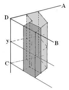
(a) (b)

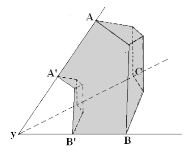
Figure 1. The dark area is $\Sigma_{y_{0}}\backslash\Sigma_{y_{0}}^{O}$ in a $3$-dimension $2P_{+}$. In (a), ${y_{0}}$ lies on two walls $ADC$ and $BDC$, $ADB$ is an outer face, the line segment $\overline{DC}$ stands for $I_{y_{0}}$, and the deeper dark area presents a subpolytope $P_{i}$ of case (2) in (a). In (b), ${y_{0}}$ lies on three walls.

Let $y=(y^{\prime},y^{\prime\prime})$ be any point in $\Sigma_{y_{0}}$. Fix a $y^{\prime\prime}\in I_{y_{0}}$. Since $u(y^{\prime},y^{\prime\prime})$ is a strictly convex function for $y^{\prime}$, by the $W$-invariance of $u$, it must attains its minima at $\tilde{y}_{0}=(y_{0}^{\prime},y^{\prime\prime})$, where ${y_{0}}^{\prime}$ is the coordinate component of ${y_{0}}$ in $U_{y_{0}}$. By the convexity of $u$, we have

$$\int_{\Sigma_{y_{0}}^{O}}u\,dy =\int_{I_{y_{0}}}\left(\int_{0}^{\frac{1}{2}}\int_{\partial U_{y_{0}}\backslash\tilde{W}_{k}}u(ty^{\prime},y^{\prime\prime})\langle y^{\prime},\nu\rangle\,d\sigma_{\partial U_{y_{0}}}(y^{\prime})\wedge dt\right)\wedge dy^{\prime\prime}$$

$$\leq\int_{I_{y_{0}}}\left(\int_{\frac{1}{2}}^{1}\int_{\partial U_{y_{0}}\backslash\tilde{W}_{k}}u(ty^{\prime},y^{\prime\prime})\langle y^{\prime},\nu\rangle\,d\sigma_{\partial U_{y_{0}}}(y^{\prime})\wedge dt\right)\wedge dy^{\prime\prime}$$

(4.19) $$=\int_{\Sigma_{y_{0}}\backslash\Sigma_{y_{0}}^{O}}u\,dy.$$

We divide ${\Sigma_{y_{0}}\backslash\Sigma_{y_{0}}^{O}}$ into finitely many subpolytopes $P_{1},...,P_{m}$ in two types:

• $P_{i}$ is contained in some $(2P^{\prime}_{+})_{\epsilon}$;

• $\bar{P_{i}}$ intersects at most $(k-1)$ Weyl walls and its outer faces are orthogonal to these walls.

For $P_{i}$ of type $(1)$, by (4.18), we have

(4.20) $$\int_{P_{i}}u\,dy\leq\epsilon^{-(n-r)}\int_{P_{i}}u\pi\,dy,~{}\forall u\geq 0.$$

For $P_{i}$ of type $(2)$, we regard $P_{i}$ as $\Sigma_{y^{(1)}}$ for some $y^{(1)}$ which lies on at most $(k-1)$ Weyl walls. Then according to the above argument, there is a subset $\Sigma_{y^{(1)}}^{O}$ of $\Sigma_{y^{(1)}}$ such that as in (4.3.1),

$$\int_{\Sigma_{y^{(1)}}^{O}}u\,dy\leq\int_{\Sigma_{y^{(1)}}\setminus\Sigma_{y^{(1)}}^{O}}u\,dy.$$

Moreover, we have finitely many subpolytopes $\{P_{j}^{(1)}\}_{j}$, where $P_{j}^{(1)}$ is either contained in some $(2P^{\prime}_{+})_{\epsilon_{1}}$ for some $\epsilon_{1}>0$, or intersects at most $(k-2)$ Weyl walls such that $\Sigma_{y^{(1)}}\setminus\Sigma_{y^{(1)}}^{O}=\cup_{j}P_{j}^{(1)}$.

Thus we can iterate the above progress for finite times until each $P_{j}^{(k)}$ in $\Sigma_{y^{(k)}}\setminus\Sigma_{y^{(k)}}^{O}$ is of type (1) for some $\epsilon_{k}>0$ while $P_{j}^{(k-1)}$ is of type (2). Hence by the relations (4.3.1) and (4.20), we can find a small number $\delta_{0}>0$ such that

$$\int_{\Sigma_{y_{0}}}u\,dy\leq C\delta_{0}^{-(n-r)}\int_{2P^{\prime}_{+}}u\pi\,dy.$$

Since $\partial(2P_{+})\cap(\cup_{\alpha\in\Phi_{+}}W_{\alpha})$ is compact, we can cover it by finitely many $\{\Sigma_{y_{p}}\}$. Choose $\epsilon_{0}>0$ such that $2P^{\prime}_{+}\setminus(2P^{\prime}_{+})_{\epsilon_{0}}\subset\cup_{p}\Sigma_{y_{p}}$. Then (4.16) follows from (4.18). ∎

Remark 4.7.

If $M$ is a toroidal compactification of $G$ [13], we can take $P^{\prime}=P$ and then Proposition 4.1 follows from Lemma 4.6 directly. Lemma 4.6 will be also used in Section 6 (cf. Lemma 6.1).

4.3.2. Asymptotic estimate of $Q$ near $W_{\alpha}$

In general, a Weyl wall $W_{\alpha}$ could not intersect a $(r-1)$-dimensional face $F_{\tilde{A}}$ of $2P$ orthogonally. In this case, if let $s_{\alpha}\in W_{\alpha}$ be the reflection with respect to $W_{\alpha}$, then by the $W$-invariance of $2P$, $F_{\tilde{A},\alpha}:=s_{\alpha}(F_{\tilde{A}})$ is again a face of $2P$. For simplicity, we denote $\mathfrak{F}_{\alpha}$

$$\mathfrak{F}_{\alpha}=\left\{F_{\tilde{A}}\subset\{y|~{}\langle\alpha,y\rangle\geq 0\}|~{}F_{\tilde{A}}\neq F_{\tilde{A},\alpha}\right\}.$$

We note that $F_{\tilde{A}}$ may not intersect $W_{\alpha}$.

In order to make the computation of the quantity $Q$ more explicitly, associated to each $W_{\alpha}$, we relabel the $(r-1)$-dimensional faces of $2P$ as follows:

1. Faces $F_{a}\in\mathfrak{F}_{\alpha}$. We denote them by $F_{a}=\{y\in\partial(2P)|~{}l_{a}(y)=0\},\,a=1,..,d_{1}$. By the convexity of $2P$, we have $\alpha(u_{a})>0$. Since $\alpha\in\mathfrak{M}$ and $u_{a}\in\mathfrak{N}$, $\alpha(u_{a})\in\mathbb{Z}_{>0}$.

2. Faces $F_{a,\alpha}$ with $F_{a}\in\mathfrak{F}_{\alpha}$. We denote them by $F_{a,\alpha}=\{y\in\partial(2P)|~{}l_{a,\alpha}(y)=0\}$, where $l_{a,\alpha}(y)$ satisfies

   (4.21) $$l_{a,\alpha}(y)=l_{a}(y)+{\frac{2\alpha(u_{a})}{|\alpha|^{2}}}\langle\alpha,y\rangle.$$

3. Faces $F_{b}$ which are orthogonal to $W_{\alpha}$. By the convexity of $2P$, $F_{b}\cap W_{\alpha}\neq\emptyset$. We denote them by $F_{b}=\{y\in\partial(2P)|~{}l_{b}(y)=0\},\,b=1,..,d_{2}$. Since $\alpha(u_{b})=0$, $F_{b}$ is invariant under $s_{\alpha}$.

Under the above notations, we rewrite Guillemin’s function $u_{0}$ in (2.3) as

$$u_{0}={\frac{1}{2}}\sum_{a}\left(l_{a}(y)\log l_{a}(y)+l_{a,\alpha}(y)\log l_{a,\alpha}(y)\right)+{\frac{1}{2}}\sum_{b}l_{b}(y)\log l_{b}(y).$$

Thus

(4.22) $$\langle\alpha,\nabla u_{0}\rangle={\frac{1}{2}}\sum_{a}\alpha(u_{a})\log\left(1+{\frac{2\alpha(u_{a})\alpha(y)}{|\alpha|^{2}l_{a}(y)}}\right)$$

and

(4.23) $${u_{0}}_{,ij}={\frac{1}{2}}\sum_{a}\left({\frac{u_{a}^{i}u_{a}^{j}}{l_{a}(y)}}+{\frac{u_{a,\alpha}^{i}u_{a,\alpha}^{j}}{l_{a,\alpha}(y)}}\right)+{\frac{1}{2}}\sum_{b}\left({\frac{u_{b}^{i}u_{b}^{j}}{l_{b}(y)}}\right).$$

Lemma 4.8.

Let $y_{0}\in W_{\alpha}$. Then

$$u_{0}^{ij}\alpha_{i}\alpha_{j}=\left\{\begin{aligned} &\left(\sum_{a}{\frac{(\alpha(u_{a}))^{2}}{l_{a}(y)}}\right)^{-1}|\alpha|^{4}+O(\alpha(y)),~{}\text{if }{\frac{\alpha(y)}{l_{a}(y)}\to 0},~{}\forall~{}a,\\[4.0pt] &O(\alpha(y)),~{}\text{otherwise}.\end{aligned}\right.$$

Proof.

Since $l_{a,\alpha}(y)>l_{a}(y)>0$, we have

$$0 <M_{1}:={\frac{1}{2}}\left[\sum_{a}{\frac{1}{l_{a,\alpha}(y)}}\left(u_{a}^{i}u_{a}^{j}+{u_{a,\alpha}^{i}u_{a,\alpha}^{j}}\right)+\sum_{b}{\frac{u_{b}^{i}u_{b}^{j}}{l_{b}(y)}}\right]$$

$$\leq(u_{0,ij})\leq{\frac{1}{2}}\left[\sum_{a}{\frac{1}{l_{a}(y)}}\left(u_{a}^{i}u_{a}^{j}+{u_{a,\alpha}^{i}u_{a,\alpha}^{j}}\right)+\sum_{b}{\frac{u_{b}^{i}u_{b}^{j}}{l_{b}(y)}}\right]=:M_{2}.$$

It is easy to see

(4.24) $$M_{1}\alpha=\left(\sum_{a}{\frac{(\alpha(u_{a}))^{2}}{|\alpha|^{2}l_{a,\alpha}(y)}}\right)\alpha,\ \ \ M_{2}\alpha=\left(\sum_{a}{\frac{(\alpha(u_{a}))^{2}}{|\alpha|^{2}l_{a}(y)}}\right)\alpha.$$

Thus

$$\left(\sum_{a}{\frac{(\alpha(u_{a}))^{2}}{l_{a}(y)}}\right)^{-1}={\frac{\alpha^{T}M_{2}^{-1}\alpha}{|\alpha|^{4}}}$$

$$\leq{\frac{u_{0}^{ij}\alpha_{i}\alpha_{j}}{|\alpha|^{4}}}\leq{\frac{\alpha^{T}M_{1}^{-1}\alpha}{|\alpha|^{4}}}=\left(\sum_{a}{\frac{(\alpha(u_{a}))^{2}}{l_{a}(y)+2{\frac{\alpha(u_{a})}{|\alpha|^{2}}}\alpha(y)}}\right)^{-1}.$$

Moreover, if ${\frac{\alpha(y)}{l_{a}(y)}}\to 0$ for all $a$, by Lemma 7.1 in Appendix,

$$0 \leq\left(\sum_{a}{\frac{(\alpha(u_{a}))^{2}}{l_{a}(y)+2{\frac{\alpha(u_{a})}{|\alpha|^{2}}}\alpha(y)}}\right)^{-1}-\left(\sum_{a}{\frac{(\alpha(u_{a}))^{2}}{l_{a}(y)}}\right)^{-1}$$

(4.25) $$=O(\alpha(y)).$$

This implies

$${\frac{u_{0}^{ij}\alpha_{i}\alpha_{j}}{|\alpha|^{4}}}\leq\left(\sum_{a}{\frac{(\alpha(u_{a}))^{2}}{l_{a}(y)}}\right)^{-1}+O(\alpha(y)).$$

The first case is proved.

In the second case, there exists an $F_{a_{0}}\in\mathfrak{F}_{\alpha}$ such that $\alpha(u_{a_{0}})\not=0$ and ${\frac{\alpha(y)}{l_{a_{0}}(y)}}\geq\epsilon_{0}$ for some $\epsilon_{0}>0$. Then

(4.26) $$\left(\sum_{a}{\frac{(\alpha(u_{a}))^{2}}{l_{a}(y)}}\right)^{-1}=O(l_{a_{0}}(y))$$

and

(4.27) $$\left(\sum_{a}{\frac{(\alpha(u_{a}))^{2}}{l_{a}(y)+2{\frac{\alpha(u_{a})}{|\alpha|^{2}}}\alpha(y)}}\right)^{-1}=O(\alpha(y)).$$

Thus

$${\frac{u_{0}^{ij}\alpha_{i}\alpha_{j}}{|\alpha|^{4}}}\leq O(l_{a_{0}}(y))+O(\alpha(y))=O(\alpha(y)).$$

The lemma is proved. ∎

Lemma 4.9.

Let $y_{0}\in W_{\alpha}$. Suppose that $y_{0}$ also lies on another Weyl wall $W_{\beta}$. Then as $y\to y_{0}$, it holds

(4.28) $$\alpha^{T}\left((u^{ij}_{0})-M_{2}^{-1}\right)\alpha= O(\alpha(y)),$$

(4.29) $$\beta^{T}\left((u^{ij}_{0})-M_{2}^{-1}\right)\beta=O(\alpha(y)+\beta(y)).$$

Proof.

(4.28) follows from the estimate in Lemma 4.8 immediately. It remains to prove (4.29). Let $S_{\alpha,\beta}\subset W$ be the group generated by the reflections $s_{\alpha}$ and $s_{\beta}$. We want to relabel faces of $2P$ according to this $S_{\alpha,\beta}$-action. In each orbit $\{S_{\alpha,\beta}F_{\tilde{A}}\}$, where $\{F_{\tilde{A}}\}$ is a $(r-1)$-dimensional face, we take a face $F_{c}$ such that $\alpha(u_{c}),\,\beta(u_{c})\geq 0$. Let

$$\{S_{\alpha,\beta}F_{c}\}=\{F_{c,s_{1}},...,F_{c,s_{p(c)}}\},$$

where $F_{c,s}=\{y\in\partial(2P)|~{}l_{c,s}(y)=\lambda_{c,s}-u_{c,s}^{i}y_{i}=0\}.$ Set

$$\hat{M}_{1}={\frac{1}{2}}\sum_{c}\left({\frac{\sum_{q=1}^{p(c)}u_{c,s_{q}}^{i}u_{c,s_{q}}^{j}}{\max_{s}\left\{\left(l_{c,s}\right)(y)\right\}}}\right),~{}\hat{M}_{2}={\frac{1}{2}}\sum_{c}\left({\frac{\sum_{q=1}^{p(c)}u_{c,s_{q}}^{i}u_{c,s_{q}}^{j}}{\min_{s}\left\{\left(l_{c,s}\right)(y)\right\}}}\right).$$

Then we rewrite $u_{0}$ as

$$u_{0}={\frac{1}{2}}\sum_{c}\sum_{q=1}^{p(c)}{\frac{u_{c,s_{q}}^{i}u_{c,s_{q}}^{j}}{l_{c,s_{q}}(y)}}.$$

Thus it is easy to see

$$0<\hat{M}_{1}\leq(u_{0,ij})\leq M_{2}\leq\hat{M}_{2}.$$

Note that $\{S_{\alpha,\beta}F_{c}\}$ is invariant under the reflection associated to $W_{\beta}$. Then as in the proof of Lemma 4.8, we relabel $\{S_{\alpha,\beta}F_{c}\}$: faces $F_{a}\in\mathfrak{F}_{\beta}$; faces $F_{a,\beta}$ with $F_{a}\in\mathfrak{F}_{\beta}$; and Faces $F_{b}$ which is orthogonal to $W_{\beta}$. Thus similar to (4.24), we get

$$\sum_{q=1}^{p(c)}u_{c,s_{q}}^{i}u_{c,s_{q}}^{j}\beta_{j}=\lambda_{c}\beta_{i},$$

where $\lambda_{c}\geq 0$ is a constant with at least one $\lambda_{c}>0$ since $\hat{M}_{1}>0$. As a consequence,

$$\hat{M}_{1}\beta={\frac{1}{2}}\sum_{c}\frac{\lambda_{c}}{\max_{s}\left\{l_{c,s}(y)\right\}}\beta$$

and

$$\hat{M}_{2}\beta={\frac{1}{2}}\sum_{c}\frac{\lambda_{c}}{\min_{s}\left\{l_{c,s}(y)\right\}}\beta.$$

This means that $\beta$ is an eigenvector of both $\hat{M}_{1}$ and $\hat{M}_{2}$.

On the other hand, there are constants $\mu_{1}^{c},\,\mu_{2}^{c}$ such that

$$l_{c,s}(y)=l_{c}(y)+\mu_{1}^{c}\alpha(y)+\mu_{2}^{c}\beta(y).$$

In particular,

$$\max_{s}\{l_{c,s}(y)\}=\min_{s}\{l_{c,s}(y)\}+\tilde{\mu}_{1}^{c}\alpha(y)+\tilde{\mu}_{2}^{c}\beta(y).$$

Then as in the estimate (4.3.2) (also see (4.26), (4.27)), we get

$$\beta^{T}\left(\hat{M}_{1}^{-1}-\hat{M}_{2}^{-1}\right)\beta=O(\alpha(y)+\beta(y)).$$

It follows

$$\beta^{T}\left((u^{ij}_{0})-M_{2}^{-1}\right)\beta=O(\alpha(y)+\beta(y)).$$

The lemma is proved.

∎

Remark 4.10.

Since (4.23) can be rewritten as

$${u_{0}}_{,ij}={\frac{1}{2}}\sum_{a}\left({\frac{u_{a}^{i}u_{a}^{j}}{l_{a}(y)}}+{\frac{u_{a,\beta}^{i}u_{a,\beta}^{j}}{l_{a,\beta}(y)}}\right)+{\frac{1}{2}}\sum_{b}\left({\frac{u_{b}^{i}u_{b}^{j}}{l_{b}(y)}}\right)$$

for any Weyl wall $W_{\beta}$, as in the proof of Lemma 4.8 for the second case, one can prove: if $y_{0}\notin W_{\beta}$, then

(4.30) $${u}^{ij}_{0}\beta_{i}\beta_{j}=O(1),~{}{\rm as}~{}y\to y_{0}.$$

Similar to (4.9),

(4.31) $$\beta^{T}\left((u^{ij}_{0})-M_{2}^{-1}\right)\beta=O(1),~{}{\rm if}~{}y_{0}\in W_{\alpha}\setminus W_{\beta}.$$

From (4.8), a direct computation shows

$$Q =\sum_{\alpha\in\Phi_{+}}\left[4{\frac{|\alpha|^{2}\coth\langle\alpha,\nabla u_{0}\rangle}{\alpha(y)}}-2{\frac{u_{0,ij}\alpha_{i}\alpha_{j}}{\sinh^{2}\langle\alpha,\nabla u_{0}\rangle}}-2u_{0}^{ij}{\frac{\alpha_{i}\alpha_{j}}{(\alpha(y))^{2}}}\right]$$

(4.32) $$+2\sum_{\alpha\neq\beta\in\Phi_{+}}\left[{\coth{\langle\alpha,\nabla u_{0}\rangle}}{\frac{\langle\alpha,\beta\rangle}{\beta(y)}}+{\coth{\langle\beta,\nabla u_{0}\rangle}}{\frac{\langle\alpha,\beta\rangle}{\alpha(y)}}-2u_{0}^{ij}{\frac{\alpha_{i}\beta_{j}}{\alpha(y)\beta(y)}}\right].$$

For simplicity, we denote each term in these two sums by $I_{\alpha}(y)$ and $I_{\alpha,\beta}(y)$, respectively. We need to estimate them in the following key lemma.

Lemma 4.11.

Let $y_{0}\in W_{\alpha}$. Then there exist $C_{\alpha,y_{0}},C_{\alpha,\beta,y_{0}}>0$, such that

(4.33) $$|I_{\alpha}(y)|\leq{\frac{C_{\alpha,y_{0}}}{\alpha(y)}}$$

and

(4.34) $$|I_{\alpha,\beta}(y)|\leq C_{\alpha,\beta,y_{0}}\left({\frac{1}{\alpha(y)}}+{\frac{1}{\beta(y)}}\right)$$

as $y\to y_{0}$.

Proof.

We consider the following three cases as $y\to y_{0}$:

• ${\frac{\alpha(y)}{l_{a}(y)}}\leq\epsilon_{0}<<1$, $\forall F_{a}\in\mathfrak{F}_{\alpha}$.

• There is an $F_{a_{0}}\in\mathfrak{F}_{\alpha}$ such that $0<{\frac{1}{\tau}}<{\frac{\alpha(y)}{l_{a_{0}}(y)}}<\tau$ for some $0<\tau<+\infty$, and ${\frac{\alpha(y)}{l_{a}(y)}}\leq\tau,~{}\forall F_{a}$.

• There is an $F_{a_{0}}\in\mathfrak{F}_{\alpha}$ such that ${\frac{\alpha(y)}{l_{a_{0}}(y)}}\geq N_{0}>>1$.

Case (i). In this case, $\langle\alpha,\nabla u_{a}\rangle\to 0$. By (4.22), it is easy to check

$$\langle\alpha,\nabla u_{0}\rangle=\sum_{a}{\frac{(\alpha(u_{a}))^{2}\alpha(y)}{|\alpha|^{2}l_{a}(y)}}+O\left(\sum_{a}\left({\frac{(\alpha(u_{a}))^{2}\alpha(y)}{|\alpha|^{2}l_{a}(y)}}\right)^{2}\right).$$

Then

$$\coth\langle\alpha,\nabla u_{0}\rangle = {\frac{|\alpha|^{2}}{\alpha(y)}}\left(\sum_{a}{\frac{(\alpha(u_{a}))^{2}}{l_{a}(y)}}\right)^{-1}+O(1).$$

On the other hand, by (4.23), one can show

$$u_{0,ij}\alpha_{i}\alpha_{j}=\left(\sum_{a}{\frac{(\alpha(u_{a}))^{2}}{l_{a}(y)}}\right)+O\left(\sum_{a}{\frac{\alpha(y)}{l_{a}(y)l_{a,\alpha}(y)}}\right).$$

Then

$${\frac{u_{0,ij}\alpha_{i}\alpha_{j}}{\sinh^{2}\langle\alpha,\nabla u_{0}\rangle}}={\frac{|\alpha|^{4}}{(\alpha(y))^{2}}}\left(\sum_{a}{\frac{(\alpha(u_{a}))^{2}}{l_{a}(y)}}\right)^{-1}+O\left({\frac{1}{\alpha(y)}}\right).$$

Thus

$$4{\frac{|\alpha|^{2}\coth\langle\alpha,\nabla u_{0}\rangle}{\alpha(y)}}-2{\frac{u_{0,ij}\alpha_{i}\alpha_{j}}{\sinh^{2}\langle\alpha,\nabla u_{0}\rangle}}$$

$$=2{\frac{|\alpha|^{4}}{(\alpha(y))^{2}}}\left(\sum_{a}{\frac{(\alpha(u_{a}))^{2}}{l_{a}(y)}}\right)^{-1}+O\left({\frac{1}{\alpha(y)}}\right).$$

Hence, by the above relation and Lemma 4.8, we see that there exists a constant $C^{\prime}>0$ such that $|I_{\alpha}(y)|\leq{\frac{C^{\prime}}{\alpha(y)}}$.

Case (ii). In this case, it is easy to see

$$0<\coth\langle\alpha,\nabla u_{0}\rangle,\,\frac{1}{\sinh^{2}\langle\alpha,\nabla u_{0}\rangle}\leq C^{\prime}_{\tau},~{}{\rm and}~{}u_{0,ij}\alpha_{i}\alpha_{j}=O\left(\frac{1}{\alpha(y)}\right).$$

Then by Lemma 4.8, we have $|I_{\alpha}(y)|\leq{\frac{C_{\tau}}{\alpha(y)}}$, where the constant $C_{\tau}<\infty$ depends only on $\tau$.

Case (iii). In this case, we may assume

$$\frac{\alpha(y)}{l_{a}(y)}\leq\frac{\alpha(y)}{l_{a_{0}}(y)}\geq N_{0},~{}\forall a=1,...,d_{1}.$$

Then by (4.22), we have

(4.35) $$\langle\alpha,\nabla u_{0}\rangle\geq{\frac{1}{2}}\alpha(u_{a_{0}})\log\left(1+{\frac{2\alpha(u_{a_{0}})\alpha(y)}{|\alpha|^{2}l_{a_{0}}(y)}}\right).$$

It follows

(4.36) $$\coth\langle\alpha,\nabla u_{0}\rangle=O(1)$$

and

$$\sinh^{2}\langle\alpha,\nabla u_{0}\rangle\geq\left(1+{\frac{2\alpha(u_{a_{0}})\alpha(y)}{|\alpha|^{2}l_{a_{0}}(y)}}\right)^{\alpha(u_{a_{0}})}.$$

On the other hand, by (4.23), it is easy to see

$$u_{0,ij}\alpha_{i}\alpha_{j}\leq 2d_{1}\left({\frac{(\alpha(u_{a_{0}})^{2})}{l_{a_{0}}(y)}}\right)+C.$$

Thus

(4.37) $${\frac{u_{0,ij}\alpha_{i}\alpha_{j}}{\sinh^{2}\langle\alpha,\nabla u_{0}\rangle}}=O\left({\frac{1}{\alpha(y)}\left({\frac{l_{a_{0}}(y)}{\alpha(y)}}\right)^{\alpha(u_{a_{0}})-1}}\right)\leq o\left({\frac{1}{\alpha(y)}}\right).$$

Here we used the fact that $\alpha(u_{a})\in\mathbb{Z}_{>0}$, hence $\geq 1$. Hence, combining (4.36) and (4.37) together with Lemma 4.8, we get $I_{\alpha}(y)=O\left(\frac{1}{\alpha(y)}\right)$. The proof of (4.33) is completed.

Next, we prove (4.34). We may assume $y_{0}\in W_{\alpha}\cap W_{\beta}$, otherwise, (4.34) can be more easy to obtained (cf. Remark 4.10). We note that $(u_{0}^{ij})-M_{2}^{-1}\geq 0$ and $\alpha$ is an eigenvector of $M_{2}$. Then by the above discussion for $\coth\langle\alpha,\nabla u_{0}\rangle$ in cases (i)-(iii), we have

$$\coth\langle\alpha,\nabla u_{0}\rangle\cdot\langle\alpha,\beta\rangle-{\frac{\langle M_{2}^{-1}\alpha,\beta\rangle}{\alpha(y)}}=O(1).$$

On the other hand, by Lemma 4.9,

$$\left|{\frac{\alpha^{T}((u_{0}^{ij})-M_{2}^{-1})\beta}{\alpha(y)}}\right|\leq{\frac{O(\alpha(y)+\beta(y))}{\alpha(y)}}.$$

Thus

$$\coth{\langle\alpha,\nabla u_{0}\rangle}{\frac{\langle\alpha,\beta\rangle}{\beta(y)}}-u_{0}^{ij}{\frac{\alpha_{i}\beta_{j}}{\alpha(y)\beta(y)}}=O\left({\frac{1}{\alpha(y)}}+{\frac{1}{\beta(y)}}\right),~{}y\to y_{0}.$$

Similarly, we have

$$\coth{\langle\beta,\nabla u_{0}\rangle}{\frac{\langle\alpha,\beta\rangle}{\alpha(y)}}-u_{0}^{ij}{\frac{\alpha_{i}\beta_{j}}{\alpha(y)\beta(y)}}=O\left({\frac{1}{\alpha(y)}}+{\frac{1}{\beta(y)}}\right),~{}y\to y_{0}.$$

Combining these two relations, we see that (4.34) is true. ∎

By Lemma 4.6 and Lemma 4.11, we begin to prove Proposition 4.5.

Proof of Proposition 4.5.

Set a compact subset of $\partial(2P_{+})$ by

$$\Omega^{*}=\cup_{\alpha\in\Phi_{+}}\{y\in W_{\alpha}\cap F_{\tilde{A}}|~{}W_{\alpha}~{}{\rm intersects}~{}F_{\tilde{A}}~{}{\rm not~{}orthogonally}\}.$$

Since $\emptyset\neq F_{\tilde{A}}\cap F_{\tilde{A},\alpha}\subset W_{\alpha}$ if $F_{\tilde{A}}\cap W_{\alpha}\neq\emptyset$, each point in $\Omega^{*}$ lies on a face of codimension greater than 2. We claim: for any $y_{0}\in\Omega^{*}\cap\overline{(2P_{+})}$, there is a neighbourhood $V_{y_{0}}$ and a constant $C_{y_{0}}>0$ such that

(4.38) $$|Q|\leq C_{y_{0}}\left\langle\rho,{\frac{\nabla\pi}{\pi}}\right\rangle,\ \forall y\in V_{y_{0}}\cap(2P_{+}).$$

By (2.4), we see there exists a uniform $C$ such that

$$\left\langle{\frac{\nabla\pi}{2\pi}},\rho\right\rangle=\sum_{\alpha\in\Phi_{+}}{\frac{\langle\alpha,\rho\rangle}{\alpha(y)}}\geq C\sum_{\alpha\in\Phi_{+}}{\frac{1}{\alpha(y)}},$$

since $\langle\alpha,\rho\rangle>0$ for each $\alpha$. Thus by Lemma 4.11, to prove the claim, it suffices to estimate $I_{\beta}(y)$ with $y_{0}\notin W_{\beta}$ and $I_{\beta,\gamma}(y)$ with $y_{0}\notin W_{\beta}\cup W_{\gamma}$. The later can be easily settled. In fact, $I_{\beta,\gamma}(y)$ is bounded near $y_{0}$. For $I_{\beta}(y)$, we observe that $\langle\beta,\nabla u_{0}\rangle\geq C_{0}>0$ for any $y\in V_{y_{0}}$. As in the proof of Lemma 4.11 for Case (iii), we have

$$\coth\langle\beta,\nabla u_{0}\rangle=O(1)$$

and

$${\frac{u_{0,ij}\beta_{i}\beta_{j}}{\sinh^{2}\langle\beta,\nabla u_{0}\rangle}}=O\left({\frac{1}{\beta(y)}\left({\frac{l_{a_{0}}(y)}{\beta(y)}}\right)^{\beta(u_{a_{0}})-1}}\right)\leq O(1).$$

Hence, together with (4.30) in Remark 4.10, we get

(4.39) $$|I_{\beta}(y)|\leq C,~{}\forall y\in V_{y_{0}}\cap(2P_{+}).$$

The claim is proved.

By the above claim, we can pick a small neighbourhood $U$ of $\bar{\Omega}^{*}$ in $2P$ and a constant $C_{U}<+\infty$ independent of $u$, such that

(4.40) $$|Q|\leq C_{U}\left\langle\rho,{\frac{\nabla\pi}{\pi}}\right\rangle,\,\ \forall y\in U\cap(2P_{+}).$$

Furthermore, we can take a $W$-invariant polytope $P^{\prime}$ whose boundary intersects the Weyl walls orthogonally and $2P\backslash 2P^{\prime}\subset U$. This can be done as follows: for any $F_{\tilde{A}}\cap W_{\alpha_{(1)}}\cap...\cap W_{\alpha_{(k)}}\subset\Omega^{*}$, we chop off a sufficiently small corner of $2P$ with $F_{\tilde{A}}\cap W_{\alpha_{(1)}}\cap...\cap W_{\alpha_{(k)}}$ being the top and with the base lying on an $(r-1)$-plane which is parallel to $F_{\tilde{A}}\cap W_{\alpha_{(1)}}\cap...\cap W_{\alpha_{(k)}}$ and orthogonal to $W_{\alpha_{(1)}},...,W_{\alpha_{(k)}}$. By suitable choice of the chopping off, $2P^{\prime}$ is $W$-invariant (See Figure 2).

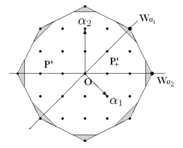
(a) (b)

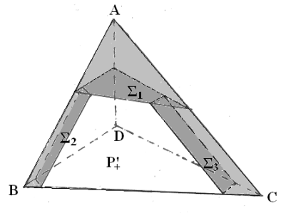
Figure 2. The dark areas stand for $U$. In (a), $P$ is of dimension $2$ and we present out the whole $P$ and $U$. In (b), $P$ is of dimension $3$. We only present out $P_{+}$. $ADB,~{}ADC$ are two walls and $ABC,~{}BDC$ are outer faces. For simplicity, we assume that $BDC$ is orthogonal to both walls, so that we need not to cut $P_{+}$ near $\overline{BD}$ and $\overline{CD}$.

Note that $|Q\pi|$ is uniformly bounded on $2P$. Thus by Lemma 4.6 and (4.40), we obtain

$$\left|\int_{2P_{+}}Qu\pi\,dy\right| \leq\left(\int_{U}+\int_{{2P^{\prime}_{+}}}\right)|Qu\pi|dy$$

$$\leq C_{U}\int_{2P_{+}}\langle\rho,{\nabla\pi}\rangle u\,dy+\hat{C}\int_{{2P^{\prime}_{+}}}u\pi dy.$$

Proposition 4.5 is proved. ∎

Remark 4.12.

According to the proof in Lemma 4.11, we actually prove that (4.38) holds for any $y_{0}\in\overline{2P_{+}}$. Then we can avoid to use Lemma 4.6 and improve Proposition 4.5 by the following estimate

$$\left|\int_{2P_{+}}Qu\pi\,dy\right|\leq C\int_{2P_{+}}\langle\rho,{\nabla\pi}\rangle u\,dy,~{}\forall u\in\hat{\mathcal{C}}_{\infty,W}.$$

Proof of Proposition 4.1.

Let $f(t)=t-\log\sinh t,\,t>0$. Then

$$0>f(t)-f(\epsilon t)>\log\epsilon.$$

Regarding $\mathcal{N}(\cdot)$ as $f(t)$, and then by Proposition 4.4, it follows

(4.41) $$\mathcal{N}(u)>\mathcal{N}(\epsilon u)-n\log\epsilon\geq C_{0}-\epsilon\mathcal{L}_{B}(u)-n\log\epsilon,$$

where

$$\mathcal{L}_{B}(u)=-C_{\Lambda}\int_{\partial(2P_{+})}u\langle y,\nu\rangle\pi\,d\sigma_{0}-C_{L}\mathcal{L}(u)+\int_{2P_{+}}Qu\pi\,dy.$$

On the other hand, by Lemma 4.2 and Propositions 4.3 and 4.5, for any $\delta\in(0,1)$, there exists uniform constants $C_{1}$, $C_{2}$, $C_{3}$ independent of $u$ such that

$$\mathcal{L}_{B}(u)-\mathcal{L}(u) \leq C_{1}\int_{(2P_{+})}u\pi\,dy+C_{2}\int_{\partial(2P_{+})}u\langle y,\nu\rangle\pi\,d\sigma_{0}+C_{3}\mathcal{L}(u)$$

$$\leq\left(C_{1}\Lambda+C_{2}\right)\int_{\partial{(2P_{+})}}u\langle y,\nu\rangle\pi\,d\sigma_{0}+C_{3}\mathcal{L}(u)$$

$$\leq\left(C_{1}\Lambda+C_{2}+\delta\Lambda\right)\int_{\partial{(2P_{+})}}u\langle y,\nu\rangle\pi\,d\sigma_{0}+C_{3}\mathcal{L}(u)-\delta\int_{2P_{+}}u\pi\,dy$$

(4.42) $$\leq\left(C_{3}+{\frac{C_{1}\Lambda+C_{2}+\delta\Lambda}{\lambda}}\right)\mathcal{L}(u)-\delta\int_{2P_{+}}u\pi\,dy.$$

Thus by choosing $\epsilon=\left[1+\left(C_{3}+{\frac{C_{1}\Lambda+C_{2}+\delta\Lambda}{\lambda}}\right)\right]^{-1}$, we get

$$\mathcal{L}_{B}(\epsilon u)<\mathcal{L}(u)-\epsilon\delta\int_{2P_{+}}u\pi\,dy.$$

By (4.41), we derive

$$\mathcal{K}(u)\geq\epsilon\delta\int_{2P_{+}}u\pi\,dy-C_{\delta},$$

where $C_{\delta}$ is independent of $u$. (4.3) is proved by replacing $\epsilon\delta$ with $\delta$. ∎

4.4. Proof of Theorem 1.2

Recall that the $J$-functional is given by

$$J_{\omega_{0}}(\phi) ={\frac{1}{V_{M}}}\int_{0}^{1}\int_{M}\dot{\phi}_{t}(\omega_{0}^{n}-\omega_{\phi_{t}}^{n})\wedge dt,$$

where $\phi\in\mathcal{H}_{K\times K}(\omega_{0})$ and $\phi_{t}$ is a path in $\mathcal{H}_{K\times K}(\omega_{0})$ joining $0$ and $\phi$. The following definition can be found in [24, 33, 15], etc.

Definition 4.13.

$\mu_{\omega_{0}}(\phi)$ is called proper modulo a subgroup $G_{0}$ of $\text{Aut}(M)$ in Kähler class $[\omega_{0}]$ if there is a continuous function $p(t)$ on $\mathbb{R}$ with the property $\displaystyle\lim_{t\to+\infty}p(t)=+\infty$, such that

$$\mu_{\omega_{0}}(\phi)\geq\inf_{\sigma\in G_{0}}p(J_{\omega_{0}}(\phi_{\sigma})),$$

where $\phi_{\sigma}$ is defined by $\omega_{0}+\sqrt{-1}\partial\bar{\partial}\phi_{\sigma}=\sigma^{*}(\omega_{0}+\sqrt{-1}\partial\bar{\partial}\phi).$

For our purpose, we focus on $\phi\in\mathcal{H}_{K\times K}(\omega_{0})$ and $G_{0}=Z(G)$. Let $u$ be the Legendre function of $\psi_{0}+\phi$. Take a $v\in\eta_{c}(M)$ such that Re$(v)=-\nabla u(O)$. Let $\sigma_{t}^{v}$ be a one parameter group generated by Re$(v)$. Then $(\sigma_{t}^{v})\in Z(G)$. It follows

$$(\sigma^{v}_{1})^{*}\omega_{\phi}=\omega_{0}+\sqrt{-1}\partial\bar{\partial}\tilde{\phi}$$

induces a $K\times K$-invariant Kähler potential $\tilde{\phi}$. Thus the Legendre function $\tilde{u}$ of $\psi_{0}+\tilde{\phi}$ satisfies $\nabla\tilde{u}(O)=0$. Moreover, $\nabla(\psi_{0}+\tilde{\phi})(O)=0$. Since we may also normalize $\psi_{0}+\tilde{\phi}$ so that $(\psi_{0}+\tilde{\phi})(O)=0$, thus $\tilde{u}(O)=0$. Moreover, $\mathcal{K}(\tilde{u})=\mathcal{K}(u)$ since $\mathcal{L}(\tilde{u})=\mathcal{L}(u)$ by Lemma 3.2 and the vanishing of Futaki invariant.

The following lemma is an analogue to [33, Lemma 2.2].

Lemma 4.14.

There exists a uniform $C_{J}>0$ such that

$$\left|J_{\omega_{0}}(\tilde{\phi})-{\frac{1}{V}}\int_{2P_{+}}\tilde{u}\pi\,dy\right|\leq C_{J},\ \forall\phi\in\mathcal{H}_{K\times K}(\omega_{0}),$$

where $\tilde{u}\in\hat{\mathcal{C}}_{\infty,W}$ and $\psi_{0}+\tilde{\phi}$ is the Legendre function of $\tilde{u}$.

Proof.

In fact, Lemma 4.14 comes from the following new version of $\mathcal{J}_{\omega_{0}}(\phi)$,

$$J_{\omega_{0}}(\phi) = {\frac{1}{V_{M}}}\int_{M}\phi\,\omega_{0}^{n}-{\frac{1}{V_{M}}}\int_{0}^{1}\int_{M}\dot{\phi}_{t}\,\omega_{\phi_{t}}^{n}\wedge dt$$

$$= {\frac{1}{V_{M}}}\int_{M}\phi\,\omega_{0}^{n}-{\frac{1}{V}}\int_{0}^{1}\int_{\mathfrak{a}_{+}}\dot{\phi_{t}}MA_{\mathbb{R}}(\psi_{t})\prod_{\alpha\in\Phi_{+}}\langle\alpha,\nabla\psi_{t}\rangle^{2}\,dx\wedge dt$$

$$= {\frac{1}{V_{M}}}\int_{M}\phi\,\omega_{0}^{n}+{\frac{1}{V}}\int_{2P_{+}}(u-u_{0})\pi\,dy.$$

Then the lemma can be proved similarly as Lemma 2.2 in [33]. ∎

Proof of Theorem 1.2.

For any $\phi\in\mathcal{H}_{K\times K}(\omega_{0})$, there exists $\sigma\in Z(G)$ such that

$$\sigma^{*}\omega_{\phi}=\omega_{0}+\sqrt{-1}\partial\bar{\partial}\tilde{\phi}$$

as above. Applying Proposition 4.1, we have

$$\mathcal{K}(\tilde{u})\geq\delta\int_{2P_{+}}\tilde{u}\pi dy-C_{\delta}.$$

Thus by Proposition 3.1 and Lemma 4.14, we get

$$\mu_{\omega_{0}}(\phi)=\mu_{\omega_{0}}(\phi)=\frac{1}{V}\mathcal{K}(\tilde{u})\geq\delta\cdot J_{\omega_{0}}(\tilde{\phi})-C_{J}-{\frac{C_{\delta}}{V}}.$$

The theorem is proved. ∎

5. Kähler-Ricci solitons and the Modified K-energy

In this section, we verify the properness of modified K-energy on $(M,K_{M}^{-1})$ under an analogous condition of (1.1). By Hodge theorem, for any $v\in\eta(M)$, there exists a unique smooth complex-valued function $\theta_{v}(\omega_{\phi})$ of $M$ such that

$$i_{v}\omega_{\phi}=\sqrt{-1}\bar{\partial}\theta_{v}(\omega_{\phi}),\ \int_{M}e^{\theta_{v}(\omega_{\phi})}\omega_{\phi}^{n}=\int_{M}\omega_{\phi}^{n}.$$

If $\phi\in\mathcal{H}_{K\times K}(\omega_{0})$ and $v\in\eta_{c}(M)$, $\theta_{v}(\omega_{\phi})$ is $K\times K$-invariant, so it can be written as

$$\theta_{X}(\omega_{\phi})=c^{i}{\frac{\partial\psi}{\partial x^{i}}}+c,~{}\forall x\in\mathfrak{a},$$

where $c^{i}$ and $c$ are constants with $c^{i}\alpha_{i}=0$ for any $\alpha\in\Phi_{+}$. Since the soliton vector field $X\in\eta_{c}(M)$ and Im$(X)\in\mathfrak{k}_{r}$, we have $c^{i},\,c\in\mathbb{R}$. Furthermore, by the vanishing of the modified Futaki invariant [27], they can be uniquely determined by the following linear equations,

$$\int_{2P_{+}}(c^{i}y_{i}+c)\pi\,dy = 0,$$

(5.1) $$\left\langle v,\int_{2P_{+}}ye^{c^{i}y_{i}+c}\pi\,dy\right\rangle = 0,\ \ \ \forall v\in\mathfrak{a}^{*}_{t}.$$

The modified K-energy $\mu_{\omega_{0}}^{X}(\cdot)$ associated to $X$ is defined by

$$\mu_{\omega_{0}}^{X}(\phi)={\frac{1}{V_{M}}}\int_{M}\log{\left({\frac{\omega_{\phi}^{n}}{\omega_{0}^{n}}}e^{\phi-h_{0}}\right)}e^{\theta_{X}(\omega_{\phi})}\omega_{\phi}^{n}-{\frac{1}{V_{M}}}\int_{0}^{1}\int_{M}\dot{\phi_{t}}e^{\theta_{X}(\omega_{\phi_{t}})}\omega_{\phi_{t}}^{n}\wedge dt,$$

where $\phi\in\mathcal{H}_{X}(\omega_{0})$ and $\phi_{t}$ is a path in $\mathcal{H}_{X}(\omega_{0})$ joining 0 and $\phi$ [27]. The modified J-functional is defined by

$$J_{\omega_{0}}^{X}(\phi)={\frac{1}{V_{M}}}\int_{0}^{1}\int_{M}\dot{\phi}_{t}\left(e^{\theta_{X}(\omega_{0})}\omega_{0}^{n}-e^{\theta_{X}(\omega_{\phi_{t}})}\omega_{\phi_{t}}^{n}\right)\wedge dt.$$

The properness of $\mu_{\omega_{0}}^{X}(\cdot)$ can be defined analogous to Definition 4.13 [9].

The following is the main result of this section.

Theorem 5.1.

Let $M$ be a Fano compactification of $G$ and $X$ the soliton vector field as above. Let

$$bar_{X}:={\frac{\int_{2P_{+}}ye^{\theta_{X}(y)}\pi\,dy}{\int_{2P_{+}}e^{\theta_{X}(y)}\pi\,dy}},$$

where $\theta_{X}(y)=c^{i}y_{i}+c$. Suppose that the corresponding polytope $2P_{+}$ satisfies

(5.2) $$bar_{X}\in 4\rho+\Xi.$$

Then $\mu_{\omega_{0}}^{X}(\cdot)$ is proper on $\mathcal{H}_{K\times K}(\omega_{0})$ modulo $Z(G)$.

Since the properness of the modified K-energy implies the existence of Kähler-Ricci solitons [28], Theorem 5.1 gives a proof for the existence of Kähler-Ricci solitons under the condition (5.2). As in the proof of Proposition 3.4, one can also show that (5.2) is a necessary condition by using the computation as for toric manifolds [30].

5.1. Reduction of Modified K-energy

The following is a generalization of Proposition 3.1 in [30].

Proposition 5.2.

Let $\phi\in\mathcal{H}_{K\times K}(\omega_{0})$ and $u$ be the Legendre function of $\psi=\psi_{0}+\phi$. Then

$$\mu_{\omega_{0}}^{X}(\phi)=\frac{1}{V}\mathcal{K}^{X}(u)+const.,$$

where $\mathcal{K}^{X}(u)=\mathcal{N}^{X}(u)+\mathcal{L}^{X}(u)$, and

$$\mathcal{L}^{X}(u)=\int_{2P_{+}}\langle y-4\rho,\nabla u\rangle e^{\theta_{X}(y)}\pi\,dy,.$$

(5.3) $$\mathcal{N}^{X}(u)=-\int_{2P_{+}}\left(\log\det\left(u_{ij}\right)-\chi\left(\nabla u\right)-4\langle\rho,\nabla u\rangle\right)e^{\theta_{X}(y)}\pi\,dy.$$

Proof.

By (2.2) and (3.12), we reduce ${\frac{\omega_{\phi}^{n}}{\omega_{0}^{n}}}e^{\phi-h_{0}}$ to a function on $\mathfrak{a}_{+}$ by

$$\frac{\omega_{\phi}^{n}}{\omega_{0}^{n}}e^{\phi-h_{0}}=\frac{MA_{\mathbb{R}}(\psi)\prod_{\alpha\in\Phi_{+}}\langle\alpha,\nabla\psi\rangle^{2}}{J(x)}e^{\psi}.$$

Then

$$\ \ \ {\frac{1}{C_{H}}}\int_{M}\log\left({\frac{\omega_{\phi}^{n}}{\omega_{0}^{n}}e^{\phi-h_{0}}}\right)e^{\theta_{X}(\omega_{\phi})}\,\omega_{\phi}^{n}$$

$$=\int_{\mathfrak{a}_{+}}\left[\log MA_{\mathbb{R}}(\psi)+\psi+\chi(x)\right]e^{\theta_{X}(y)}MA_{\mathbb{R}}(\psi)\prod_{\alpha\in\Phi_{+}}\langle\alpha,\nabla\psi\rangle^{2}dx+C_{\pi}$$

$$=\int_{2P_{+}}\left[-\log\det(u_{,ij})+\chi(\nabla u)\right]e^{\theta_{X}(y)}\pi\,dy$$

(5.4) $$\ \ \ +\int_{\mathfrak{a}_{+}}\psi e^{\theta_{X}(y)}MA_{\mathbb{R}}(\psi)\prod_{\alpha\in\Phi_{+}}\langle\alpha,\nabla\psi\rangle^{2}dx+C_{\pi},$$

where $C_{\pi}=\int_{2P_{+}}\log\pi(y)\cdot e^{\theta_{X}(y)}\pi\,dy$ is a uniform constant. On the other hand,

$$\ \ \ -{\frac{1}{C_{H}}}\int_{0}^{1}\int_{M}\dot{\phi}_{t}e^{\theta_{X}(\omega_{\phi_{t}})}\omega_{\phi_{t}}^{n}\wedge dt$$

$$=-\int_{0}^{1}\int_{\mathfrak{a}_{+}}\dot{\phi}_{t}e^{\theta_{X}(y)}MA_{\mathbb{R}}(\psi_{t})\prod_{\alpha\in\Phi_{+}}\langle\alpha,\nabla\psi_{t}\rangle^{2}dx\wedge dt$$

$$=\int_{2P_{+}}ue^{\theta_{X}(y)}\pi\,dy-\int_{2P_{+}}u_{0}e^{\theta_{X}(y)}\pi\,dy$$

$$=\int_{\mathfrak{a}_{+}}\left(x^{i}{\frac{\partial\psi}{\partial x^{i}}}-\psi\right)e^{\theta_{X}(y)}MA_{\mathbb{R}}(\psi)\prod_{\alpha\in\Phi_{+}}\langle\alpha,\nabla\psi\rangle^{2}dx+C.$$

Combining this with (5.4), we get

$$\mu_{\omega_{0}}^{X}(\phi) ={\frac{1}{V}}\int_{2P_{+}}\langle y,\nabla u\rangle e^{\theta_{X}(y)}\pi\,dy$$

$$\ \ +{\frac{1}{V}}\left(\int_{2P_{+}}\chi\left(\nabla u\right)e^{\theta_{X}(y)}\pi\,dy-\int_{2P_{+}}\log\det\left(u_{,ij}\right)e^{\theta_{X}(y)}\pi\,dy\right)+const.$$

This proves the proposition. ∎

5.2. Properness

Analogous to Proposition 4.3, we have

Proposition 5.3.

Under $(\ref{bar4})$, it holds

(5.5) $$\mathcal{L}^{X}(u)\geq\lambda_{X}\int_{\partial(2P_{+})}u\langle y,\nu\rangle e^{\theta_{X}(y)}\pi\,d\sigma_{0},~{}\forall u\in\hat{\mathcal{C}}_{\infty,+},$$

where $\lambda_{X}>0$ is a uniform constant.

Proof.

By (5.2), we have

$$\langle bar_{X}-4\rho,\nabla u\rangle\geq 0,~{}\forall y\in 2P_{+}.$$

Then

$$\mathcal{L}^{X}(u)\geq\int_{2P_{+}}\langle y-bar_{X},\nabla u\rangle e^{\theta_{X}(y)}\pi\,dy.$$

On the other hand, by the convexity of $u$, we have

$$\langle y-bar_{X},\nabla u\rangle\geq u(y)-u(bar_{X})\geq\langle y-bar_{X},\nabla u|_{bar_{X}}\rangle.$$

Thus

$$\mathcal{L}^{X}(u)\geq\int_{2P_{+}}\langle y-bar_{X},\nabla u|_{bar_{X}}\rangle e^{\theta_{X}(y)}\pi\,dy=0.$$

Now we can follow the arguments in the proof of Proposition 4.3 to get (5.5). ∎

Proposition 5.4.

Under (5.2), for any $\delta\in(0,1)$, there exists a uniform constant $C_{\delta}>0$ such that

(5.6) $$\mathcal{K}^{X}(u)\geq\delta\int_{2P_{+}}ue^{\theta_{X}(y)}\pi\,dy-C_{\delta},~{}\forall u\in\hat{\mathcal{C}}_{\infty,+}.$$

Proof.

Since $-\log\det$ and $\chi(x)$ are both convex, by (5.3), we have

$$\mathcal{N}^{X}(u)\geq\int_{2P_{+}}\left(\left.{\frac{\partial\chi}{\partial x^{i}}}\right|_{x=\nabla u_{0}}+4\rho_{i}\right)u_{,i}e^{\theta_{X}(y)}\pi\,dy-\int_{2P_{+}}u_{0}^{ij}u_{,ij}e^{\theta_{X}(y)}\pi\,dy+C_{0}.$$

By integration by parts, we get an analogue of (4.2),

$$\mathcal{N}^{X}(u)\geq -\sum_{A}\int_{F_{A}}{\frac{2}{\lambda_{A}}}\langle y,\nu_{A}\rangle ue^{\theta_{X}(y)}\pi\,d\sigma_{0}$$

$$-\int_{2P_{+}}\left(u^{ij}_{0,ij}+u_{0}^{ij}c^{i}c^{j}+2u_{0,j}^{ij}c^{i}\right)ue^{\theta_{X}(y)}\pi\,dy$$

(5.7) $$-\int_{2P_{+}}2\left(u_{0,j}^{ij}+u_{0}^{ij}c^{j}\right)\pi_{,i}e^{\theta_{X}(y)}udy+\int_{2P_{+}}Que^{\theta_{X}(y)}\pi dy.$$

Here we used the fact that

$$\left(\left.{\frac{\partial\chi}{\partial x^{i}}}\right|_{x=\nabla u_{0}}+4\rho_{i}\right)\pi(y)=0,~{}\forall y\in\partial(2P^{+})$$

and

$$c^{i}{\frac{\partial\chi}{\partial x^{i}}}(x)+4c^{i}\rho_{i}=-2\sum_{\alpha\in\Phi_{+}}c^{i}\alpha_{i}\cdot\coth x+4c^{i}\rho_{i}=0.$$

On the other hand, $\mathcal{L}^{X}(u)$ can be rewritten as

$$\mathcal{L}^{X}(u)=\int_{\partial(2P_{+})}\langle y-4\rho,\nu\rangle ue^{\theta_{X}(y)}\pi\,d\sigma_{0}-\int_{2P_{+}}[n+c^{i}(y_{i}-4\rho_{i})]ue^{\theta_{X}(y)}\pi\,dy.$$

Note that $\theta_{X}(y)$ is uniformly bounded on $2P^{+}$. Then we have

$$\int_{2P_{+}}\langle\rho,{\nabla\pi}\rangle ue^{\theta_{X}(y)}dy\leq\mathcal{L}^{X}(u)+C\int_{\partial(2P_{+})}u\langle y,\nu\rangle e^{\theta_{X}(y)}\pi\,d\sigma_{0},~{}\forall u\in\hat{\mathcal{C}}_{\infty,+}.$$

Thus by (5.7), we get

(5.8) $$\mathcal{N}^{X}(u) \geq C_{0}-C_{\Lambda}\int_{\partial(2P_{+})}u\langle y,\nu\rangle e^{\theta_{X}}\pi\,d\sigma_{0}-C_{L}\mathcal{L}(u)+\int_{2P_{+}}Que^{\theta_{X}}\pi\,dy$$

$$:= C_{0}-\mathcal{L}^{X}_{B}(u),~{}\forall u\in\hat{\mathcal{C}}_{\infty,+}.$$

By Proposition 4.5, as in (4.3.2), we see that for any $0<\delta\leq 1$ there is a constant $C_{\delta}>0$ independent of $u$ such that,

(5.9) $$\mathcal{L}_{B}^{X}(u)-\mathcal{L}^{X}(u)\leq C_{\delta}\mathcal{L}^{X}(u)-\delta\int_{2P_{+}}ue^{\theta_{X}(y)}\pi\,dy.$$

Now by (5.8) and (5.9), (5.6) follows by the argument in the proof of Proposition. ∎

Propostion 5.2 implies Theorem 5.1 by the following lemma, which can be derived in a same way as for Lemma 4.14 (also see [30, Lemma 3.4]).

Lemma 5.5.

There exists a uniform $C_{J,X}>0$ such that

$$\left|J_{\omega_{0},X}(\tilde{\phi})-{\frac{1}{V}}\int_{2P_{+}}\tilde{u}e^{\theta_{X}(y)}\pi\,dy\right|\leq C_{J,X},$$

where $\tilde{u}\in\hat{\mathcal{C}}_{\infty,W}$ and $\psi_{0}+\tilde{\phi}$ is the Legendre function of $\tilde{u}$.

6. Minimizers of K-energy

In this section, we discuss the weak minimizers of $\mathcal{K}(u)$ under the assumption that the reduced K-energy is proper. We will adapt the argument in [34].

6.1. Extension of $\mathcal{K}(\cdot)$

Let $P^{*}$ be a union of $P$ and its open codim-1 faces. We need to complete the space $\hat{\mathcal{C}}_{\infty,W}$ of functions on $2P^{*}$. Consider a class of convex functions on $2P^{*}$ which satisfies

(6.1) $$\int_{\partial(2P_{+})}u\langle y,\nu\rangle\pi\,d\sigma_{0}\leq\kappa~{}{\rm and}~{}\int_{2P_{+}}u\langle\rho,\nabla\pi\rangle dy\leq\kappa,$$

where $\kappa\geq 0$ is a fixed number. Set

$$\mathcal{\tilde{C}_{*}}^{\kappa}=\{u\in C(2P^{*})|~{} u~{}\text{ is a $W$-invariant convex function on }2P^{*},~{}$$

$$\text{ which is normalized as in }(\ref{normalization-u})\text{ such that }(\ref{c-bounded})~{}{\rm holds}\},$$

and $\mathcal{\tilde{C}_{*}}=\cup_{\kappa\geq 0}\mathcal{\tilde{C}_{*}}^{\kappa}.$ We show that each $\mathcal{\tilde{C}_{*}}^{\kappa}$ is a complete space. Namely,

Lemma 6.1.

Let $\{u_{k}\}\subset\mathcal{\tilde{C}_{*}}^{\kappa}$ be a sequence. Then there is a subsequence which converges locally uniformly to some $u\in\mathcal{\tilde{C}_{*}}^{\kappa}$.

Proof.

For any domain $\Omega\subset 2P$ with ${\rm dist}(\Omega,\partial(2P))>0$, one can construct a $2P^{\prime}$ as in the proof of Proposition 4.5 such that $\Omega\subset 2P^{\prime}$. By Lemma 4.2 and Lemma 4.6, we see

$$\int_{2P^{\prime}}u\,dy=\#W\cdot\int_{2P^{\prime}_{+}}u\,dy\leq C_{0}\kappa.$$

Thus there is a subsequence (still denoted by $\{u_{k}\}$) converging locally uniformly to some $u$ on $2P^{\prime}$. Clearly $u$ is a $W$-invariant, normalized convex function on $2P^{\prime}$. Since $2P^{\prime}$ exhausts $2P$, $u\in C(2P)$. Moreover, $u$ satisfies (4.2). Defining $u$ on the boundary by $u(z):=\displaystyle\lim_{t\to 1^{-}}u(tz),$ then $u\in\mathcal{\tilde{C}_{*}}^{\kappa}.$ ∎

It is clear that the linear part $\mathcal{L}(u)$ is well-defined for $u\in\mathcal{\tilde{C}_{*}}$. To make $\mathcal{N}(u)$ well-defined, we let $\partial^{2}u=D^{2}u$ at the points where the Hessian exist, and $\partial^{2}u=0$ otherwise. This can be done since the second derivatives of a convex function exist almost everywhere. In fact, $\mu_{r}[u]=\det(\partial^{2}u)\,dy$ defines the regular part of the Monge-Ampére measure $\mu[u]=\mu_{r}[u]+\mu_{s}[u]$ [26], where the supporting set $\mathcal{S}_{u}$ of $\mu_{s}[u]$ has Lebesgue measure $0$. We introduce

$$\mathcal{N}^{+}(u):=-\int_{2P_{+}}\left[\log\det(\partial^{2}u)+2\sum_{\alpha\in\Phi_{+}}\log\sinh\alpha(\partial u)-4\rho(\partial u)\right]^{+}\pi\,dy.$$

The following proposition guarantees that $\mathcal{N}(u)$ is well-defined for any $u\in\mathcal{\tilde{C}_{*}}$.

Proposition 6.2.

For $u\in\mathcal{\tilde{C}_{*}}$, $\mathcal{N}^{+}(u)>-\infty$. More precisely, for any $0<\epsilon<1$, there is a uniform constant $C(\epsilon)$ such that

(6.2) $$-\mathcal{N}^{+}(u) \leq\epsilon\left(\int_{\partial(2P_{+})}u\langle y,\nu\rangle\pi\,d\sigma_{0}+\int_{2P_{+}}(\langle\rho,\nabla\pi\rangle+\pi)u\,dy\right)+C(\epsilon).$$

The following lemma can be proved as in [34, Lemma 2.2]. We omit the proof.

Lemma 6.3.

Let $u\in\mathcal{\tilde{C}_{*}}$ and $\{u_{k}\}\subset\mathcal{\tilde{C}_{*}}$ be a sequence of convex functions which converges locally uniformly to $u$ with $\partial u_{k}\to\partial u,\,\partial^{2}u_{k}\to\partial^{2}u$ almost everywhere. Suppose that

(6.3) $$\alpha(\partial u_{k}),\alpha(\partial u)\geq\epsilon_{0}>0,\,\forall\alpha\in\Phi_{+}\text{ and }\det(\partial^{2}u_{k}),\det(\partial^{2}u)\geq\epsilon_{0}>0.$$

Then for any $\Omega\Subset 2P,$

$$\ \ \ \int_{\Omega}(\chi(\partial u)+4\rho(\partial u))\pi\,dy-\int_{\Omega}\log\det(\partial^{2}u)\pi\,dy$$

$$=\lim_{k\to\infty}\left[\int_{\Omega}(\chi(\partial u_{k})+4\rho(\partial u_{k}))\pi\,dy-\int_{\Omega}\log\det(\partial^{2}u_{k})\pi\,dy\right].$$

For any $u\in\mathcal{\tilde{C}_{*}}$, we can replace it by $\tilde{u}(y):=u(y)+{\frac{1}{2}}c|y|^{2}+\rho(y)$, where $c$ is sufficiently large such that

(6.4) $$\det(\partial^{2}\tilde{u})\geq c^{n},~{}\alpha(\partial\tilde{u})>\alpha(\rho)>0,$$

and

(6.5) $$\log\det(\partial^{2}\tilde{u})-\chi(\partial\tilde{u})-4\rho(\partial\tilde{u})>n\log c-2\sum_{\alpha\in\Phi_{+}}\log\left({\frac{1-e^{-2\alpha(\rho)}}{2}}\right)>0.$$

Then $-\mathcal{N}^{+}(u)<-\mathcal{N}^{+}(\tilde{u})$. Thus $\tilde{u}$ satisfies (6.3) and we need to estimate $\mathcal{N}^{+}(\tilde{u})$.

Proof of Proposition 6.2.

We first show Proposition 6.2 is true for $u\in\mathcal{\tilde{C}_{*}}\cap C(\overline{2P})$. For any $\delta>0$, let $P^{\delta}:=(1-\delta)P$ be a dilated polytope and $P^{\delta}_{+}:=P^{\delta}\cap\bar{\mathfrak{a}}_{+}$. Define a family of smooth functions $u_{h}(y)=h^{-r}\int_{2P}\vartheta(h^{-1}(y-z))u(z)dz$ for small $h>0$ and $y\in 2P^{\delta}$. Here $\vartheta(\cdot)$ is a support function in $\mathbf{B}_{O}(1)$ such that $\int_{\mathbf{B}_{O}(1)}\vartheta=1$. It is easy to see that $u_{h}$ is convex and $W$-invariant. Moreover, $\partial u_{h}\to\partial u$ and $\partial^{2}u_{h}\to\partial^{2}u$ almost everywhere.

For $\tilde{u}_{h}=u_{h}+{\frac{1}{2}}c|y|^{2}+\rho(y)$, by (4.2) and integration by parts, we have

$$\ \ \int_{2P_{+}^{\delta}}\left(\log\det(\partial^{2}\tilde{u}_{h})-\chi(\partial\tilde{u}_{h})-4\rho(\partial\tilde{u}_{h})\right)\pi\,dy$$

$$\leq-\int_{\partial(2P_{+}^{\delta})}\tilde{Q}^{i}\nu_{i}\tilde{u}_{h}\pi\,d\sigma_{0}+\int_{\partial(2P_{+}^{\delta})}\left(u_{0}^{ij}\nu_{j}\tilde{u}_{h,i}\pi-u_{0,i}^{ij}\nu_{j}\tilde{u}_{h}\pi\right)d\sigma_{0}$$

(6.6) $$\ \ \ +\int_{2P_{+}^{\delta}}\left[u_{0,ij}^{ij}\pi+2u_{0,j}^{ij}\pi_{,i}+4\langle\rho,\nabla\pi\rangle-Q\pi\right]\tilde{u}_{h}dy.$$

Here

$$\tilde{Q}^{i}=\left.{\frac{\partial\chi}{\partial x^{i}}}\right|_{x=\nabla u_{0}}+4\rho_{i}+{\frac{u_{0}^{ij}\pi_{,j}}{\pi}},$$

and $Q$ is given by (4.8). Let $\xi^{i}=\pi u_{0}^{ij}\nu_{j}$. We see that $|\xi|=O((\alpha(y))^{2})$ near $W_{\alpha}$. By the convexity of $u_{h}$,

$$|\xi^{i}\tilde{u}_{h,i}(y)|\leq\max\{|\tilde{u}_{h}(y+\xi)-\tilde{u}_{h}(y)|,|\tilde{u}_{h}(y-\xi)-\tilde{u}_{h}(y)|\}.$$

Since $\pi=0$ on Weyl walls, we have

$$\int_{\partial(2P_{+}^{\delta})\cap W_{\alpha}}u_{0}^{ij}\nu_{j}\tilde{u}_{h,i}\pi\,d\sigma_{0}=0,~{}\int_{\partial(2P_{+}^{\delta})\cap W_{\alpha}}\left(u_{0}^{ij}\nu_{j}\tilde{u}_{h,i}\pi-u_{0,i}^{ij}\nu_{j}\tilde{u}_{h}\pi\right)d\sigma_{0}=0.$$

By taking $h\to 0$ and then $\delta\to 0$ with Lemma 2.3, we get

$$\int_{\partial(2P_{+}^{\delta})}\left(u_{0}^{ij}\nu_{j}\tilde{u}_{h,i}\pi-u_{0,i}^{ij}\nu_{j}\tilde{u}_{h}\pi\right)d\sigma_{0}\to\sum_{A}\int_{F_{A}}{\frac{2}{\lambda_{A}}}\widetilde{u}\langle y,\nu_{A}\rangle\pi\,d\sigma_{0}.$$

The last term in (6.1) can be settled by (4.2)-(4.2) and Proposition 4.5. It remains to deal with the first term involving $\tilde{Q}$. In fact, by using the similar argument as in the proof of Lemma 4.11 (checking the Cases (i)-(iii) there), we can get $|\tilde{Q}^{i}\nu_{i}|\leq C_{\tilde{Q}}$ for some uniform $C_{\tilde{Q}}$ depending only on $P$ and $u_{0}$. Now by Lemma 6.3, taking $h\to 0$ and then $\delta\to 0$ in (6.1), we get a uniform constant $C$ such that

$$-\mathcal{N}^{+}(\tilde{u}) \leq(1+C^{\prime}_{\tilde{Q}})\sum_{A}\int_{F_{A}}{\frac{2}{\lambda_{A}}}\tilde{u}\langle y,\nu_{A}\rangle\pi\,d\sigma_{0}$$

$$\ \ +\int_{2P_{+}}\left[u_{0,ij}^{ij}\pi+2u_{0,j}^{ij}\pi_{,i}+4\langle\rho,\nabla\pi\rangle-Q\pi\right]\tilde{u}dy+C(u_{0})$$

$$\leq C\left(\int_{\partial(2P_{+})}\tilde{u}\langle y,\nu\rangle\pi\,d\sigma_{0}+\int_{2P_{+}}(\langle\rho,\nabla\pi\rangle+\pi)\tilde{u}\,dy\right)+C(u_{0}).$$

Replacing $u$ by $\epsilon u$, we obtain (6.2).

For a general $u\in\tilde{\mathcal{C}}_{*}$, we consider $u^{t}(\cdot)=u(t\cdot)$ for $0<t<1$. Then $\partial u^{t}\to\partial u\text{ and }\partial^{2}u^{t}\to\partial^{2}u$ almost everywhere when $t\to 1^{-}$. Since $u^{t}\in C(\overline{2P})$, $(\ref{N^+})$ holds for all $u^{t}$. Note that the constants in $(\ref{N^+})$ are independent of $t$. Thus the proposition is proved. ∎

6.2. The existence of minimizers

We prove that $\mathcal{K}(\cdot)$ is lower semi-continuous on $\mathcal{\tilde{C}_{*}}$. Namely,

Proposition 6.4.

Suppose that $\{u_{k}\}\subset\mathcal{\tilde{C}_{*}}^{\kappa}$ converges locally uniformly to $u\in\mathcal{\tilde{C}_{*}}^{\kappa}$ for some $\kappa>0$, and $\mathcal{N}(u_{k})<C_{0}$ for some constant $C_{0}$. Then

(6.7) $$\mathcal{N}(u)<+\infty$$

and there exists a subsequence of $\{u_{k}\}$ such that

(6.8) $$\mathcal{K}(u)\leq\liminf_{k\to\infty}\mathcal{K}(u_{k}).$$

We will modify the proofs in [34, Section 3]. The proof is divided into several steps. First, we have

Lemma 6.5.

Suppose that $\{u_{k}\}\subset\mathcal{\tilde{C}_{*}}^{\kappa}$ converges locally uniformly to $u\in\mathcal{\tilde{C}_{*}}^{\kappa}$ for some $\kappa>0$. Then for any $\delta>0$, we have

(6.9) $$\limsup_{k\to\infty}\int_{2P^{\delta}}\log\det(\partial^{2}u_{k})\pi\,dy\leq\int_{2P^{\delta}}\log\det(\partial^{2}u)\pi\,dy$$

and

$$\ \ \ \limsup_{k\to\infty}\int_{2P^{\delta}}\left[\log\sinh\alpha(\partial u_{k})-\alpha(\partial u_{k})\right]\pi\,dy$$

(6.10) $$\leq\int_{2P^{\delta}}\left[\log\sinh\alpha(\partial u)-\alpha(\partial u)\right]\pi\,dy.$$

Proof.

(6.9) can be proved as the same as [34, Lemma 3.1]. Here we give an alternative proof. Let $\mathcal{S}$ be a union of supports sets $\mathcal{S}_{u}$ and all $\mathcal{S}_{u_{k}}$. Then $\forall\epsilon^{\prime}>0$, there is a closed subset $\Omega_{\epsilon^{\prime}}\subset 2P^{\delta}_{+}\backslash\mathcal{S}$ such that $\int_{2P_{+}^{\delta}\backslash\Omega_{\epsilon^{\prime}}}\pi\,dy<\epsilon^{\prime}$. We observe (cf. [6, Proposition 3.1]),

$$-\int_{\Omega_{\epsilon^{\prime}}}\log\det(\partial^{2}u)\pi\,dy =\sup_{f\in C(2P_{+}^{\delta})}\left(\int_{\Omega_{\epsilon^{\prime}}}f\pi\,dy-\log\int_{\Omega_{\epsilon^{\prime}}}e^{f}\det(\partial^{2}u)\pi\,dy\right)$$

$$\ \ \ -\log\left(\int_{\Omega_{\epsilon^{\prime}}}\det(\partial^{2}u)\pi\,dy\right)\int_{\Omega_{\epsilon^{\prime}}}\pi\,dy.$$

Then for a fixed function $f$, by the upper semi-continuity of Monge-Ampére measure,

$$-\log\int_{\Omega_{\epsilon^{\prime}}}e^{f}\det(\partial^{2}u)\pi\,dy$$

is lower semi-continuous as a functional of $u$. Thus

(6.11) $$\limsup_{k\to\infty}\int_{\Omega_{\epsilon^{\prime}}}\log\det(\partial^{2}u_{k})\pi\,dy\leq\int_{\Omega_{\epsilon^{\prime}}}\log\det(\partial^{2}u)\pi\,dy.$$

On the other hand, since osc$u_{k}$ are uniformly bounded on $2P^{\frac{\delta}{2}}$, we have

$$\int_{\Omega_{\epsilon^{\prime}}}\det(\partial^{2}u_{k})\pi\,dy\leq\int_{2P_{+}^{\delta}}\det(\partial^{2}u_{k})\pi\,dy\leq C_{0}\left({\frac{\text{osc}u_{k}}{\delta}}\right)^{r}<\infty,$$

where $C_{0}$ is independent of $k$. Then by the concavity of $\log$,

(6.12) $$\int_{2P_{+}^{\delta}\backslash\Omega_{\epsilon^{\prime}}}\log\det(\partial^{2}u_{k})\pi\,dy\leq\int_{2P_{+}^{\delta}\backslash\Omega_{\epsilon^{\prime}}}\pi dy\cdot\log\left[\frac{C_{0}(\frac{\text{osc}u_{k}}{\delta})^{r}}{\int_{2P_{+}^{\delta}\backslash\Omega_{\epsilon^{\prime}}}\pi dy}\right].$$

Combining (6.11) and (6.12), we have

$$\limsup_{k\to\infty}\int_{2P^{\delta}_{+}}\log\det(\partial^{2}u_{k})\pi\,dy\leq\int_{\Omega_{\epsilon^{\prime}}}\log\det(\partial^{2}u)\pi\,dy+\epsilon^{\prime}\log\left[\frac{C_{0}(\frac{\text{osc}u_{k}}{\delta})^{r}}{\epsilon^{\prime}}\right],$$

letting $\epsilon^{\prime}\to 0$, we get (6.9).

(6.5) follows from Fatou’s Lemma. ∎

Proof of Proposition 6.4.

. First we use a contradiction argument to prove (6.7). Suppose $\mathcal{N}(u)=+\infty$. Then for any $C>0$ there exists a $\delta_{C}>0$ such that

$$-\int_{2P_{+}^{\delta}}\left[\log\det(\partial^{2}u)-\chi(\partial u)-4\rho(\partial u))\right]\pi\,dy\geq C,~{}\forall~{}0\leq\delta<\delta_{C}.$$

Thus by Lemma 6.5, for any $\epsilon>0$, there exists an $k_{\epsilon,\delta}$ such that

$$-\int_{2P_{+}^{\delta}}\left[\log\det(\partial^{2}u_{k})-\chi(\partial u_{k})-4\rho(\partial u_{k}))\right]\pi\,dy\geq C-\epsilon,~{}\forall~{}k\geq k_{\epsilon,\delta}.$$

Together with the assumption of $\mathcal{N}(u_{k})<C_{0}$, we get

$$\int_{2P_{+}\backslash 2P_{+}^{\delta}}\left[\log\det(\partial^{2}u_{k})-\chi(\partial u_{k})-4\rho(\partial u_{k}))\right]\pi\,dy\geq C-C_{0}-\epsilon.$$

On the other hand, by (6.2), we also have

$$\int_{2P_{+}\backslash 2P_{+}^{\delta}}\left[\log\det(\partial^{2}u_{k})-\chi(\partial u_{k})-4\rho(\partial u_{k})\right]\pi\,dy\leq-\mathcal{N}^{+}(u_{k})\leq C^{\prime}\kappa$$

for some uniform $C^{\prime}$. Hence we get a contradiction since the constant $C$ can be taken sufficiently large. (6.7) is true.

Next we prove (6.8). Since the linear part $\mathcal{L}(\cdot)$ of $\mathcal{K}(\cdot)$ is lower semi-continuous, it suffices to deal with the nonlinear part $\mathcal{N}(\cdot)$. Observe

$$\mathcal{N}(u)-\mathcal{N}(u_{k}) =\int_{2P_{+}\backslash 2P_{+}^{\delta}}\left[\log\det(\partial^{2}u_{k})-\chi(\partial u_{k})-4\rho(\partial u_{k})\right]\pi\,dy$$

$$\ \ \ -\int_{2P_{+}\backslash 2P_{+}^{\delta}}\left[\log\det(\partial^{2}u)-\chi(\partial u)-4\rho(\partial u)\right]\pi\,dy$$

$$\ \ \ +\int_{2P_{+}^{\delta}}\left[\log\frac{\det(\partial^{2}u_{k})}{\det(\partial^{2}u)}-\chi(\partial u_{k})+\chi(\partial u)+4\rho(\partial u-\partial u_{k})\right]\pi\,dy$$

(6.13) $$:=I_{1}+I_{2}+I_{3}.$$

In view of (6.7), for any $\epsilon>0$, there is a $\delta_{\epsilon}>0$ such that for any $\delta<\delta_{\epsilon}$, $I_{2}<\epsilon$. By Lemma 6.5, there is an $k_{\epsilon,\delta}>0$ such that for any $k>k_{\epsilon,\delta}$, $I_{3}<\epsilon$. It remains to estimate $I_{1}$.

We use a scaling trick to get a similar estimate as (6.2). For any $\Lambda>1$,

$$\ \ \ \log\det(\partial^{2}u_{k})-\chi(\partial u_{k})-4\rho(\partial u_{k})$$

(6.14) $$\leq\log\det\left(\frac{\partial^{2}u_{k}}{\Lambda}\right)-\chi\left(\frac{\partial u_{k}}{\Lambda}\right)-4\rho\left(\frac{\partial u_{k}}{\Lambda}\right)+n\log\Lambda.$$

By (4.2) and integration by parts, we have

$$\ \ \ \ \int_{2P_{+}\backslash 2P_{+}^{\delta}}\left[\log\det\left(\frac{\partial^{2}u_{k}}{\Lambda}\right)-\chi\left(\frac{\partial u_{k}}{\Lambda}\right)-4\rho\left(\frac{\partial u_{k}}{\Lambda}\right)\right]\pi\,dy$$

$$\leq{\frac{1}{\Lambda}}\left(\int_{\partial(2P_{+})}-\int_{\partial(2P^{\delta}_{+})}\right)\left[u_{0}^{ij}\nu_{j}u_{k,i}-u_{0,j}^{ij}\nu_{i}u_{k}+\tilde{Q}^{i}\nu_{i}u_{k}\right]\pi\,d\sigma_{0}$$

$$\ \ \ +{\frac{1}{\Lambda}}\int_{2P_{+}\backslash 2P_{+}^{\delta}}\left[u_{0,ij}^{ij}\pi+2u_{0,j}^{ij}\pi_{,i}+4\langle\rho,\nabla\pi\rangle-Q\pi\right]u_{k}\,dy+C(u_{0})\delta.$$

Note that $|\tilde{Q}^{i}\nu_{i}|$ is bounded and $\{u_{k}\}\subset\tilde{\mathcal{C}}_{*}^{\kappa}$. Then, by [34], there are $C_{1},C_{2}>0$, such that

$$\ \ \left(\int_{\partial(2P_{+})}-\int_{\partial(2P^{\delta}_{+})}\right)\left[u_{0}^{ij}\nu_{j}u_{k,i}-u_{0,j}^{ij}\nu_{i}u_{k}+\tilde{Q}^{i}\nu_{i}u_{k}\right]\pi\,d\sigma_{0}$$

$$\leq C_{1}\sum_{A}{\frac{2}{\lambda_{A}}}\int_{F_{A}}u_{k}\langle y,\nu\rangle\pi\,d\sigma_{0}\leq C_{1}\kappa.$$

Moreover, by (4.38) (also see Remark 4.12), we have

$$\ \ \ \int_{2P_{+}\backslash 2P_{+}^{\delta}}\left[u_{0,ij}^{ij}\pi+2u_{0,j}^{ij}\pi_{,i}+4\langle\rho,\nabla\pi\rangle-Q\pi\right]u_{k}\,dy$$

$$\leq C_{2}\int_{2P_{+}\backslash 2P_{+}^{\delta}}u_{k}(\pi+\langle\rho,\nabla\pi\rangle)\,dy\leq C_{2}\kappa.$$

Thus

$$\int_{2P_{+}\backslash 2P_{+}^{\delta}}\left[\log\det\left(\frac{\partial^{2}u_{k}}{\Lambda}\right)-\chi\left(\frac{\partial u_{k}}{\Lambda}\right)-4\rho\left(\frac{\partial u_{k}}{\Lambda}\right)\right]\pi\,dy\leq{\frac{(C_{1}+C_{2})\kappa}{\Lambda}}+C(u_{0})\delta.$$

Hence by (6.2), we obtain

$$I_{1}\leq{\frac{(C_{1}+C_{2})\kappa}{\Lambda}}+C(u_{0})\delta+C\delta\log\Lambda.$$

Choosing a sufficiently large $\Lambda$ such that ${\frac{(C_{1}+C_{2})\kappa}{\Lambda}}<\epsilon$, and $\delta$ small enough, we get $I_{1}\leq 2\epsilon$. The proposition is proved.

∎

Proof of Theorem 1.3.

The first part follows from Proposition 6.4. For the second part, we take a minimizing sequence $\{u_{k}\}$ of $\mathcal{K}(\cdot)$ in $\mathcal{C}_{\infty,+}$. Then by Lemma 4.14 and the properness of $\mu(\cdot)$, there exists a constant $\kappa$ such that the normalized sequence $\tilde{u}_{k}$ is a subset of $\mathcal{\tilde{C}_{*}}^{\kappa}$. Moreover, $\mathcal{N}(u_{k})<C_{0}$ for some $C_{0}$. Thus by Lemma 6.1, there is a limit $u$ of a subsequence of $\tilde{u}_{k}$ in $\mathcal{\tilde{C}_{*}}^{\kappa}.$ Proposition 6.4 implies that $u$ is a minimizer of $\mathcal{K}(\cdot)$ in $\mathcal{\tilde{C}_{*}}.$

∎

7. Appendix

Lemma 7.1.

Let $\lambda_{i}~{}{i=1,...,m}$ be $m$ positive real numbers and $c_{i}(y)>0$ $m$ positive functions. Let $\alpha(y)>0$ be another positive function such that

$${\frac{\alpha(y)}{c_{i}(y)}}\leq\epsilon_{0}<<1,~{}i=1,...,m.$$

Then

(7.1) $$\Delta:=\left(\sum_{i}\frac{1}{c_{i}(y)+\lambda_{i}\alpha(y)}\right)^{-1}-\left(\sum_{i}{\frac{1}{c_{i}(y)}}\right)^{-1}=O(\alpha(y)).$$

Proof.

Denote $I=\{1,...,m\}$. Since

$$\left(\sum_{i\in I}{\frac{1}{{c_{i}+\lambda_{i}\alpha}}}\right)^{-1}={\frac{\prod_{k\in I}(c_{k}+\lambda_{k}\alpha)}{\sum_{i\in I}\prod_{j\not=i}(c_{j}+\lambda_{j}\alpha)}},~{}$$

$$\Delta={\frac{\prod_{k\in I}(c_{k}+\lambda_{k}\alpha)\sum_{i\in I}\prod_{j\not=i}c_{i}-\prod_{k\in I}c_{k}\sum_{i\in I}\prod_{j\not=i}(c_{j}+\lambda_{j}\alpha)}{\sum_{i,k\in I}\prod_{j\not=i}\prod_{l\not=k}c_{j}(c_{l}+\lambda_{l}\alpha)}}=:{\frac{\Delta_{1}}{\Delta_{2}}}.$$

By a direct computation, we have

$$\Delta_{1}=\sum_{i\in I}\prod_{j\not=i}c^{2}_{j}\lambda_{i}\alpha+\sum_{l=2}^{m}\sum_{i_{1},...,i_{2m-1-l}}\lambda^{\prime}_{i_{1}...i_{2m-1-l}}c_{i_{1}}...c_{i_{2m-1-l}}\alpha^{l},$$

where $\lambda^{\prime}_{*}$ are constants and $c_{i_{1}}...c_{i_{2m-1-l}}$ is a $(2m-1-l)$ product of $c_{k}$ of the form

$$\prod_{i^{\prime}\in\{i_{1},...,i_{m-l}\}\subset I}c_{i^{\prime}}\prod_{j^{\prime}\in\{i_{1},...,i_{m-1}\}\subset I}c_{j^{\prime}}\ \ \ {\rm or}~{}\prod_{i=1,...,m}c_{i}\prod_{j^{\prime}\in\{i_{1},...,i_{m-l-1}\}\subset I}c_{j^{\prime}}.$$

Similarly,

$$\Delta_{2}=\sum_{i,k\in I}\prod_{j\not=i,l\not=k}c_{j}c_{l}+\sum_{l=1}^{m-1}\sum_{i_{1},...,i_{2m-2-l}}\lambda^{\prime\prime}_{i_{1}...i_{2m-2-l}}c_{i_{1}}...c_{i_{2m-2-l}}\alpha^{l},$$

where $\lambda^{\prime\prime}_{*}$ are constants and $c_{i_{1}}...c_{i_{2m-2-l}}$ is a $(2m-2-l)$ product of $c_{k}$ of the form

$$\prod_{i^{\prime}\in\{i_{1},...,i_{m-l-1}\}\subset I}c_{i^{\prime}}\prod_{j^{\prime}\in\{i_{1},...,i_{m-1}\}\subset I}c_{j^{\prime}}.$$

Then one can show

$$0<\Delta\leq{\frac{\sum_{i\in I}\prod_{j\not=i}c^{2}_{j}(y)\lambda_{i}\alpha(y)(1+o(1))}{\sum_{i,k\in I}\prod_{j\not=i,l\not=k}c_{j}(y)c_{l}(y)}}=O(\alpha(y)).$$

The lemma is proved. ∎

References

- [1] M. Abreu, Kähler geometry of toric varieties and extremal metrics, Inter. J. Math. 9(1998), 641-651.
- [2] V. Alexeev and M. Brion, Stable reductive varieties I: Affine varieties, Invent. Math. 157(2004), 227-274.
- [3] V. Alexeev and M. Brion, Stable reductive varieties II: Projective case, Adv. Math. 184(2004), 382-408.
- [4] V. Alexeev and L. Katzarkov, On K-stability of reductive varieties, Geom. Funct. Anal. 15(2005), 297-310.
- [5] H. Azad and J. Loeb, Plurisubharmonic functions and Kählerian metrics on complexification of symmetric spaces, Indag. Math. (N.S.) 3(4)(1992), 365-375.
- [6] R. Berman and B. Berndtsson, Convexity of the K-energy on the space of Kähler metrics and uniqueness of extremal metrics, arXiv:1405.0401.
- [7] R. Berman, S. Boucksom, P. Eyssidieux, V. Guedj and A. Zeriahi, Kähler-Einstein metrics and the Kähler-Ricci flow on log Fano varieties, arXiv:1111.7158v3.
- [8] X. Chen, S. Donaldson and S. Sun, Kähler-Einstein metrics on Fano manifolds I-III, J. Amer. Math. Soc. 28 (2015), 183-278.
- [9] H. Cao, G. Tian and X. Zhu, Kähler-Ricci solitons on compact complex manifolds with , Geom. Funct. Anal. 15(2005), 697-719.
- [10] X. Chen and G. Tian, Ricci flow on Kähler-Einstein manifolds, Duke Math. J. 131 (2006), 17-73.
- [11] T. Delcroix, Log canonical thresholds on group compactifications, arXiv:1510.05079.
- [12] T. Delcroix, Kähler-Einstein metrics on group compactifications, arXiv:1510.07384.
- [13] T. Delcroix, K-Stability of Fano spherical varieties, arXiv:1608.01852.
- [14] S. Donaldson, Scalar curvature and stability of toric varieties, Jour. Diff. Geom. 62(2002), 289-348.
- [15] T. Darvas and Y. Rubinstein, Tian’s properness conjectures and Finsler geometry of the space of Kähler metrics, arXiv:1506.07129v2.
- [16] A. Futaki, On a character of the automorphism group of a compact complex manifold, Invent. Math. 87(1987), 655-660.
- [17] V. Guillemin, Kähler structures on toric varieties, Jour. Diff. Geom. 40(1994), 285-309.
- [18] S. Helgason, Differential Geometry, Lie Groups, and symmetric spaces, Academic Press, Inc., New York-London, 1978.
- [19] Z. Hu and K. Yan, The Weyl Integration Model for KAK decomposition of Reductive Lie Groups, arXiv:0504220.
- [20] A. Knapp, Representation theory of semisimple groups, Princeton Univ. Press, Princeton, NJ, 1986.
- [21] A. Knapp, Lie Groups beyond an introduction, Birkhäuser Boston, Inc., Boston, 2002.
- [22] G. Tian, On Calabi’s conjecture for complex surfaces with positive first Chern class, Invent. Math. 101(1990), 101-172.
- [23] G. Tian, Kähler-Einstein metrics with positive scalar curvature, Invent. Math. 130(1997), 1-37.
- [24] G. Tian, Existence of Einstein Metrics on Fano Manifolds, in ”Jeff Cheeger Anniversary Volume: Metric and Differential Geometry”, Progress in Math. 297(2012), 119-162.
- [25] G. Tian, K-stability and Kähler-Einstein metrics, Comm. Pure Appl. Math. 68(2015), 1085-1156.
- [26] N. Trudinger and X. Wang, The affine plateau problem, J. Amer. Math. Soc. 18(2005), 253-289.
- [27] G. Tian and X. Zhu, A new holomorphic invariant and uniqueness of Kähler-Ricci solitons, Comm. Math. Helv. 77(2002), 297-325.
- [28] G. Tian and X. Zhu, Convergence of Kähler-Ricci flow, J. Amer. Math. Soc. 20(2007), 675-699.
- [29] X. Wang and X.Zhu, Kähler-Ricci solitons on toric manifolds with positive first Chern class, Adv. Math. 188(2004), 87-103.
- [30] F. Wang, B.Zhou and X.Zhu, Modified Futaki invariant and equivariant Riemann-Roch formula, Adv. Math. 289(2016), 1205-1235.
- [31] B. Zhou, The first boundary value problem for Abreu’s equation, Int. Math. Res. Not. 7(2012), 1439-1484.
- [32] B. Zhou, Variational solutions to extremal metrics on toric surfaces, Math. Z. 283(2016), 1011-1031.
- [33] B.Zhou and X.Zhu, Relative K-stability and modified K-energy on toric manifolds, Adv. Math. 219(2008), 1327-1362.
- [34] B.Zhou and X.Zhu, Minimizing weak solutions for Calabi’s extremal metrics on toric manifolds, Calc. Var. 32(2008), 191-217.