Dynamic Deep Neural Networks:
Optimizing Accuracy-Efficiency Trade-offs by Selective Execution

Abstract

We introduce Dynamic Deep Neural Networks (D²NN), a new type of feed-forward deep neural network that allows selective execution. Given an input, only a subset of D²NN neurons are executed, and the particular subset is determined by the D²NN itself. By pruning unnecessary computation depending on input, D²NNs provide a way to improve computational efficiency. To achieve dynamic selective execution, a D²NN augments a feed-forward deep neural network (directed acyclic graph of differentiable modules) with controller modules. Each controller module is a sub-network whose output is a decision that controls whether other modules can execute. A D²NN is trained end to end. Both regular and controller modules in a D²NN are learnable and are jointly trained to optimize both accuracy and efficiency. Such training is achieved by integrating backpropagation with reinforcement learning. With extensive experiments of various D²NN architectures on image classification tasks, we demonstrate that D²NNs are general and flexible, and can effectively optimize accuracy-efficiency trade-offs.

1 Introduction

This paper introduces Dynamic Deep Neural Networks (D²NN), a new type of feed-forward deep neural network (DNN) that allows selective execution. That is, given an input, only a subset of neurons are executed, and the particular subset is determined by the network itself based on the particular input. In other words, the amount of computation and computation sequence are dynamic based on input. This is different from standard feed-forward networks that always execute the same computation sequence regardless of input.

A D²NN is a feed-forward deep neural network (directed acyclic graph of differentiable modules) augmented with one or more control modules. A control module is a sub-network whose output is a decision that controls whether other modules can execute. Fig. 1 (left) illustrates a simple D²NN with one control module (Q) and two regular modules (N1, N2), where the controller Q outputs a binary decision on whether module N2 executes. For certain inputs, the controller may decide that N2 is unnecessary and instead execute a dummy node D to save on computation. As an example application, this D²NN can be used for binary classification of images, where some images can be rapidly classified as negative after only a small amount of computation.

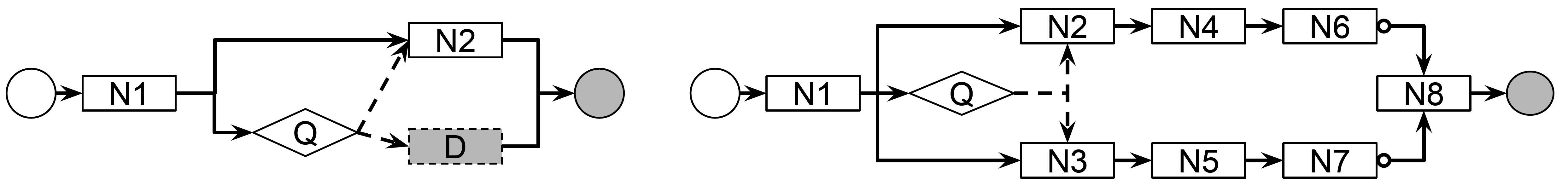
Figure 1: Two D²NN examples. Input and output nodes are drawn as circles with the output nodes shaded. Function nodes are drawn as rectangles (regular nodes) or diamonds (control nodes). Dummy nodes are shaded. Data edges are drawn as solid arrows and control edges as dashed arrows. A data edge with a user defined default value is decorated with a circle.

D²NNs are motivated by the need for computational efficiency, in particular, by the need to deploy deep networks on mobile devices and data centers. Mobile devices are constrained by energy and power, limiting the amount of computation that can be executed. Data centers need energy efficiency to scale to higher throughput and to save operating cost. D²NNs provide a way to improve computational efficiency by selective execution, pruning unnecessary computation depending on input. D²NNs also make it possible to use a bigger network under a computation budget by executing only a subset of the neurons each time.

A D²NN is trained end to end. That is, regular modules and control modules are jointly trained to optimize both accuracy and efficiency. We achieve such training by integrating backpropagation with reinforcement learning, necessitated by the non-differentiability of control modules.

Compared to prior work that optimizes computational efficiency in computer vision and machine learning, our work is distinctive in four aspects: (1) the decisions on selective execution are part of the network inference and are learned end to end together with the rest of the network, as opposed to hand-designed or separately learned [23, 29, 2]; (2) D²NNs allow more flexible network architectures and execution sequences including parallel paths, as opposed to architectures with less variance [12, 27]; (3) our D²NNs directly optimize arbitrary efficiency metric that is defined by the user, while previous work has no such flexibility because they improve efficiency indirectly through sparsity constraints[5, 7, 27]. (4) our method optimizes metrics such as the F-score that does not decompose over individual examples. This is an issue not addressed in prior work. We will elaborate on these differences in the Related Work section of this paper.

We perform extensive experiments to validate our D²NNs algorithms. We evaluate various D²NN architectures on several tasks. They demonstrate that D²NNs are general, flexible, and can effectively improve computational efficiency.

Our main contribution is the D²NN framework that allows a user to augment a static feed-forward network with control modules to achieve dynamic selective execution. We show that D²NNs allow a wide variety of topologies while sharing a unified training algorithm. To our knowledge, D²NN is the first single framework that can support various qualitatively different efficient network designs, including cascade designs and coarse-to-fine designs. Our D²NN framework thus provides a new tool for designing and training computationally efficient neural network models.

2 Related work

Input-dependent execution has been widely used in computer vision, from cascaded detectors [31, 15] to hierarchical classification [10, 6]. The key difference of our work from prior work is that we jointly learn both visual features and control decisions end to end, whereas prior work either hand-designs features and control decisions (e.g. thresholding), or learns them separately.

In the context of deep networks, two lines of prior work have attempted to improve computational efficiency. One line of work tries to eliminate redundancy in data or computation in a way that is input-independent. The methods include pruning networks [18, 32, 3], approximating layers with simpler functions [13, 33], and using number representations of limited precision [8, 17]. The other line of work exploits the fact that not all inputs require the same amount of computation, and explores input-dependent execution of DNNs. Our work belongs to the second line, and we will contrast our work mainly with them. In fact, our input-dependent D²NN can be combined with input-independent methods to achieve even better efficiency.

Among methods leveraging input-dependent execution, some use pre-defined execution-control policies. For example, cascade methods [23, 29] rely on manually-selected thresholds to control execution; Dynamic Capacity Network [2] designs a way to directly calculate a saliency map for execution control. Our D²NNs, instead, are fully learn-able; the execution-control policies of D²NNs do not require manual design and are learned together with the rest of the network.

Our work is closely related to conditional computation methods  [5, 7, 27], which activate part of a network depending on input. They learn policies to encourage sparse neural activations[5] or sparse expert networks[27]. Our work differs from these methods in several ways. First, our control policies are learned to directly optimize arbitrary user-defined global performance metrics, whereas conditional computation methods have only learned policies that encourage sparsity. In addition, D²NNs allow more flexible control topologies. For example, in [5], a neuron (or block of neurons) is the unit controllee of their control policies; in [27], an expert is the unit controllee. Compared to their fixed types of controllees, our control modules can be added in any point of the network and control arbitrary subnetworks. Also, various policy parametrization can be used in the same D²NN framework. We show a variety of parameterizations (as different controller networks) in our D²NN examples, whereas previous conditional computation works have used some fixed formats: For example, control policies are parametrized as the sigmoid or softmax of an affine transformation of neurons or inputs [5, 27].

Our work is also related to attention models [11, 25, 16]. Note that attention models can be categorized as hard attention [25, 4, 2] versus soft [16, 28]. Hard attention models only process the salient parts and discard others (e.g. processing only a subset of image subwindows); in contrast, soft attention models process all parts but up-weight the salient parts. Thus only hard attention models perform input-dependent execution as D²NNs do. However, hard attention models differ from D²NNs because hard attention models have typically involved only one attention module whereas D²NNs can have multiple attention (controller) modules — conventional hard attention models are “single-threaded” whereas D²NN can be “multi-threaded”. In addition, prior work in hard attention models have not directly optimized for accuracy-efficiency trade-offs. It is also worth noting that many mixture-of-experts methods [20, 21, 14] also involve soft attention by soft gating experts: they process all experts but only up-weight useful experts, thus saving no computation.

D²NNs also bear some similarity to Deep Sequential Neural Networks (DSNN) [12] in terms of input-dependent execution. However, it is important to note that although DSNNs’ structures can in principle be used to optimize accuracy-efficiency trade-offs, DSNNs are not for the task of improving efficiency and have no learning method proposed to optimize efficiency. And the method to effectively optimize for efficiency-accuracy trade-off is non-trivial as is shown in the following sections. Also, DSNNs are single-threaded: it always activates exactly one path in the computation graph, whereas for D²NNs it is possible to have multiple paths or even the entire graph activated.

3 Definition and Semantics of D²NNs

Here we precisely define a D²NN and describe its semantics, i.e. how a D²NN performs inference.

D²NN definition A D²NN is defined as a directed acyclic graph (DAG) without duplicated edges. Each node can be one of the three types: input nodes, output nodes, and function nodes. An input or output node represents an input or output of the network (e.g. a vector). A function node represents a (differentiable) function that maps a vector to another vector. Each edge can be one of the two types: data edges and control edges. A data edge represents a vector sent from one node to another, the same as in a conventional DNN. A control edge represents a control signal, a scalar, sent from one node to another. A data edge can optionally have a user-defined “default value”, representing the output that will still be sent even if the function node does not execute.

For simplicity, we have a few restrictions on valid D²NNs: (1) the outgoing edges from a node are either all data edges or all control edges (i.e. cannot be a mix of data edges and control edges); (2) if a node has an incoming control edge, it cannot have an outgoing control edge. Note that these two simplicity constraints do not in any way restrict the expressiveness of a D²NN. For example, to achieve the effect of a node with a mix of outgoing data edges and control edges, we can just feed its data output to a new node with outgoing control edges and let the new node be an identity function.

We call a function node a control node if its outgoing edges are control edges. We call a function node a regular node if its outgoing edges are data edges. Note that it is possible for a function node to take no data input and output a constant value. We call such nodes “dummy” nodes. We will see that the “default values” and “dummy” nodes can significantly extend the flexibility of D²NNs. Hereafter we may also call function nodes “subnetwork”, or “modules” and will use these terms interchangeably. Fig. 1 illustrates simple D²NNs with all kinds of nodes and edges.

D²NN Semantics Given a D²NN, we perform inference by traversing the graph starting from the input nodes. Because a D²NN is a DAG, we can execute each node in a topological order (the parents of a node are ordered before it; we take both data edges and control edges in consideration), same as conventional DNNs except that the control nodes can cause the computation of some nodes to be skipped.

After we execute a control node, it outputs a set of control scores, one for each of its outgoing control edges. The control edge with the highest score is “activated”, meaning that the node being controlled is allowed to execute. The rest of the control edges are not activated, and their controllees are not allowed to execute. For example, in Fig 1 (right), the node Q controls N2 and N3. Either N2 or N3 will execute depending on which has the higher control score.

Although the main idea of the inference (skipping nodes) seems simple, due to D²NNs’ flexibility, the inference topology can be far more complicated. For example, in the case of a node with multiple incoming control edges (i.e. controlled by multiple controllers), it should execute if any of the control edges are activated. Also, when the execution of a node is skipped, its output will be either the default value or null. If the output is the default value, subsequent execution will continue as usual. If the output is null, any downstream nodes that depend on this output will in turn skip execution and have a null output unless a default value has been set. This “null” effect will propagate to the rest of the graph. Fig. 1 (right) shows a slightly more complicated example with default values: if N2 skips execution and outputs null, so will N4 and N6. But N8 will execute regardless because its input data edge has a default value. In our Experiments Section, we will demonstrate more sophisticated D²NNs.

We can summarize the semantics of D²NNs as follows: a D²NN executes the same way as a conventional DNN except that there are control edges that can cause some nodes to be skipped. A control edge is active if and only if it has the highest score among all outgoing control edges from a node. A node is skipped if it has incoming control edges and none of them is active, or if one of its inputs is null. If a node is skipped, its output will be either null or a user-defined default value. A null will cause downstream nodes to be skipped whereas a default value will not.

A D²NN can also be thought of as a program with conditional statements. Each data edge is equivalent to a variable that is initialized to either a default value or null. Executing a function node is equivalent to executing a command assigning the output of the function to the variable. A control edge is equivalent to a boolean variable initialized to False. A control node is equivalent to a “switch-case” statement that computes a score for each of the boolean variables and sets the one with the largest score to True. Checking the conditions to determine whether to execute a function is equivalent to enclosing the function with an “if-then” statement. A conventional DNN is a program with only function calls and variable assignments without any conditional statements, whereas a D²NN introduces conditional statements with the conditions themselves generated by learnable functions.

4 D²NN Learning

Due to the control nodes, a D²NN cannot be trained the same way as a conventional DNN. The output of the network cannot be expressed as a differentiable function of all trainable parameters, especially those in the control nodes. As a result, backpropagation cannot be directly applied. The main difficulty lies in the control nodes, whose outputs are discretized into control decisions. This is similar to the situation with hard attention models [25, 4], which use reinforcement learning. Here we adopt the same general strategy.

Learning a Single Control Node For simplicity of exposition we start with a special case where there is only one control node. We further assume that all parameters except those of this control node have been learned and fixed. That is, the goal is to learn the parameters of the control node to maximize a user-defined reward, which in our case is a combination of accuracy and efficiency. This results in a classical reinforcement learning setting: learning a control policy to take actions so as to maximize reward. We base our learning method on Q-learning [26, 30]. We let each outgoing control edge represent an action, and let the control node approximate the action-value (Q) function, which is the expected return of an action given the current state (the input to the control node).

It is worth noting that unlike many prior works that use deep reinforcement learning, a D²NN is not recurrent. For each input to the network (e.g. an image), each control node only executes once. And the decisions of a control node completely depend on the current input. As a result, an action taken on one input has no effect on another input. That is, our reinforcement learning task consists of only one time step. Our one time-step reinforcement learning task can also be seen as a contextual bandit problem, where the context vector is the input to the control module, and the arms are the possible action outputs of the module. The one time-step setting simplifies our Q-learning objective to that of the following regression task:

$$L=(Q(\boldsymbol{s},\boldsymbol{a})-r)^{2},$$ (1)

where $r$ is a user-defined reward, $\boldsymbol{a}$ is an action, $\boldsymbol{s}$ is the input to control node, and $Q$ is computed by the control node. As we can see, training a control node here is the same as training a network to predict the reward for each action under an L2 loss. We use mini-batch gradient descent; for each training example in a mini-batch, we pick the action with the largest $Q$, execute the rest of the network, observe a reward, and perform backpropagation using the L2 loss in Eqn. 1.

During training we also perform $\epsilon$-greedy exploration — instead of always choosing the action with the best $Q$ value, we choose a random action with probability $\epsilon$. The hyper-parameter $\epsilon$ is initialized to $1$ and decreases over time. The reward $r$ is user defined. Since our goal is to optimize the trade-off between accuracy and efficiency, in our experiments we define the reward as a combination of an accuracy metric $A$ (for example, F-score) and an efficiency metric $E$ (for example, the inverse of the number of multiplications), that is, $\lambda A+(1-\lambda)E$ where $\lambda$ balances the trade-off.

Mini-Bags for Set-Based Metrics Our training algorithm so far has defined the state as a single training example, i.e., the control node takes actions and observes rewards on each training example independent of others. This setup, however, introduces a difficulty for optimizing for accuracy metrics that cannot be decomposed over individual examples.

Consider precision in the context of binary classification. Given predictions on a set of examples and the ground truth, precision is defined as the proportion of true positives among the predicted positives. Although precision can be defined on a single example, precision on a set of examples does not generally equal the average of the precisions of individual examples. In other words, precision as a metric does not decompose over individual examples and can only be computed using a set of examples jointly. This is different from decomposable metrics such as error rate, which can be computed as the average of the error rates of individual examples. If we use precision as our accuracy metric, it is not clear how to define a reward independently for each example such that maximizing this reward independently for each example would optimize the overall precision. In general, for many metrics, including precision and F-score, we cannot compute them on individual examples and average the results. Instead, we must compute them using a set of examples as a whole. We call such metrics “set-based metrics”. Our learning setup so far is ill-equipped for such metrics because a reward is defined on each example independently.

To address this issue we generalize the definition of a state from a single input to a set of inputs. We define such a set of inputs as a mini-bag. With a mini-bag of images, any set-based metric can be computed and can be used to directly define a reward. Note that a mini-bag is different from a mini-batch which is commonly used for batch updates in gradient decent methods. Actually in our training, we calculate gradients using a mini-batch of mini-bags. Now, an action on a mini-bag $\mathbf{s}=(s_{1},\ldots,s_{m})$ is now a joint action $\mathbf{a}=(a_{1},\ldots,a_{m})$ consisting of individual actions $a_{i}$ on example $s_{i}$. Let $\mathbf{Q}(\mathbf{s},\mathbf{a})$ be the joint action-value function on the mini-bag $\mathbf{s}$ and the joint action $\mathbf{a}$. We constrain the parametric form of $\mathbf{Q}$ to decompose over individual examples:

$$\mathbf{Q}=\sum_{i=1}^{m}Q(s_{i},a_{i}),$$ (2)

where $Q(s_{i},a_{i})$ is a score given by the control node when choosing the action $a_{i}$ for example $s_{i}$. We then define our new learning objective on a mini-bag of size $m$ as

$$L=(r-\mathbf{Q}(\mathbf{s},\mathbf{a}))^{2}=(r-\sum_{i=1}^{m}Q(s_{i},a_{i}))^{2},$$ (3)

where $r$ is the reward observed by choosing the joint action $\mathbf{a}$ on mini-bag $\mathbf{s}$. That is, the control node predicts an action-value for each example such that their sum approximates the reward defined on the whole mini-bag.

It is worth noting that the decomposition of $\mathbf{Q}$ into sums (Eqn. 2) enjoys a nice property: the best joint action $\mathbf{a}^{*}$ under the joint action-value $\mathbf{Q}(\mathbf{s},\mathbf{a})$ is simply the concatenation of the best actions for individual examples because maximizing

$$\mathbf{a}^{*}=\arg\max_{\mathbf{a}}(\mathbf{Q}(\mathbf{s},\mathbf{a}))=\arg\max_{\mathbf{a}}({\sum_{i=1}^{m}Q(s_{i},a_{i})})$$ (4)

is equivalent to maximizing the individual summands:

$$a_{i}^{*}=\arg\max_{a_{i}}Q(s_{i},a_{i}),i=1,2...m.$$ (5)

That is, during test time we still perform inference on each example independently.

Another implication of the mini-bag formulation is:

$$\frac{\partial L}{\partial x_{i}}=2(r-\sum_{j=1}^{m}Q(s_{j},a_{j}))\frac{\partial Q(s_{i},a_{i})}{\partial x_{i}},$$ (6)

where $x_{i}$ is the output of any internal neuron for example $i$ in the mini-bag. This shows that there is no change to the implementation of backpropagation except that we scale the gradient using the difference between the mini-bag Q-value $\mathbf{Q}$ and reward $r$.

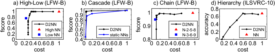
Figure 2: The accuracy-cost or fscore-cost curves of various D²NN architectures, as well as conventional DNN baselines consisting of only regular nodes.

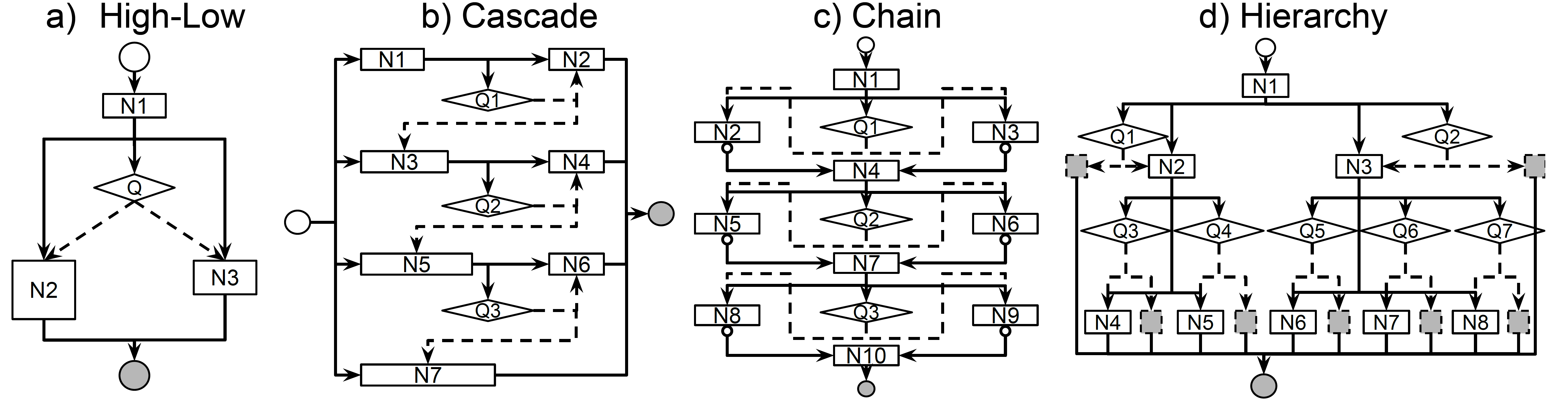
Figure 3: Four different D²NN architectures.

Joint Training of All Nodes We have described how to train a single control node. We now describe how to extend this strategy to all nodes including additional control nodes as well as regular nodes. If a D²NN has multiple control nodes, we simply train them together. For each mini-bag, we perform backpropagation for multiple losses together. Specifically, we perform inference using the current parameters, observe a reward for the whole network, and then use the same reward (which is a result of the actions of all control nodes) to backpropagate for each control node.

For regular nodes, we can place losses on them the same as on conventional DNNs. And we perform backpropagation on these losses together with the control nodes. The implementation of backpropagation is the same as conventional DNNs except that each training example have a different network topology (execution sequence). And if a node is skipped for a particular training example, then the node does not have a gradient from the example.

It is worth noting that our D²NN framework allows arbitrary losses to be used for regular nodes. For example, for classification we can use the cross-entropy loss on a regular node. One important detail is that the losses on regular nodes need to be properly weighted against the losses on the control nodes; otherwise the regular losses may dominate, rendering the control nodes ineffective. One way to eliminate this issue is to use Q-learning losses on regular nodes as well, i.e. treating the outputs of a regular node as action-values. For example, instead of using the cross-entropy loss on the classification scores, we treat the classification scores as action-values—an estimated reward of each classification decision. This way Q-learning is applied to all nodes in a unified way and no additional hyperparameters are needed to balance different kinds of losses. In our experiments unless otherwise noted we adopt this unified approach.

5 Experiments

We here demonstrate four D²NN structures motivated by different demands of efficient network design to show its flexibility and effectiveness, and compare D²NNs’ ability to optimize efficiency-accuracy trade-offs with prior work.

We implement the D²NN framework in Torch. Torch provides functions to specify the subnetwork architecture inside a function node. Our framework handles the high-level communication and loss propagation.

High-Low Capacity D²NN Our first experiment is with a simple D²NN architecture that we call “high-low capacity D²NN”. It is motivated by that we can save computation by choosing a low-capacity subnetwork for easy examples. It consists of a single control nodes (Q) and three regular nodes (N1-N3) as in Fig. 3a). The control node Q chooses between a high-capacity N2 and a low-capacity N3; the N3 has fewer neurons and uses less computation. The control node itself has orders of magnitude fewer computation than regular nodes (this is true for all D²NNs demonstrated).

We test this hypothesis using a binary classification task in which the network classifies an input image as face or non-face. We use the Labeled Faces in the Wild [19, 22] dataset. Specifically, we use the 13k ground truth face crops (112$\times$112 pixels) as positive examples and randomly sampled 130k background crops (with an intersection over union less than 0.3) as negative examples. We hold out 11k images for validation and 22k for testing. We refer to this dataset as LFW-B and use it as a testbed to validate the effectiveness of our new D²NN framework.

To evaluate performace we measure accuracy using the F1 score, a better metric than percentage of correct predictions for an unbalanced dataset. We measure computational cost using the number of multiplications following prior work [2, 27] and for reproductivity. Specifically, we use the number of multiplications (control nodes included), normalized by a conventional DNN consisting of N1 and N2, that is, the high-capacity execution path. Note that our D²NNs also allow to use other efficiency measurement such as run-time, latency.

During training we define the Q-learning reward as a linear combination of accuracy $A$ and efficiency $E$ (negative cost): $r=\lambda A+(1-\lambda)E$ where $\lambda\in[0,1]$. We train instances of high-low capacity D²NNs using different $\lambda$’s. As $\lambda$ increases, the learned D²NN trades off efficiency for accuracy. Fig. 2a) plots the accuracy-cost curve on the test set; it also plots the accuracy and efficiency achieved by a conventional DNN with only the high capacity path N1+N2 (High NN) and a conventional DNN with only the low capacity path N1+N3 (Low NN).

As we can see, the D²NN achieves a trade-off curve close to the upperbound: there are points on the curve that are as fast as the low-capacity node and as accurate as the high-capacity node. Fig. 4(left) plots the distribution of examples going through different execution paths. It shows that as $\lambda$ increases, accuracy becomes more important and more examples go through the high-capacity node. These results suggest that our learning algorithm is effective for networks with a single control node.

With inference efficiency improved, we also observe that for training, a D²NN typically takes 2-4 times more iterations to converge than a DNN, depending on particular model capacities, configurations and trade-offs.

Cascade D²NN We next experiment with a more sophisticated design that we call a “cascade D²NN” (Fig. 3b). It is inspired by the standard cascade design commonly used in computer vision. The intuition is that many negative examples may be rejected early using simple features. The cascade D²NN consists of seven regular nodes (N1-N7) and three control nodes (Q1-Q3). N1-N7 form 4 cascade stages (i.e. 4 conventional DNNs, from small to large) of the cascade: N1+N2, N3+N4, N5+N6, N7. Each control node decides whether to execute the next cascade stage or not.

We evaluate the network on the same LFW-B face classification task using the same evaluation protocol as in the high-low capacity D²NN. Fig. 2b) plots the accuracy-cost tradeoff curve for the D²NN. Also included are the accuracy-cost curve (“static NNs”) achieved by the four conventional DNNs as baselines, each trained with a cross-entropy loss. We can see that the cascade D²NN can achieve a close to optimal trade-off, reducing computation significantly with negligible loss of accuracy. In addition, we can see that our D²NN curve outperforms the trade-off curve achieved by varying the design and capacity of static conventional networks. This result demonstrates that our algorithm is successful for jointly training multiple control nodes.

For a cascade, wall time of inference is often an important consideration. Thus we also measure the inference wall time (excluding data loading with 5 runs) in this Cascade D²NN. We find that a 82% wall-time cost corresponds to a 53% number-of-multiplication cost; and a 95% corresponds to a 70%. Defining reward directly using wall time can further reduce the gap.

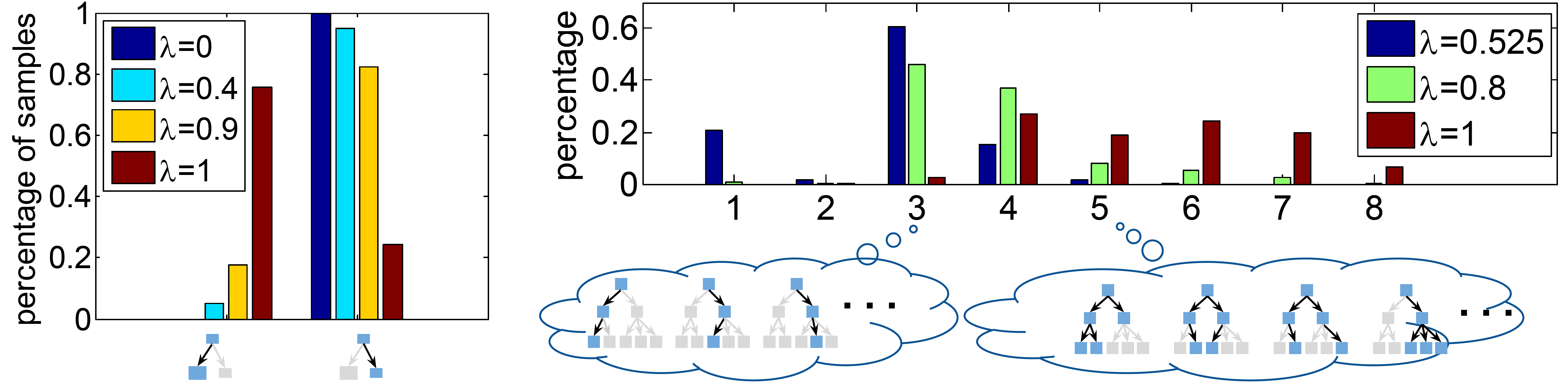
Figure 4: Distribution of examples going through different execution paths. Skipped nodes are in grey. The hyperparameter $\lambda$ controls the trade-off between accuracy and efficiency. A bigger $\lambda$ values accuracy more. Left: for the high-low capacity D²NN. Right: for the hierarchical D²NN. The X-axis is the number of nodes activated.

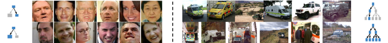
Figure 5: Examples with different paths in a high-low D²NN (left) and a hierarchical D²NN (right).

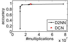
Figure 6: Accuracy-cost curve for a chain D²NN on the CMNIST task compared to DCN [2].

Chain D²NN Our third design is a “Chain D²NN” (Fig. 3c). The network is shaped as a chain, where each link consists of a control node selecting between two (or more) regular nodes. In other words, we perform a sequence of vector-to-vector transforms; for each transform we choose between several subnetworks. One scenario that we can use this D²NN is that the configuration of a conventional DNN (e.g. number of layers, filter sizes) cannot be fully decided. Also, it can simulate shortcuts between any two layers by using an identity function as one of the transforms. This chain D²NN is qualitatively different from other D²NNs with a tree-shaped data graph because it allows two divergent data paths to merge again. That is, the number of possible execution paths can be exponential to the number of nodes.

In Fig. 3c), the first link is that Q1 chooses between a low-capacity N2 and a high-capacity N3. If one of them is chosen, the other will output a default value zero. The node N4 adds the outputs of N2 and N3 together. Fig. 2c) plots the accuracy-cost curve on the LFW-B task. The two baselines are: a conventional DNN with the lowest capacity path (N1-N2-N5-N8-N10), and a conventional DNN with the highest capacity path (N1-N3-N6-N9-N10). The cost is measured as the number of multiplications, normalized by the cost of the high-capacity baseline.

Fig. 2c) shows that the chain D²NN achieves a trade-off curve close to optimal and can speed up computation significantly with little accuracy loss. This shows that our learning algorithm is effective for a D²NN whose data graph is a general DAG instead of a tree.

Hierarchical D²NN In this experiment we design a D²NN for hierarchical multiclass classification. The idea is to first classify images to coarse categories and then to fine categories. This idea has been explored by numerous prior works [24, 6, 10], but here we show that the same idea can be implemented via a D²NN trained end to end.

We use ILSVRC-10, a subset of the ILSVRC-65 [9]. In ILSVRC-10, 10 classes are organized into a 3-layer hierarchy: 2 superclasses, 5 coarse classes and 10 leaf classes. Each class has 500 training images, 50 validation images, and 150 test images. As in Fig. 3d), the hierarchy in this D²NN mirrors the semantic hierarchy in ILSVRC-10. An image first goes through the root N1. Then Q1 decides whether to descend the left branch (N2 and its children), and Q2 decides whether to descend the right branch (N3 and its children). The leaf nodes N4-N8 are each responsible for classifying two fine-grained leaf classes. It is important to note that an input image can go down parallel paths in the hierarchy, e.g. descending both the left branch and the right branch, because Q1 and Q2 make separate decisions. This “multi-threading” allows the network to avoid committing to a single path prematurely if an input image is ambiguous.

Fig. 2d) plots the accuracy-cost curve of our hierarchical D²NN. The accuracy is measured as the proportion of correctly classified test examples. The cost is measured as the number of multiplications, normalized by the cost of a conventional DNN consisting only of the regular nodes (denoted as NN in the figure). We can see that the hierarchical D²NN can match the accuracy of the full network with about half of the computational cost.

Fig. 4(right) plots for the hierarchical D²NN the distribution of examples going through execution sequences with different numbers of nodes activated. Due to the parallelism of D²NN, there can be many different execution sequences. We also see that as $\lambda$ increases, accuracy is given more weight and more nodes are activated.

Comparison with Dynamic Capacity Networks In this experiment we empirically compare our approach to closely related prior work. Here we compare D²NNs with Dynamic Capacity Networks (DCN) [2], for which efficency measurement is the absolute number of multiplications. Given an image, a DCN applies an additional high capacity subnetwork to a set of image patches, selected using a hand-designed saliency based policy. The idea is that more intensive processing is only necessary for certain image regions.

To compare, we evaluate with the same multiclass classification task on the Cluttered MNIST [25], which consists of MNIST digits randomly placed on a background cluttered with fragments of other digits. We train a chain D²NN of length 4 , which implements the same idea of choosing a high-capacity alternative subnetwork for certain inputs. Fig. 6 plots the accuracy-cost curve of our D²NN as well as the accuracy-cost point achieved by the DCN in  [2]—an accuracy of $0.9861$ and and a cost of $2.77\times 10^{7}$. The closest point on our curve is an slightly lower accuracy of $0.9698$ but slightly better efficiency (a cost of $2.66\times 10^{7}$). Note that although our accuracy of $0.9698$ is lower, it compares favorably to those of other state-of-the-art methods such as DRAW [16]: $0.9664$ and RAM [25]: $0.9189$.

Visualization of Examples in Different Paths In Fig. 5 (left), we show face examples in the high-low D²NN for $\lambda$=0.4. Examples in low-capacity path are generally easier (e.g. more frontal) than examples in high-capacity path. In Fig. 5 (right), we show car examples in the hierarchical D²NN with 1) a single path executed and 2) the full graph executed (for $\lambda$=1). They match our intuition that examples with a single path executed should be easier (e.g. less occlusion) to classify than examples with the full graph executed.

CIFAR-10 Results We train a Cascade D²NN on CIFAR-10 where the corresponded DNN baseline is the ResNet-110. We initialize this D²NN with pre-trained ResNet-110 weights, apply cross-entropy losses on regular nodes, and tune the mixed-loss weight as explained in Sec. 4. We see a 30% reduction of cost with a 2% loss (relative) on accuracy, and a 62% reduction of cost with a 7% loss (relative) on accuracy. The D²NN’s ability to improve efficiency relies on the assumption that not all inputs require the same amount of computation. In CIFAR-10, all images are low resolution (32 $\times$ 32), and it is likely that few images are significantly easier to classify than others. As a result, the efficiency improvement is modest compared to other datasets.

6 Conclusion

We have introduced Dynamic Deep Neural Networks (D²NN), a new type of feed-forward deep neural networks that allow selective execution. Extensive experiments have demonstrated that D²NNs are flexible and effective for optimizing accuracy-efficiency trade-offs.

7 Acknowledgments

This work is partially supported by the National Science Foundation under Grant No. 1539011 and gifts from Intel.

Appendix

Appendix A A Implementation Details

We implement the D²NN framework in Torch [1]. Torch already provides implementations of conventional neural network modules (nodes). So a user can specify the subnetwork architecture inside a control node or a regular node using existing Torch functionalities. Our framework then handles the communication between the user-defined nodes in the forward and backward pass.

To handle parallel paths, default-valued nodes and nodes with multiple data parents, we need to keep track of an example’s execution status (which nodes are activated by this example) and output status (which nodes have output for this example). An example’s output status is different from its execution status if some nodes are not activated but have default values. For runtime efficiency, we implement the tracking of examples at the mini-batch level. That is, we perform forward and backward passes for a mini-batch of examples as a regular DNN does. Each mini-batch consists of several mini-bags of images.

We describe the implementation of D²NN learning procedure as two steps. First, the preprocessing step: When a user-defined D²NN model is fed into our framework, we first perform a breadth-first search to get the DAG orders of nodes while performing structure error checks, contructing data and control relationships between nodes and calculating the cost (number of multiplications) of each node.

After the preprocessing, the training step is similar to a regular DNN: a forward pass and a backward pass. All nodes are visited according to a topological ordering in a forward pass and the reverse ordering in a backward pass.

For each function node, the forward pass has three steps: fetch inputs, forward inside the node, and send data or control signals to children nodes. When dealing with multiple data inputs and multiple control signals, the D²NN will filter examples with more than one null inputs or all negative control signals. When a default value has been set for a node, all examples have to send out data. If the node is not activated for a particular example, the output will take the default value. A backward pass has similar logic: fetch gradients from children, perform the backward pass inside and send out gradients to parents. It is worth noting that when a default value is used in a node, the gradients can be blocked by this node because it is not actually executed.

Appendix B B ILSVRC-10 Semantic Hierarchy

The ILSVRC-10 dataset is a subset of the ILSVRC-65 dataset [9]. In our ILSVRC-10, there are 10 classes organized into a 3-layer hierarchy: 2 superclasses, 5 coarse classes and 10 leaf classes as in Fig 7. Each class has 500 training images, 50 validation images, and 150 test images.

Figure 7: The semantic class hierarchy of the ILSVRC-10 dataset.

Appendix C C Configurations

High-Low Capacity D²NN The high-low capacity D²NN consists of a single control node (Q) and three regular nodes (N1,N2,N3) as illustrated in Fig. 3a).

• Node N1: a convolutional layer with a 3$\times$3 filter size, 8 filters and a stride of 2, followed by a 3$\times$3 max-pooling layer with a stride of 2.

• Node N2: a convolutional layer with a 3$\times$3 filter size and 16 filters, followed by a 3$\times$3 max-pooling layer with a stride of 2. The output is reshaped and fed into a fully connected layer with 512 neurons followed by another fully connected layer with the 2-class output.

• Node N3: three 3$\times$3 max-pooling layers, each with a stride of 2, followed by two fully connected layers with 32 neurons and the 2-class output.

• Node Q1: a convolutional layer with a 3$\times$3 filter size and 2 filters, followed by a 3$\times$3 max-pooling layer with a stride of 2. The output is reshaped and fed into a fully connected layer with 128 neurons followed by another fully connected layer with the 2-action output.

Cascade D²NN The cascade D²NN consists of a sequence of four regular nodes (N1 to N7) and three control nodes (Q1-Q3) as in Fig. 3b).

• Node N1: a convolutional layer with a 3$\times$3 filter size, 2 filters and a stride of 2, followed by a 3$\times$3 max-pooling layer with a stride of 2.

• Node N2: three 3$\times$3 max-pooling layers with strides of 2. The output is reshaped and fed into a fully connected layer with the 2-class output.

• Node N3: two convolutional layers with both 3$\times$3 filter sizes and 2, 8 filters respectively, each followed by a 3$\times$3 max-pooling layer with a stride of 2.

• Node N4: two 3$\times$3 max-pooling layers with strides of 2. The output is reshaped and fed into a fully connected layer with the 2-class output.

• Node N5: two convolutional layers with both 3$\times$3 filter sizes and 4, 16 filters respectively, each followed by a 3$\times$3 max-pooling layer with a stride of 2.

• Node N6: two 3$\times$3 max-pooling layers with strides of 2. The output is reshaped and fed into a fully connected layer with the 2-class output.

• Node N7: five convolutional layers with all 3$\times$3 filter sizes and 2, 8, 32, 32, 64 filters repectively, each followed by a 3$\times$3 max-pooling layer with a stride of 2 except for the third and fifth layer. The output is reshaped and fed into a fully connected layer with 512 neurons followed by another fully connected layer with the 2-class output.

• Node Q1, Q2, Q3: the input is reshaped and fed into a fully connected layer with the 2-action output.

Chain D²NN The Chain D²NN is shaped as a chain, where each link consists of a control node selecting between two regular nodes. In the experiments of LFW-B dataset, we use a 3-stage Chain D²NN as in Fig. 3c).

• Node N1: a convolutional layer with a 3$\times$3 filter size, 2 filters and a stride of 2, followed by a 3$\times$3 max-pooling layer with a stride of 2.

• Node N2: a convolutional layer with a 1$\times$1 filter size and 16 filters.

• Node N3: a convolutional layer with a 3$\times$3 filter size and 16 filters.

• Node N4: a 3$\times$3 max-pooling layer with a stride of 2.

• Node N5: a convolutional layer with a 1$\times$1 filter size and 32 filters.

• Node N6: two convolutional layers with both 3$\times$3 filter sizes and 32, 32 filters repectively.

• Node N7: a 3$\times$3 max-pooling layer with a stride of 2.

• Node N8: a convolutional layer with a 1$\times$1 filter size and 32 filters followed by a 3$\times$3 max-pooling layer with a stride of 2. The output is reshaped and fed into a fully connected layer with 256 neurons.

• Node N9: a convolutional layer with a 3$\times$3 filter size and 64 filters. The output is reshaped and fed into a fully connected layer with 256 neurons.

• Node N10: a fully connected layer with the 2-class output.

• Node Q1: a convolutional layer with a 3$\times$3 filter size and 8 filters with a 3$\times$3 max-pooling layer with a stride of 2 before and a 3$\times$3 max-pooling layer with a stride of 2 after. The output is reshaped and fed into two fully connected layers with 64 neurons and the 2-action output respectively.

• Node Q2: a 3$\times$3 max-pooling layer with a stride of 2 followed by a convolutional layer with a 3$\times$3 filter size and 4 filters. The output is reshaped and fed into two fully connected layers with 64 neurons and the 2-action output respectively.

• Node Q3: a convolutional layer with a 3$\times$3 filter size and 2 filters. The output is reshaped and fed into two fully connected layers with 64 neurons and the 2-action output respectively.

Hierarchical D²NN Fig. 3d) illustrates the design of our hierarchical D²NN.

• Node N1: a convolutional layer with a 11$\times$11 filter size, 64 filters, a stride of 4 and a 2$\times$2 padding, followed by a 3$\times$3 max-pooling layer with a stride of 2.

• Node N2 and N3: a convolutional layer with a 5$\times$5 filter size, 96 filters and a 2$\times$2 padding.

• Node N4 N8: a 3$\times$3 max-pooling layer with a stride of 2 followed by three convolutional layers with 3$\times$3 filter sizes and 160, 128, 128 filters respectively. The output is fed into a 3$\times$3 max-pooling layer with a stride of 2 and three fully connected layers with 2048 neurons, 2048 neurons and the 2 fine-class output respectively.

• Node Q1 and Q2: two convolutional layers with 5$\times$5, 3$\times$3 filter sizes and 16, 32 filters respectively (the former has a 2$\times$2 padding), each followed by a 3$\times$3 max-pooling layer with a stride of 2. The output is reshaped and fed into three fully connected layers with 1024 neurons, 1024 neurons and the 2-action output respectively.

• Node Q3 Q7: two convolutional layers with 5$\times$5, 3$\times$3 filter sizes and 16, 32 filters respectively (the former has a 2$\times$2 padding), each followed by a 3$\times$3 max-pooling layer with a stride of 2. The output is reshaped and fed into three fully connected layers with 1024 neurons, 1024 neurons and the 2-action output respectively.

Comparison with Dynamic Capacity Networks We train a chain D²NN of length 4 similar to Fig. 3c).

• Node N1: a convolutional layer with a 3$\times$3 filter size and 24 filters.

• Node N3: a convolutional layer with a 3$\times$3 filter size and 24 filters.

• Node N4: a 2$\times$2 max-pooling layer with a stride of 2.

• Node N6: a convolutional layer with a 3$\times$3 filter size and 24 filters.

• Node N7: an identity layer which directly uses inputs as outputs.

• Node N9: a convolutional layer with a 3$\times$3 filter size and 24 filters.

• Node N10: a 2$\times$2 max-pooling layer with a stride of 2.

• Node N12: a convolutional layer with a 3$\times$3 filter size and 24 filters.

• Node N2, N5, N8, N11: an identity layer.

• Node N13: a convolutional layer with a 4$\times$4 filter size, 96 filters, a stride of 2 and no padding, followed by a 11$\times$11 max-pooling layer. The output is reshaped and fed into a fully connected layer with the 10-class output.

• Node Q1: a convolutional layer with a 3$\times$3 filter size and 8 filters with two 2$\times$2 max-pooling layers with strides of 2 before and one 2$\times$2 max-pooling layer with a stride of 2 after. The output is reshaped and fed into two fully connected layers with 256 neurons and the 2-action output respectively.

• Node Q2: a convolutional layer with a 3$\times$3 filter size and 8 filters with a 2$\times$2 max-pooling layer with a stride of 2 before and a 2$\times$2 max-pooling layer with a stride of 2 after. The output is reshaped and fed into two fully connected layers with 256 neurons and the 2-action output respectively.

• Node Q3: a convolutional layer with a 3$\times$3 filter size and 8 filters with a 2$\times$2 max-pooling layer with a stride of 2 before and a 2$\times$2 max-pooling layer with a stride of 2 after. The output is reshaped and fed into two fully connected layers with 256 neurons and the 2-action output respectively.

• Node Q4: a convolutional layer with a 3$\times$3 filter size and 8 filters, followed by a 2$\times$2 max-pooling layer with a stride of 2. The output is reshaped and fed into two fully connected layers with 256 neurons and the 2-action output respectively.

For all 5 D²NNs, all convolutional layers use 1$\times$1 padding and each is followed by a ReLU layer unless specified individually. Each fully connected layer except the output layers is followed by a ReLU layer.

References

- [1] Torch. http://torch.ch/.
- [2] A. Almahairi, N. Ballas, T. Cooijmans, Y. Zheng, H. Larochelle, and A. C. Courville. Dynamic capacity networks. In Proceedings of the 33nd International Conference on Machine Learning, ICML 2016, New York City, NY, USA, June 19-24, 2016, pages 2549–2558, 2016.
- [3] J. M. Alvarez and M. Salzmann. Learning the number of neurons in deep networks. In Advances in Neural Information Processing Systems, pages 2270–2278, 2016.
- [4] J. Ba, V. Mnih, and K. Kavukcuoglu. Multiple object recognition with visual attention. arXiv preprint arXiv:1412.7755, 2014.
- [5] E. Bengio, P.-L. Bacon, J. Pineau, and D. Precup. Conditional computation in neural networks for faster models. arXiv preprint arXiv:1511.06297, 2015.
- [6] S. Bengio, J. Weston, and D. Grangier. Label embedding trees for large multi-class tasks. In Advances in Neural Information Processing Systems, pages 163–171, 2010.
- [7] Y. Bengio, N. Léonard, and A. Courville. Estimating or propagating gradients through stochastic neurons for conditional computation. arXiv preprint arXiv:1308.3432, 2013.
- [8] Y. Chen, T. Luo, S. Liu, S. Zhang, L. He, J. Wang, L. Li, T. Chen, Z. Xu, N. Sun, et al. Dadiannao: A machine-learning supercomputer. In Microarchitecture (MICRO), 2014 47th Annual IEEE/ACM International Symposium on, pages 609–622. IEEE, 2014.
- [9] J. Deng, J. Krause, A. C. Berg, and L. Fei-Fei. Hedging your bets: Optimizing accuracy-specificity trade-offs in large scale visual recognition. In Computer Vision and Pattern Recognition (CVPR), 2012 IEEE Conference on, pages 3450–3457. IEEE, 2012.
- [10] J. Deng, S. Satheesh, A. C. Berg, and F. Li. Fast and balanced: Efficient label tree learning for large scale object recognition. In Advances in Neural Information Processing Systems, pages 567–575, 2011.
- [11] M. Denil, L. Bazzani, H. Larochelle, and N. de Freitas. Learning where to attend with deep architectures for image tracking. Neural computation, 24(8):2151–2184, 2012.
- [12] L. Denoyer and P. Gallinari. Deep sequential neural network. arXiv preprint arXiv:1410.0510, 2014.
- [13] E. L. Denton, W. Zaremba, J. Bruna, Y. LeCun, and R. Fergus. Exploiting linear structure within convolutional networks for efficient evaluation. In Advances in Neural Information Processing Systems, pages 1269–1277, 2014.
- [14] D. Eigen, M. Ranzato, and I. Sutskever. Learning factored representations in a deep mixture of experts. arXiv preprint arXiv:1312.4314, 2013.
- [15] P. F. Felzenszwalb, R. B. Girshick, and D. McAllester. Cascade object detection with deformable part models. In Computer vision and pattern recognition (CVPR), 2010 IEEE conference on, pages 2241–2248. IEEE, 2010.
- [16] K. Gregor, I. Danihelka, A. Graves, D. J. Rezende, and D. Wierstra. Draw: A recurrent neural network for image generation. In Proceedings of the 32nd International Conference on Machine Learning (ICML-15). Springer, JMLR Workshop and Conference Proceedings, 2015.
- [17] S. Gupta, A. Agrawal, K. Gopalakrishnan, and P. Narayanan. Deep learning with limited numerical precision. In Proceedings of the 32nd International Conference on Machine Learning (ICML-15), pages 1737–1746, 2015.
- [18] S. Han, J. Pool, J. Tran, and W. Dally. Learning both weights and connections for efficient neural network. In Advances in Neural Information Processing Systems, pages 1135–1143, 2015.
- [19] G. B. Huang, M. Ramesh, T. Berg, and E. Learned-Miller. Labeled faces in the wild: A database for studying face recognition in unconstrained environments. Technical Report 07-49, University of Massachusetts, Amherst, October 2007.
- [20] R. A. Jacobs, M. I. Jordan, S. J. Nowlan, and G. E. Hinton. Adaptive mixtures of local experts. Neural computation, 3(1):79–87, 1991.
- [21] M. I. Jordan and R. A. Jacobs. Hierarchical mixtures of experts and the em algorithm. Neural computation, 6(2):181–214, 1994.
- [22] G. B. H. E. Learned-Miller. Labeled faces in the wild: Updates and new reporting procedures. Technical Report UM-CS-2014-003, University of Massachusetts, Amherst, May 2014.
- [23] H. Li, Z. Lin, X. Shen, J. Brandt, and G. Hua. A convolutional neural network cascade for face detection. In Proceedings of the IEEE Conference on Computer Vision and Pattern Recognition, pages 5325–5334, 2015.
- [24] B. Liu, F. Sadeghi, M. Tappen, O. Shamir, and C. Liu. Probabilistic label trees for efficient large scale image classification. In Proceedings of the IEEE Conference on Computer Vision and Pattern Recognition, pages 843–850, 2013.
- [25] V. Mnih, N. Heess, A. Graves, et al. Recurrent models of visual attention. In Advances in Neural Information Processing Systems, pages 2204–2212, 2014.
- [26] V. Mnih, K. Kavukcuoglu, D. Silver, A. Graves, I. Antonoglou, D. Wierstra, and M. Riedmiller. Playing atari with deep reinforcement learning. arXiv preprint arXiv:1312.5602, 2013.
- [27] N. Shazeer, A. Mirhoseini, K. Maziarz, A. Davis, Q. Le, G. Hinton, and J. Dean. Outrageously large neural networks: The sparsely-gated mixture-of-experts layer. arXiv preprint arXiv:1701.06538, 2017.
- [28] M. F. Stollenga, J. Masci, F. Gomez, and J. Schmidhuber. Deep networks with internal selective attention through feedback connections. In Advances in Neural Information Processing Systems, pages 3545–3553, 2014.
- [29] Y. Sun, X. Wang, and X. Tang. Deep convolutional network cascade for facial point detection. In Computer Vision and Pattern Recognition (CVPR), 2013 IEEE Conference on, pages 3476–3483. IEEE, 2013.
- [30] R. S. Sutton and A. G. Barto. Reinforcement learning: An introduction, volume 1.
- [31] P. Viola and M. J. Jones. Robust real-time face detection. International journal of computer vision, 57(2):137–154, 2004.
- [32] W. Wen, C. Wu, Y. Wang, Y. Chen, and H. Li. Learning structured sparsity in deep neural networks. In Advances in Neural Information Processing Systems, pages 2074–2082, 2016.
- [33] X. Zhang, J. Zou, K. He, and J. Sun. Accelerating very deep convolutional networks for classification and detection. IEEE transactions on pattern analysis and machine intelligence, 38(10):1943–1955, 2016.