STRIPS Planning in Infinite Domains
Abstract
Many robotic planning applications involve continuous actions with highly non-linear constraints, which cannot be modeled using modern planners that construct a propositional representation. We introduce stripstream: an extension of the strips language which can model these domains by supporting the specification of blackbox generators to handle complex constraints. The outputs of these generators interact with actions through possibly infinite streams of objects and static predicates. We provide two algorithms which both reduce stripstream problems to a sequence of finite-domain planning problems. The representation and algorithms are entirely domain independent. We demonstrate our framework on simple illustrative domains, and then on a high-dimensional, continuous robotic task and motion planning domain.
Introduction
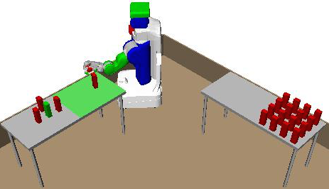
Many important planning domains naturally occur in continuous spaces involving complex constraints among variables. Consider planning for a robot tasked with organizing several blocks in a room. The robot must find a sequence of pick, place, and move actions involving continuous robot configurations, robot trajectories, block poses, and block grasps. These variables must satisfy highly non-linear kinematic, collision, and motion constraints which affect the feasibility of the actions. Each constraint typically requires a special purpose procedure to efficiently evaluate it or produce satisfying values for it such as an inverse kinematic solver, collision checker, or motion planner.
We propose an approach, called stripstream, which can model such a domain by providing a generic interface for blackbox procedures to be incorporated in an action language. The implementation of the procedures is abstracted away using streams: finite or infinite sequences of objects such as poses, configurations, and trajectories. We introduce the following two additional stream capabilities to effectively model domains with complex predicates that are only true for small sets of their argument values:
-
•
conditional streams: a stream of objects may be defined as a function of other objects; for example, a stream of possible positions of one object given the position of another object that it must be on top of or a stream of possible settings of parameters of a factory machine given desired properties of its output.
-
•
certified streams: streams of objects may be declared not only to be of a specific type, but also to satisfy an arbitrary conjunction of predicates; for example, one might define a certified conditional stream that generates positions for an object that satisfy requirements that the object be on a surface, that a robot be able to reach the object at that position, and that the robot be able to see the object while reaching.
Through streams, stripstream can compactly model a large class of continuous, countably infinite, and large finite domains. By conditioning on partial argument values and using sampling, it can even effectively model domains where the set of valid action argument values is lower dimensional than the possible argument space. For example, in our robotics domain, the set of inverse kinematics solutions for a particular pose and grasp is much lower dimensional than the full set of robot configurations. However, using a conditional stream, we can specify an inverse kinematics solver which directly samples from this set given a pose and grasp.
The approach is entirely domain-independent, and reduces to strips in the case of finite domains. The only additional requirement is the specification of a set of streams that can generate objects satisfying the static predicates in the domain. It is accompanied by two algorithms, a simple and a focused version, which operate by constructing and solving a sequence of strips planning problems. This strategy takes advantage of the highly optimized search strategies and heuristics that exist for strips planning, while expanding the domain of applicability of those techniques. Additionally, the focused version can efficiently solve problems where using streams is computationally expensive by carefully choosing to only call potentially useful streams.
Related work
There are a number of existing general-purpose approaches to solving planning problems in infinite domains, each of which has some significant limitation when modeling our robot domain.
Temporal planning, such as defined in pddl2.1 (?), is often formulated in terms of linear constraints on plan variables and is typically solved using techniques based on linear programming (?; ?). pddl+ (?) extends pddl2.1 by introducing exogenous events and continuous processes. Although pddl+ supports continuous variables, the values of continuous variables are functions of the sequence of discrete actions performed at particular times. Thus, time is the only truly non-dependent continuous variable. In contrast, our motivating robot domain has no notion of time but instead a continuously infinite branching factor. Many planners solve pddl+ problems with non-linear process models by discretizing time (?; ?). Some recent planners can solve pddl+ problems with polynomial process models exactly without time discretization (?; ?). However, even in simplified robotics domains that pddl+ can model, modern pddl+ planners are ineffective at planning with collision and kinematic constraints (both highly non-polynomial constraints), particularly in high-dimensional systems.
General-purpose lifted and first-order approaches, such as those based on first-order situation calculus or Prolog, provide semi-decision procedures for a large class of lifted planning problems. However, the generality tends to come at a huge price in efficiency and these planning strategies are rarely practical.
The Answer Set Programming (ASP) literature contains analysis on reasoning in infinite domains through finitary, -restricted, finitely ground, and finite domain ASPs (?). The DLV-Complex system (?) is able to solve feasible finitely ground programs by extending the DataLog with Disjunction (DLV) system to support functions, lists, and set terms. We believe that the language of ASP allows specification of conditional and certified streams. However, the ground ASP solver still has to address a much more general and difficult problem and will not have the appropriate heuristic strategies that make current domain-independent strips planners so effective.
Semantic attachments (?), predicates computed by an external program, also provide a way of integrating blackbox procedures and pddl planners. Because semantic attachments take a state as input, they can only be used in forward state-space search. Furthermore, semantic attachments are ignored in heuristics. This results in poor planner performance, particularly when the attachments are expensive to evaluate such as in robotics domains. Finally, because semantic attachments are restricted to be functions, they are unable to model domains with infinitely many possible successor states.
Many approaches to robotics planning problems, including motion planning and task-and-motion planning, have developed strategies for handling continuous spaces that go beyond a priori discretization. Several approaches, for example (?; ?; ?; ?; ?; ?), have been suggested for integrating these sampling-based robot motion planning methods with symbolic planning methods. Of these approaches, those able to plan in realistic robot domains have typically been quite special purpose; the more general purpose approaches have typically been less capable.
Representation
In this section we describe the representational components of a planning domain and problem, which include static and fluent predicates, operators, and streams. Objects serve as arguments to predicates and as parameters to operators; they are generated by streams.
A static predicate is a predicate which, for any tuple of objects, has a constant truth value throughout a problem instance. Static predicates generally serve to represent constraints on the parameters of an operator. We restrict static predicates to only ever be mentioned positively because, in the general infinite case, it is not possible to verify that a predicate does not hold.
An operator schema is specified by a tuple of formal parameters and conjunctions of static positive preconditions stat, fluent literal preconditions pre, and fluent literal effects eff and has the same semantics as in strips. An operator instance is a ground instantiation of an operator schema with objects substituted in for the formal parameters. When necessary, we augment the set of operator schemas with a set of axioms that naively use the same schema form as operators. We assume the set of axioms can be compiled into a set of derived predicates as used in pddl.
A generator is a finite or infinite sequence of object tuples . The procedure returns the next element in generator and returns the special object None to indicate that the stream has been exhausted and contains no more objects. A conditional generator is a function from to a generator which generates tuples from a domain not necessarily the same as the domain of .
An stream schema, , is specified by a tuple of input parameters , a tuple of output parameters , a conditional generator defined on , a conjunction of input static atoms inp defined on , and a conjunction of output static atoms out defined on and . The conditional generator is a function, implemented in the host programming language, that returns a generator such that, for all satisfying the conditions inp, satisfy the conditions out. A stream instance is a ground instantiation of a stream schema with objects substituted in for input parameters ; it is conditioned on those object values and, if the inp conditions are satisfied, then it will generate a stream of tuples of objects each of which satisfies the certification conditions out.
The notion of a conditional stream is quite general; there are two specific cases that are worth understanding in detail. An unconditional stream is a stream with no inputs whose associated function returns a single generator, which might be used to generate objects of a given type, for example, independent of whatever other objects are specified in a domain. A test stream is a degenerate, but still useful, type of stream with no outputs. In this case, contains either the single element , indicating that the inp conditions hold of , or contains no elements at all, indicating that the inp conditions do not hold of . It can be interpreted as an implicit Boolean test.
A planning domain is specified by finite sets of static predicates , fluent predicates , initial constant objects , operator schemas , axiom schemas , and stream schemas . Note that the initial objects (as well as objects generated by the streams) may in general not be simple symbols, but can be numeric values or even structures such as matrices or objects in an underlying programming language. They must provide a unique ID, such as a hash value, for use in the STRIPS planning phase.
A stripstream problem is specified by a planning domain , a finite set of initial objects , an initial state composed of a finite set of static or fluent atoms , and a goal set defined to be the set of states satisfying fluent literals . We make a version of the closed world assumption on the initial state , assuming that all true fluents are contained in it. This initial state will not be complete: in general, it will be impossible to assert all true static atoms when the universe is infinite.
Let and be the universe of all objects and the set of true initial atoms that can be generated from a finite set of stream schemas, a finite set of initial objects, and initial state . We give all proofs in the the appendix.
Theorem 1.
and are recursively enumerable (RE).
A solution to a stripstream problem is a finite sequence of operator instances with object parameters contained within that is applicable from and results in a state that satisfies . stripstream is undecidable but semi-decidable, so we restrict our attention to feasible instances.
Theorem 2.
The existence of a solution for a stripstream problem is undecidable.
Theorem 3.
The existence of a solution for a stripstream problem is semi-decidable.
Planning algorithms
We present two algorithms for solving stripstream problems: the incremental planner takes advantage of certified conditional streams in the problem specification to generate the necessary objects for solving the problem; the focused planner adds the ability to focus the object-generation process based on the requirements of the plan being constructed. Both algorithms are sound and complete: if a solution exists they will find it in finite time.
Both planners operate iteratively, alternating between adding elements and atoms to a current set of objects and initial atoms and constructing and solving strips planning problem instances. A strips problem is specified by a set of predicates, a set of operator schemas, a set of constant symbols, an initial set of atoms, and a set of goal literals. Let be any sound and complete planner for the strips subset of pddl. We implement s-plan using FastDownward (?).
Incremental planner
The incremental planner maintains a queue of stream instances and incrementally constructs set of objects and set of fluents and static atoms that are true in the initial state. The done set contains all streams that have been constructed and exhausted. In each iteration of the main loop, a strips planning instance is constructed from the current sets and , with the same predicates, operator and axiom schemas, and goal. If a plan is obtained, it is returned. If not, then attempts to add new objects are made where is a meta-parameter. In each one, a stream is popped from and a new tuple of objects is extracted from it. If the stream is exhausted, it is stored in . Otherwise, the objects in are added to , the output fluents from applied to are added to , and a new set of streams is constructed. For all stream schemas and possible tuples of the appropriate size , if the input conditions are in , then the instantiated stream is added to if it has not been added previously. We also return the stream to so we may revisit it in the future. The pseudo-code is shown below.
-
, while True: if : return if : return None for : if : continue for : for : if , :
In practice, many s-plan calls report infeasibility immediately because they have infinite admissible heuristic values. We prove the incremental algorithm is complete in the appendix.
Theorem 4.
The incremental algorithm is complete.
Focused planner
The focused planner is particularly aimed at domains for which it is expensive to draw an object from a stream; this occurs when the stream elements are certified to satisfy geometric properties such as being collision-free or having appropriate inverse kinematics relationships, for example. To focus the generation of objects on the most relevant parts of the space, we allow the planner to use “dummy” abstract objects as long as it plans to generate concrete values for them. These concrete values will be generated in the next iteration and will, hopefully, contribute to finding a solution with all ground objects.
As before, we transform the stripstream problem into a sequence of pddl problems, but this time we augment the planning domain with abstract objects, two new fluents, and a new set of operator schemas. Let be a set of abstract objects which are not assumed to satisfy any static predicates in the initial state. We introduce the fluent predicate , which is initially false for any object but true for all actual ground objects; so for all , we add to . The planner can “cause” an abstract object to satisfy by generating it using a special stream operator, as described below. We define procedure tform-ops that transforms each operator scheme by adding preconditions for to ensure that the parameters for are grounded before its application during the search.
To manage the balance in which streams are called, for each stream schema , we introduce a new predicate ; when applied to arguments , it will temporarily prevent the use of stream . Additionally, we add any new objects and static atoms first to sets and temporarily before adding them to and to ensure any necessary existing streams are called. Alternatively, we can immediately add directly to and a finite number of times before first adding to and and still preserve completeness. Let the procedure tform-streams convert each stream schema into an operator schema of the following form.
-
StreamOperator:
pre = eff =
It allows s-plan to explicitly plan to generate a tuple of concrete objects from stream as long as the have been made concrete and the stream instance is not blocked.
The procedure focused, shown below, implements the focused approach to planning. It takes the same inputs as the incremental version, but with the maximum number of abstract objects specified as a meta-parameter, rather than . It also maintains a set of concrete objects and a set of fluent and static atoms true in the initial state. In each iteration of the main loop, a strips planning instance is constructed: the initial state is augmented with the set of static atoms indicating which streams are blocked and fluents asserting that the objects in are concrete; the set of operator schemas is transformed as described above and augmented with the stream operator schemas, and the set of objects is augmented with the abstract objects. If a plan is obtained and it contains only operator instances, then it will have only concrete objects, and it can be returned directly. If the plan contains abstract objects, it also contains stream operators, and add-objects is called to generate an appropriate set of new objects. If no plan is obtained, and if no streams are currently blocked as well as no new objects or initial atoms have been produced since the last reset, then the problem is proved to be infeasible. Otherwise, the problem is reset by unblocking all streams and adding and to and , in order to allow a new plan with abstract objects to be generated.
-
; while True: if : if , : return else if : return None // Infeasible // Enable all objects & streams
Given a plan that contains abstract objects, we process it from beginning to end, to generate a collection of new objects with appropriate conditional relationships. Procedure add-objects initializes an empty binding environment and then loops through the instances of stream operators in . For each stream operator instance, we substitute concrete objects in for abstract objects, in the input parameters, dictated by the bindings , and then draw a new tuple of objects from that conditional stream. If there is no such tuple of objects, the stream is exhausted and it is permanently removed from future consideration by adding the fluent to the set . Otherwise, the new objects are added to and appropriate new static atoms to . This stream is temporarily blocked by adding fluent to the set , and the bindings for abstract objects are recorded.
-
// Empty dictionary for and : if : if : // Temporary for : else // Permanent return
The focused algorithm is similar to the lazy shortest path algorithm for motion planning in that it determines which streams to call, or analogously which edges to evaluate, by repeatedly solving optimistic problems (?; ?). Stream operators can be given meta-costs that reflect the time overhead to draw elements from the stream and the likelihood the stream produces the desired values. For example, stream operators that use already concrete outputs can be given large meta-costs because they will only certify a desired predicate in the typically unlikely event that their generator returns objects matching the desired outputs. A cost-sensitive planner will avoid returning plans that require drawing elements from expensive or unnecessary streams. We can combine the behaviors of incremental and focused algorithms to eagerly call inexpensive streams and lazily call expensive streams. This can be seen as automatically applying some stream operators before calling s-plan.
Theorem 5.
The focused algorithm is complete.
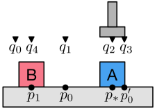
Example discrete domain
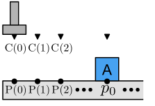
Although the specification language is domain independent, our primary motivating examples for the application of stripstream are pick-and-place problems in infinite domains. We start by specifying an infinite discrete pick-and-place domain as shown in figure 2. We purposefully describe the domain in a way that will generalize well to continuous and high-dimensional versions of fundamentally the same problem. The objects in this domain include a finite set of blocks (that can be picked up and placed), an infinite set of poses (locations in the world) indexed by the positive integers, and an infinite set of robot configurations (settings of the robot’s physical degrees of freedom) also indexed by the positive integers. In this appendix, we give a complete Python implementation of this domain in stripstream The static predicates in this domain include simple static types (, , ) and typical fluents (, , , ). In addition, atoms of the form describe a static relationship between an object pose and a robot configuration : in this simple domain, the atom is true if and only if . Finally, fluents of the form are true in the circumstance that: if object were placed at pose , it would not collide with object at its current pose. Because the set of blocks B is known statically in advance, we explicitly include all the conditions. These predicate definitions enable the following operator schemas definitions:
-
Move:
stat = pre = eff =
-
Pick:
stat = pre = eff =
-
Place:
stat = pre = eff =
We use the following axioms to evaluate the predicate. We need two slightly different definitions to handle the cases where the block is placed at a pose, and where it is in the robot’s hand. The axioms mention each block independently which allows us to compactly perform collision checking. Without using axioms, Place would require a parameter for the pose of each block in , resulting in an prohibitively large grounded problem.
-
SafeAxiom:
stat = pre = eff =
-
SafeAxiomH:
stat = pre = eff =
Discrete stream specification
Next, we provide stream definitions. The simplest stream is an unconditional generator of poses, which are represented as objects and satisfy the static predicate .
-
Pose-U:
gen = inp = out =
The conditional stream CFree-T is a test, calling the underlying function ; the stream is empty if block at pose collides with block at pose , and contains the single element if it does not collide. It is used to certify that the tuple statically satisfies the predicate.
-
CFree-T:
gen = inp = out =
When we have a static relation on more than one variable, such as , we have to make modeling choices when defining streams that certify it.
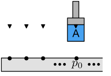
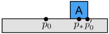
We will consider three formulations of streams that certify and compare them in terms of their effectiveness in a simple countable pick-and-place problem requiring the robot gripper to pick block at a distant initial pose , shown in figure 2.
Kin-U specifies an unconditional stream on block poses and robot configurations; it has no difficulty certifying the relation between the two output variables, but it has no good way of producing configurations that are appropriate for poses that are mentioned in the initial state or goal.
-
Kin-U:
gen = inp out =
Kin-T specifies a test stream that can be used, together with the Pose-U stream and an analogous stream for generic configurations to produce certified kinematic pairs . This is an encoding of a “generate-and-test” strategy, which may be highly inefficient, relying on luck that the pose generator and the configuration generator will independently produce values that have the appropriate relationship.
-
Kin-T:
gen = inp = out =
Finally, Kin-C specifies a conditional stream, which takes a pose as input and generates a stream of configurations (in this very simple case, containing a single element) certified to satisfy the relation. It relies on an underlying function to produce an appropriate robot configuration given a block pose.
-
Kin-C:
gen = inp = out =
In our example domain, both Kin-U and Kin-T require the enumeration of poses and configurations from before certifying , allowing strips to make a plan include the operator . Moreover, Kin-T will test all pairs of configurations and poses. In contrast, Kin-C can produce directly from without enumerating any other poses or configurations. The conditional formulation is advantageous because it produces a paired inverse kinematics configuration quickly and without substantially expanding the size of the problem.
Table 1 validates this intuition though an experiment comparing these stream specifications. The initial pose of the object is chosen from . All trials have a timeout of 120 seconds and use the incremental algorithm with implemented in Python. As predicted, the Kin-U and Kin-T streams require many more calls than Kin-C as increases and lead to substantially longer runtimes for a very simple problem.
| Kin-U | Kin-T | Kin-C | |||||||
| t | i | c | t | i | c | t | i | c | |
| 1 | .1 | 3 | 2 | .2 | 6 | 9 | .1 | 3 | 2 |
| 100 | 29 | 102 | 101 | 71 | 303 | 10360 | .1 | 3 | 2 |
| 1000 | - | 180 | 179 | - | 381 | 16383 | .1 | 3 | 2 |
Continuous domains
The stripstream approach can be applied directly in continuous domains such as the problem in figure 3. In this case, the streams will have to generate samples from sets of continuous dimensions, and the way that samples are generated may have a significant impact on the efficiency and completeness of the approach with respect to the domain problem. (Note that the stripstream planing algorithms are complete with respect to the streams of enumerated values they are given, but if these value streams are not, in some sense, complete with respect to the underlying problem domain, then the resulting combined system may not be complete with respect to the original problem.) Samplers that produce a dense sequence (?) are good candidates for stream generation.
Continuous stream specification
With some minor modifications, we can extend our discrete pick-and-place domain to a bounded interval of the real line. Poses and configurations are now continuous objects from an uncountably infinite domain. The stream Pose-U now has a generator that samples uniformly at random.
While in the discrete case the choice of streams just affected the size of the problem, in the continuous case, the choice of streams can affect the feasibility of the problem. In the continuous simple pick-and-place domain, suppose that the blocks have width 1 and the gripper has width . A kinematics pair is valid if and only if the gripper is entirely over the block, i.e., and . Consider the case where Kin-U and Kin-C are implemented using random samplers. Kin-U will almost certainly generate a sequence of infeasible strips problems, because the probability that the point is produced from its generator is zero. For , the configuration stream has nonzero probability of generating a that would constitute a valid kinematics pair with as certified by Kin-T. But this probability can be made arbitrary small as . Only the Kin-C strategy is robust to the choice of . Table 2 shows the results of an experiment analogous to the one in table 1, but which varies instead of varying . Kin-U was unable to solve either problem and Kin-T could not find a solution in under two minutes for . But once again, the conditional formulation using Kin-C performs equivalently for different values of .
| Kin-U | Kin-T | Kin-C | |||||||
|---|---|---|---|---|---|---|---|---|---|
| t | i | c | t | i | c | t | i | c | |
| 1.5 | - | 191 | 190 | 3.1 | 75 | 745 | .1 | 2 | 1 |
| 1.01 | - | 181 | 180 | - | 297 | 18768 | .1 | 2 | 1 |
Focused algorithm example
The previous examples investigated the effect of different representational choices on the tractability and even feasibility of the resulting stripstream problem.
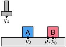
The example in figure 3 illustrates the behavior of the focused algorithm on continuous a pick-and-place problem with the goal condition that block is at pose . Because block A, when at , collides with block B at its initial pose , solving this problem requires moving block out of the way to place block . Suppose we use Kin-C to model the problem. We will omit Move operators for the sake of clarity, and use capital letters to denote abstract objects. On the first iteration, the focused algorithm will produce the following plan (possibly ordered slightly differently):
The generation of values proceeds as follows. will produce . will produce . However, will produce the empty stream because collides with . Thus, the plan definitively cannot be completed. The algorithm adds and to the current pddl problem and records the failure of . On the next iteration, the focused algorithm will produce the following plan.
The generation of values proceeds as follows. will produce . will produce . will produce . Let’s assume that is randomly sampled and turns out to not be in collision with . If turned out to be in collision with , the next iteration would first fail once, then repeat this process on the next iteration to generate a new . So, will produce the stream indicating that and are not in collision. Thus, all of the properties have been successfully satisfied, so the following plan is a solution. It is critical to note that, for example, had there been several other pose constants appearing in the initial state, focused would never have found inverse kinematic solutions for them: because the planner guides the sampling, only stream elements that play a direct role in a plausible plan are generated.
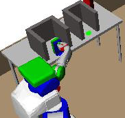
Realistic robot domain
| incremental, | incremental, | focused | ||||||||||
| % | t | i | c | % | t | i | c | % | t | i | c | |
| 1 | 88 | 2 | 23 | 268 | 68 | 5 | 2 | 751 | 84 | 11 | 6 | 129 |
| 2-0 | 100 | 23 | 85 | 1757 | 100 | 9 | 3 | 2270 | 100 | 2 | 3 | 180 |
| 2-8 | 0 | - | - | - | 100 | 55 | 5 | 17217 | 100 | 7 | 3 | 352 |
| 2-16 | 0 | - | - | - | 100 | 112 | 6 | 36580 | 100 | 19 | 3 | 506 |
Finally, we extend our continuous pick-and-place to the high-dimensional setting of a robot operating in household-like environments. Poses of physical blocks are 6-dimensional and robot configurations are 11-dimensional. We introduce two new object types: grasps and trajectories. Each block has a set of 6D relative grasp transforms at which it can be grasped by the robot. Trajectories are finite sequences of configuration waypoints which must be included in collision checking. The extended Pick operator, CFree-T test and Kin-C stream templates are:
-
Pick:
stat = pre = eff =
-
CFree-T:
gen = inp = out =
-
Kin-C:
gen = inp = out =
Pick adds grasp and trajectory as parameters and includes preconditions to verify that while holding at grasp is safe with respect to each other block . is updated using SafeAxiom which has a static precondition. Here, a collision check for block at pose is performed for each configuration in . Instead of simple blocks, physical objects in this domain are general unions of convex polygons. Although checking collisions here is more complication than in 1D, it can be treated in the same way, as an external function.
The Kin streams must first produce a grasp configuration that reaches manipulator transform using inverse-kin. Additionally, they include a motion planner motions to generate legal trajectory values from a constant rest configuration to the grasping configuration that do not collide with the fixed environment. In this domain, the procedures for collision checking and finding kinematic solutions are significantly more involved and computationally expensive than in the previous domains, but their underlying function is the same.
Experiments
We applied the incremental and focused algorithms on four challenging pick-and-place problems to demonstrate that a general-purpose representation and algorithms can be used to achieve good performance in difficult problems. For both algorithms, test streams are always evaluated as soon as they are instantiated. We experimented on two domains shown in figure 4, which are similar to problems introduced by (?). The first domain, in which problem 1 is defined, has goal conditions that the green object be in the right bin and the blue object remain at its initial pose. This requires the robot to not only move and replace the blue block but also to place the green object in order to find a new grasp to insert it into the bin. The second domain, in which problems 2-0, 2-8, and 2-16 are defined, requires moving an object out of the way and placing the green object in the green region. For problem 2- where there are other blocks on a separate table that serve as distractors. The streams were implemented using the OpenRAVE robotics framework (?). A Python implementation of stripstream can be found here: https://github.com/caelan/stripstream.
The results compare the incremental algorithm where and with the focused algorithm. Table 3 shows the results of 25 trials, each with a timeout of 120 seconds. The incremental algorithms result in significantly more stream calls than the focused algorithm. These calls can significantly increase the total runtime because each inverse kinematic and collision primitive itself is expensive. Additionally, the incremental algorithms are significantly affected by the increased number of distractors, making them unsuitable for complex real-world environments. The focused algorithm, however, is able to selectively choose which streams to call resulting in significantly better performance in these environments.
Conclusion
The stripstream problem specification formalism can be used to describe a large class of planning problems in infinite domains and provides a clear and clean interface to problem-specific sampling methods in continuous domains. The incremental and, in particular, focused planning algorithms take advantage of the specification to provide efficient solutions to difficult problems.
References
- [Bohlin and Kavraki 2000] Robert Bohlin and Lydia E Kavraki. Path planning using lazy PRM. In IEEE International Conference on Robotics and Automation (ICRA), volume 1, pages 521–528. IEEE, 2000.
- [Bonatti et al. 2010] Piero Bonatti, Francesco Calimeri, Nicola Leone, and Francesco Ricca. Answer set programming. In A 25-year perspective on logic programming, pages 159–182. Springer-Verlag, 2010.
- [Bryce et al. 2015] Daniel Bryce, Sicun Gao, David J Musliner, and Robert P Goldman. SMT-based nonlinear PDDL+ planning. In AAAI, 2015.
- [Calimeri et al. 2009] Francesco Calimeri, Susanna Cozza, Giovambattista Ianni, and Nicola Leone. An asp system with functions, lists, and sets. In International Conference on Logic Programming and Nonmonotonic Reasoning, pages 483–489. Springer, 2009.
- [Cashmore et al. 2016] Michael Cashmore, Maria Fox, Derek Long, and Daniele Magazzeni. A compilation of the full pddl+ language into smt. In International Conference on Automated Planning and Scheduling (ICAPS), pages 79–87. AAAI Press, 2016.
- [Coles et al. 2013] Amanda Coles, Andrew Coles, Maria Fox, and Derek Long. A hybrid LP-RPG heuristic for modelling numeric resource flows in planning. Journal of Artificial Intelligence Research (JAIR), 46(1):343–412, 2013.
- [Dantam et al. 2016] Neil T. Dantam, Z. Kingston, Swarat Chaudhuri, and Lydia E. Kavraki. Incremental task and motion planning: A constraint-based approach. In Robotics: Science and Systems (RSS), 2016.
- [Della Penna et al. 2009] Giuseppe Della Penna, Daniele Magazzeni, Fabio Mercorio, and Benedetto Intrigila. Upmurphi: A tool for universal planning on pddl+ problems. In International Conference on Automated Planning and Scheduling (ICAPS), 2009.
- [Dellin and Srinivasa 2016] Christopher M Dellin and Siddhartha S Srinivasa. A unifying formalism for shortest path problems with expensive edge evaluations via lazy best-first search over paths with edge selectors. International Conference on Automated Planning and Scheduling (ICAPS), 2016.
- [Diankov and Kuffner 2008] Rosen Diankov and James Kuffner. Openrave: A planning architecture for autonomous robotics. Technical Report CMU-RI-TR-08-34, Robotics Institute, Carnegie Mellon University, 2008.
- [Dornhege et al. 2009] Christian Dornhege, Patrick Eyerich, Thomas Keller, Sebastian Trüg, Michael Brenner, and Bernhard Nebel. Semantic attachments for domain-independent planning systems. In International Conference on Automated Planning and Scheduling (ICAPS), pages 114–121. AAAI Press, 2009.
- [Erdem et al. 2011] Esra Erdem, Kadir Haspalamutgil, Can Palaz, Volkan Patoglu, and Tansel Uras. Combining high-level causal reasoning with low-level geometric reasoning and motion planning for robotic manipulation. In IEEE International Conference on Robotics and Automation (ICRA), 2011.
- [Fox and Long 2003] Maria Fox and Derek Long. Pddl2.1: An extension to PDDL for expressing temporal planning domains. Journal of Artificial Intelligence Research (JAIR), 20:2003, 2003.
- [Fox and Long 2006] Maria Fox and Derek Long. Modelling mixed discrete-continuous domains for planning. J. Artif. Intell. Res.(JAIR), 27:235–297, 2006.
- [Garrett et al. 2015] Caelan Reed Garrett, Tomás Lozano-Pérez, and Leslie Pack Kaelbling. Backward-forward search for manipulation planning. In IEEE/RSJ International Conference on Intelligent Robots and Systems (IROS), 2015.
- [Garrett et al. 2016] Caelan Reed Garrett, Tomas Lozano-Perez, and Leslie Pack Kaelbling. FFRob: Leveraging symbolic planning for efficient task and motion planning. arXiv preprint arXiv:1608.01335, 2016.
- [Helmert 2006] Malte Helmert. The fast downward planning system. Journal of Artificial Intelligence Research (JAIR), 26:191–246, 2006.
- [Hoffmann and others 2003] Jörg Hoffmann et al. The Metric-FF planning system: Translating ”ignoring delete lists” to numeric state variables. J. Artif. Intell. Res.(JAIR), 20:291–341, 2003.
- [Kaelbling and Lozano-Pérez 2011] Leslie Pack Kaelbling and Tomás Lozano-Pérez. Hierarchical planning in the now. In IEEE International Conference on Robotics and Automation (ICRA), 2011.
- [LaValle 2006] Steven M. LaValle. Planning Algorithms. Cambridge University Press, 2006.
- [Piotrowski et al. 2016] Wiktor Piotrowski, Maria Fox, Derek Long, Daniele Magazzeni, and Fabio Mercorio. Heuristic planning for pddl+ domains. In Proceedings of the Twenty-Fifth International Joint Conference on Artificial Intelligence (IJCAI), 2016.
- [Srivastava et al. 2014] Siddharth Srivastava, Eugene Fang, Lorenzo Riano, Rohan Chitnis, Stuart Russell, and Pieter Abbeel. Combined task and motion planning through an extensible planner-independent interface layer. In IEEE International Conference on Robotics and Automation (ICRA), 2014.
Appendix
Theorem 6.
and are recursively enumerable (RE).
Proof.
Consider an enumeration procedure for and :
-
•
The first sequences of elements in and are and respectively.
-
•
Initialize a set of stream instances .
-
•
Repeat:
-
–
For each stream schema , add all instantiations where such that is contained within , to . There are finitely many new elements of .
-
–
For each stream instance , add to and add to . There are finitely many new elements of and .
-
–
This procedure will enumerate all possible objects and all possible initial atoms generated within the problem . ∎
Theorem 7.
The existence of a solution for a stripstream problem is undecidable.
Proof.
We use a reduction from the halting problem. Given a Turning machine TM, we construct a stripstream problem with a single operator Halt(X) with , , and where and are a static and fluent predicate defined on TM’s states. There is a single unconditional stream which enumerates the states of TM by simulating one step of TM upon each call. Let and where is the accept state for TM. has a solution if and only if TM halts. Thus, stripstream is undecidable. ∎
Theorem 8.
The existence of a solution for a stripstream problem is semi-decidable.
Proof.
From the recursive enumeration of and we produce a recursive enumeration of finite planning problems. Planning problem is grounded using all objects and static atoms enumerated up through element . Plan existence in a finite universe is decidable. Thus, for feasible problems, applying a finite decision procedure to the sequence of finite planning problems will eventually reach a planning problem for which a plan exists and produce it. ∎
Theorem 9.
The incremental algorithm is complete.
Proof.
The incremental algorithm constructs and in the same way as theorem 6 for and except that it calls next in batches of . Thus, any finite subsets of and will be included in and after a finite number of iterations. Let be a solution to a feasible stripstream problem . Consider the first iteration where and contain the set of objects used along and static atoms supporting . On that iteration, s-plan will return some solution (if not ) in finite time because it is sound and complete. ∎
Theorem 10.
The focused algorithm is complete.
Proof.
Define an episode as the focused algorithm iterations between the last reset () and the next reset. Consider a minimum length solution to a feasible stripstream problem . Let be the set of objects used along and be the set of static atoms supporting .
For each episode, consider the following argument. By theorem 6, there exists a sequence of stream instance calls which produces and from the current and . Let be the minimum length sequence that satisfies this property. may include the same stream instance several times if multiple calls are needed to produce the necessary values. On each iteration, focused creates a finite strips problem by augmenting with the abstract objects and the stream operators . Because and are withheld, and are fixed for all iterations within the episode. Thus, a finite number of simple plans are solutions for . One of these plans, , is concatenated with where additionally any object is replaced with some abstract object . Assume all redundant stream operators are removed from . The same can stand in for several on at once. Thus, focused will be complete for any .
We will show that at least one stream instance in will called performed during each episode. On each iteration, s-plan will identify a plan . If does not involve any abstract objects and is fully supported, it is a solution. Otherwise, add-objects will call each stream associated with . It adds to , preventing and all other plans using from being re-identified within this episode. If overlaps with and , then the episode has succeeded. Otherwise, this process repeats on the next iteration. Eventually a stream instance in will be called, or itself will be the only remaining unblocked plan for . In which case, s-plan will return , and add-objects will call a stream instance in .
strictly decreases after each episode. Inductively applying this, after a finite number of episodes, and . During the next episode, s-plan will be guaranteed to return some solution (if not ).
∎
Python example discrete domain
Figure 5 gives a complete encoding of the example discrete domain and a problem instance within it using our Python implementation of stripstream. In the specified problem instance, the initial state consists of three blocks placed in a row. The goal is to shift each of the blocks over one pose. The Python syntax of stripstream intentionally resembles the Planning Domain Definition Language (pddl) (?). We use several common features of pddl that extend strips. The resulting encoding is equivalent to previously described strips formulation but is more compact. We use object types BLOCK, POSE, CONF instead of static predicates , , and . Additionally, we use several Action Description Language (ADL) logical operations including Or, Equal, ForAll, and Exists. The universal quantifier (ForAll) is over BLOCK, a finite type, and thus is a finite conjunction.
from stripstream import Type, Param, Pred, Not, Or, And, Equal, Exists, \ ForAll, Action, Axiom, GeneratorStream, TestStream, STRIPStreamProblemblocks = [’block%i’%i for i in range(3)]num_poses = pow(10, 10) # a very large number of posesinitial_config = 0 # initial robot configuration is 0initial_poses = {block: i for i, block in enumerate(blocks)} # initial pose for block i is igoal_poses = {block: i+1 for i, block in enumerate(blocks)} # goal pose for block i is i+1BLOCK, POSE, CONF = Type(), Type(), Type() # Object typesB1, B2 = Param(BLOCK), Param(BLOCK) # Free parametersP1, P2 = Param(POSE), Param(POSE)Q1, Q2 = Param(CONF), Param(CONF)AtConf = Pred(CONF) # Fluent predicatesAtPose = Pred(BLOCK, POSE)HandEmpty = Pred()Holding = Pred(BLOCK)Safe = Pred(BLOCK, BLOCK, POSE) # Derived predicatesIsKin = Pred(POSE, CONF) # Static predicatesIsCollisionFree = Pred(BLOCK, POSE, BLOCK, POSE)actions = [ Action(name=’pick’, parameters=[B1, P1, Q1], condition=And(AtPose(B1, P1), HandEmpty(), AtConf(Q1), IsKin(P1, Q1)), effect=And(Holding(B1), Not(AtPose(B1, P1)), Not(HandEmpty()))), Action(name=’place’, parameters=[B1, P1, Q1], condition=And(Holding(B1), AtConf(Q1), IsKin(P1, Q1), ForAll([B2], Or(Equal(B1, B2), Safe(B2, B1, P1)))), effect=And(AtPose(B1, P1), HandEmpty(), Not(Holding(B1)))), Action(name=’move’, parameters=[Q1, Q2], condition=AtConf(Q1), effect=And(AtConf(Q2), Not(AtConf(Q1))))]axioms = [ Axiom(effect=Safe(B2, B1, P1), # Infers B2 is at a safe pose wrt B1 at P1 condition=Exists([P2], And(AtPose(B2, P2), IsCollisionFree(B1, P1, B2, P2))))]cond_streams = [ GeneratorStream(inputs=[], outputs=[P1], conditions=[], effects=[], generator=lambda: xrange(num_poses)), # Enumerates all the poses GeneratorStream(inputs=[P1], outputs=[Q1], conditions=[], effects=[IsKin(P1, Q1)], generator=lambda p: [p]), # Inverse kinematics TestStream(inputs=[B1, P1, B2, P2], conditions=[], effects=[IsCollisionFree(B1, P1, B2, P2)], test=lambda b1, p1, b2, p2: p1 != p2)] # Collision checkingconstants = []initial_atoms = [AtConf(initial_config), HandEmpty()] + \ [AtPose(block, pose) for block, pose in initial_poses.iteritems()]goal_formula = And(AtPose(block, pose) for block, pose in goal_poses.iteritems())return STRIPStreamProblem(initial_atoms, goal_formula, actions+axioms, cond_streams, constants)