A hybrid finite volume – finite element method for bulk–surface coupled problems

Abstract

The paper develops a hybrid method for solving a system of advection–diffusion equations in a bulk domain coupled to advection–diffusion equations on an embedded surface. A monotone nonlinear finite volume method for equations posed in the bulk is combined with a trace finite element method for equations posed on the surface. In our approach, the surface is not fitted by the mesh and is allowed to cut through the background mesh in an arbitrary way. Moreover, a triangulation of the surface into regular shaped elements is not required. The background mesh is an octree grid with cubic cells. As an example of an application, we consider the modeling of contaminant transport in fractured porous media. One standard model leads to a coupled system of advection–diffusion equations in a bulk (matrix) and along a surface (fracture). A series of numerical experiments with both steady and unsteady problems and different embedded geometries illustrate the numerical properties of the hybrid approach. The method demonstrates great flexibility in handling curvilinear or branching lower dimensional embedded structures.

Keywords: Finite volume method, TraceFEM, bulk–surface coupled problems, fractured porous media, unfitted meshes, octree grid

1 Introduction

Systems of coupled bulk–surface partial differential equations arise in many engineering and natural science applications. Examples include multiphase fluid dynamics with soluble or insoluble surfactants [25], dynamics of biomembranes [7], crystal growth [29], signaling in biological networks [46], and transport of solute in fractured porous media [1]. In these and other applications, partial differential equations defined in a volume domain are coupled to another PDEs posed on a surface. The surface may be embedded in the bulk or belong to a boundary of the volume domain.

Recently, there has been a growing interest in developing methods for the numerical treatment of bulk–surface coupled PDEs. Different approaches can be distinguished depending on how the surface is recovered and equations are treated. If a tessellation of the volume into tetrahedra is available that fits the surface, then it is natural to introduce finite element spaces in the volume and on the induced triangulation of the surface. The resulting fitted bulk–surface finite element method was studied for the stationary bulk–surface advection–diffusion equations [18], for non-linear reaction–diffusion systems modelling biological pattern formation [36, 37], for the equations of the two–phase flow with surfactants [5, 4], Darcy and transport–diffusion equations in fractured porous media [1].

Unfitted finite element methods allow the surface to cut through the background tetrahedral mesh. In the class of finite element methods also known as cutFEM, Nitsche-XFEM or TraceFEM, standard background finite element spaces are employed, while the integration is performed over cut domains and over the embedded surface  [8, 44]. Additional stabilization terms are often added to ensure the robustness of the method with respect to small cut elements. The advantages of the unfitted approach are the efficiency in handling implicitly defined surfaces, complex geometries, and the flexibility in dealing with evolving domains. In the context of bulk–surface coupled problems, cut finite element methods were recently applied to treat stationary bulk–surface advection–diffusion equations [24], coupled bulk-surface problems on time-dependent domains [26], coupled elasticity problems [9]. The hybrid method developed in this paper belongs to the general class of unfitted methods and resembles the TraceFEM in how the surface PDE is treated.

The methods discussed above treat surfaces and interfaces sharply, i.e. as lower-dimensional manifolds. In the present paper we also consider sharp interfaces. For the application of phase–field or other diffuse-interface approaches for coupled bulk–surface PDEs see, for example, [10, 33, 51].

If the finite element method is a discretization of choice for the bulk problem, then it is natural to consider a finite element method for surface PDE as well. However, depending on application, desired conservation properties, available software or personal experience, other discretizations such as finite volume or finite difference methods can be preferred for the PDE posed in the volume. One possibility to reuse the same mesh for the surface PDE is to consider a diffuse-interface approach. Alternatively, instead of smearing the interface, one may extend the PDE off the surface to a narrow band containing the surface in such a way that the restriction of the extended PDE solution back to the (sharp) surface solves the original equation on this surface. Further a conventional discretization is built for the resulting volume PDE in the narrow band  [6, 43]. The methods based on such extensions, however, increase the number of the active degrees of freedom for the discrete surface problem, may lead to degenerated PDE, need numerical boundary conditions and require smooth surfaces with no geometrical singularities.

The present paper develops a numerical method based on the sharp-interface representation, which uses a finite volume method to discretize the bulk PDE. Our goal is (i) to allow the surface to overlap with the background mesh in an arbitrary way, (ii) to avoid building regular surface triangulation, (iii) to avoid any extension of the surface PDE to the bulk domain. To accomplish these goals, we combine the monotone (i.e. satisfying the discrete maximum principle) finite volume method on general meshes [35, 11] with the trace finite element method on octree meshes from [12]. In the octree TraceFEM one considers the bulk finite element space of piecewise trilinear globally continuous functions and further uses the restrictions (traces) of these functions to the surface. These traces are further used in a variational formulation of the surface PDE. Effectively, this results in the integration of the standard polynomial functions over the (reconstructed) surface. Only degrees of freedom from the cubic cells cut by the surface are active for the surface problem. Surface parametrization is not required, no surface mesh is built, no PDE extension off the surface is needed. We shall see that the resulting hybrid FV–FE method is very robust with respect to the position of surfaces against the background mesh and is well suited for handling non-smooth surfaces and surfaces given implicitly.

One application of interest is the numerical simulation of the contaminant transport and diffusion in fractured porous media. In this application, transport and diffusion along fractures are often modeled by PDEs posed on a set of piecewise-smooth surfaces, see, e.g., [1, 22, 39, 52]; see also [1, 2, 38, 20] for a similar dimension reduction approach in simulation of flow in fractured porous media. Monotone (satisfying the DMP) finite volume methods on general meshes is the appealing tool for the solution of equations for solute concentration in the porous matrix, see, e.g.,  [11, 17, 23, 28, 30, 35, 49] (further references can be found in [16, 21]). However, a straightforward application of this technique to model transport and diffusion along a fracture would require fitting the mesh or triangulating the surface. For a large and complex net of fractures cutting through the porous matrix this is a difficult task [14], and an efficient method avoids mesh fitting and surface triangulations. Recently, extended finite element method approximations have been extensively studied in transport and flow problems in fractured porous media, see the review [19] and references therein. In XFEM, one also avoids fitting of the background mesh to a fracture, but a separate mesh is still required to represent the fracture. Besides the use of FV for the matrix problem, the approach in the present paper differs from those found in existing XFEM literature in the way the surface problem is discretized.

While the present technique can be applied for tetrahedral or more general polyhedral tessellations of the bulk domain, we consider octree grid with cubic cells here. This choice is not ad hoc. Indeed, the Cartesian structure and built-in hierarchy of octree grids makes mesh adaptation, reconstruction and data access fast and easy. For these reasons, octree meshes became a common tool in in computational mechanics and several octree-based solvers are available in the open source scientific computing software, [3, 45]. However, an octree grid provides at most the first order (staircase) approximation of a general geometry. Allowing the surface to cut through the octree grid in an arbitrary way overcomes this issue, but challenges us with the problem of building efficient bulk–surface discretizations. This paper demonstrates that the hybrid TraceFEM – non-linear FV method complements the advantages of using octree grids by delivering more accurate treatment of the surface PDE problem.

The remainder of the paper is organized as follows. In section 2 we recall the system of differential equations, boundary and interface conditions, which models the coupled bulk–interface (or “matrix–fracture” in the context of flows in porous media) advection–diffusion problem. Section 3 gives the details of the hybrid discretization. After laying out the main ideas behind the method, we discuss the non-linear monotone FV method for the bulk and the TraceFEM for the surface equations, and further we introduce the required coupling. Section 4 presents the results of several numerical experiments with steady analytical solutions on smooth and piecewise smooth branching surface. We also show the results of numerical simulation of the propagating front of solute concentration through fractured porous media.

2 Mathematical model

In this section we recall the mathematical model of the contaminant diffusion and transport in fractured porous media. Assume the given bulk domain $\Omega\subset\mathbb{R}^{3}$ and a piecewise smooth surface $\Gamma\subset\Omega$. The surface $\Gamma$ may have several connected components. If $\Gamma$ has a boundary, we assume that ${\partial\Gamma}\subset{\partial\Omega}$. Thus, we have the subdivision $\overline{\Omega}=\cup_{i=1,\dots,N}\overline{\Omega}_{i}$ into simply connected subdomains $\Omega_{i}$ such that $\overline{\Omega}_{i}\cap\overline{\Omega}_{j}\subset\Gamma$, $i\neq j$.

In each $\Omega_{i}$, we assume a given Darcy velocity field of the fluid $\mathbf{w}_{i}(\mathbf{x})$, $\mathbf{x}\in\Omega_{i}$. By $\mathbf{w}_{\Gamma}(\mathbf{x})$, $\mathbf{x}\in{\color[rgb]{0,0,0}{\Gamma}}$, we denote the velocity field tangential to $\Gamma$ having the physical meaning of the flow rate through the cross-section of the fracture. Consider an agent that is soluble in the fluid and transported by the flow in the bulk and along the fractures. The fractures are modeled by the surface $\Gamma$. The solute volume concentration (i.e., the one in the bulk domain $\Omega$) is denoted by $u$, $u_{i}=u|_{\Omega_{i}}$. The solute surface concentration along $\Gamma$ is denoted by $v$. Change of the concentration happens due to convection by the velocity fields $\mathbf{w}_{i}$ and $\mathbf{w}_{\Gamma}$, diffusive fluxes in $\Omega_{i}$, diffusive flux on $\Gamma$, as well as the fluid exchange and diffusion flux between the fractures and the porous matrix. These coupled processes can be modeled by the following system of equations [1], in subdomains,

$$\left\{\begin{aligned} \phi_{i}\frac{\partial u_{i}}{\partial t}+\mbox{\rm div}(\mathbf{w}_{i}u_{i}-D_{i}\nabla u_{i})&=f_{i}\quad\text{in}~{}\Omega_{i},\\ u_{i}&=v\quad\text{on}~{}{\partial\Omega}_{i}\cap\Gamma,\end{aligned}\right.$$ (1)

and on the surface,

$$\phi_{\Gamma}\frac{\partial v}{\partial t}+\mbox{\rm div}_{\Gamma}(\mathbf{w}_{\Gamma}v-dD_{\Gamma}\nabla_{\Gamma}v)=F_{\Gamma}(u)+f_{\Gamma}\quad\text{on}~{}~{}\Gamma,$$ (2)

where we employ the following notations: $\nabla_{\Gamma}$, $\mbox{\rm div}_{\Gamma}$ denote the surface tangential gradient and divergence

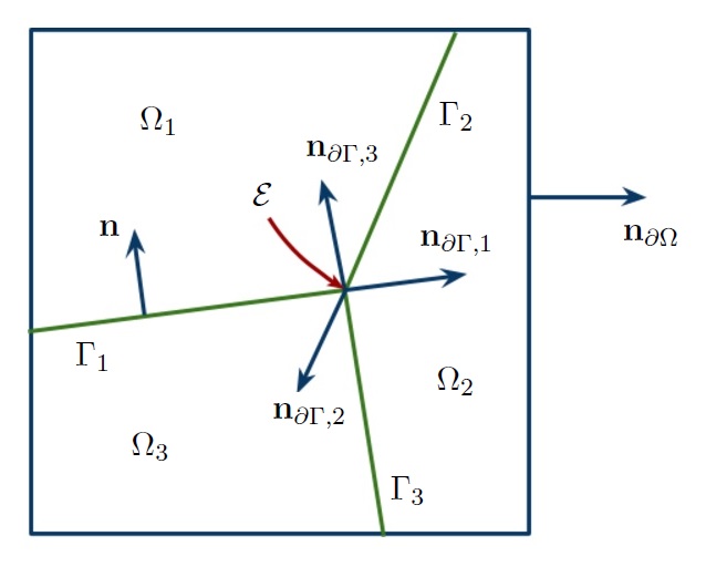
Figure 1: 2D illustration of our notation for a domain with triple fraction.

operators; $F_{\Gamma}(u)$ stands for the net flux of the solute per surface area due to fluid leakage and hydrodynamic dispersion; $f_{i}$ and $f_{\Gamma}$ are given source terms in the subdomains and in the fracture; $D_{i}$ denotes the diffusion tensor in the porous matrix; the surface diffusion tensor is $D_{\Gamma}$. Both $D_{i}$, $i=1,\dots,N$, and $D_{\Gamma}$ are symmetric and positive definite; $d>0$ is the fracture width coefficient; $\phi_{i}>0$ and $\phi_{\Gamma}>0$ are the constant porosity coefficients for the bulk and the fracture.

The total surface flux $F_{\Gamma}(u)$ represents the contribution of the bulk to the solute transport in the fracture. The mass balance at $\Gamma$ leads to the equation

$$F_{\Gamma}(u)=[-D\mathbf{n}\cdot\nabla u+(\mathbf{n}\cdot\mathbf{w})u]_{\Gamma},$$ (3)

where $\mathbf{n}$ is a unit normal vector at $\Gamma$, $[w(\mathbf{x})]_{\Gamma}=\lim\limits_{\varepsilon\to 0}w(\mathbf{x}-\varepsilon\mathbf{n})-\lim\limits_{\varepsilon\to 0}w(\mathbf{x}+\varepsilon\mathbf{n})$, $\mathbf{x}\in\Gamma$, denotes the jump of $w$ across $\Gamma$ in the direction of $\mathbf{n}$.

If $\Gamma$ is piecewise smooth, then we need further conditions on the edges. Assume an edge $\mathcal{E}$ is shared by $M$ smooth components $\Gamma_{i}\subset\Gamma$. Let $v_{j}=v$ on $\Gamma_{j}$, while $\mathbf{w}_{\Gamma,j}=\mathbf{w}_{\Gamma}$, $d_{j}=d$, $D_{\Gamma,j}=D_{\Gamma}$ on $\Gamma_{j}$, and $\mathbf{n}_{{\partial\Gamma},j}$ is the outward normal vector to ${\partial\Gamma}_{j}$ in the plane tangential to $\Gamma_{j}$, cf. Figure 1. The conservation of fluid mass yields

$$\sum_{j=1}^{M}\mathbf{w}_{\Gamma,j}\cdot\mathbf{n}_{{\partial\Gamma},j}=0\quad\text{on}~{}~{}\mathcal{E}.$$ (4)

We assume the continuity of concentration over $\mathcal{E}$,

$$v_{1}=\dots=v_{M}\quad\text{on}~{}~{}\mathcal{E}.$$ (5)

We also assume the conservation of solute flux over the edge. Thanks to (4) and (5), this yields the condition:

$$\sum_{j=1}^{M}d_{j}(D_{\Gamma,j}\mathbf{n}_{{\partial\Gamma},j})\cdot\nabla_{\Gamma}v_{j}=0\quad\text{on}~{}~{}\mathcal{E}.$$ (6)

Finally, we prescribe Dirichlet’s boundary conditions for the concentration $u$ and $v$ on ${\partial\Omega}_{D}$ and ${\partial\Gamma}_{D}$ and homogeneous Neumann’s boundary conditions on ${\partial\Omega}_{N}$ and ${\partial\Gamma}_{N}$, respectively, with $\overline{{\partial\Omega}}=\overline{{\partial\Omega}_{D}}\cup\overline{{\partial\Omega}_{N}}$ and $\overline{{\partial\Gamma}}=\overline{{\partial\Gamma}_{D}}\cup\overline{{\partial\Gamma}_{N}}$. Initial conditions are given by the known concentration $u_{0}$ and $v_{0}$ at $t=0$. We have

$$\left\{\begin{aligned} D_{i}\mathbf{n}_{\partial\Omega}\cdot\nabla u&=0\quad\text{on}~{}{\partial\Omega}_{N},\\ u&=u_{D}\quad\text{on}~{}{\partial\Omega}_{D},\\ u|_{t=0}&=u_{0}\quad\text{in}~{}\Omega,\\ \end{aligned}\right.\qquad\left\{\begin{aligned} D_{\Gamma}\mathbf{n}_{{\partial\Gamma}}\cdot\nabla_{\Gamma}v&=0\quad\text{on}~{}{\partial\Gamma}_{N},\\ v&=v_{D}\quad\text{on}~{}{\partial\Gamma}_{D},\\ v|_{t=0}&=v_{0}\quad\text{on}~{}~{}\Gamma.\end{aligned}\right.$$ (7)

Remark 2.1.

Bulk–surface coupled systems of advection-diffusion PDEs appear in different applications, e.g. in multiphase fluid dynamics [25] and biological applications [7]. In these and other models, the continuity of the concentration over the embedded surface (second equation in (1)) may be replaced by another suitable constitutive equation for modeling of the surface adsorption/desorption. For fluid–fluid interfaces or biological membranes, one often assumes that the surface passively evolves with the flow, and hence there is no contribution of the advective flux to the total flux $F_{\Gamma}(u)$ on $\Gamma$. A standard model for the diffusive flux between the surface and the bulk, cf. [47], is as follows:

$$-D_{i}\mathbf{n}\cdot\nabla u_{i}=k_{i,a}g_{i}(v)u_{i}-k_{i,d}f_{i}(v),\quad\text{on}~{}\Gamma,$$ (8)

with $k_{i,a}$, $k_{i,d}$ positive adsorption and desorption coefficients that describe the kinetics. Basic choices for $g$, $f$ are the following:

$$g(v)=1,\quad f(v)=v\quad\text{(Henry)}\quad\text{or}\quad g(v)=1-\frac{v}{v_{\infty}},\quad f(v)=v\quad\text{(Langmuir)},$$

where $v_{\infty}$ is a constant that quantifies the maximal concentration on $\Gamma$. Further options are given in [47]. Often in literature on the two-pase flows the Robin condition in (8) is replaced by the “instantaneous” adsorption and desorption condition

$$k_{i,a}g_{i}(v)u_{i}=k_{i,d}f_{i}(v),\quad\text{on}~{}\Gamma,$$ (9)

These interface conditions can be also handled through obvious modifications of our numerical method. We include one numerical example with (9) and Henry law in Section 4. At the same time, treating evolving interfaces needs more developments and is not considered here.

3 Hybrid finite volume – finite element method

3.1 Summary of the method

Assume a Cartesian background mesh with cubic cells. We allow local refinement of the mesh by sequential division of any cubic cell into 8 cubic subcells. This leads to a grid with an octree hierarchical structure. This mesh gives the tessellation $\mathcal{T}_{h}$ of the computational domain $\Omega$, $\overline{\Omega}=\cup_{T\in\mathcal{T}_{h}}\overline{T}$. The surface $\Gamma\subset\Omega$ cuts through the mesh in an arbitrary way. For the purpose of numerical integration, instead of $\Gamma$ we consider $\Gamma_{h}$, a given polygonal approximation of $\Gamma$. If $\Gamma$ has a curvature, then $\Gamma_{h}$ is reconstructed as a second order approximation of $\Gamma$. We shall describe the reconstruction algorithm further in the section. We assume that similar to $\Gamma$, the reconstructed surface $\Gamma_{h}$ divides $\Omega$ into $N$ subdomains $\Omega_{i,h}$, and ${\partial\Gamma}_{h}\subset{\partial\Omega}$. We do not assume any restrictions on how $\Gamma_{h}$ intersects the background mesh.

The induced tessellation of $\Omega_{i,h}$ can be considered as a subdivision of the volume into general polyhedra. Hence, for the transport and diffusion in the matrix we apply a non-linear FV method devised on general polyhedral meshes in [35, 11], which is monotone and has compact stencil. The trace of the background mesh on $\Gamma_{h}$ induces a ‘triangulation’ of the fracture, which is very irregular, and so we do not use it to build a discretization method. To handle transport and diffusion along the fracture, we first consider finite element space of piecewise trilinear functions for the volume octree mesh $\mathcal{T}_{h}$. We further, formally, consider the restrictions (traces) of these background functions on $\Gamma_{h}$ and use them in a finite element integral form over $\Gamma_{h}$. Thus the irregular triangulation of $\Gamma_{h}$ is used for numerical integration only, while the trial and test functions are tailored to the background regular mesh. Available analysis and numerical experience suggest that the approximation and convergence properties of this trace finite element method depend only on the mesh size and refinement strategy for the background mesh, and they are independent on how $\Gamma_{h}$ intersects $\mathcal{T}_{h}$. The TraceFEM was devised and first analysed in [41] and extended for the octree meshes in [12]. A natural way to couple two approaches is to use the restriction of the background FE solution on $\Gamma_{h}$ as the boundary data for the FV method and to compute the FV two-side fluxes on $\Gamma_{h}$ to provide the source terms for the surface discrete equation. We provide details of each of these steps in sections 3.3–3.5 below.

3.2 Reconstructed surface

The reconstructed surface $\Gamma_{h}$ is a $C^{0,1}$ surface that can be partitioned in planar triangular segments:

$$\Gamma_{h}=\bigcup\limits_{K\in\mathcal{F}_{h}}K,$$ (10)

where $\mathcal{F}_{h}$ is the set of all triangular segments $K$. Without loss of generality we assume that for any $K\in\mathcal{F}_{h}$ there is only one cell $T_{K}\in\mathcal{T}_{h}$ such that $K\subset T_{K}$ (if $K$ lies on a face shared by two cells, any of these two cells can be chosen as $T_{K}$).

In practice, we construct $\Gamma_{h}$ as follows. For each connected piece of $\Gamma$ let $\phi$ be a Lipschitz-continuous level set function, such that $\phi(\mathbf{x})=0$ on $\Gamma$. We set $\phi_{h}=I(\phi)$ a nodal interpolant of $\phi$ by a piecewise trilinear continuous function with respect to the octree grid $\mathcal{T}_{h}$. Consider the zero level set of $\phi_{h}$,

$$\widetilde{\Gamma}_{h}:=\{\mathbf{x}\in\Omega\,:\,\phi_{h}(\mathbf{x})=0\}.$$

If $\Gamma$ is smooth, then $\widetilde{\Gamma}_{h}$ is an approximation to $\Gamma$ in the following sence:

$$\mbox{dist}(\Gamma,{\widetilde{\Gamma}_{h}})\leq ch^{2}_{\rm loc},\qquad|\mathbf{n}(\mathbf{x})-\mathbf{n}_{h}(\tilde{\mathbf{x}})|\leq ch_{\rm loc},$$ (11)

where $\mathbf{x}$ is the closest point on $\Gamma$ for $\tilde{\mathbf{x}}\in\widetilde{\Gamma}_{h}$ and $h_{\rm loc}$ is the local mesh size. We note that in some applications, $\phi_{h}$ is computed from a solution of a discrete indicator function equation (e.g., in the level set or the volume of fluid methods), without any direct knowledge of $\Gamma$.

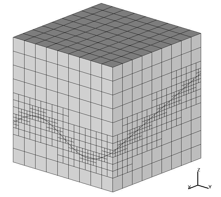
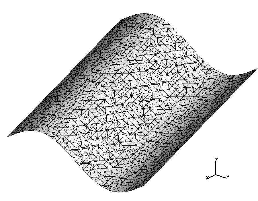
a) b) c)

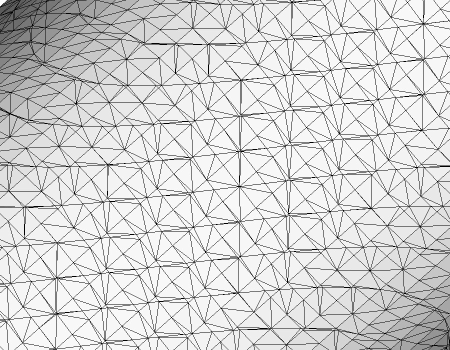
Figure 2: a) Example of a bulk domain with a fracture. In this example, the background mesh is refined near the fracture; b) The reconstructed $\Gamma_{h}$; c) The zoom-in of the induced surface triangulation $\mathcal{F}_{h}$.

Note that $\widetilde{\Gamma}_{h}$ is still not completely suitable for our purposes, since $\phi_{h}$ is trilinear and so numerical integration over its zero level is not straightforward. Therefore, we next build a suitable polygonal approximation of $\widetilde{\Gamma}_{h}$ which is our final $\Gamma_{h}$. Once $\phi_{h}$ is computed, we recover $\Gamma_{h}$ by the cubical marching squares method from [27] (a variant of the very well-known marching cubes method). The method provides a triangulation of $\widetilde{\Gamma}_{h}$ within each cube such that $\Gamma_{h}$ is continuous over cubes interfaces, the number of triangles within each cube is finite and bounded by a constant independent of $\widetilde{\Gamma}_{h}$ and a number of refinement levels. Moreover, the vertices of triangles from $\mathcal{F}_{h}$ are lying on $\widetilde{\Gamma}_{h}$. This final discrete surface $\Gamma_{h}$ is still an approximation of $\Gamma$ in the sense of (11). A example of bulk domain with embedded surface and background mesh is illustrated in Figure 2.

Note that the resulting triangulation $\mathcal{F}_{h}$ is not necessarily regular, i.e. elements from $T$ may have very small internal angles and the size of neighboring triangles can vary strongly. Thus, $\Gamma_{h}$ is not a regular triangulation of $\Gamma$. The surface triangulation $\mathcal{F}_{h}$ is used only to define quadratures in the finite element method, while approximation properties of the method depend on the volumetric octree mesh.

3.3 Monotone finite volume method

First we consider a FV method for the advection-diffusion equation (1) in each subdomain $\Omega_{i,h}$. Let $\mathcal{T}_{i,h}$ be the tessellation of $\Omega_{i,h}$ into non-intersected polyhedra, which is induced by overlapping $\Omega_{i,h}$ and the background mesh $\mathcal{T}_{h}$. Since the background mesh is the octree Cartesian, each element $T\in\mathcal{T}_{i,h}$ is either a cube, if it lies in the interior of $\Omega_{i,h}$, or a cut cube, if ${\partial\Omega}_{i,h}$ intersects a background cell from $\mathcal{T}_{h}$. We assume the octree grid is gradely refined, i.e. the sizes of two neighbouring elements of $\mathcal{T}_{h}$ can differ at most by a factor of two. Such octree grids are also known as balanced. The method applies for unbalanced octrees, but in our experiments we use balanced grids. For the balanced grid, each interior cell may have from 6 to 24 neighboring cells (cells sharing a face). In the FV method we treat such cells as a polyhedra with up to 24 faces. Since we reconstruct $\Gamma$ inside each cell as a triangulated surface without holes, the cut cell from $\mathcal{T}_{i,h}$ can be treated as a general polyhedral element as well. By $\mathcal{F}_{i,h}$ we denote the set of all faces of polyhedra from $\mathcal{T}_{i,h}$.

The FV discretization below is applied to each subdomain $\Omega_{i}$ separately, so we will skip in this section the redundant index $i$ for the concentration, coefficients and the flow vector field in $\Omega_{i}$. Note that ${\partial\Omega}_{i,D}$ includes the fracture part of the boundary of ${\partial\Omega}_{i}$.

As the first step, we assume a time discretization (say, the implicit Euler method) and consider the mixed form of (1) and boundary conditions

$$\begin{array}[]{rclll}\mathbf{q}=\mathbf{w}u-D\nabla u,\quad\tilde{\phi}\,u+\mbox{\rm div }\mathbf{q}&=&f&\mbox{~{}in}&\Omega_{i},\\ u&=&\tilde{u}_{D}&\mbox{~{}on}&{\partial\Omega}_{i,D},\\ -D\mathbf{n}_{\partial\Omega}\cdot\nabla u&=&0&\text{~{}on}&{\partial\Omega}_{i,N},\end{array}$$ (12)

where the right hand side $f$ accounts for the source term and for the values of concentration from the previous time step, $\tilde{\phi}$ is the porosity coefficient scaled by the reciprocal of the time step size, and ${\partial\Omega}_{i,D}$ includes ${\partial\Omega}_{i}\cap\Gamma$, where $\tilde{u}_{D}=v$.

For a cell $T\in\mathcal{T}_{i,h}$, $\mathbf{x}_{T}$ denotes the barycenter of $T$, and $u_{T}$ denotes the averaged concentration. We formally assign $u_{T}$ to $\mathbf{x}_{T}$. Integrating the mass balance equation (12) over $T$ and using the divergence theorem, we obtain:

$$\tilde{\phi}|T|u_{T}+\sum\limits_{\mathcal{F}\in\partial T}\mathbf{q}_{\mathcal{F}}\cdot\mathbf{n}_{\mathcal{F}}=\int_{T}f\,{\rm d}x,\qquad\mathbf{q}_{\mathcal{F}}=\frac{1}{|\mathcal{F}|}\int_{\mathcal{F}}\mathbf{q}\,{\rm d}s,$$ (13)

where $\mathbf{q}_{\mathcal{F}}\cdot\mathbf{n}_{\mathcal{F}}$ is the averaged normal flux across face $\mathcal{F}$, and $\mathbf{n}_{\mathcal{F}}$ is the normal vector on $\mathcal{F}$ pointing outward for $T$; $|\mathcal{F}|$ ($|T|$) denotes the area (volume) of $\mathcal{F}$ ($T$). The Dirichlet boundary data on faces $\mathcal{F}\in\partial\Omega_{D}$ will be accounted in the scheme via boundary faces concentration values $u_{\mathcal{F}}=\frac{1}{|\mathcal{F}|}\int_{\mathcal{F}}u_{D}\,{\rm d}s$. We assume that $u_{\mathcal{F}}$ are assigned to barycenters of faces. Enforcing homogeneous Neumann boundary conditions on faces from ${\partial\Omega}_{i,N}$ is straightforward, for $\mathcal{F}\in\partial T\cap{\partial\Omega}_{N}$ the normal flux $\mathbf{q}_{\mathcal{F}}\cdot\mathbf{n}_{\mathcal{F}}$ in (13) is set to 0.

In the conventional cell-centered FV method, the normal flux $\mathbf{q}_{\mathcal{F}}\cdot\mathbf{n}_{\mathcal{F}}$ is replaced by its discrete counterpart $\mathbf{q}_{\mathcal{F},h}\cdot\mathbf{n}_{\mathcal{F}}$, which is computed from cell concentrations $u_{T}$ and boundary data $u_{\mathcal{F}}$. For simplicity of presentation we shall omit subscript $h$ in notations of the discrete flux. The discrete flux is the combination of the diffusive and convective fluxes and we discretize them separately following [34, 35, 40].

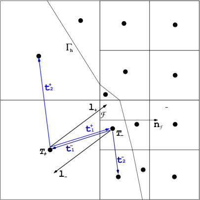
Figure 3: For the 2D case, the figure illustrates our constructions for the approximation of the directional derivative $\mathbf{l}_{\mathcal{F}}\cdot\nabla u$ on the face (edge in 2D) $\mathcal{F}=\overline{T_{+}}\cap\overline{T_{-}}$. Bold dots show the barycenters $\mathbf{x}_{T}$ of the cells from $\mathcal{T}_{1,h}$ and $\mathcal{T}_{2,h}$. The mean values of the concentration are assigned to these barycenters.

For $T\in\mathcal{T}_{i,h}$, we define $\omega(T):=\{T^{\prime}\in\mathcal{T}_{i,h}\,|\,\mbox{area}(\overline{T}^{\prime}\cap\overline{T})\neq 0\}$, the set of all neighboring cells of $T$, and $\omega_{\partial}(T):=\{F\in\mathcal{F}_{i,h}\,|\,F{\subset}\partial T\cap\partial\Omega_{i,D}\}$, the set all faces of $T$ with prescribed Dirichlet data. For $T\in\mathcal{T}_{i,h}$, the set of points $\mathcal{P}$ collects all barycenters of the elements from $\omega(T)$ and $\omega_{\partial}(T)$. Furthermore, for each $T\in\mathcal{T}_{i,h}$ we define the bundle of vectors, $\mathbf{v}(T):=\{\mathbf{t}\in\mathbb{R}^{3}\,|\,\mathbf{t}=\mathbf{y}-\mathbf{x}_{T},~{}\mathbf{y}\in\mathcal{P}(T)\}$.

Consider an arbitrary internal face $\mathcal{F}$ shared by two cells $T_{+},T_{-}$ from $\mathcal{T}_{i,h}$ and assume that $\mathbf{n}_{\mathcal{F}}$ points from $T_{+}$ to $T_{-}$. We introduce the co-normal vector $\mathbf{l}_{\mathcal{F}}=D\mathbf{n}_{\mathcal{F}}$. Vector $\mathbf{l}_{\mathcal{F}}$ can make a nonzero angle with $\mathbf{n}_{\mathcal{F}}$ in the case of an anisotropic diffusion tensor. To define the discrete diffusive flux on $\mathcal{F}$, we first consider three vectors $\mathbf{t}_{i}^{+}\in\mathbf{v}(T_{+})$, $i=1,2,3$, such that for the co-normal vector $\mathbf{l}_{\mathcal{F}}=D\mathbf{n}_{f}$ we have

$$\mathbf{l}_{\mathcal{F}}=\alpha_{+}~{}\mathbf{t}_{1}^{+}+\beta_{+}~{}\mathbf{t}_{2}^{+}+\gamma_{+}~{}\mathbf{t}_{3}^{+},$$ (14)

with non-negative coefficients $\alpha_{+}$, $\beta_{+}$ and $\gamma_{+}$. Such a triplet can be always found, (in some rare pathological situations, one has to expand $\mathcal{P}(T_{+})$ slightly, cf. [13]).

The normal flux is the directional derivative along the co-normal vector $\mathbf{l}_{+}:=\mathbf{l}_{\mathcal{F}}$, and hence it can also be represented as the linear combination of three derivatives along $\mathbf{t}_{i}^{+}$. The latter are approximated by central differences (may reduce to one side differences near Dirichlet boundaries). Thus, we get $\mathbf{q}_{\mathcal{F}}\cdot\mathbf{n}_{F}\approx q_{+}$,

$$q_{+}=\alpha^{\prime}_{+}~{}(u_{+}-u_{+,1})+\beta^{\prime}_{+}~{}(u_{+}-u_{+,2})+\gamma^{\prime}_{+}~{}(u_{+}-u_{+,3}),\qquad u_{+}=u(\mathbf{x}_{T_{+}}),~{}u_{+,i}=u(\mathbf{x}_{T_{+}}+\mathbf{t}_{i}^{+}),$$ (15)

where coefficients $\alpha^{\prime}_{+},\beta^{\prime}_{+},\gamma^{\prime}_{+}$ are computed from $\alpha$, $\beta$, $\gamma$ in (14) for the cell $T_{+}$, using the simple scaling with $|\mathbf{t}_{i}^{+}|/|\mathbf{l}_{\mathcal{F}}|$. For the same co-normal vector one has another decomposition based on $\mathbf{v}(T_{-})$ vector bundle, $\mathbf{l}_{-}:=-\mathbf{l}_{\mathcal{F}}=\alpha_{-}~{}\mathbf{t}_{1}^{-}+\beta_{-}~{}\mathbf{t}_{2}^{-}+\gamma_{-}~{}\mathbf{t}_{3}^{-}$, $\mathbf{t}_{i}^{-}\in\mathbf{v}(T_{-})$. This decomposition yields another approximation, $\mathbf{q}_{\mathcal{F}}\cdot\mathbf{n}_{F}\approx q_{-}$:

$$q_{-}=\alpha^{\prime}_{-}~{}(u_{-}-u_{-,1})+\beta^{\prime}_{-}~{}(u_{-}-u_{-,2})+\gamma^{\prime}_{-}~{}(u_{-}-u_{-,3}),\qquad u_{-}=u(\mathbf{x}_{T_{-}}),~{}u_{-,i}=u(\mathbf{x}_{T_{-}}+\mathbf{t}_{i}^{-}),$$ (16)

with non-negative coefficients $\alpha^{\prime}_{-}$, $\beta^{\prime}_{-}$ and $\gamma^{\prime}_{-}$. Figure 3 illustrates the construction in 2D.

Now we can take a linear combination of (15) and (16) with non-negative coefficients $\mu_{+}$ and $\mu_{-}$:

$$\mathbf{q}_{\mathcal{F}}\cdot\mathbf{n}_{\mathcal{F}}=\mu_{+}q_{+}+\mu_{-}(-q_{-}).$$ (17)

The discrete flux (17) approximates the differential one if $\mu_{+}$, $\mu_{-}$ satisfy

$$\mu_{+}+\mu_{-}=1.$$ (18)

Following [35], to construct the monotone FV discretization, we set both representations of the flux equal:

$$\mu_{+}q_{+}=-\mu_{-}q_{-}.$$ (19)

If $|q_{+}|=|q_{-}|=0$, then the solution of (18),(19) in not unique. In this case we choose $\mu_{+}=\mu_{-}=1/2$. Otherwise, the solution is given by

$$\mu_{+}=\frac{q_{-}}{q_{-}-q_{+}},\qquad\mu_{-}=\frac{q_{+}}{q_{+}-q_{-}}.$$

If $q_{+}q_{-}>0$, we avoid potentially degenerate case by applying the modification from [49]; see also formulas in [35], p. 374. We note that the resulting multi-point flux approximation is nonlinear and compact, i.e. the stencil includes the values of concentration only from neighboring cells.

To define the normal component of the discrete advective flux $\mathbf{q}_{\mathcal{F},a}=\frac{1}{|\mathcal{F}|}\int_{\mathcal{F}}u\mathbf{w}\,{\rm d}s$, we adopt the nonlinear upwind approximation (subscript $h$ is again omitted for the sake of notation):

$$\mathbf{q}_{\mathcal{F},a}\cdot\mathbf{n}_{\mathcal{F}}=w_{\mathcal{F}}^{+}\mathcal{R}_{T^{+}}(\mathbf{x}_{\mathcal{F}})+w_{\mathcal{F}}^{-}\mathcal{R}_{T^{-}}(\mathbf{x}_{\mathcal{F}}),$$ (20)

where

$$w_{\mathcal{F}}^{+}=\frac{1}{2}(w_{\mathcal{F}}+|w_{\mathcal{F}}|),\quad w_{\mathcal{F}}^{-}=\frac{1}{2}(w_{\mathcal{F}}-|w_{\mathcal{F}}|),\quad w_{\mathcal{F}}=\frac{1}{|\mathcal{F}|}\int_{\mathcal{F}}\mathbf{w}\cdot\mathbf{n}_{\mathcal{F}}\,{\rm d}s,$$

$\mathcal{R}_{T}$ is a linear reconstruction of the concentration over cell $T$ which depends on the concentration values from neighboring cells.

On each cell $T$, the linear reconstruction is defined by

$$\mathcal{R}_{T}(\mathbf{x})=\left\{\begin{array}[]{ll}u_{T}+\mathcal{L}_{T}\mathbf{g}_{T}\cdot(\mathbf{x}-\mathbf{x}_{T}),&\mathbf{x}\in T,\\ 0,&\mathbf{x}\notin T,\end{array}\right.$$ (21)

where $\mathbf{g}_{T}$ denotes the gradient of the linear reconstruction of concentration in $\mathbf{x}_{T}$, and $\mathcal{L}_{T}$ is a slope limiting operator. The gradient is recovered from the best affine least-square fit for $u_{h}$ over a subset of barycenter nodes and, possibly, the boundary data nodes from cells neighboring $T$. The slope limiting operator $\mathcal{L}_{T}$ is introduced to avoid non-physical extrema. It provides the smallest possible changes of the reconstructed least-square slope. Details can be found in [34, 35, 40].

Replacing fluxes in equations (13) by their numerical approximations, we obtain a system of nonlinear equations

$$\Phi\mathbf{U}+\mathbf{M}(\mathbf{U})\,\mathbf{U}=\mathbf{F}(\mathbf{U}),\qquad\mathbf{M}(\mathbf{U})=\mathbf{M}_{dif}(\mathbf{U})+\mathbf{M}_{adv}(\mathbf{U}),$$ (22)

with a diagonal matrix $\Phi$. For any fixed vector $\mathbf{V}$, $\mathbf{M}(\mathbf{V})$ is a square sparse matrix, $\mathbf{F}(\mathbf{V})$ is a right-hand side vector. Matrix $\mathbf{M}_{dif}$ is an M-matrix which has diagonal dominance in rows. The stencil of this matrix is compact, each row contains non-zero off-diagonal entries corresponding mainly (and in most cases only) to degrees of freedom at the cells sharing a face with the current cell. For a cubic uniform mesh and the Poisson equation, the matrix $\mathbf{M}_{dif}$ corresponds to the conventional seven-point stencil. Although matrix $\mathbf{M}_{adv}$ has no diagonal dominance in rows, it can be shown, cf. [35], that the solution to (22) satisfies the discrete maximum principle.

3.4 The trace finite element method

Consider now the volumetric finite element space of all piecewise trilinear continuous functions with respect to the bulk octree mesh $\mathcal{T}_{h}$:

$$V_{h}:=\{v_{h}\in C(\Omega)\ |\ v|_{S}\in Q_{1}~{}~{}\forall\ S\in\mathcal{T}_{h}\},\quad\text{with}~{}~{}Q_{1}=\mbox{span}\{1,x_{1},x_{2},x_{3},x_{1}x_{2},x_{1}x_{3},x_{2}x_{3},x_{1}x_{2}x_{3}\}.$$ (23)

The surface finite element space is the space of traces on $\Gamma_{h}$ of all piecewise trilinear continuous functions with respect to the outer triangulation $\mathcal{T}_{h}$ defined as follows

$$V_{h}^{\Gamma}:=\{\psi_{h}\in H^{1}(\Gamma_{h})\ |\ \exists~{}v_{h}\in V_{h}\ \text{such that }\ \psi_{h}=v_{h}|_{\Gamma_{h}}\}.$$ (24)

Given the surface finite element space $V_{h}^{\Gamma}$, the finite element discretization of (2) is as follows: Find $v_{h}\in V_{h}^{\Gamma}$ such that $v_{h}|_{\partial\Gamma_{D,h}}=v_{D}^{h}$ and

$$\int_{\Gamma_{h}}\left(\phi_{\Gamma,h}\frac{\partial v_{h}}{\partial t}w_{h}+d_{h}D_{\Gamma,h}\nabla_{\Gamma_{h}}v_{h}\cdot\nabla_{\Gamma_{h}}w_{h}\,+(\mathbf{w}_{h}\cdot\nabla_{\Gamma_{h}}v_{h})w_{h}\right)\,+(\mbox{\rm div}_{\Gamma_{h}}\mathbf{w}_{h})\,{w_{h}}v_{h}\mathrm{d}\mathbf{s}_{h}\\ =\int_{\Gamma_{h}}(F_{\Gamma,h}(u_{h})+f_{\Gamma,h})w_{h}\,\mathrm{d}\mathbf{s}_{h}$$ (25)

for all $w_{h}\in V_{h}^{\Gamma}$, s.t. $w_{h}|_{\partial\Gamma_{D,h}}=0$ . Here $\mathbf{w}_{h}$, $v_{D}^{h}$, $d_{h}$, $D_{\Gamma,h}$ and $f_{\Gamma,h}$ are the problem data lifted from $\Gamma$ to $\Gamma_{h}$, in the case if $\Gamma\neq\Gamma_{h}$. The bulk domain contributes through the flux $F_{\Gamma,h}(u_{h})$, which is reconstructed from the numerical concentration in the porous matrix.

Similar to the plain Galerkin finite element for advection-diffusion equations the method (25) is prone to instability unless mesh is sufficiently fine such that the mesh Peclet number is less than one. Following [42], we consider the SUPG stabilized TraceFEM. The stabilized formulation reads: Find $v_{h}\in V_{h}^{\Gamma}$ such that

$$\int_{\Gamma_{h}}\left(\phi_{\Gamma,h}\frac{\partial v_{h}}{\partial t}w_{h}+d_{h}D_{\Gamma,h}\nabla_{\Gamma_{h}}v_{h}\cdot\nabla_{\Gamma_{h}}w_{h}\,+(\mathbf{w}_{h}\cdot\nabla_{\Gamma_{h}}v_{h})w_{h}\right)\,+(\mbox{\rm div}_{\Gamma_{h}}\mathbf{w}_{h})\,{w_{h}}v_{h}\mathrm{d}\mathbf{s}_{h}\\ +\sum_{{T}\in\mathcal{F}_{h}}\delta_{K}\int_{K}(\phi_{\Gamma,h}\frac{\partial v_{h}}{\partial t}-{d_{h}\mbox{\rm div}_{\Gamma_{h}}D_{\Gamma,h}\nabla_{\Gamma_{h}}}v_{h}+\mathbf{w}_{h}\cdot\nabla_{\Gamma_{h}}v_{h}+(\mbox{\rm div}_{\Gamma_{h}}\mathbf{w}_{h})\,v_{h})\,\mathbf{w}_{h}\cdot\nabla_{\Gamma_{h}}w_{h}\,\mathrm{d}\mathbf{s}_{h}\\ =\int_{\Gamma_{h}}(F_{\Gamma,h}(u_{h})+f_{\Gamma,h})w_{h}\,\mathrm{d}\mathbf{s}_{h}+\sum_{K\in\mathcal{F}_{h}}\delta_{K}\int_{K}(F_{\Gamma,h}(u_{h})+f_{\Gamma,h})(\mathbf{w}_{h}\cdot\nabla_{\Gamma_{h}}w_{h})\,\mathrm{d}\mathbf{s}_{h}\quad\forall~{}w_{h}\in V_{h}^{\Gamma}.$$ (26)

For the definition of $K\in\mathcal{F}_{h}$, $T_{K}\in\mathcal{T}_{h}$ we refer to section 3.2. The stabilization parameter $\delta_{K}$ depends on $K\subset T_{K}$. The side length of the cubic cell $T_{K}$ is denoted by $h_{T_{K}}$. Let $\displaystyle\mathsf{Pe}_{K}:=\frac{h_{T_{K}}\|\mathbf{w}_{h}\|_{L^{\infty}(K)}}{2\varepsilon}$ be the cell Peclet number. We take

$${\delta_{K}}=\left\{\begin{aligned} &\frac{\delta_{0}h_{T_{K}}}{\|\mathbf{w}_{h}\|_{L^{\infty}(K)}}&&\quad\hbox{ if }\mathsf{Pe}_{K}>1,\\ &\frac{\delta_{1}h^{2}_{T_{K}}}{\varepsilon}&&\quad\hbox{ if }\mathsf{Pe}_{K}\leq 1,\end{aligned}\right.$$ (27)

with some given positive constants $\delta_{0},\delta_{1}\geq 0$.

For the matrix–vector representation of the TraceFEM one uses the nodal basis of the bulk finite element space $V_{h}$ rather than tries to construct a basis in $V_{h}^{\Gamma}$. This convenient choice, however, has some consequences. In general, the restrictions to $\Gamma_{h}$ of the outer nodal basis functions on $\Gamma_{h}$ can be linear dependent or (in most cases) almost linear dependent. This and small cuts of background cells lead to badly conditioned mass and stiffness matrices. In recent years stabilizations have been developed which are easy to implement and result in matrices with acceptable condition numbers, see the overview in [44]. In this paper we use the “full gradient” stabilization of the TraceFEM [15, 48]. In this variant of the method, one modifies the surface diffusion part of the method (25) to include the normal part of the gradient:

$$\int_{\Gamma_{h}}d_{h}D_{\Gamma,h}\nabla_{\Gamma_{h}}v_{h}\cdot\nabla_{\Gamma_{h}}w_{h}\,\mathrm{d}\mathbf{s}_{h}\quad\text{yields to}\quad\int_{\Gamma_{h}}d_{h}D_{\Gamma,h}\nabla v_{h}\cdot\nabla w_{h}\,\mathrm{d}\mathbf{s}_{h}.$$

We note that the method remains consistent on smooth surfaces (up to second order geometric errors), since the true surface solution extended off the surface along normal directions satisfies both variational formulations on $\Gamma$. The modification improves algebraic properties of the (diagonally scaled) stiffness matrix of the method [48]. The full-gradient method uses the background finite element space $V_{h}$ instead of the surface finite element space $V_{h}^{\Gamma}$ in (25). However, practical implementation of both methods uses the frame of all bulk finite element nodal basis functions $\phi_{i}\in V_{h}$ such that $\mbox{supp}(\phi_{i})\cap\Gamma_{h}\neq\emptyset$. Hence the active degrees of freedom in both methods are the same. The stiffness matrices are, however, different.

3.5 Coupling between discrete bulk and surface equations

The equations in the bulk and on the surface are coupled through the boundary condition $u_{i}=v$ on $\partial\Omega_{i,h}\cap\Gamma_{h}$ (second equation in (1)) and the net flux $F_{\Gamma_{h}}(u)$ on $\Gamma_{h}$, which stands as the source term in the surface equation (2). On $\Gamma_{h}$ the solution $v_{h}$ is defined as a trace of the background finite element piecewise trilinear function. The averaged value of $v_{h}$ is computed on each surface triangle $K\in\mathcal{F}_{h}$ using a standard quadrature rule. These values assigned to the barycenters of $K$ from $\mathcal{F}_{h}$ serve as the Dirichlet boundary data for the FV method on $\Gamma_{h}$. The discrete diffusive and convective fluxes are assigned to barycenters of all faces on $\mathcal{T}_{i,h}$, $i=1,\dots,N$. Since each triangle $K\in\mathcal{F}_{h}$ is a face for two cells $T_{i}\in\mathcal{T}_{i,h}$ and $T_{j}\in\mathcal{T}_{j,h}$, $i\neq j$, the diffusive and convective fluxes are assigned to $K$ from both sides of $\Gamma_{h}$. The discrete net flux $F_{\Gamma_{h}}(u_{h})$ at the barycenter of $K$ is computed as the jump of the fluxes over $K$. In the TraceFEM this value is assigned to all $\mathbf{x}\in K$, and numerical integration is done over all surface elements $K\in\mathcal{F}_{h}$ to compute the right-hand side of the algebraic system.

To satisfy all (discretized) equations and boundary conditions we iterate between the bulk FV and surface FE solvers on each time step. We assume an implicit time stepping method (in experiments we use backward Euler). This results in the following system on each time step.

$$\left\{\begin{aligned} \mathcal{L}u:=\tilde{\phi}u+\mbox{\rm div}(\mathbf{w}u-D\nabla)u&=\hat{f}\quad\text{in}~{}\Omega\setminus\Gamma,\\ u&=v\quad\text{on}~{}\Gamma,\\ {D}\mathbf{n}_{\partial\Omega}\cdot\nabla u=0\quad\text{on}~{}{\partial\Omega}_{N},\quad u&=u_{D}\quad\text{on}~{}{\partial\Omega}_{D},\\ \mathcal{L}_{\Gamma}v:=\tilde{\phi}_{\Gamma}v+\mbox{\rm div}_{\Gamma}(\mathbf{w}_{\Gamma}v-dD_{\Gamma}\nabla_{\Gamma}v)&=F_{\Gamma}(u)+\hat{f}_{\Gamma}\quad\text{on}~{}~{}\Gamma,\\ {D}_{\Gamma}\mathbf{n}_{\partial\Gamma}\cdot\nabla v=0\quad\text{on}~{}{\partial\Gamma}_{N},\quad v&=v_{D}\quad\text{on}~{}{\partial\Gamma}_{D},\end{aligned}\right.$$ (28)

the right hand sides $\hat{f}$ and $\hat{f}_{\Gamma}$ account for the solution values at the previous time step. Note that condition (5) is satisfied by the construction of trace spaces in the finite element method and condition (6) is accounted weakly by the TraceFEM variational formulation.

We solve the coupled system (28) by the fixed point method: Given ${u}^{0},{v}^{0}$, the initial guess, we iterate for $k=0,1,2,\dots$ until convergence:
Step 1: Solve for ${u}^{k+1}$,

$$\left\{\begin{aligned} \mathcal{L}{u}^{k+1}&=\hat{f}~{}\text{in}~{}\Omega\setminus\Gamma,\quad{u}^{k+1}={v}^{k}\quad\text{on}~{}\Gamma,\\ {D}\mathbf{n}_{\partial\Omega}\cdot\nabla{u}^{k+1}&=0\quad\text{on}~{}{\partial\Omega}_{N},\quad{u}^{k+1}=u_{D}\quad\text{on}~{}{\partial\Omega}_{D},\\ \end{aligned}\right.$$ (29)

Step 2: Solve for ${v}^{\rm aux}$ and update for ${v}^{k+1}$ with a relaxation parameter $\omega$,

$$\left\{\begin{aligned} \mathcal{L}_{\Gamma}{v}^{\rm aux}&=F_{\Gamma}(u^{k+1})+\hat{f}_{\Gamma}\quad\text{on}~{}~{}\Gamma,\\ {D}_{\Gamma}\mathbf{n}_{\partial\Gamma}\cdot\nabla_{\Gamma}{v}^{\rm aux}&=0\quad\text{on}~{}{\partial\Gamma}_{N},\quad{v}^{\rm aux}=v_{D}\quad\text{on}~{}{\partial\Gamma}_{D}\\ {v}^{k+1}&=\omega{v}^{\rm aux}+(1-\omega){v}^{k},\quad\omega\in(0,1],\end{aligned}\right.$$ (30)

Remark 3.1.

Below we show that the fixed point method is equivalent to a preconditioned Richardson iteration for the discrete Poincaré–Steklov operator. Assume that $\mathcal{L}$ is linear (this is true for our differential model, but the particular FV discretization applied here is actually non-linear). Let’s split $u=u_{0}+\hat{u}$, $v=v_{0}+\hat{v}$, where $u_{0},\,v_{0}$ satisfy

$$\left\{\begin{aligned} \mathcal{L}u_{0}&=\hat{f}~{}\text{in}~{}\Omega\setminus\Gamma,\quad u_{0}=0\quad\text{on}~{}\Gamma,\\ D\mathbf{n}_{\partial\Omega}\cdot\nabla u_{0}&=0\quad\text{on}~{}{\partial\Omega}_{N},\quad u_{0}=u_{D}\quad\text{on}~{}{\partial\Omega}_{D},\end{aligned}\right.\qquad\left\{\begin{aligned} \mathcal{L}_{\Gamma}{v}_{0}&=0\quad\text{on}~{}~{}\Gamma,\\ D_{\Gamma}\mathbf{n}_{\partial\Gamma}\cdot\nabla{v}_{0}&=0\quad\text{on}~{}{\partial\Gamma}_{N},\quad{v}_{0}=v_{D}\quad\text{on}~{}{\partial\Gamma}_{D}\end{aligned}\right.$$

Now the iterations (29)–(30) can be written in terms of $\hat{u}$ and $\hat{v}$ parts of the bulk and surface concentrations:

$$\begin{split}\left\{\begin{aligned} \mathcal{L}\hat{u}^{k+1}&=0~{}\text{in}~{}\Omega\setminus\Gamma,\quad\hat{u}^{k+1}=\hat{v}^{k}\quad\text{on}~{}\Gamma,\\ {D}\mathbf{n}_{\partial\Omega}\cdot\nabla\hat{u}^{k+1}&=0\quad\text{on}~{}{\partial\Omega}_{N},\quad\hat{u}^{k+1}=0\quad\text{on}~{}{\partial\Omega}_{D},\\ \end{aligned}\right.\\ \left\{\begin{aligned} \mathcal{L}_{\Gamma}\hat{v}^{\rm aux}&=F_{\Gamma}(u^{k+1})+\hat{f}_{\Gamma}\quad\text{on}~{}~{}\Gamma,\\ {D}_{\Gamma}\mathbf{n}_{\partial\Gamma}\cdot\nabla_{\Gamma}\hat{v}^{\rm aux}&=0\quad\text{on}~{}{\partial\Gamma}_{N},\quad\hat{v}^{\rm aux}=0\quad\text{on}~{}{\partial\Gamma}_{D}\\ \hat{v}^{k+1}&=\omega\hat{v}^{\rm aux}+(1-\omega)\hat{v}^{k},\quad\omega\in(0,1].\end{aligned}\right.\end{split}$$ (31)

Now we note that $\hat{u}$ is a (generalized) harmonic extension of $\hat{v}$ on $\Omega\setminus\Gamma$ and $S_{\Gamma}\,:\,\hat{v}\to F_{\Gamma}(\hat{u})$ is the Dirichlet to Neumann (discrete) Poincaré–Steklov operator. Using this notation, one can write the surface equation for $\hat{v}$ in the compact operator form,

$$(\mathcal{L}_{\Gamma,0}-S_{\Gamma})\hat{v}=\hat{F}\quad\text{on}~{}~{}\Gamma,\quad\text{with}~{}~{}\hat{F}:=F_{\Gamma}(u_{0})+\hat{f}_{\Gamma}.$$ (32)

We use zero index in $\mathcal{L}_{\Gamma,0}$ to stress that the operator accounts for homogenous boundary conditions on ${\partial\Gamma}$. It is easy to see that (31) is the Richardson iterative process for the surface equation (32), with the preconditioner $W=\mathcal{L}_{\Gamma,0}^{-1}$ and the relaxation parameter $\omega$:

$$\hat{v}^{k+1}=\hat{v}^{k}-\omega\,W\left(\,(\mathcal{L}_{\Gamma}-S_{\Gamma})\hat{v}^{k}-\hat{F}\right),\quad k=0,1,2,\dots.$$ (33)

From (33) we see that a more efficient iterative process based on a different choice of preconditioner and employing Krylov subspaces may be feasible (if $\mathcal{L}$ is non-linear one may consider Anderson’s mixing to accelerate convergence). However, we do not pursue this topic further in this paper.

4 Numerical results and discussion

This section collects several numerical examples, which demonstrate the accuracy and capability of the hybrid method. We perform a series of tests, where we simulate steady and time-dependent solutions in a bulk domain with an imbedded fracture. We also include an a example with a smooth curved surface (a sphere) embedded in a bulk domain and a given analytical solution for a surface-bulk problem with Henry interface condition. To measure the error we shall use $L^{2}$, $H^{1}$ and $L^{\infty}$ surface and volume norms. For the computed solutions $u_{h},v_{h}$ and true solutions $u,v$, these norms are defined below. In the volume, we set

$$\begin{split}&\mbox{err}_{L^{\infty}(\Omega)}:=\max_{T\in\mathcal{T}_{h}}|u_{h}(\mathbf{x}_{T})-u(\mathbf{x}_{T})|,\quad\mbox{err}_{L^{2}(\Omega)}:=\left(\sum_{T\in\mathcal{T}_{h}}\text{vol}(T)|u_{h}(\mathbf{x}_{T})-u(\mathbf{x}_{T})|^{2}\right)^{\frac{1}{2}},\\ &\mbox{err}_{H^{1}(\Omega)}:=\left(\sum_{T\in\mathcal{T}_{h}}\text{vol}(T)|\nabla I(u_{h})(\mathbf{x}_{T})-\nabla u(\mathbf{x}_{T})|^{2}\right)^{\frac{1}{2}},\end{split}$$

where $I(u_{h})$ is the $P_{1}$ least-square interpolant to the values of $u_{h}$ in barycenters of the cells from $\omega(\mathbf{x}_{T})\cap\Omega_{i}$, for $T\in\Omega_{i}$. Over the surface, we set

$$\mbox{err}_{L^{\infty}(\Gamma)}:=\max_{\Gamma}|v_{h}-v^{e}|,\quad\mbox{err}_{L^{2}(\Gamma)}:=\|v_{h}-v^{e}\|_{L^{2}(\Gamma)},\quad\mbox{err}_{H^{1}(\Gamma)}:=\|\nabla_{\Gamma_{h}}v_{h}-\nabla_{\Gamma_{h}}v\|_{L^{2}(\Gamma)},$$

where $v^{e}$ is the extension of $v$ from $\Gamma$ to $\Gamma_{h}$ along normal directions to $\Gamma$.

4.1 Steady analytical solution for a triple fracture problem

Our next experiment deals with the coupled surface–bulk diffusion problem in the domain $\Omega=[0,1]^{3}$ with an embedded piecewise planar $\Gamma$. We design $\Gamma$ to model a branching fracture. In the basic model, $\Gamma=\Gamma(0)$ consists of three planar pieces,

$$\Gamma(0)=\Gamma_{12}\cup\Gamma_{13}\cup\Gamma_{23},\quad\Gamma_{ij}=\overline{\Omega_{i}}\cap\overline{\Omega_{j}}~{}~{}i\neq j,$$

such that

$$\Omega_{1}=\{\mathbf{x}\in\Omega\,|\,x<\frac{1}{2}~{}\text{and}~{}y>x\},\quad\Omega_{2}=\{\mathbf{x}\in\Omega\,|\,x>\frac{1}{2}~{}\text{and}~{}y>x-1\},\quad\Omega_{3}=\Omega\setminus(\overline{\Omega}_{1}\cup\overline{\Omega}_{2}).$$

This subdivision is illustrated in Figure 4 (left). The pieces $\Gamma_{ij}$ belong to certain planes of symmetry for the cube, and so the induced triangulation of $\Gamma(0)$ and the cut cells in the bulk domain are all quite regular. To model a generic situation when $\Gamma$ cuts through the background mesh in an arbitrary way, we consider other tessellations of $\Omega=[0,1]^{3}$ into three subdomains by a surface $\Gamma(\alpha)$. The surface $\Gamma(\alpha)$ is obtained from $\Gamma(0)$ by applying the clockwise rotation by the angle $\alpha$ around the axis $x=z=0.5$. We take $\alpha=20^{o}$ and $\alpha=40^{o}$, the resulting tessellations of $\Omega$ are illustrated in Figure 4 (middle and right pictures). More precisely, we define

$$\Gamma(\alpha)=\{\mathbf{x}\in\Omega\,|\,\mathbf{y}\in\Gamma(0),~{}\mathbf{y}-\mathbf{x}_{0}=\mathcal{Q}_{\alpha}(\mathbf{x}-\mathbf{x}_{0})\},~{}~{}\text{with}~{}\mathcal{Q}_{\alpha}=\begin{bmatrix}\cos\alpha&0&-\sin\alpha\\ 0&1&0\\ \sin\alpha&0&\cos\alpha\end{bmatrix},~{}\mathbf{x}_{0}=({\footnotesize\frac{1}{2}},0,{\footnotesize\frac{1}{2}})^{T}.$$

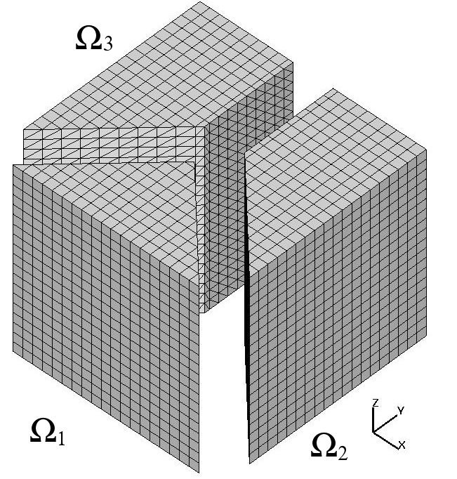
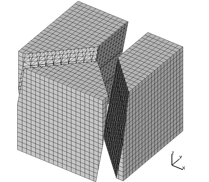
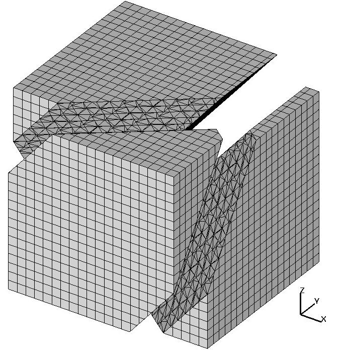
Figure 4: The figure illustrates the bulk domain with uniform mesh and the fracture. On the left picture the fracture is set orthogonal to the $xy$-plane, while on the middle and right pictures the fracture is rotated by 20 and 40 degrees.

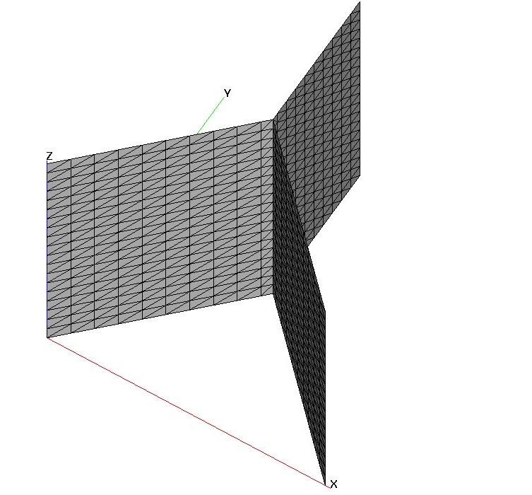
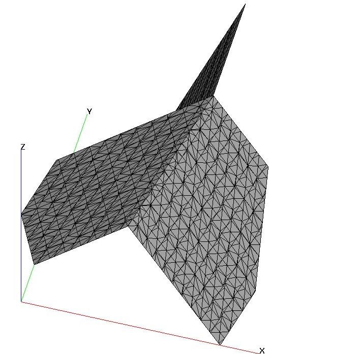
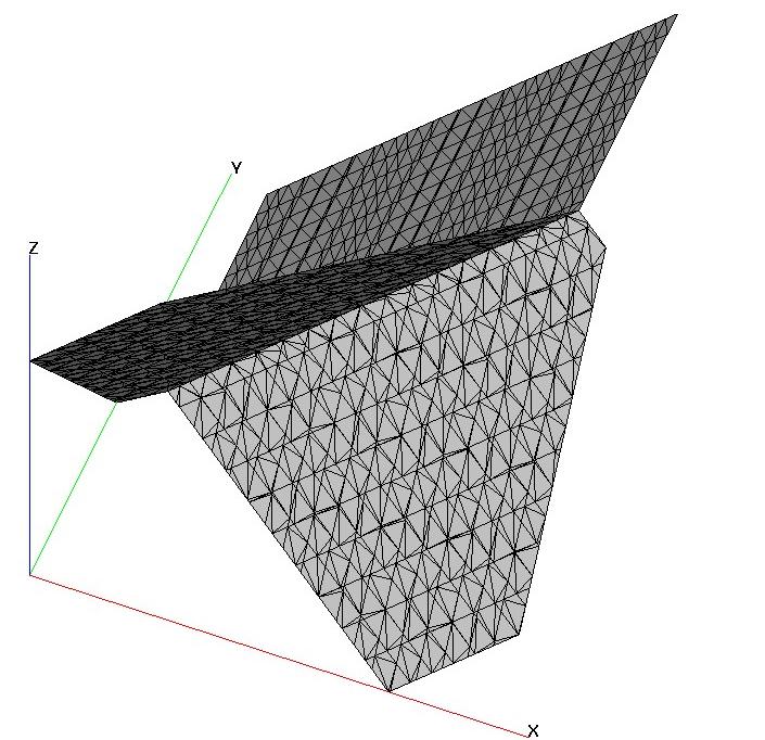
Figure 5: The figure illustrates the induced surface mesh on the fracture, when it cuts through the uniform bulk mesh in different ways.

Similar to the series of numerical experiments with the embedded spherical $\Gamma$, here we set the source terms $f_{i}$ and $f_{\Gamma}$ and the boundary conditions such that the solution to the stationary problem (1)–(7) is known. To define the solution $\{v,u\}$ solving the stationary equations (1)–(7), we first introduce

$$\psi_{1}=\left\{\begin{array}[]{lr}16(y-\frac{1}{2})^{4},&y>\frac{1}{2}\\ 0,&y\leq\frac{1}{2}\\ \end{array}\right.,\quad\psi_{2}=x-y,\quad\psi_{3}=x+y-1.$$

We define the solution of the basic model problem ($\alpha=0$)

$$u(\mathbf{x})=\left\{\begin{array}[]{rl r}&\sin(2\pi z)\cdot\psi_{2}(\mathbf{x})\cdot\phi_{3}(\mathbf{x})&\mathbf{x}\in\Omega_{1},\\ &\sin(2\pi z)\cdot\psi_{1}(\mathbf{x})&\mathbf{x}\in\Omega_{2},\\ &\sin(2\pi z)2x\cdot\psi_{1}(\mathbf{x})&\mathbf{x}\in\Omega_{3},\end{array}\right.\qquad v=u|_{\Gamma(0)}.$$

Note that the constructed exact solution is continuous across $\Gamma(0)$, but the normal derivatives are discontinuous. Other parameters in (1)–(2) are set to be $\mathbf{w}=\mathbf{w}_{\Gamma}=0$, $\phi_{1}=\phi_{2}=\phi_{\Gamma}=0$, $D_{1}=D_{2}=D_{\Gamma}=I$, and $d=1$. For the problem setup with the rotated fracture, $\alpha>0$ we set the exact solution $v_{\alpha}(\mathbf{x})=v(\mathbf{y})$, $u_{\alpha}(\mathbf{x})=u(\mathbf{y})$, with $\mathbf{y}=\mathcal{Q}_{\alpha}(\mathbf{x}-({\small\frac{1}{2}},0,{\small\frac{1}{2}})^{T})$.

Table 1: The error in the numerical solution for the steady problem with triple fracture, $\alpha=0$.

	#d.o.f.	$L^{2}$-norm	rate	$H^{1}$-norm	rate	$L^{\infty}$-norm	rate
$\Omega$	855	6.374e-3		4.214e-1		3.920e-2
	7410	1.698e-3	1.84	1.631e-1	1.36	1.276e-2	1.56
	61620	4.235e-4	1.97	6.193e-2	1.39	3.506e-3	1.83
	502440	1.044e-4	2.00	2.348e-2	1.40	1.129e-3	1.62
$\Gamma$	232	8.469e-3		2.914e-1		9.280e-3
	1242	2.003e-3	1.79	1.387e-1	0.92	2.779e-3	1.44
	5662	5.588e-4	1.84	6.874e-2	1.01	1.217e-3	1.09
	24102	1.791e-4	1.64	3.395e-2	1.02	5.181e-4	1.18

Table 2: The error in the numerical solution for the steady problem with triple fracture, $\alpha=20$.

	#d.o.f.	$L^{2}$-norm	rate	$H^{1}$-norm	rate	$L^{\infty}$-norm	rate
$\Omega$	965	6.319e-3		4.208e-1		3.754e-2
	7872	1.805e-3	1.79	1.661e-1	1.34	1.280e-2	1.55
	63592	5.623e-4	1.80	6.371e-2	1.38	3.411e-3	1.90
	510390	1.602e-4	1.81	2.442e-2	1.39	1.146e-3	1.57
$\Gamma$	321	7.792e-3		2.694e-1		2.716e-2
	1692	2.084e-3	1.59	1.240e-1	1.12	5.400e-3	1.94
	7944	7.019e-4	1.41	6.291e-2	0.98	2.001e-3	1.29
	33272	2.441e-4	1.52	3.173e-2	0.99	7.217e-4	1.47

Table 3: The error in the numerical solution for the steady problem with triple fracture, $\alpha=40$.

	#d.o.f.	$L^{2}$-norm	rate	$H^{1}$-norm	rate	$L^{\infty}$-norm	rate
$\Omega$	991	5.934e-3		4.080e-1		3.783e-2
	7996	1.700e-3	1.80	1.621e-1	1.33	1.276e-2	1.56
	64046	4.907e-4	1.80	6.263e-2	1.37	3.515e-3	1.86
	512258	1.503e-4	1.82	2.541e-2	1.39	1.237e-3	1.61
$\Gamma$	353	8.167e-3		2.709e-1		2.696e-2
	1932	2.146e-3	1.66	1.275e-1	1.09	5.566e-3	1.85
	8766	7.115e-4	1.59	6.279e-2	1.02	2.063e-3	1.31
	36676	2.538e-4	1.49	3.121e-2	1.01	7.251e-4	1.51

The numerical results for this coupled problem with the triple fracture problem are reported in Tables 1–3. We observe stable convergent results for $\alpha=0$ as well as for more general case of $\alpha>0$. An interesting feature of this problem is that the surface $\Gamma$ is only piecewise smooth. The bulk grid is not fitted to the internal edge $\mathcal{E}=\Gamma_{12}\cap\Gamma_{13}\cap\Gamma_{23}$, and hence the tangential derivatives of $v$ are discontinuous inside certain cubic cells from $\mathcal{T}_{h}^{\Gamma}$. Therefore, a kink in $v$ cannot be represented by the finite element approximation. This may result in a reduction of convergence order. Both the performance of the FV method for cut cells (cut cells inherit a regular structure from the background mesh for $\alpha=0$, but are very irregular for $\alpha>0$ ) and the presence of the kink influences the observed convergence rates.

Table 4: Iteration numbers in (29)–(30) for the steady problem example in section 4.1.

ref. level.	$\alpha=0$	$\alpha=20^{o}$	$\alpha=40^{o}$
0	22	74	24
1	29	90	32
2	212	325	228
3	782	917	851

Finally, Table 4 shows the performance of the fixed-point iteration (29)–(30). We set $\omega=1$ and take $u^{0}=0$, $v^{0}=0$. The solver is stopped after a relative reduction of the Euclidean norm of both surface and bulk equations residuals by a factor of $10^{4}$ (a stronger convergence criterion was not found to improve solution accuracy). In each outer iteration, the surface linear subproblem was solved by exact factorization, while a few Picard iterations with exact factorization of linearized problem were done to solve the bulk system in (29). The solver does not scale in an optimal way with respect to the mesh size and more research is needed to improve its performance, cf. Remark 3.1. We postpone this topic for the future research. We also note that for time dependent problems studied below including time-dependent terms and taking initial guess to be the solution from the previous time step improves convergence of (29)–(30) a lot, and we typically need 1 or 2 iterations for each time step.

4.2 Propagating front in the porous medium with triple fracture

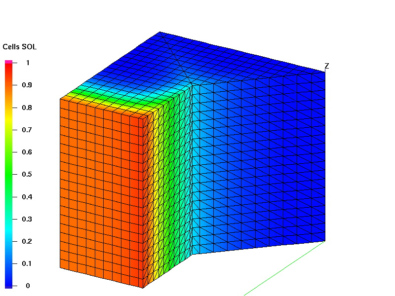
a)    b)  

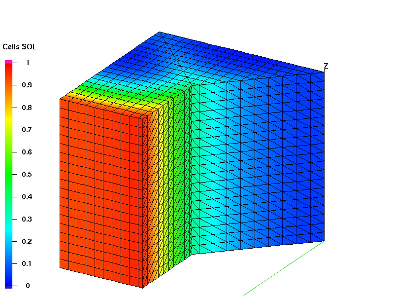
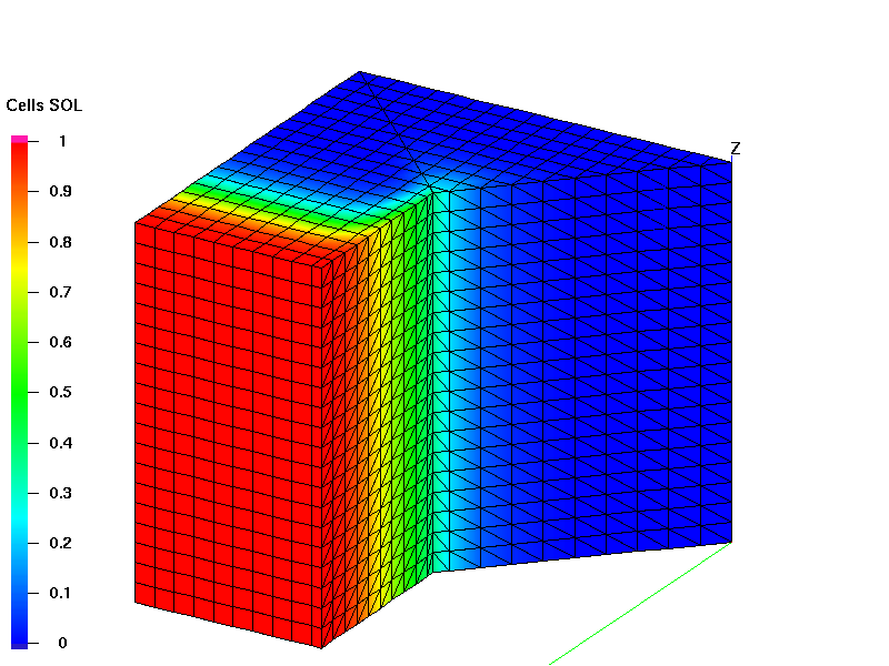
c)    d)  

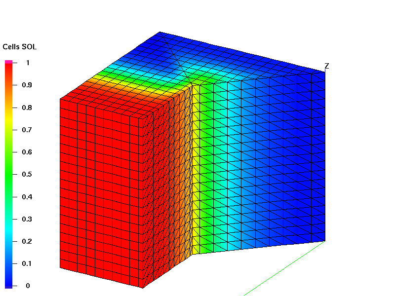
Figure 6: The figures illustrates the propagating front of the concentration in the fracture and in the bulk: Pictures a), b) show dominating diffusion case, while c), d) show dominating convection case. Pictures a) and c) show snapshots of the computed solution at time t=0.018, while pictures b) and d) snapshots the computed solution at time t=0.033. Click on picture c) to run full animation of the experiment.

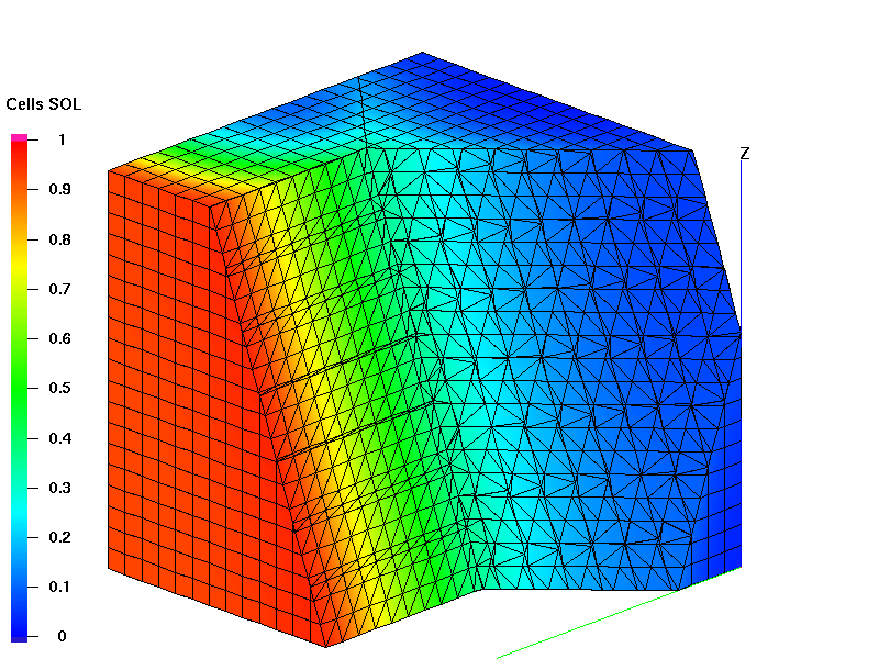
a)    b)  

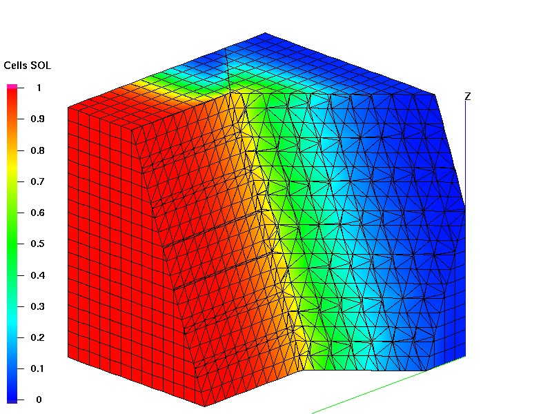
Figure 7: The figures illustrates the propagating front of the concentration in the fracture and in the bulk, with $\alpha=20^{o}$: Picture a) shows dominating diffusion case, picture b) shows dominating convection case; both at time t=0.033. Click on picture a) to run full animation of the experiment.

In the last series of experiments we compute the time dependent solution of (1)–(7). The bulk domain $\Omega$ and the fracture $\Gamma$ are the same as in the previous experiment in section 3. At time $t_{0}=0$ we set $u(t_{0})=0$ in $\Omega$ and $v(t_{0})=0$ on $\Gamma$. On the face $\{y=1\}$ of the cube we prescribe the constant concentration of a contaminant, while on other parts on the boundary the diffusion flux is set equal zero. Thus in (7), we have

$$\begin{split}\partial\Omega_{D}&=\partial\Omega\cap\{y=1\},\quad\partial\Omega_{N}=\partial\Omega\setminus\partial\Omega_{D},\quad\partial\Gamma_{D}=\partial\Gamma\cap\{y=1\},\quad\partial\Gamma_{N}=\partial\Gamma\setminus\partial\Omega_{D},\\ u_{D}&=1,\quad v_{D}=1,\quad u_{0}=0,\quad\text{and}\quad v_{0}=0.\end{split}$$

The time independent velocity field transports the contaminant in the bulk and along the fractures. We set

$$\begin{split}\mathbf{w}_{i}&=2\kappa(0,-1,0)^{T},~{}~{}i=1,2,3,\quad\text{in}~{}\Omega\\ \mathbf{w}_{\Gamma}&=5\kappa(0,-1,0)^{T}~{}~{}\quad\text{in}~{}\Gamma_{12},\quad\mathbf{w}_{\Gamma}=\kappa\mathcal{Q}_{\alpha}({\footnotesize\frac{1}{\sqrt{2}}},-{\footnotesize\frac{1}{\sqrt{2}}},0)^{T}~{}~{}\quad\text{in}~{}\Gamma_{23},\quad\mathbf{w}_{\Gamma}=\kappa\mathcal{Q}_{\alpha}(-{\footnotesize\frac{1}{\sqrt{2}}},-{\footnotesize\frac{1}{\sqrt{2}}},0)^{T}~{}~{}\quad\text{in}~{}\Gamma_{13},\end{split}$$

where $\kappa\geq 0$ is a parameter. One easily verifies the condition (4) on the edge $\mathcal{E}=\Gamma_{12}\cap\Gamma_{13}\cap\Gamma_{23}$. Other parameters are set to be

$$D_{1}=D_{2}=0.1\,I,\quad d=1,\quad D_{\Gamma}=I,\quad\phi_{1}=\phi_{2}=\phi_{\Gamma}=1.$$

The computed solutions for $\kappa=1/8$ (diffusion dominated case) and $\kappa=8$ (convection plays a significant role) are illustrated in Figures 6–7. The fracture angle parameter $\alpha$ was set to $0$ and $20$ degrees, respectively.

For this problem, the exact solution is not known. The computed solution occurs to be physically reasonable. We see no sign of spurious oscillations. As expected, the contaminant propagates faster along the fractures.

4.3 Contaminant transport along the fracture.

In this test we place a continuous contaminant source on the upstream boundary of the fracture.

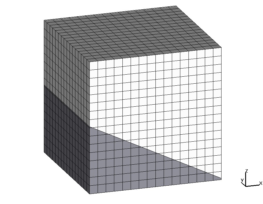
Figure 8: The matrix and fracture in the test with contaminant transport along the fracture.

The matrix–fracture configuration for this test is shown in Figure 8, $\Omega=(0,1)^{3}$, and $\Gamma=\{\mathbf{x}\in\Omega\,:\,z+\frac{1}{2}x=0.51\}$. The boundary $x=0$ is inflow, in the fracture the wind is constant $\mathbf{w}_{\Gamma}=(w_{1},0,w_{3})$, $|\mathbf{w}_{\Gamma}|=1$, and the contaminant source occupies the part of $\partial\Gamma$, ${\partial\Gamma}_{D}=\{(0,y,0.51)\,:\,y\in(\frac{1}{4},\frac{3}{4})\}$, $v_{D}=1$ on ${\partial\Gamma}_{D}$. We assume that the porous matrix is almost impermeable and so we set $\mathbf{w}_{i}=0$ in $\Omega_{i}$ (no flow in the rock) and $D_{i}=10^{-6}I$, $i=1,2$, ${\partial\Omega}={\partial\Omega}_{N}$. In the fracture we assume isotropic diffusion with $D_{\Gamma}=10^{-4}I$. Other parameters are the same as in the previous test, and $v=0$, $u=0$ at $t=0$. Therefore, we expect that the contaminant transport happens along the fracture with very small diffusion to the porous matrix. This is a bulk–surface variant of a standard test case of numerical solvers for convection–diffusion problems [50], and one is typically interested in the ability of a method to capture the right position and the shape of the sharp propagating front and avoid spurious oscillations. For a comparison purpose, one may consider the exact solution for the problems posed in a half-plane (or half-space) from [31, 32]. This solution $C(x,y,0)$ is given in (34), it solves $C_{t}-D\Delta C+{C}_{x}=0$ in $\widetilde{\Omega}=\{{(x,y)}\in\mathbb{R}^{2}\,:\,x>0\}$, with the boundary condition $C(0,y,t)=\left\{\begin{array}[]{c}c_{0},\textrm{ when }|y|<a,\\ 0,\textrm{ when }|y|>a,\end{array}\right.$and initial conditions: $C(x,y,0)=0$ in $\widetilde{\Omega}$.

$$C(x,y,t)=\frac{xc_{0}}{(16\pi D)^{\frac{1}{2}}}\int\limits_{0}^{t}\tau^{-\frac{3}{2}}\left\{\mathbf{erf}\left[\frac{a+y}{(4D\tau)^{\frac{1}{2}}}\right]+\mathbf{erf}\left[\frac{a-y}{(4D\tau)^{\frac{1}{2}}}\right]\right\}\cdot\mathbf{exp}\left[-\left(\frac{x-\tau}{(4D\tau)^{\frac{1}{2}}}\right)^{2}\right]d\tau.$$ (34)

where

$$\mathbf{erf}(x)=\frac{2}{\sqrt{\pi}}\int\limits_{0}^{x}e^{-t^{2}}dt,\quad\mathbf{erfc}(x)=1-\mathbf{erf}(x)=\frac{2}{\sqrt{\pi}}\int\limits_{x}^{\infty}e^{-t^{2}}dt.$$

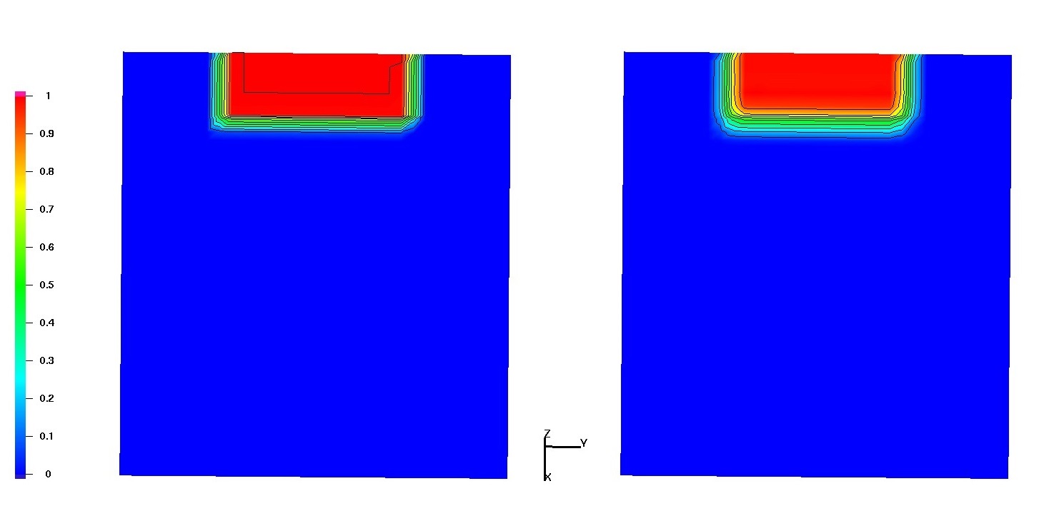
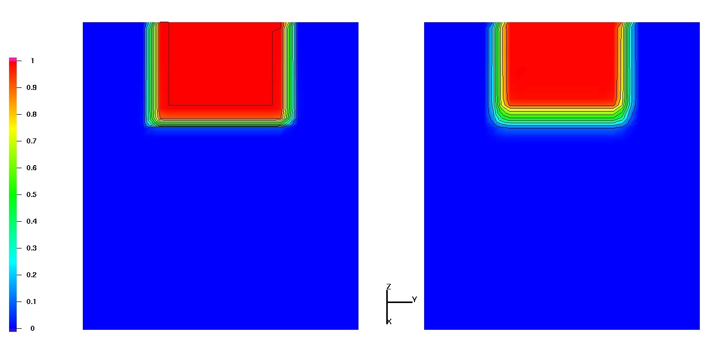
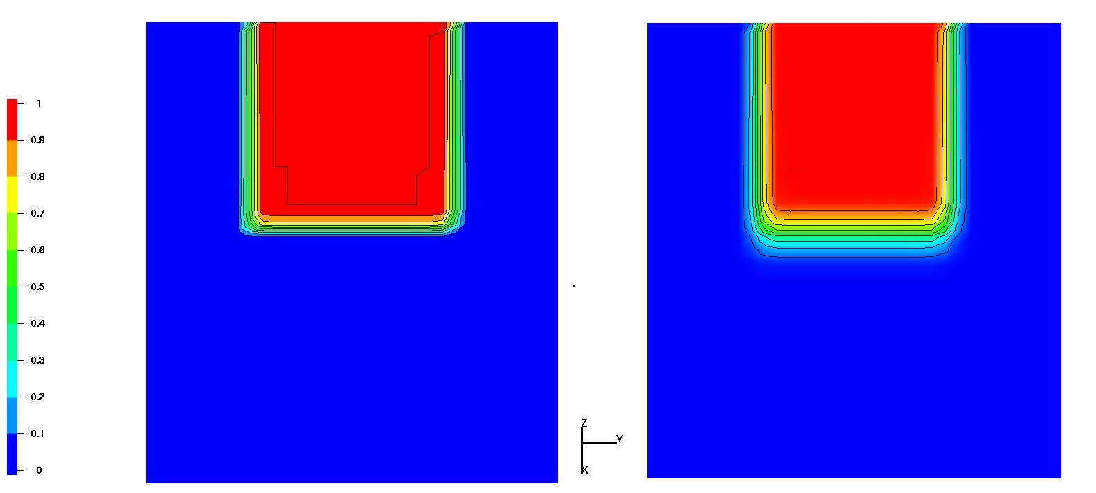
Figure 9: Reference 2D solution (left) and the fracture component of the computed solution (right) for the contaminant transport along the fracture test case. The solutions is shown for the times $t=0.17,\,0.34,\,0.5$.

We run our simulations with the uniform background mesh, $h=\frac{1}{32}$, $\Delta t=10^{-2}$. The fracture cuts through the background mesh as illustrated in Figure 8 (for better visualization, this figure shows the background mesh for $h=\frac{1}{16}$). The computed solution and the ‘reference’ solution is shown in Figure 9 at several time instances. We recall that the coupled problem was solved and the contaminant also diffuses into the bulk, but this bulk diffusion was minor. We observe that the computed solution well approximates the reference one; the computed front has the correct position and is not smeared too much. Moreover, we do not observe overshoots or undershoots in $v_{h}$.

4.4 An example with a spherical drop immersed in a bulk

We include one more test case but now with a different interface condition. This is the instantaneous absorbtion–desorption condition (9) with the Henry law to define $g_{i}$ and $f_{i}$. This condition is common in the literature to model dissolvable surfactant transport in two-phase flows. In this test from [24] we consider a prototypical configuration for such models consisting of a spherical drop embedded in a cubic domain. We take $\Gamma$ to be the unit sphere centered at the origin and $\Omega=[-1.2,1.2]^{3}$. By $\Omega_{1}$ we denote the interior of $\Gamma$, so $\Omega_{1}$ is the unit ball, $\Omega_{2}=\Omega\setminus\overline{\Omega}_{1}$. For the velocity field we take a rotating field in the $x$-$z$ plane: $\mathbf{w}=\frac{1}{10}(z,0,-x)$. This $\mathbf{w}$ satisfies $\mbox{\rm div}\mathbf{w}=0$ in $\Omega$ and $\mathbf{w}\cdot\mathbf{n}=0$ on $\Gamma$, i.e. the velocity field is everywhere tangential to the boundary and hence the steady interface is consistent with the kinematic condition: $\mathbf{w}\cdot\mathbf{n}$ is equal to the normal velocity of $\Gamma$ for immersible two-pase fluids, e.g. [25]. We set $\mathbf{w}_{i}=\mathbf{w}|_{\Omega_{i}}$ and $\mathbf{w}_{\Gamma}=\mathbf{w}|_{\Omega_{\Gamma}}$.

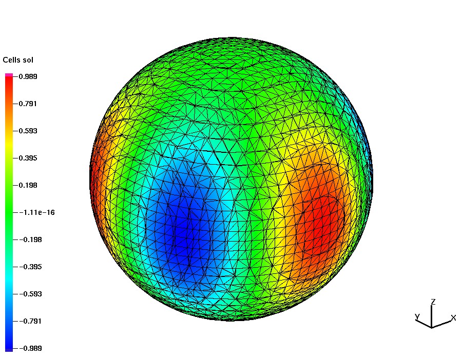
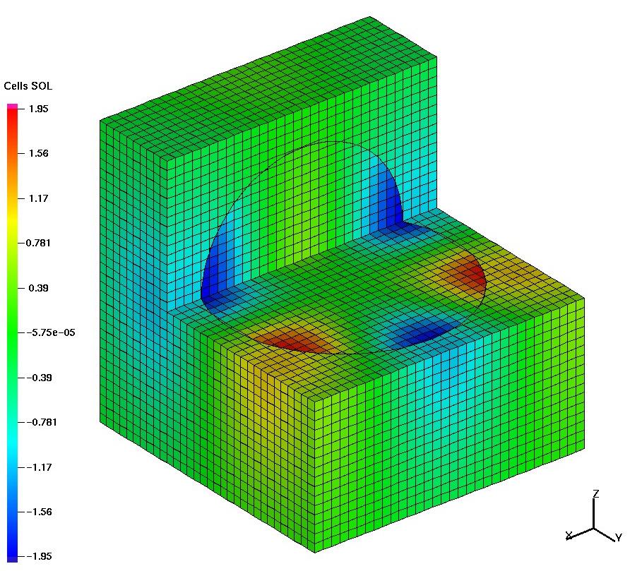
Figure 10: Left: Induced surface mesh and the surface component of computed solution. Right: Cut of the bulk mesh and the volume component of computed solution.

The material parameters are chosen as $D_{1}=0.5$, $D_{2}=1$, $D_{\Gamma}=1$ and $k_{1,a}=0.5$, $k_{2,a}=2$, $k_{1,d}=2$, $k_{2,d}=1$, $d=1$. The source terms $f_{i}\in L^{2}(\Omega)$, $i=1,2$, and $f_{\Gamma}\in L^{2}(\Gamma)$ and data on ${\partial\Omega}$ are taken such that the exact solution of the stationary equations (1)–(2) is given by

$$v(x,y,z)=3x^{2}y-y^{3},\quad u_{1}(x,y,z)=2u_{2}(x,y,z),\quad u_{2}(x,y,z)=e^{1-x^{2}-y^{2}-z^{2}}v(x,y,z).$$

Since we solve for a steady-state solution, so we set $\phi_{1}=\phi_{2}=\phi_{\Gamma}=0$. We prescribe Dirichlet boundary conditions on $\partial\Omega$, i.e. $\partial\Omega_{N}=\emptyset$, $\partial\Gamma_{N}=\emptyset$, and $\partial\Gamma_{D}=\emptyset$ in (7). Conditions (4)–(6) for this test case are not relevant, since the surface is globally smooth and has no boundary.

Table 5: Convergence of numerical solutions in the experiment with a spherical $\Gamma$ embedded in a cube.

	#d.o.f.	$L^{2}$-norm	rate	$H^{1}$-norm	rate	$L^{\infty}$-norm	rate
$\Omega$	736	3.223e-02		9.706e-01		1.072e-01
	4920	6.687e-03	2.27	1.555e-01	2.64	3.799e-02	1.50
	36088	2.005e-03	1.74	5.363e-02	1.55	9.180e-01	-4.59
	275544	5.055e-04	1.99	1.825e-02	1.56	2.777e-03	8.37
$\Gamma$	460	1.670e-02		2.065e-01		3.863e-02
	1660	4.037e-03	2.05	9.647e-02	1.10	1.060e-02	1.87
	6628	9.211e-04	2.13	4.745e-02	1.02	3.881e-03	1.45
	26740	2.457e-04	1.91	2.396e-02	0.99	8.875e-04	2.13

In this set of experiments we take the sequence of uniform cubic meshes in $\Omega$, starting with $h=0.3$. The surface $\Gamma_{h}$ is reconstructed as described in section 3.2 for $\phi(\mathbf{x})=1-|\mathbf{x}|^{2}$. The computed solution as well as volume and induced surface meshes are illustrated in Figure 10. The computed errors for the bulk and surface concentrations are shown in Table 5. For this example, the method demonstrates optimal convergence: $O(h)$ in the $H^{1}$ and $O(h^{2})$ in the $L^{2}$ and surface norms. This is consistent with what is known about the convergence of the TraceFEM for linear bulk elements, see e.g. analysis and convergence rates for the same experiment in [24], where the TraceFEM has been used to discretized equations both on the surface and in the bulk. For the volume component of the solution, the convergence is close to the second order in the $L^{2}$ norm and $1.5$ order in the $H^{1}$ norm. It is also consistent with the results in [35], where super-convergence of the method in the $H^{1}$ norm was observed. Convergence in the $L^{\infty}$-norm is somewhat less regular. We note that the $L^{\infty}$ convergence of the TraceFEM and of the non-linear FV method that we used has not been studied before.

The aim of the next (final) test is to illustrate the performance of the method for the case of locally refined grids. The setup is similar to the test with the sphere above, but the coefficients and the known solution are taken different to represent the situation of a convection dominated problem with an internal layer. More precisely, for the velocity field we take $\mathbf{w}=(-y\sqrt{1-z^{2}},x\sqrt{1-z^{2}},0)$, and set $\mathbf{w}_{i}=\mathbf{w}|_{\Omega_{i}}$ and $\mathbf{w}_{\Gamma}=\mathbf{w}|_{\Omega_{\Gamma}}$.

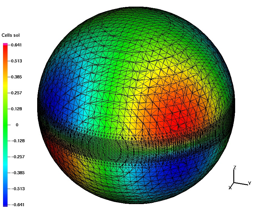
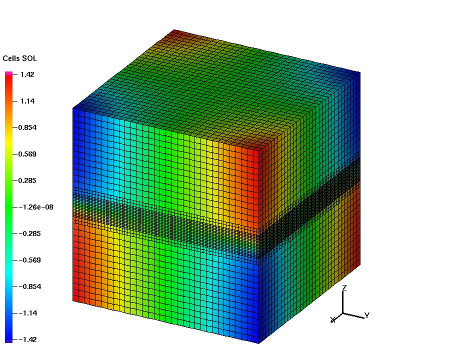
Figure 11: Left: Induced surface mesh and the surface component of computed solution. Right: The bulk mesh and the volume component of computed solution.

The material parameters are chosen as $D_{1}=D_{2}=D_{\Gamma}=\varepsilon$ and $k_{1,a}=0.5$, $k_{2,a}=2$, $k_{1,d}=2$, $k_{2,d}=1$, $d=1$. The source terms $f_{i}\in L^{2}(\Omega)$, $i=1,2$, and $f_{\Gamma}\in L^{2}(\Gamma)$ and data on ${\partial\Omega}$ are taken such that the exact solution of the stationary equations (1)–(2) is given by

$$v(x,y,z)={xz}\mathrm{arctan}\left(\frac{2z}{\sqrt{\varepsilon}}\right),\quad u_{1}(x,y,z)=2u_{2}(x,y,z),\quad u_{2}(x,y,z)=e^{1-x^{2}-y^{2}-z^{2}}v(x,y,z).$$

We take $\varepsilon=1$ (very smooth solution) and $\varepsilon=0.01$ (solution has an internal layer along the midplane $z=0$).

Table 6: Convergence of numerical solutions in the experiment with a spherical $\Gamma$ and locally refined mesh.

	$\varepsilon=1$						$\varepsilon=1e-2$
#d.o.f.	$L^{2}$-norm	rate	$H^{1}$-norm	rate	$L^{\infty}$-norm	rate	$L^{2}$-norm	rate	$H^{1}$-norm	rate	$L^{\infty}$-norm	rate
$\Omega$
5840	3.993e-03		8.322e-02		1.706e-02		5.666e-02		3.987e-01		1.945e-01
43552	6.706e-04	2.57	2.828e-02	1.56	4.926e-03	1.79	2.609e-02	1.12	2.440e-01	0.71	8.403e-02	1.21
318696	2.200e-04	1.61	1.038e-02	1.45	2.158e-02	-2.13	1.353e-02	0.95	1.708e-01	0.52	5.003e-02	0.75
$\Gamma$
1500	1.916e-03		3.609e-02		6.850e-03		8.353e-03		4.026e-01		4.538e-02
6740	5.106e-04	1.91	1.710e-02	1.08	1.919e-03	1.84	1.854e-03	2.17	1.619e-01	1.31	1.335e-02	1.76
25988	1.400e-04	1.87	8.924e-03	0.94	5.624e-04	1.77	3.848e-04	2.26	6.532e-02	1.31	3.694e-03	1.85

We build a sequence of locally refined meshes as illustrated in Figure 11. For $\varepsilon=0.01$ the meshes are fitted to the layer and intend to capture the sharp variation of the solution. We computed numerical solutions on a sequence of 3 meshes, the second mesh is illustrated in  Figure 11. Each mesh has two levels of refinement in the region $|z|<\frac{1}{8}$. The convergence of the method is reported in Table 6. The optimal order of convergence is attended for the surface component of the solution, but the FV method in the bulk domain shows lower order convergence for the convection dominated case. We conclude that more studies are required to improve the performance of the FV method on such type of meshes.

5 Conclusions

The paper proposed a hybrid finite volume – finite element method for the coupled bulk–surface systems of PDEs. The distinct feature of the method is that the same background mesh is used to solve equations in the bulk and on the surfaces, and that there is no need to fit this mesh to the embedded surfaces. This makes the approach particularly attractive to treat problems with complicated embedded structures of lower dimension like those occurring in the simulations of flow and transport in fractured porous media. We consider the particular monotone non-linear FV method with compact stencil, but we believe that the approach can be carried over and used with other FV methods on polyhedral meshes (e.g. some of those reviewed in [16]) with possibly better performance in terms of convergence rates. In this paper we treated only diffusion and transport of a contaminant assuming that Darcy velocity is given. Extending the method to computing flows in fractured porous media is in our future plans together with the design of better algebraic solvers, doing research on adaptivity, and adding to the method a fracture prorogation model.

Acknowledgments

The work of the first author (the numerical implementation and the numerical experiments) has been supported by the Russian Scientific Foundation Grant 17-71-10173, the work of the second author has been supported by the NSF grant 1717516, the work of the third author has been supported by the RFBR grant 17-01-00886.

References

- [1] C. Alboin, J. Jaffré, J. E. Roberts, and C. Serres. Modeling fractures as interfaces for flow and transport. In Fluid Flow and Transport in Porous Media, Mathematical and Numerical Treatment, volume 295, page 13. American Mathematical Soc., 2002.
- [2] P. Angot, F. Boyer, and F. Hubert. Asymptotic and numerical modelling of flows in fractured porous media. ESAIM: Mathematical Modelling and Numerical Analysis, 43(2):239–275, 2009.
- [3] W. Bangerth, D. Davydov, T. Heister, L. Heltai, G. Kanschat, M. Kronbichler, M. Maier, B. Turcksin, and D. Wells. The deal.ii library, version 8.4. Journal of Numerical Mathematics, 24:135–141, 2016.
- [4] J. W. Barrett, H. Garcke, and R. Nürnberg. On the stable numerical approximation of two-phase flow with insoluble surfactant. ESAIM: Mathematical Modelling and Numerical Analysis, 49(2):421–458, 2015.
- [5] J. W. Barrett, H. Garcke, and R. Nürnberg. Stable finite element approximations of two-phase flow with soluble surfactant. Journal of Computational Physics, 297:530–564, 2015.
- [6] M. Bertalmio, L. Cheng, S. Osher, and G. Sapiro. Variational problems and partial differential equations on implicit surfaces: The framework and examples in image processing and pattern formation. J. Comput. Phys., 174:759–780, 2001.
- [7] A. Bonito, R. Nochetto, and M. Pauletti. Dynamics of biomembranes: effect of the bulk fluid. Mathematical Modelling of natural phenomena, 6(05):25–43, 2011.
- [8] E. Burman, S. Claus, P. Hansbo, M. G. Larson, and A. Massing. Cutfem: Discretizing geometry and partial differential equations. International Journal for Numerical Methods in Engineering, 104(7):472–501, 2015.
- [9] M. Cenanovic, P. Hansbo, and M. G. Larson. Cut finite element modeling of linear membranes. Computer Methods in Applied Mechanics and Engineering, 310:98–111, 2016.
- [10] K.-Y. Chen and M.-C. Lai. A conservative scheme for solving coupled surface-bulk convection–diffusion equations with an application to interfacial flows with soluble surfactant. Journal of Computational Physics, 257:1–18, 2014.
- [11] A. Chernyshenko and Y. Vassilevski. A finite volume scheme with the discrete maximum principle for diffusion equations on polyhedral meshes. In J. Fuhrmann, M. Ohlberger, and C. Rohde, editors, Finite Volumes for Complex Applications VII-Methods and Theoretical Aspects, Springer Proceedings in Mathematics and Statistics, volume 77, pages 197–205. Springer International Publishing, Switzerland, 2014.
- [12] A. Y. Chernyshenko and M. A. Olshanskii. An adaptive octree finite element method for pdes posed on surfaces. Computer Methods in Applied Mechanics and Engineering, 291:146–172, 2015.
- [13] A. Danilov and Y. Vassilevski. A monotone nonlinear finite volume method for diffusion equations on conformal polyhedral meshes. Russian J. Numer. Anal. Math. Modelling, 24(3):207–227, 2009.
- [14] F. Dassi, S. Perotto, L. Formaggia, and P. Ruffo. Efficient geometric reconstruction of complex geological structures. Mathematics and Computers in Simulation, 106:163–184, 2014.
- [15] K. Deckelnick, C. M. Elliott, and T. Ranner. Unfitted finite element methods using bulk meshes for surface partial differential equations. arXiv preprint arXiv:1312.2905, 2013.
- [16] J. Droniou. Finite volume schemes for diffusion equations: introduction to and review of modern methods. Math. Models Methods Appl. Sci., 24(8):1575–1619, 2014.
- [17] J. Droniou and C. Le Potier. Construction and convergence study of schemes preserving the elliptic local maximum principle. SIAM J. Numer. Anal., 49(2):459–490, 2011.
- [18] C. M. Elliott and T. Ranner. Finite element analysis for coupled bulk-surface partial differential equation. IMA J Numer Anal, 33:377–402, 2013.
- [19] B. Flemisch, A. Fumagalli, and A. Scotti. A review of the xfem-based approximation of flow in fractured porous media. In Advances in Discretization Methods, pages 47–76. Springer, 2016.
- [20] N. Frih, V. Martin, J. E. Roberts, and A. Saâda. Modeling fractures as interfaces with nonmatching grids. Computational Geosciences, pages 1–18, 2012.
- [21] J. Fuhrmann, M. Ohlberger, and C. Rohde, editors. Finite Volumes for Complex Applications VII, Springer Proceedings in Mathematics and Statistics, volume 77. Springer International Publishing, Switzerland, 2014.
- [22] A. Fumagalli and A. Scotti. A reduced model for flow and transport in fractured porous media with non-matching grids. In Numerical Mathematics and Advanced Applications 2011, pages 499–507. Springer, 2013.
- [23] Z. Gao and J. Wu. A small stencil and extremum preserving scheme for anisotropic diffusion problems on arbitrary 2d and 3d meshes. J.Comp.Phys., 250:308–331, 2013.
- [24] S. Gross, M. A. Olshanskii, and A. Reusken. A trace finite element method for a class of coupled bulk-interface transport problems. ESAIM: Mathematical Modelling and Numerical Analysis, 49(5):1303–1330, 2015.
- [25] S. Gross and A. Reusken. Numerical methods for two-phase incompressible flows, volume 40. Springer-Verlag, 2011.
- [26] P. Hansbo, M. G. Larson, and S. Zahedi. A cut finite element method for coupled bulk-surface problems on time-dependent domains. Computer Methods in Applied Mechanics and Engineering, 307:96–116, 2016.
- [27] C.-C. Ho, F.-C. Wu, B.-Y. Chen, Y.-Y. Chuang, and M. Ouhyoung. Cubical marching squares: Adaptive feature preserving surface extraction from volume data. EUROGRAPHICS 2005 / M. Alexa and J. Marks (Guest Editors), 24(3), 2005.
- [28] I. Kapyrin, K. Nikitin, K. Terekhov, and Y. Vassilevski. Nonlinear monotone FV schemes for radionuclide geomigration and multiphase flow models. In J. Fuhrmann, M. Ohlberger, and C. Rohde, editors, Finite Volumes for Complex Applications VII-Elliptic, Parabolic and Hyperbolic Problems, Springer Proceedings in Mathematics and Statistics, volume 77, pages 655–663. Springer International Publishing, Switzerland, 2014.
- [29] Y.-I. Kwon and J. Derby. Modeling the coupled effects of interfacial and bulk phenomena during solution crystal growth. J. Cryst. Growth, 230(1):328–335, 2001.
- [30] C. Le Potier. Finite volume scheme satisfying maximum and minimum principles for anisotropic diffusion operators. In R. Eymard and J.-M. Herard, editors, Finite Volumes for Complex Applications V, pages 103–118, 2008.
- [31] F. J. Leij and J. Dane. Analytical solutions of the one-dimensional advection equation and two-or three-dimensional dispersion equation. Water resources research, 26(7):1475–1482, 1990.
- [32] F. J. Leij, T. H. Skaggs, and M. T. Van Genuchten. Analytical solutions for solute transport in three-dimensional semi-infinite porous media. Water resources research, 27(10):2719–2733, 1991.
- [33] H. Levine and W.-J. Rappel. Membrane-bound turing patterns. Physical Review E, 72(6):061912, 2005.
- [34] K. Lipnikov, D. Svyatskiy, and Y. Vassilevski. A monotone finite volume method for advection-diffusion equations on unstructured polygonal meshes. J. Comp. Phys., 229:4017–4032, 2009.
- [35] K. Lipnikov, D. Svyatskiy, and Y. Vassilevski. Minimal stencil finite volume scheme with the discrete maximum principle. Russian J. Numer. Anal. Math. Modelling, 27(4):369–385, 2012.
- [36] A. Madzvamuse and A. H. Chung. The bulk-surface finite element method for reaction–diffusion systems on stationary volumes. Finite Elements in Analysis and Design, 108:9–21, 2016.
- [37] A. Madzvamuse, A. H. Chung, and C. Venkataraman. Stability analysis and simulations of coupled bulk-surface reaction–diffusion systems. In Proc. R. Soc. A, volume 471, page 20140546. The Royal Society, 2015.
- [38] V. Martin, J. Jaffré, and J. E. Roberts. Modeling fractures and barriers as interfaces for flow in porous media. SIAM Journal on Scientific Computing, 26(5):1667–1691, 2005.
- [39] J. Maryška, O. Severỳn, and M. Vohralík. Numerical simulation of fracture flow with a mixed-hybrid fem stochastic discrete fracture network model. Computational Geosciences, 8(3):217–234, 2005.
- [40] K. Nikitin and Y. Vassilevski. A monotone nonlinear finite volume method for advection-diffusion equations on unstructured polyhedral meshes in 3d. Russian J. Numer. Anal. Math. Modelling, 25(4):335–358, 2010.
- [41] M. Olshanskii, A. Reusken, and J. Grande. A finite element method for elliptic equations on surfaces. SIAM J. Numer. Anal., 47:3339–3358, 2009.
- [42] M. Olshanskii, A. Reusken, and X.Xu. A stabilized finite element method for advection-diffusion equations on surfaces. IMA J Numer. Anal., 34:732–758, 2014.
- [43] M. Olshanskii and D. Safin. A narrow-band unfitted finite element method for elliptic pdes posed on surfaces. Mathematics of Computation, 85(300):1549–1570, 2016.
- [44] M. A. Olshanskii and A. Reusken. Trace finite element methods for pdes on surfaces. arXiv preprint arXiv:1612.00054, 2016.
- [45] S. Popinet. Gerris: a tree-based adaptive solver for the incompressible Euler equations in complex geometries. J. Comput. Phys., 190:572–600, 2003.
- [46] A. Rätz and M. Röger. Turing instabilities in a mathematical model for signaling networks. J. Math. Biol., 65(6):1215–1244, 2012.
- [47] F. Ravera, M. Ferrari, and L. Liggieri. Adsorption and partitioning of surfactants in liquid–liquid systems. Advances in Colloid and Interface Science, 88(1):129–177, 2000.
- [48] A. Reusken. Analysis of trace finite element methods for surface partial differential equations. IMA Journal of Numerical Analysis, 35(4):1568–1590, 2015.
- [49] Z. Sheng and G. Yuan. The finite volume scheme preserving extremum principle for diffusion equations on polygonal meshes. J. Comput. Phys., 230(7):2588–2604, 2011.
- [50] N.-Z. Sun and A. Sun. Mathematical modeling of groundwater pollution. Springer Science & Business Media, 2013.
- [51] K. E. Teigen, X. Li, J. Lowengrub, F. Wang, and A. Voigt. A diffuse-interface approach for modeling transport, diffusion and adsorption/desorption of material quantities on a deformable interface. Communications in mathematical sciences, 4(7):1009, 2009.
- [52] R. Therrien and E. Sudicky. Three-dimensional analysis of variably-saturated flow and solute transport in discretely-fractured porous media. Journal of Contaminant Hydrology, 23(1):1–44, 1996.