Legendre Analysis of Differential
Distributions
in Hadronic Reactions
Yakov I. Azimov
Petersburg Nuclear Physics Institute, NRC
Kurchatov Institute, Gatchina, 188300, Russia
Igor I. Strakovsky
igor@gwu.eduThe George Washington University, Washington,
DC 20052, USA
William J. Briscoe
The George Washington University, Washington,
DC 20052, USA
Ron L. Workman
The George Washington University, Washington,
DC 20052, USA
Abstract
Abstract
Modern experimental facilities, such as CBELSA, ELPH, JLab, MAMI and SPring-8
have provided a tremendous volume of data, often with wide energy and angular
coverage, and with increasing precision. For reactions with two hadrons in the final
state, these data are often presented as multiple sets of panels, with
angular distributions at numerous specific energies. Such presentations have
limited visual appeal, and their physical content is typically extracted through some
model-dependent treatment. Instead, we explore the use of a
Legendre series expansion with a relatively small number of essential coefficients.
This approach has been applied in several recent experimental investigations.
We present some general properties
of the Legendre coefficients in the helicity framework and consider what
physical information can be extracted without any model-dependent assumptions.
pacs:
12.38.Aw, 13.60.Rj, 14.20.-c, 25.20.Lj
I Introduction
Modern detectors, combined with the present generation of
accelerator facilities, are capable of
providing large reaction-specific sets of experimental data.
These sets have often been combined in partial-wave analyses
with the hope of extracting elements of the fundamental reaction
process (such as resonance parameters and coupling constants).
The analyses generally have some model-dependence and are limited
by the quality of the available data.
Here we address the problem of displaying these large data sets,
evaluating their physical content, and determining their sensitivity
to partial-wave content in a model-independent manner.
Even in relatively
simple cases of reactions, data are usually presented
as multi-panel pictures with a great number of angular distributions
for different energies (and/or energy distributions for different angles).
Such an approach can be used, of course, to compare with various models,
but is not practical for any direct extraction of physical information.
In several recent works, we and others have suggested and applied another approach,
involving the expansion of differential cross sections, for both
unpolarized CBC ; A2 and polarized CLAS photoproduction
of single pseudoscalar mesons, in terms of Legendre coefficients. For
a limited energy interval, it appears sufficient to use a finite
number of the expansion terms, which may be plotted as a function of energy,
thus providing a more clear and visually suggestive
presentation, which may be further analyzed through models or partial-wave
analyses.
Preliminary results of this study were reported at the Hadron
Structure and QCD: from Low to High Energies Workshop YaA16 .
In the present paper, we further describe and study this
approach more systematically. Then we discuss its utility for the
extraction of model-independent information.
II Expansion of Amplitudes and Cross Sections
Let us consider reaction
(1)
where particles have spins . It can be described
by helicity amplitudes jw
,
where and are the
corresponding -channel helicities, is the center-of-mass (c.m.)
energy, and . The angles and are, respectively,
the polar and azimuthal c.m. angles. These amplitudes may be decomposed
in terms of the Wigner harmonics
(2)
(3)
with partial-wave amplitudes
(4)
being elements of the -matrix, related to the -matrix,
, being the initial relative c.m. momentum, and
(5)
The scattering/production angle is taken to be the angle
between the c.m. momenta of particles and (or and ).
All the values of are simultaneously either integer
or half-integer and the above -summation runs over all physical values of
.
The differential cross section, with all
initial and final helicities fixed, is jw
(6)
Note that is independent of the azimuthal angle
, since every particular helicity amplitude depends on
only through a phase factor.
The totally unpolarized differential cross section can be written as
(7)
(8)
where implies summation over all initial and final
helicities. We separate out the normalization factor , which has a simple
structure, with a known dependence on the energy and on the
spins (due to summing and averaging over polarization states), but is
quite independent of any dynamics, helicities, angles, and angular momenta
(it is not essential for the following discussion). The angular
dependence of each summand in Eq.(8) is completely described
by two -harmonics with the same and . Their product
can be decomposed into a Clebsch-Gordan series over the Legendre
polynomials. As a result, we obtain
(9)
with integer . According to the composition rules for angular momenta,
every contains bilinear contributions of partial-wave
amplitudes (see Eq.(8)) with angular momenta and
satisfying the familiar relations
(10)
This means that a particular Legendre coefficient
generally contains an infinite number of contributions from partial-wave amplitudes
with various -values. But it evidently can not contain interference of
amplitudes with too different and (i.e., with ).
Quadratic terms, having , may appear only at sufficiently large
. Of course, the coefficient coincides with half
the total cross section of reaction (1) at the energy .
Recall that if one fits
.
The Legendre coefficients have another, less evident, property. To derive it, we
combine Eqs.(A1), (A2), and (41) of Ref. jw and obtain
(11)
(12)
Here ,
and are the internal parities of the particles and ;
is the space reflection operator. The amplitudes have the
same structure as (see Eq.(3)), but the partial-wave
amplitudes are taken with the space-reflected initial states. The first factor
in the right-hand side of Eqs.(11) and (12) is independent of
and, when squared, is always unity, since is always an integer.
Of course, these relations could be rewritten in a different form, with space
reflection affecting the final (instead of initial) states.
Now we can write the differential cross section in two forms:
(13)
where has the same structure as ,
but helicity summation uses space-reflected initial (or final) states. Since
, we derive
(14)
If the states used in the summation are separated by their parities, then this
equality means that -coefficients with odd -values
may contain only contributions which are bilinear in states of opposite parities.
For even , on the other hand, bilinear contributions also appear in the
, but only with both states of the same parity, positive or
negative. Quadratic contributions of any state can appear only at even .
This means, in particular, that proper Breit-Wigner (BW) contributions of a
resonance of an integer spin appear in the even- Legendre
coefficients with . But if the spin is half-integer,
these BW contributions do not appear at ; they appear only at
even with .
The above expressions clearly demonstrate the well-known statement that the
unpolarized cross section by itself does not allow a determination of the parity of a
particular partial wave, since simultaneous reversal of parities for
all partial waves does not influence the cross section. However, if
there is a resonance with known quantum numbers, including its parity, then
such complete parity reversal becomes impossible, and even unpolarized cross
section is able to provide some information on partial-wave parities. Below
we will discuss this point in more detail.
Described above is the Legendre decomposition for the unpolarized
differential cross sections. However, such an approach may be applied
also to processes with polarized particles and/or to polarization
observables (more exactly, to polarization observables multiplied by the
unpolarized differential cross section). Such quantities may kinematically
vanish at (they may even have square root singularities there).
Decomposition in Legendre polynomials then becomes inadequate, and one
should instead use Wigner harmonics (or, in particular, associated
Legendre polynomials) with integer . For example, the beam asymmetry
studied by the CLAS Collaboration CLAS contains the kinematical
factor which automatically arises in any converging series over
the associated Legendre polynomials ). In such cases the
decomposition retains connection (10) between and ;
relation (11) again allows one to separate interferences of states with
the same or with opposite parities.
Let us briefly discuss one more point. The series (3) and
(9) generally sum an infinite number of terms. In practical cases,
the series will be truncated. This may be justified on the basis of physical
reasons (e.g., presence of pronounced resonances in the data,
with known definite spins and parities) or phenomenological ones
(e.g., higher Legendre coefficient may be safely discarded if their
fitting errors exceed fitted values). In both cases, we obtain a
limited number of parameters to describe experimental data and to
investigate their physical content.
III Photoproduction of a Spinless Meson
To illustrate the above approach, we consider in more detail the
particular case of a pseudoscalar-meson photoproduction off the proton,
for instance,
(15)
The initial state has four possible helicity combinations (), while the final state has two helicity
combinations (). Thus, there are eight
different transitions between various initial and final helicities and,
generally, eight different helicity amplitudes.
It is interesting to emphasize that the value of unambiguously
determines all initial helicities: if , then
; if , then
(of course, this is due to
absence of ). Hence, the independent amplitudes may
be denoted as , where the sign in the index is the
sign of , opposite to the sign of helicity of the final nucleon.
Expression (8) for the unpolarized cross section may be
rewritten as
(16)
with -summation over four values . The initial
state with a particular value of can be realized by using the
circularly polarized photon (with a definite helicity) together with the
longitudinally polarized target nucleon. Therefore, also measurable is the
cross section for any fixed :
(17)
The additional factor 4, as compared to Eq.(16), arises since
deals with a single initial state, while the
unpolarized expression (16) implies averaging over four initial
states with different helicities.
Note that amplitudes with all helicities reversed are related by parity
conservation jw , so that only four of the eight amplitudes are
independent. Eq.(44) of Ref. jw , applied to the photoproduction reaction,
gives
(18)
Therefore, we can use only amplitudes with positive values of . For negative values of we have
As a result,
due to parity conservation. Moreover,
(19)
Difference of the helicity cross sections is related to the double polarization
observable :
(20)
Following Walker Walker , if we let to label the
four independent helicity amplitudes,
the translation to amplitudes of the form
is given in Table 1.
Table 1: Walker notation Walker for
helicity amplitudes .
H1
H2
H4
-H3
H3
H4
-H2
H1
Partial-wave decomposition of the amplitudes contains
the partial-wave helicity amplitudes which may be analogously denoted as
, with the same meaning of indices; note that
for , while for .
Further, the helicity partial-wave amplitudes can be combined so to obtain two
sets of definite-parity partial-wave amplitudes .
According to Eq.(41) of Ref. jw , we obtain
(21)
where or 3/2 , the upper sign corresponds to the final
(and initial as well) state parity equal to , and
are intrinsic parities of the pion and nucleon. The inverted expressions are
(22)
Of course, . Recall also that
the lower sign or corresponds to the final state value ,
while the upper sign corresponds to parity of the final (and initial) state.
It is easy to check that
(23)
(24)
In particular,
(recall that here all the -values are half-integer, so is always
an integer).
The translation from these partial-wave amplitudes to the helicity elements,
and ,
as well as the multipole amplitudes, and ,
is given in Ref. Walker . For
example, we have
(25)
(26)
where the subscript notation for helicity elements and
multipoles CGLN denotes a state with orbital
angular momentum and total angular momentum .
The above analysis is equally applicable for the process of the -meson
photoproduction
(27)
(or for photoproduction). The energy region of
production, investigated experimentally in Ref. CBC , is assumed to contain
resonances with spins up to 5/2 PDG . One can expect, therefore, that
the decompositions should essentially run up to in Eq.(3)
and up to in Eq.(9). Such an
expectation agrees with the fit to
data CBC : extracted Legendre coefficients with appear to be
consistent with zero, within their uncertainties. The Wigner harmonics
necessary for the amplitude decompositions are given explicitly in
Appendix 1C. (Note that for the production, at
similar energies A2 ; CLAS , one needs more lengthy decompositions up
to , because of the lower associated threshold.)
Now we can illustrate our approach in more detail for the cross sections of
the reaction (27). We use Eq.(8) (truncated up to
) and decompositions of Appendix 1D to derive
expressions for the Legendre coefficients .
They are shown in Appendix 2A. Note that can be
rewritten in the form
(28)
the left-hand side factor 1/2 accounts for the fact that the right-hand side
expression contains contributions of only one sign of the total helicities,
and , while should contain also contributions
with the negative sign of helicities (recall that positive and negative sign
contributions are equal to each other, due to parity conservation). This
relation is true even without -truncating and clearly shows that
is indeed proportional to the total (i.e.,
integrated differential) cross section, as it should be.
Explicit expressions of Appendix 2A confirm the properties of the Legendre
coefficients formulated above. Every coefficient has two parts, corresponding
to and . Of course, states with contribute
only to . Coefficients with even consist of
proper contributions of various partial-wave states and interference
contributions of states with different , but with the same parities, both
positive and negative. On the other hand, the odd- coefficients contain
only interferences between states of the same or different values of , but
always with opposite parities, exactly as stated in the preceding Section.
As the value of increases, so does the number of contributions to
. The simple structure of and
in Appendix 2 is the result of our assuming the absence of
states with . In particular, it is because of this assumption that
states with are not seen in the displayed expressions for
and .
This approach can be easily applied to other polarization
observables. For example,
the double polarization observable may also
be expanded in Legendre polynomials , similar to Eq.(9),
but with different Legendre coefficients . Comparison of
expressions (19) and (20) shows that
and differ only in the sign of all contributions with
.
The beam-polarizaton quantity, , is also treated within the helicity
formalism in Ref. Walker ,
(29)
Both terms in the square brackets contain the kinematical edge factor
, and we expand them over the associated Legendre functions
with , which all have the same edge factor:
(30)
Application of property (12) to the right-hand side of expression
(29) shows that the coefficients also contain
parity correlations, just in the same way as the coefficients
for the unpolarized cross section.
Expansions for products of -harmonics, up to , arising in
Eq.(29) are given in Appendix 1E. They allow to obtain
with truncated at . The results are
shown in Appendix 2B. All contributions to the Legendre coefficients
come from interferences of amplitudes with initial
total helicities 1/2 and 3/2. State parities are correlated exactly as
for : the same parities in the even- coefficients
and opposite parities in the odd- ones. There is, however, an
interesting difference, not quite evident in expression (29).
Inversion of parities for all states does not change
and, therefore, the cross sections (differential and total). On the other
hand, such a transformation reverses the signs of all and,
therefore, of and as well.
IV Application to Data
The expansion method requires data of both high precision and broad
angular coverage to determine the higher-order coefficients.
A prime example is provided by
the A2 Collaboration at MAMI which recently reported
7978 data for the reaction
and for for incident photon energies from 218 to 1573 MeV
(or for c.m energies W = 1136 – 1957 MeV) A2 . These data are
obtained with a fine binning in (4 MeV for all energies
below E = 1120 MeV) and 30 angular bins, giving a good coverage of
the production angle. The data obtained above E = 1443 MeV
(W = 1894 MeV), however, have a limited angular coverage and for this
reason were excluded from the present Legendre fit.
A good description of the differential cross sections was obtained, for each included energy bin
and the full angular range, in a fit with Legendre
polynomials up to order ten (Eq.(9)) - the
coefficients depending on energy.
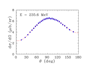
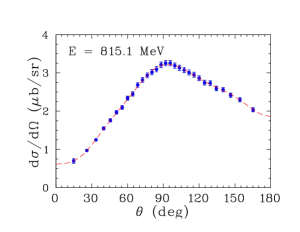
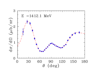
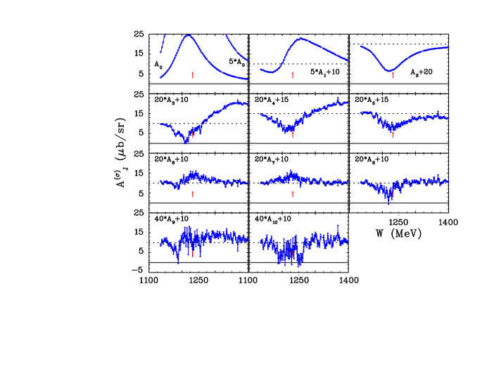
Figure 1: (Color online)
Top panel: Samples of the
differential cross sections, , from
A2 Collaboration
at MAMI measurements (blue filled circles) A2
with the best fit results using Legendre polynomials
(red dashed lines). The
error bars on all data points represent statistical
uncertaities only. Values of in each plot indicate
the lab photon energies.
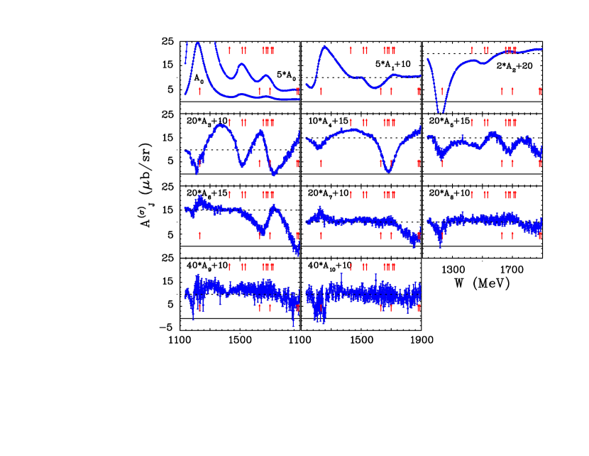
Bottom panel: Coefficients of Legendre
polynomials (blue filled circles). The error bars of
all values represent A uncertainties
from the fits in which only the statistical uncertainties
were used. Solid lines are plotted to help guide
the eye. Red vertical arrows indicate masses of the
four-star resonances (BW masses) known in this energy
range PDG . The upper row of arrows
corresponds to N∗ states with isospin and the
lower row corresponds to with .
The typical experimental statistics and the Legendre-polynomial
fits are illustrated in Fig. 1(top panel) for
different energies. The results of the Legendre-polynomial fits
for each coefficient are depicted in
Fig. 1(bottom panel), showing their energy
dependence in unprecedented detail.
As expected from the form of Eq.(28), resonance contributions
from the first, second and third resonance regions combine to
produce clear peaks in the coefficient .
These regions are somewhat less pronounced in , which
also contains interference terms between states of the same parity.
The result for itself shows
good agreement with the total cross section,
obtained by an integration of the differential cross sections,
confirming the quality of this dataset.
Other interesting features in Fig. 1, and the expanded
plot of Fig. 2, are the sharp structures seen for each
coefficient in the region of .
This resonance can contribute directly (without interference) only to
and . Since there exists no other
nearby resonance, such structures can appear only due to the
interference of with other non-resonant
partial-waves. Coefficient should reveal the
interference of with the three states having
, , and . Higher coefficients
could reveal interference with the four states
having , and , with parity
positive for even and negative for odd . Thus, via such
interference effects, the contributions from very high partial-wave
amplitudes could be studied, a possibility not available in any
other standard approach. This feature is similar to enhancing the
manifestation of rare decay modes of resonances via the interference
with other strong resonances YaA .
It should be noted that the recurring sharp structures associated with
the energy region do not appear in multipole analyses
of these data. The angle-independent systematic error was used to determine
renormalization factors for each angular distribution. These factors were
determined to be very near unity (within 1%) and, if applied to the
data, had no effect on the higher Legendre coefficients. If instead,
the statistical and systematic errors are added in quadrature Beck ,
structures in the highest coefficients are masked by greatly expanded errors.
This result emphasizes the importance of systematic error analysis, the
effect of which may also be magnified by a dominant resonance.
Figure 2: (Color online) Zoom for A2
data below W = 1400 MeV to cover the -isobar
region A2 as shown on
Fig. 1(bottom panel).
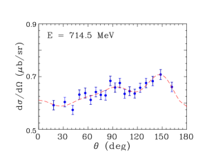
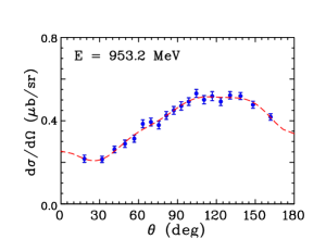
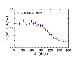
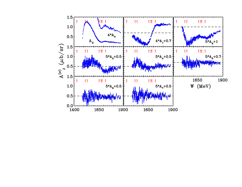
Figure 3: (Color online)
Top panel: Samples of the
differential cross sections, , from
A2 Collaboration
at MAMI measurements CBC with the
best fit results using Legendre polynomials. The
notation as given
in Fig. 1.
Bottom panel: Coefficients for Legendre
polynomials. The notation is given in
Fig. 1.
The A2 collaboration at MAMI has also measured
2400 s for the reaction and
for for incident photon energies from 710 and up to 1395 MeV
(or for c.m energies W = 1488 – 1870 MeV] CBC . The large
number of events accumulated allowed the division of the data
into 120 bins in . From the reaction threshold to an of
1008 MeV, the bin width was that of a single tagger channel
(4 MeV). From 1008 to 1238 MeV, two tagger channels were
combined to a single energy bin. Above 1238 MeV, an energy bin
included from three to eight tagger channels. The differential cross sections were determined as a function of
. The spectra at all energies were divided into 20 bins.
The photoproduction of eta mesons is interesting in that only
isospin 1/2 resonances can contribute, thus reducing the list
of candidates required to explain energy-dependent structures in
the Legendre coefficients. For many states, the decay to
has been determined to be very weak. This too helps
in deciphering the sources of structures.
In Fig. 3(top panel), differential cross sections
for three incident photon energies are compared with the
Legendre-polynomial fits. The results of the Legendre-polynomial
fits for each coefficient are depicted in
Fig. 3(bottom panel), showing their energy
dependence. The full angular coverage of A2 differential cross
sections together with small statistical uncertainties allowed
a reliable determination of several Legendre coefficients
, which was difficult to achieve with the previous
data.
The behavior of these Legendre coefficients suggests possible
resonance contributions, though some puzzles remain. Unlike the
pion photoproduction case, reveals only one dominant
resonance (N(1535)) with a small shoulder near 1700 MeV,
possibly containing several states. While the state
appeared prominently also in , the lower-spin
N(1535) does not. Instead, near threshold there is a nearly linear
drop from zero, which must involve an interference with the dominant
N(1535). From Appendix 2, likely states have =
and .
Perhaps the most intriguing structure is seen in .
Assuming this is due to states, with opposite parity, interfering
with the tail of the dominant N(1535), candidates include
= and . The crossover seen, less
clearly, in the coefficient nearly mirrors that
found in , suggesting a common origin.
V Discussion and Conclusions
Several examples of the Legendre analyses, discussed in this paper,
are rather simple. They, nevertheless, allow us to demonstrate various
features, inherent also in more general and complicated cases. That is
why we are now able to formulate a number of sufficiently general
conclusions.
•
Legendre expansions provide a model-independent approach suitable for
presentation of modern detailed (high-precision and high-statistics)
data for two-hadron reactions.
•
This approach is applicable both to cross sections and to polarization
variables; it is much more compact than traditional methods, at
least, at energies within the resonance region.
•
The Legendre coefficients reveal specific correlations and
interferences between states of definite parities.
•
Due to interference with resonances, high-momentum Legendre
coefficients open a window to study higher partial-wave amplitudes,
which are out-of-reach within any other method.
Concluding this brief discussion, one should emphasize that direct
interference has become a useful instrument to search for and study
rare decays of well-established resonances. However, its possibilities are
limited by restrictions for the resonance quantum numbers. Rescattering
interference is not limited by such requirements and, therefore, may
provide effective methods to search for and study new resonances with arbitrary
quantum numbers. Data on multi-hadron decays of heavy particles also
present a new rapidly-expanding area for applications of different kinds
of interference both to study spectroscopy of resonances and to establish
their characteristics.
Acknowledgments
Ya. I. A. acknowledged support by the Russian Science Foundation
(Grant No. 14–22–00281); the work of W. J. B. and I. I. S. is supported,
in part, by the U. S. Department of Energy, Office of Science, Office
of Nuclear Physics, under Awards No. DE–SC0014133 and DE–SC0016583.
R. L. W. is supported by the U. S. Department of Energy Grant DE–SC0016582.
Appendix 1. Wigner harmonics and Legendre functions
For convenience, here we give explicitly those Legendre functions
and Wigner harmonics which can be used to describe differential cross
sections and beam asymmetries for reactions (15) and (27)
up to .
A) Legendre functions with :
B) Associated Legendre functions with :
C) Wigner harmonics with for
and .
It is sufficient, therefore, to know explicitly only -functions
with both and positive.
a) The case of :
b) The case of :
D) Expansions (for cross sections) over Legendre functions.
a) Quadratic terms with :
b) Bilinear terms with different , the same , and :
c) Quadratic terms with :
d) Bilinear terms with different , the same , and :
E) Expansions (for beam asymmetry) over associated Legendre functions:
Appendix 2. Legendre coefficients
A) Coefficients for cross section.
a) Even values of :
b) Odd values of :
B) Coefficients for beam asymmetry.
a) Even values of :
b) Odd values of :
References
(1) E. F. McNicoll et al. (Crystal Ball Collaboration
at MAMI), Phys. Rev. C 82, 035208 (2010);
arXiv:1007.0777 [nucl–ex].
(2) P. Adlarson et al. (A2 Collaboration at MAMI),
Phys. Rev. C 92, 024617 (2015);
arXiv:1506.08849 [hep–ex].
(3) M. Dugger et al. (CLAS Collaboration), Phys. Rev. C 88, 065203 (2013);
arXiv:1308.4028 [nucl–ex].
(4) Ya. Azimov, to be published in Nucl. Phys. B -
Proceedings Supplements, Hadron Structure and QCD:
from Low to High Energies (HSQCD16), Gatchina, Russia,
June-July, 2016; arXiv:1610.09677 [hep–ph].
(5) M. Jacob and G. C. Wick, Annals of Phys. 7, 404 (1959).
(6) R. L. Walker, 182, 1729 (1969).
(7) G. F. Chew, M. L. Goldberger, F. E. Low, and Y. Nambu,
Phys. Rev. 106, 1345 (1957).
(8) C. Patrignan et al. (Particle Data Group), Chin. Phys. C 40, 100001 (2016).
(9) Ya. Azimov, J. Phys. G 37, 023001 (2010);
arXiv:0904.1376 [hep–ph].
(10) Y. Wunderlich, F. Afzal, A. Thiel, and R. Beck,
arXiv:1611.01031 [nucl–ex].