A new class of plastic flow evolution equations for anisotropic multiplicative elastoplasticity based on the notion of a corrector elastic strain rate

Abstract

In this paper we present a new general framework for anisotropic elastoplasticity at large strains. The new framework presents the following characteristics: (1) It is valid for non-moderate large strains, (2) it is valid for both elastic and plastic anisotropy, (3) its description in rate form is parallel to that of the infinitesimal formulation, (4) it is compatible with the multiplicative decomposition, (5) results in a similar framework in any stress-strain work-conjugate pair, (6) it is consistent with the principle of maximum plastic dissipation and (7) does not impose any restriction on the plastic spin, which must be given as an independent constitutive equation. Furthermore, when formulated in terms of logarithmic strains in the intermediate configuration: (8) it may be easily integrated using a classical backward-Euler rule resulting in an additive update. All these properties are obtained simply considering a plastic evolution in terms of a corrector rate of the proper elastic strain. This formulation presents a natural framework for elastoplasticity of both metals and soft materials and solves the so-called rate issue.

1 Introduction

Constitutive models and integration algorithms for infinitesimal elastoplasticity are well established [1, 2, 3]. The currently favoured algorithmic formulations, either Cutting Plane Algorithms or Closest Point Projection ones are based on the concept of trial elastic predictor and subsequent plastic correction [4]. The implementations of the most efficient closest point projection algorithms perform both phases in just two subsequent substeps [5]. From the 70’s, quite a high number of formulations have been proposed to extend both the continuum and the computational small strain formulations to the finite deformation regime. Very different ingredients have been employed in these formulations, as for example different kinematic treatments of the constitutive equations, different forms of the internal elastic-plastic kinematic decomposition, different types of stress and strain measures being used, different internal variables chosen as the basic ones and, most controversially, different evolution equations for the plastic flow. The combinations of these ingredients have resulted into very different extended formulations [6]. However, as a common characteristic, all the formulations are developed with the main aim of preserving as much as possible the simplicity of the classical return mapping schemes of the infinitesimal theory [7, 8, 9] through an algorithm that computes the closest point projection of the trial stresses onto the elastic domain.

The first strategies to model finite strain elastoplasticity were based on both an additive decomposition of the deformation rate tensor into elastic and plastic contributions and a hypoelastic relation for stresses [10], see for example [11, 12, 13, 14] among many others. Since the elastic stress relations are directly given in rate form and do not derive in general from a stored energy potential, some well-known problems may arise in these rate-form formulations, e.g. lack of objectivity of the resulting integration algorithms and the appearance of nonphysical energy dissipation in closed elastic cycles [15, 16]. Incrementally objective integration algorithms [17, 18] overcome the former drawback; the selection of the proper objective stress rate, i.e. the corotational logarithmic rate in the so-called self-consistent Eulerian model [19, 20, 21] circumvents the latter one [22]. Even though this approach is still being followed by several authors [23, 24, 25] and may still be found in commercial finite element codes, the inherent difficulty associated to the preservation of objectivity in incremental algorithms makes these models less appealing from a computational standpoint [26, 22].

Shortly afterwards the intrinsic problems of hypoelastic rate models arose, several hyperelastic frameworks formulated relative to different configurations emerged [27, 28]. Green-elastic, non-dissipative stresses are derived in these cases from a stored energy function, hence elastic cycles become path-independent and yield no dissipation [29]. Furthermore, objectivity requirements are automatically satisfied by construction of the hyperelastic constitutive relations [4].

In hyperelastic-based models, the argument of the stored energy potential from which the stresses locally derive is an internal elastic strain variable that has to be previously defined from the total deformation. Two approaches are common when large strains are considered. On the one hand, metric plasticity models propose an additive split of a given Lagrangian strain tensor into plastic and elastic contributions [30]. On the other hand, multiplicative plasticity models are based on the multiplicative decomposition of the total deformation gradient into plastic and elastic parts [31]. The main advantage of the former type is that the proposed split is parallel to the infinitesimal one, where the additive decomposition of the total strain into plastic and elastic counterparts is properly performed, so these models somehow retain the desired simplicity of the small strain plasticity models [28, 32, 33]. Another immediate consequence is that these models are readily extended in order to include anisotropic elasticity and/or plasticity effects [34, 35, 36, 37, 38]. However, it is well known that add hoc decompositions in terms of plastic metrics do not represent correctly the elastic part of the deformation under general, non-coaxial elastoplastic deformations [3, 35, 39, 40], hence its direct inclusion in the stored energy function may be questioned. For example, it has been found that these formulations do not yield a constant stress response when a perfectly plastic isotropic material is subjected to simple shear, a behavior which may be questionable [41]. Furthermore, it has been recently shown [42] that these formulations may even modify the ellipticity properties of the stored energy function at some plastic deformation levels, giving unstable elastic spring back computations as a result, which seems an unrealistic response. On the contrary, multiplicative plasticity models are micromechanically motivated from single crystal metal plasticity [43, 44]. The elastic part of the deformation gradient accounts for the elastic lattice deformation and the corresponding strain energy may be considered well defined. As a result, the mentioned plastic shear and elastic spring back degenerate responses do not occur in these physically sound models [41, 42].

Restricting now our attention to the widely accepted hyperelasto-plasticity formulations based on the multiplicative decomposition of the deformation gradient [31, 45], further kinematic and constitutive modelling aspects have to be defined. On one side, even though spatial quadratic strain measures were firstly employed [46], they proved not to be natural in order to preserve plastic incompressibility, which had to be explicitly enforced in the update of the intermediate placement [47]. The fact that logarithmic strain measures inherit some properties from the infinitesimal ones, e.g. additiveness (only within principal directions), material-spatial metric preservation, same deviatoric-volumetric projections, etc., along with the excellent predictions that the logarithmic strain energy with constant coefficients provided for moderate elastic stretches [48, 49], see also [50, 51], motivated the consideration of the quadratic Hencky strain energy in isotropic elastoplasticity formulations incorporating either isotropic or combined isotropic-kinematic hardening [52, 53, 54, 55, 56]. Exact preservation of plastic volume for pressure insensitive yield criteria is readily accomplished in this case. Moreover, the incremental schemes written in terms of logarithmic strains preserve the desired structure of the standard return mapping algorithms of classical plasticity models [56], hence providing the simplest computational framework suitable for geometrically nonlinear finite element calculations.

On the other side, even though the use of logarithmic strain measures in actual finite strain computational elastoplasticity models has achieved a degree of common acceptance, a very controversial aspect of the theory still remains. This issue is the specific form that the evolution equations for the internal variables should adopt and how they must be further integrated [57], a topic coined as the “rate issue” by Simó [56]. This issue originates, indeed, the key differences between the existing models. In this respect, the selection of the basic internal variable, whether elastic or plastic, in which the evolution equation is written becomes fundamental in a large deformation context. Evidently, this debate is irrelevant in the infinitesimal framework, where both the strains and the strain rates are fully additive. Early works [58, 59, 60] suggest that the same strain variable on which the material response depends, i.e. the internal elastic strains, should govern the internal dissipation [61]. This argument seems also reasonable from a numerical viewpoint taking into account that in classical integration algorithms [7, 8, 9] the trial stresses, which are elastic in nature and directly computed from the trial elastic strains, govern the dissipative return onto the elastic domain during the plastic correction substep. Following this approach, Simó [56] used a continuum evolution equation for associative plastic flow explicitly expressed in terms of the Lie derivative of the elastic left Cauchy–Green deformation tensor (taken as the basic internal deformation variable [47]). He then derived an exponential return mapping scheme to yield a Closest Point Projection algorithm formulated in elastic logarithmic strain space identical in structure to the infinitesimal one, hence solving the “rate issue” [56]. However, the computational model is formulated in principal directions and restricted to isotropy, so arguably that debated issue was only partially solved. Extensions of this approach to anisotropy are scarce, often involving important modifications regarding the standard return mapping algorithms (cf. [61] and references therein).

Instead, the probably most common approach when modeling large strain multiplicative plasticity in the finite element context lies in the integration of evolution equations for the plastic deformation gradient, as done originally by Eterovic and Bathe [53] and Weber and Anand [52]. The integration is performed through an exponential approximation to the incremental flow rule [1], so these formulations are restricted to moderately large elastic strains [53, 62], which is certainly a minor issue in metal plasticity. However we note that it may be relevant from a computational standpoint if large steps are involved because the trial substep may involve non-moderate large strains. Unlike Simó’s approach, these models retain a full tensorial formulation, so further consideration of elastic and/or plastic anisotropy is amenable [63, 64, 65, 66, 67, 68, 69, 70, 62]. However, the consideration of elastic anisotropy in these models has several implications in both the continuum and the algorithmic formulations, all of them derived from the fact that the resulting thermodynamical stress tensor in the intermediate configuration, i.e. the Mandel stress tensor [71], is non-symmetric in general. Interestingly, the symmetric part of this stress tensor is, in practice, work-conjugate of the elastic logarithmic strain tensor for moderately large elastic deformations, which greatly simplifies the algorithmic treatment [62] in anisotropic metal plasticity applications. As a result, the model in [62], formulated in terms of generalized Kirchhoff stresses instead of Kirchhoff stresses and with the additional assumption of vanishing plastic spin, becomes the natural generalization of the Eterovic and Bathe model [53] to the fully anisotropic case, retaining at the same time the interesting features of the small strain elastoplasticity theory and algorithms.

Summarizing, the computational model of Caminero et al. [62] is adequate for anisotropic elastoplasticity but not for non-moderate large elastic deformations. In contrast, the Simó formulation [56] is valid for large elastic strains but not for phenomenological anisotropic elastoplasticity. In this work we present a novel continuum elastoplasticity framework in full space description valid for anisotropic elastoplasticity and large elastic deformations consistent with the Lee multiplicative decomposition. The main novelty is that, generalizing Simó’s approach [56], internal elastic deformation variables are taken as the basic variables that govern the local dissipation process. The dissipation inequality is reinterpreted taking into account that the chosen internal elastic tensorial variable depends on the respective internal plastic variable and also on the external one. In this reinterpretation we take special advantage of the concepts of partial differentiation and mapping tensors [72]. The procedure is general and may be described in different configurations and in terms of different stress and strain measures, yielding as a result dissipation inequalities that are fully equivalent to each other. Respective thermodynamical symmetric stress tensors and associative flow rules expressed in terms of corrector elastic strain rates and general yield functions are trivially obtained consistently with the principle of maximum dissipation. We recover the Simó framework from our spatial formulation specialized to isotropy and with the additional assumption of vanishing plastic spin, as implicitly assumed in Ref. [56], see also [75]. Exactly as it occurs in the infinitesimal theory, in all the descriptions being addressed the plastic spin does not take explicit part in the associative six-dimensional flow rules being derived, hence bypassing the necessity of postulating a flow rule for the plastic spin as an additional hypothesis in the dissipation equation [73]. Special advantage is taken when the continuum formulation is written in terms of the logarithmic elastic strain tensor [74] and its work-conjugated generalized Kirchhoff symmetric stress tensor, both defined in the intermediate configuration. Then, the continuum formulation mimics the additive description in rate form of the infinitesimal elastoplasticity theory, the only differences coming from the additional geometrical nonlinearities arising in a finite deformation context. Furthermore, the unconventional appearance [56] of the well-known continuum evolution equation defining plastic flow in terms of the Lie derivative of the elastic left Cauchy–Green tensor in the current configuration [75] makes way for a conventional evolution equation in terms of the elastic logarithmic strain rate tensor in the intermediate placement, hence simplifying the continuum formulation to a great extent and definitively solving the “rate issue” directly in the logarithmic strain space. Remarkably, with the present multiplicative elastoplasticity model at hand, the generally non-symmetric stress tensor that has traditionally governed the plastic dissipation in the intermediate configuration, i.e. the Mandel stress tensor, is no longer needed.

The rate formulation that we present herein in terms of logarithmic strains in the intermediate configuration may be immediately recast in a remarkably simple incremental form by direct backward-Euler integration which results in integration algorithms of similar additive structure to those of the infinitesimal framework. Indeed, the formulation derived herein is equivalent in many aspects to the anisotropic finite strain viscoelasticity model based on logarithmic strains and the Sidoroff multiplicative decomposition that we presented in Ref. [76]. As done therein, a first order accurate backward-Euler algorithm could be directly employed over the corrector logarithmic elastic strain rate flow rule obtained herein to yield a return mapping scheme in full tensorial form, valid for anisotropic finite strain responses, that would preserve the appealing structure of the classical return mapping schemes of infinitesimal plasticity without modification. For the matter of simplicity in the exposition of the new elastoplasticity framework, we do not include kinematic hardening effects in the formulation. Nevertheless, its further consideration would be straightforward.

The rest of the paper is organized as follows. We next present in Section 2 the ideas for infinitesimal elastoplasticity in order to motivate and to prepare the parallelism with the finite strain formulation. Thereafter we present in Section 3 the large strain formulation in the spatial configuration performing such parallelism. We then particularize the present proposal to isotropy and demonstrate that some well-known formulations which are restricted to isotropy are recovered as a particular case from the more general, but at the same time simpler, anisotropic one. Section 4 is devoted to the formulation in the intermediate configuration, where a comparison with existing formulations is presented and some difficulties encountered in the literature are discussed. Section 5 presents the new approach to the problem at the intermediate configuration, both for quadratic strain measures and for our favoured logarithmic ones. In that section we also discuss the advantages and possibilities of the present framework.

2 Infinitesimal elastoplasticity: two equivalent descriptions

The purpose of this section is to motivate the concepts in the simpler infinitesimal description, showing a new subtle view of these equations which, thereafter result in a remarkable parallelism with the large strain formulations.

Consider the Prandtl (friction-spring) rheological model for small strains shown in Figure 1

Figure 1: Rheological model motivating the (six-dimensional) elastoplasticity model with (nonlinear) isotropic hardening.

where $\mathbf{\varepsilon}$ and $\mathbf{\sigma}$ are the external, measurable infinitesimal strains and engineering stresses, respectively, and $\mathbf{\varepsilon}_{e}$ and $\mathbf{\varepsilon}_{p}$ are internal, non-measurable infinitesimal strains describing the internal elastic and plastic behaviors. The internal strains relate to the external ones through

$$\mathbf{\varepsilon}=\mathbf{\varepsilon}_{e}+\mathbf{\varepsilon}_{p}$$ (1)

so if we know the total deformation and one internal variable, then the other internal variable is uniquely determined. We will consider $\mathbf{\varepsilon}$ and $\mathbf{\varepsilon}_{p}$ as the independent variables of the dissipative system and $\mathbf{\varepsilon}_{e}$ will be the dependent internal variable. The following two-variable dependence emerges for $\mathbf{\varepsilon}_{e}$

$$\mathbf{\varepsilon}_{e}\left(\mathbf{\varepsilon},\mathbf{\varepsilon}_{p}\right)=\mathbf{\varepsilon}-\mathbf{\varepsilon}_{p}$$ (2)

which provides also a relation between the corresponding strain rate tensors—we use the notation $\partial\left(\cdot\right)/\partial(\circ)$ for partial differentiation

$$\mathbf{\dot{\varepsilon}}_{e}=\left.\frac{\partial\mathbf{\varepsilon}_{e}}{\partial\mathbf{\varepsilon}}\right|_{\scriptsize\mathbf{\dot{\varepsilon}}_{p}=\mathbf{0}\normalsize\mathbf{}}:\mathbf{\dot{\varepsilon}}+\left.\frac{\partial\mathbf{\varepsilon}_{e}}{\partial\mathbf{\varepsilon}_{p}}\right|_{\scriptsize\mathbf{\dot{\varepsilon}}=\mathbf{0}\normalsize\mathbf{}}:\mathbf{\dot{\varepsilon}}_{p}=\mathbb{I}^{S}:\mathbf{\dot{\varepsilon}}-\mathbb{I}^{S}:\mathbf{\dot{\varepsilon}}_{p}=\mathbf{\dot{\varepsilon}}-\mathbf{\dot{\varepsilon}}_{p}=\left.\mathbf{\dot{\varepsilon}}_{e}\right|_{\scriptsize\mathbf{\dot{\varepsilon}}_{p}=\mathbf{0}\normalsize\mathbf{}}+\left.\mathbf{\dot{\varepsilon}}_{e}\right|_{\scriptsize\mathbf{\dot{\varepsilon}}=\mathbf{0}\normalsize\mathbf{}}$$ (3)

where $\mathbb{I}^{S}$ stands for the fourth-order (symmetric) identity tensor

$$(\mathbb{I}^{S})_{ijkl}=\frac{1}{2}\left(\delta_{ik}\delta_{jl}+\delta_{il}\delta_{jk}\right)$$ (4)

For further use, we define the following partial contributions to the elastic strain rate tensor

$$\left.\mathbf{\dot{\varepsilon}}_{e}\right|_{\scriptsize\mathbf{\dot{\varepsilon}}_{p}=\mathbf{0}\normalsize\mathbf{}}=\left.\frac{\partial\mathbf{\varepsilon}_{e}}{\partial\mathbf{\varepsilon}}\right|_{\scriptsize\mathbf{\dot{\varepsilon}}_{p}=\mathbf{0}\normalsize\mathbf{}}:\mathbf{\dot{\varepsilon}}=\mathbb{I}^{S}:\mathbf{\dot{\varepsilon}}=\mathbf{\dot{\varepsilon}}$$ (5)

and

$$\left.\mathbf{\dot{\varepsilon}}_{e}\right|_{\scriptsize\mathbf{\dot{\varepsilon}}=\mathbf{0}\normalsize\mathbf{}}=\left.\frac{\partial\mathbf{\varepsilon}_{e}}{\partial\mathbf{\varepsilon}_{p}}\right|_{\scriptsize\mathbf{\dot{\varepsilon}}=\mathbf{0}\normalsize\mathbf{}}:\mathbf{\dot{\varepsilon}}_{p}=-\mathbb{I}^{S}:\mathbf{\dot{\varepsilon}}_{p}=-\mathbf{\dot{\varepsilon}}_{p}$$ (6)

The stored energy in the device of Figure 1 is given in terms of the internal elastic deformation, i.e. $\Psi=\Psi\left(\mathbf{\varepsilon}_{e}\right)$. The (non-negative) dissipation rate $\mathcal{D}$ is calculated from the stress power $\mathcal{P}$ and the total strain energy rate $\dot{\Psi}$ through

$$\mathcal{D}=\mathcal{P}-\dot{\Psi}\geq 0$$ (7)

which can be written as

$$\mathcal{D}=\mathbf{\sigma}:\mathbf{\dot{\varepsilon}}-\mathbf{\sigma}^{|e}:\mathbf{\dot{\varepsilon}}_{e}\geq 0$$ (8)

where we have introduced the following notation for the total gradient—we use the notation $d\left(\cdot\right)/d(\circ)$ for total differentiation

$$\mathbf{\sigma}^{|e}:=\frac{d\Psi\left(\mathbf{\varepsilon}_{e}\right)}{d\mathbf{\varepsilon}_{e}}$$ (9)

No dissipation takes place if we consider an isolated evolution of the external, independent variable $\mathbf{\dot{\varepsilon}}\neq\mathbf{0}$ without internal variable evolution, i.e. with $\mathbf{\dot{\varepsilon}}_{p}=\mathbf{0}$. Then, from Eq. (3) $\mathbf{\dot{\varepsilon}}_{e}=\mathbf{\dot{\varepsilon}}_{e}|_{\scriptsize\mathbf{\dot{\varepsilon}}_{p}=\mathbf{0}\normalsize\mathbf{}}=\mathbf{\dot{\varepsilon}}$ and Eq. (8) reads

$$\mathcal{D}=\mathbf{\sigma}:\mathbf{\dot{\varepsilon}}-\mathbf{\sigma}^{|e}:\left.\mathbf{\dot{\varepsilon}}_{e}\right|_{\scriptsize\mathbf{\dot{\varepsilon}}_{p}=\mathbf{0}\normalsize\mathbf{}}=\left(\mathbf{\sigma}-\mathbf{\sigma}^{|e}:\left.\frac{\partial\mathbf{\varepsilon}_{e}}{\partial\mathbf{\varepsilon}}\right|_{\scriptsize\mathbf{\dot{\varepsilon}}_{p}=\mathbf{0}\normalsize\mathbf{}}\right):\mathbf{\dot{\varepsilon}}=0\text{\quad if}\quad\mathbf{\dot{\varepsilon}}_{p}=\mathbf{0}$$ (10)

which yields

$$\mathbf{\sigma}=\mathbf{\sigma}^{|e}:\left.\frac{\partial\mathbf{\varepsilon}_{e}}{\partial\mathbf{\varepsilon}}\right|_{\scriptsize\mathbf{\dot{\varepsilon}}_{p}=\mathbf{0}\normalsize\mathbf{}}=\mathbf{\sigma}^{|e}:\mathbb{I}^{S}=\mathbf{\sigma}^{|e}$$ (11)

where we recognize the following definition based on a chain rule operation—note the abuse of notation $\Psi\left(\mathbf{\varepsilon}_{e}\right)=\Psi\left(\mathbf{\varepsilon}_{e}\left(\mathbf{\varepsilon},\mathbf{\varepsilon}_{p}\right)\right)=\Psi\left(\mathbf{\varepsilon},\mathbf{\varepsilon}_{p}\right)$; we keep the dependencies explicitly stated when the distinction is needed

$$\mathbf{\sigma} =\mathbf{\sigma}^{|e}:\left.\frac{\partial\mathbf{\varepsilon}_{e}}{\partial\mathbf{\varepsilon}}\right|_{\scriptsize\mathbf{\dot{\varepsilon}}_{p}=\mathbf{0}\normalsize\mathbf{}}=\frac{d\Psi}{d\mathbf{\varepsilon}_{e}}:\left.\frac{\partial\mathbf{\varepsilon}_{e}}{\partial\mathbf{\varepsilon}}\right|_{\scriptsize\mathbf{\dot{\varepsilon}}_{p}=\mathbf{0}\normalsize\mathbf{}}$$

$$=\frac{d\Psi\left(\mathbf{\varepsilon}_{e}\right)}{d\mathbf{\varepsilon}_{e}}:\frac{\partial\mathbf{\varepsilon}_{e}\left(\mathbf{\varepsilon},\mathbf{\varepsilon}_{p}\right)}{\partial\mathbf{\varepsilon}}=\frac{\partial\Psi\left(\mathbf{\varepsilon},\mathbf{\varepsilon}_{p}\right)}{\partial\mathbf{\varepsilon}}\equiv\left.\frac{\partial\Psi}{\partial\mathbf{\varepsilon}}\right|_{\scriptsize\mathbf{\dot{\varepsilon}}_{p}=\mathbf{0}\normalsize\mathbf{}}$$ (12)

These definitions based on the concept of partial differentiation relate internal variables with external ones from a purely kinematical standpoint and will prove extremely useful in the finite deformation context, where they will furnish the proper pull-back and push-forward operations between the different configurations being defined.

Consider now an isolated variation of the other independent variable in the problem, i.e. the case for which $\mathbf{\dot{\varepsilon}}=\mathbf{0}$ and $\mathbf{\dot{\varepsilon}}_{p}\neq\mathbf{0}$, which note is a purely internal (dissipative) evolution. Then from Eq. (3) $\mathbf{\dot{\varepsilon}}_{e}=\mathbf{\dot{\varepsilon}}_{e}|_{\scriptsize\mathbf{\dot{\varepsilon}}=\mathbf{0}\normalsize\mathbf{}}$. The dissipation inequality of Eq. (8) must be positive because plastic deformation is taking place

$$\mathcal{D}=-\mathbf{\sigma}^{|e}:\left.\mathbf{\dot{\varepsilon}}_{e}\right|_{\scriptsize\mathbf{\dot{\varepsilon}}=\mathbf{0}\normalsize\mathbf{}}>0\text{\quad if}\quad\mathbf{\dot{\varepsilon}}_{p}\neq\mathbf{0}$$ (13)

We arrive at the same expression of Eq. (13) if we consider the most general case for which both independent variables are simultaneously evolving, i.e. $\mathbf{\dot{\varepsilon}}\neq\mathbf{0}$ and $\mathbf{\dot{\varepsilon}}_{p}\neq\mathbf{0}$. Hence note that both Eqs. (10) and (13) hold if either $\mathbf{\dot{\varepsilon}}=\mathbf{0}$ or $\mathbf{\dot{\varepsilon}}\neq\mathbf{0}$, so only the respective condition over $\mathbf{\dot{\varepsilon}}_{p}$ is indicated in those equations. Since in the infinitesimal framework of this section $\mathbf{\sigma}=\mathbf{\sigma}^{|e}$ and $\mathbf{\dot{\varepsilon}}_{e}|_{\scriptsize\mathbf{\dot{\varepsilon}}=\mathbf{0}\normalsize\mathbf{}}=-\mathbf{\dot{\varepsilon}}_{p}$, recall Eqs. (11) and (6), just in this case we can write Eq. (13) in its conventional form

$$\mathcal{D}=\mathbf{\sigma}:\mathbf{\dot{\varepsilon}}_{p}>0\text{\quad if}\quad\mathbf{\dot{\varepsilon}}_{p}\neq\mathbf{0}$$ (14)

i.e. the dissipation must be positive when the (six-dimensional) frictional element in Figure 1 experiences slip. Interestingly, Equations (13) and (14) represent both the same physical concept, the former written in terms of the partial contribution $\mathbf{\dot{\varepsilon}}_{e}|_{\scriptsize\mathbf{\dot{\varepsilon}}=\mathbf{0}\normalsize\mathbf{}}$ to the rate of the dependent internal variable $\mathbf{\varepsilon}_{e}\left(\mathbf{\varepsilon},\mathbf{\varepsilon}_{p}\right)$ and the latter written in terms of the total rate $\mathbf{\dot{\varepsilon}}_{p}$ of the independent internal variable $\mathbf{\varepsilon}_{p}$. However note that they present a clearly different interpretation which will become relevant in the large strain framework.

2.1 Local evolution equation in terms of $\mathbf{\dot{\varepsilon}}_{e}|_{\scriptsize\mathbf{\dot{\varepsilon}}=\mathbf{0}\normalsize\mathbf{}}$

Equation (13) is automatically fulfilled if we choose the following evolution equation for the internal strains $\mathbf{\varepsilon}_{e}$

$$-\left.\mathbf{\dot{\varepsilon}}_{e}\right|_{\scriptsize\mathbf{\dot{\varepsilon}}=\mathbf{0}\normalsize\mathbf{}}=\dot{\gamma}\frac{1}{k}\mathbb{N}:\mathbf{\sigma}^{|e}$$ (15)

which yields

$$\mathcal{D}=\frac{\mathbf{\sigma}^{|e}:\mathbb{N}:\mathbf{\sigma}^{|e}}{k^{2}}k\dot{\gamma}>0\text{\quad if}\quad\mathbf{\dot{\varepsilon}}_{p}\neq 0$$ (16)

where $\mathbb{N}$ is a fully symmetric positive definite fourth-order tensor, $k>0$ is the characteristic yield stress of the internal frictional element of Figure 1 and $\dot{\gamma}\geq 0$ is the plastic strain rate component which is power-conjugate of the stress-like variable $k$, as we see just below. If the internal yield stress $k$ is constant, the model describes the perfect plasticity case. If $k=k\left(\gamma\right)$ increases with an increment of the amount of plastic deformation$\ \gamma=\int_{0}^{t}\dot{\gamma}dt$, namely $dk\left(\gamma\right)/d\gamma=k^{\prime}\left(\gamma\right)>0$, the model may incorporate non-linear isotropic hardening effects. We rephrase the dissipation Equation (16) as

$$\mathcal{D}=\frac{1}{k^{2}}\left(\mathbf{\sigma}^{|e}:\mathbb{N}:\mathbf{\sigma}^{|e}-k^{2}\right)k\dot{\gamma}+k\dot{\gamma}>0\text{\quad if}\quad\dot{\gamma}>0$$ (17)

then we immediately recognize the yield function $f(\mathbf{\sigma}^{|e},k)$ and the loading-unloading conditions

$$\dot{\gamma}>0\text{\quad}\Rightarrow\quad f(\mathbf{\sigma}^{|e},k)=\mathbf{\sigma}^{|e}:\mathbb{N}:\mathbf{\sigma}^{|e}-k^{2}=0$$ (18)

and

$$f(\mathbf{\sigma}^{|e},k)=\mathbf{\sigma}^{|e}:\mathbb{N}:\mathbf{\sigma}^{|e}-k^{2}<0\text{\quad}\Rightarrow\quad\dot{\gamma}=0$$ (19)

so we obtain the plastic dissipation (if any) as given by the (scalar) flow stress times the (scalar) frictional strain rate $\mathcal{D}=k\dot{\gamma}\geq 0$ for $\dot{\gamma}\geq 0$.

Equation (15) may be reinterpreted in terms of the yield function gradient $\frac{1}{2}\nabla f=\mathbb{N}:\mathbf{\sigma}^{|e}$ to give the following associative flow rule for the internal elastic strains evolution

$$-\left.\mathbf{\dot{\varepsilon}}_{e}\right|_{\scriptsize\mathbf{\dot{\varepsilon}}=\mathbf{0}\normalsize\mathbf{}}=\dot{\gamma}\frac{1}{k}\nabla\phi$$ (20)

where we have introduced the quadratic form

$$\phi(\mathbf{\sigma}^{|e})=\frac{1}{2}\mathbf{\sigma}^{|e}:\mathbb{N}:\mathbf{\sigma}^{|e}$$ (21)

for the matter of notation simplicity, so $f(\mathbf{\sigma}^{|e},k)=2\phi(\mathbf{\sigma}^{|e})-k^{2}=0$ and $\frac{1}{2}\nabla f=\nabla\phi$.

2.2 Local evolution equation in terms of $\mathbf{\dot{\varepsilon}}_{p}$

Using the equivalences given in Eqs. (11) and (6), the yield function of Eq. (18) is given in terms of the (external) stress tensor $\mathbf{\sigma}$ as

$$f(\mathbf{\sigma},k)=\mathbf{\sigma}:\mathbb{N}:\mathbf{\sigma}-k^{2}=2\phi\left(\mathbf{\sigma}\right)-k^{2}=0\text{\quad if}\quad\dot{\gamma}>0$$ (22)

and the associative flow rule of Eq. (20) adopts the usual expression in terms of the (internal) plastic strain rate tensor $\mathbf{\dot{\varepsilon}}_{p}$, cf. Eq. (2.5.6) of Ref. [4] or Eq. (87) of Ref. [5]

$$\mathbf{\dot{\varepsilon}}_{p}=\dot{\gamma}\frac{\nabla\phi}{\sqrt{\mathbf{\sigma}:\mathbb{N}:\mathbf{\sigma}}}$$ (23)

As we discuss below, the interpretation given in Eq. (20) greatly facilitates the extension of the infinitesimal formulation to the finite strain context without modification.

2.3 Description in terms of trial and corrector elastic strain rates

It is apparent from the foregoing results that, in practice, no distinction is needed within the infinitesimal framework regarding both the selection of either $\mathbf{\varepsilon}_{e}$ or $\mathbf{\varepsilon}_{p}$ as the basic internal deformation variable and the selection of either $\mathbf{\sigma}^{|e}$ or $\mathbf{\sigma}$ as the basic stress tensor. In what follows, however, we keep on developing the infinitesimal formulation in terms of $\mathbf{\varepsilon}_{e}$ and $\mathbf{\sigma}^{|e}$, which will let us take special advantage of the functional dependencies $\mathbf{\varepsilon}_{e}\left(\mathbf{\varepsilon},\mathbf{\varepsilon}_{p}\right)=\mathbf{\varepsilon}-\mathbf{\varepsilon}_{p}$ and $\mathbf{\sigma}^{|e}\left(\mathbf{\varepsilon}_{e}\right)=d\Psi\left(\mathbf{\varepsilon}_{e}\right)/d\mathbf{\varepsilon}_{e}$.

Regarding the evolution of elastic variables, whether strains or stresses, it is convenient to introduce the concepts of trial and corrector elastic strain rates in Eq. (3). This decomposition in rate form is the origin of the trial elastic predictor, for which $\mathbf{\varepsilon}_{p}$ is frozen, and plastic corrector, for which $\mathbf{\varepsilon}$ is frozen, operator split typically employed for elastic internal variables in computational inelasticity within an algorithmic framework. Accordingly, we define within the continuum theory

$$\mathbf{\dot{\varepsilon}}_{e}=\left.\mathbf{\dot{\varepsilon}}_{e}\right|_{\scriptsize\mathbf{\dot{\varepsilon}}_{p}=\mathbf{0}\normalsize\mathbf{}}+\left.\mathbf{\dot{\varepsilon}}_{e}\right|_{\scriptsize\mathbf{\dot{\varepsilon}}=\mathbf{0}\normalsize\mathbf{}}=:\,^{tr}\mathbf{\dot{\varepsilon}}_{e}+\,^{ct}\mathbf{\dot{\varepsilon}}_{e}$$ (24)

where the superscripts tr and ct stand for trial and corrector respectively. Interestingly, the concepts of trial and corrector elastic rates emerge in the finite deformation multiplicative framework developed below without modification with respect to the infinitesimal case, so we will be able to directly compare the small and large strain formulations equation by equation. We note that elastoplasticity models based on plastic metrics have traditionally followed the same philosophy, but departing from the standard rate decomposition

$$\mathbf{\dot{\varepsilon}}_{e}=\mathbf{\dot{\varepsilon}}-\mathbf{\dot{\varepsilon}}_{p}$$ (25)

which, however, leads to additive Lagrangian formulations [30], [32], [33], [34], [35], [36], [37], [38] that are not generally consistent with the finite strain multiplicative decomposition, as it is well-known [39], [41], [40], [42].

For further comparison, we rephrase both the dissipation inequality of Eq. (13) and the associative flow rule of Eq. (20) in terms of the corrector elastic strain rate as

$$\mathcal{D}=-\mathbf{\sigma}^{|e}:\,^{ct}\mathbf{\dot{\varepsilon}}_{e}>0\text{\quad if}\quad\dot{\gamma}>0$$ (26)

and

$$\,{}^{ct}\mathbf{\dot{\varepsilon}}_{e}=-\dot{\gamma}\frac{1}{k}\nabla\phi$$ (27)

Note that the elastic strain correction performed in CPP algorithms and defined in Eq. (27) enforce the instantaneous closest point projection onto the elastic domain, i.e. the normality rule in the continuum setting.

In the case we do not consider a potential, then the formulation is usually referred to as generalized plasticity [77], which is a generalization of nonassociative plasticity typically used in soils [78]. However, we can alternatively take

$$\,{}^{ct}\mathbf{\dot{\varepsilon}}_{e}=-\dot{\gamma}\frac{1}{k}\mathbf{G}(\mathbf{\sigma}^{|e})$$ (28)

where the prescribed second-order tensor function $\mathbf{G}(\mathbf{\sigma}^{|e})$ defines the direction of plastic flow. So Eq. (26) reads

$$\mathcal{D}=\dot{\gamma}\frac{1}{k}\mathbf{\sigma}^{|e}:\mathbf{G}\quad\text{if}\quad\dot{\gamma}>0$$ (29)

even though positive dissipation and a fully symmetric linearization of the continuum theory are not guaranteed in this case [1]. Note that $\mathbf{G}=\nabla\phi$ for associative plasticity.

2.4 Maximum Plastic Dissipation

We assume now the existence of another arbitrary stress field $\mathbf{\Sigma}=\mathbf{\Sigma}^{|e}$ different from the actual stress field $\mathbf{\sigma}=\mathbf{\sigma}^{|e}$, as given in Eq. (11). The dissipation originated by $\mathbf{\Sigma}^{|e}$ during the same plastic flow process would be—cf. Eq. (26)

$$\mathcal{D}_{\Sigma}=-\mathbf{\Sigma}^{|e}:\,^{ct}\mathbf{\dot{\varepsilon}}_{e}\text{\quad if}\quad\dot{\gamma}>0$$ (30)

The evolution of plastic flow, e.g. Eq. (27), is said to obey the Principle of Maximum Dissipation if

$$\mathcal{D}-\mathcal{D}_{\Sigma}>0$$ (31)

for any admissible stress field $\mathbf{\Sigma}^{|e}\neq\mathbf{\sigma}^{|e}$, i.e. with $f(\mathbf{\Sigma}^{|e},k)\leq 0$. Considering the associative flow rule of Eq. (27), we arrive at

$$\mathcal{D}-\mathcal{D}_{\Sigma}=-(\mathbf{\sigma}^{|e}-\mathbf{\Sigma}^{|e}):\,^{ct}\mathbf{\dot{\varepsilon}}_{e}=\dot{\gamma}\frac{1}{k}(\mathbf{\sigma}^{|e}-\mathbf{\Sigma}^{|e}):\nabla\phi$$ (32)

If $f(\mathbf{\sigma}^{|e},k)=2\phi(\mathbf{\sigma}^{|e})-k^{2}=0$ is a strictly convex function and $\mathbf{\Sigma}^{|e}$ is admissible

$$\mathcal{D}-\mathcal{D}_{\Sigma}=\dot{\gamma}\frac{1}{k}(\mathbf{\sigma}^{|e}-\mathbf{\Sigma}^{|e}):\nabla\phi=\dot{\gamma}\frac{1}{2k}(\mathbf{\sigma}^{|e}-\mathbf{\Sigma}^{|e}):\nabla f>0$$ (33)

i.e. maximum dissipation in the system is guaranteed (the equal sign would be possible if non-strictly convex functions are considered, as for example Tresca’s one).

In all the finite strain cases addressed below $\mathcal{D}-\mathcal{D}_{\Sigma}>0$ if the corresponding associative flow rule for each case is considered. Indeed, this principle must hold in any arbitrary stress-strain work-conjugate couple, but if guaranteed in one of them, will hold in any of them by invariance of power.

Table 1: Small strain additive anisotropic elastoplasticity model.

(i) Additive decomposition of the strain $\mathbf{\varepsilon}=\mathbf{\varepsilon}_{e}+\mathbf{\varepsilon}_{p}$ (ii) Symmetric internal strain variable $\mathbf{\varepsilon}_{e}$ (iii) Kinematics induced by $\mathbf{\varepsilon}_{e}(\mathbf{\varepsilon},\mathbf{\varepsilon}_{p})=\mathbf{\varepsilon}-\mathbf{\varepsilon}_{p}$     $\mathbf{\dot{\varepsilon}}_{e}=\left.\mathbf{\dot{\varepsilon}}_{e}\right|_{{\scriptsize\mathbf{\dot{\varepsilon}}_{p}=\mathbf{0}}}+\left.\mathbf{\dot{\varepsilon}}_{e}\right|_{{\scriptsize\mathbf{\dot{\varepsilon}}=\mathbf{0}}}=\,^{tr}\mathbf{\dot{\varepsilon}}_{e}+\,^{ct}\mathbf{\dot{\varepsilon}}_{e}\equiv\mathbf{\dot{\varepsilon}}-\mathbf{\dot{\varepsilon}}_{p}$ (iv) Symmetric stresses deriving from the strain energy $\Psi(\mathbf{\varepsilon}_{e})$     $\mathbf{\sigma}^{|e}=\dfrac{d\Psi(\mathbf{\varepsilon}_{e})}{d\mathbf{\varepsilon}_{e}}$ ,  $\mathbf{\sigma}=\dfrac{\partial\Psi(\mathbf{\varepsilon},\mathbf{\varepsilon}_{p})}{\partial\mathbf{\varepsilon}}=\mathbf{\sigma}^{|e}:\dfrac{\partial\mathbf{\varepsilon}_{e}(\mathbf{\varepsilon},\mathbf{\varepsilon}_{p})}{\partial\mathbf{\varepsilon}}\equiv\mathbf{\sigma}^{|e}$ (v) Evolution equation for associative symmetric plastic flow     $-\,^{ct}\mathbf{\dot{\varepsilon}}_{e}=\dot{\gamma}\dfrac{1}{k}\nabla\phi(\mathbf{\sigma}^{|e})\equiv\mathbf{\dot{\varepsilon}}_{p}$     $\dot{\gamma}\geq 0$ , $f(\mathbf{\sigma}^{|e},k)=2\phi(\mathbf{\sigma}^{|e})-k^{2}\leq 0$ , $\dot{\gamma}f(\mathbf{\sigma}^{|e},k)=0$ Note: Potential $\Psi(\mathbf{\varepsilon}_{e})$ and function $f(\mathbf{\sigma}^{|e},k)$ are anisotropic, in general.

3 Finite strain anisotropic elastoplasticity formulated in the current configuration

We present in this section a new framework for finite strain anisotropic elastoplasticity formulated in the current configuration in which the basic internal variables are elastic in nature. Once the corresponding dependencies are identified, the theory is further developed taking advantage of the previously introduced concepts of partial differentiation, mapping tensors and the trial-corrector decomposition of internal elastic variables in rate form. With the exception of the geometrical nonlinearities being introduced, the formulation yields identical expressions to those derived above for infinitesimal plasticity.

3.1 Multiplicative decomposition

The so-called Lee multiplicative decomposition [31] states the decomposition of the deformation gradient into an elastic part and a plastic part as

$$\mathbf{X}=\mathbf{X}_{e}\mathbf{X}_{p}$$ (34)

When using this decomposition, a superimposed rigid body motion by an orthogonal proper tensor $\mathbf{Q}$ results into

$$\mathbf{X}^{+}=\mathbf{QX}=\mathbf{X}_{e}^{+}\mathbf{X}_{p}^{+}=\left(\mathbf{QX}_{e}\right)\left(\mathbf{X}_{p}\right)$$ (35)

so the rigid body motion naturally enters the “elastic” gradient, whereas the plastic gradient remains unaltered. A much debated issue is the uniqueness of the intermediate configuration arising from $\mathbf{X}_{p}$ since any arbitrary rotation tensor $\mathbf{Q}$ with its inverse may be inserted such that $\mathbf{X}=\left(\mathbf{X}_{e}\mathbf{Q}\right)(\mathbf{Q}^{T}\mathbf{X}_{p})$, so the decomposition of Eq. (34) is unique up to a rigid body rotation of the intermediate configuration. However, in practice, since $\mathbf{X}_{p}$ is path dependent and is integrated step-by-step in an incremental fashion in computational elastoplasticity algorithms [62, 79], we consider that it is uniquely determined at all times.

3.2 Trial and corrector elastic deformation rate tensors

Consider the following additive decomposition of the spatial velocity gradient tensor

$$\mathbf{l}:=\mathbf{\dot{X}X}^{-1}=\mathbf{\dot{X}}_{e}\mathbf{X}_{e}^{-1}+\mathbf{X}_{e}\mathbf{\dot{X}}_{p}\mathbf{X}_{p}^{-1}\mathbf{X}_{e}^{-1}=\mathbf{l}_{e}+\mathbf{X}_{e}\mathbf{l}_{p}\mathbf{X}_{e}^{-1}$$ (36)

where we define the elastic and plastic velocity gradients as

$$\mathbf{l}_{e}:=\mathbf{\dot{X}}_{e}\mathbf{X}_{e}^{-1}\text{\quad and\quad}\mathbf{l}_{p}:=\mathbf{\dot{X}}_{p}\mathbf{X}_{p}^{-1}$$ (37)

We note that $\mathbf{l}_{e}$ lies in the spatial configuration, whereas $\mathbf{l}_{p}$ operates in the intermediate configuration. The deformation rate tensor (the symmetric part of $\mathbf{l}$) and the spin tensor (its skew-symmetric part) are

$$\mathbf{d}=sym\left(\mathbf{l}\right)\text{\quad and\quad}\mathbf{w}=skw\left(\mathbf{l}\right)$$ (38)

The elastic and plastic velocity gradient tensors also admit the corresponding decomposition into deformation rate and spin counterparts, $\mathbf{l}_{e}=\mathbf{d}_{e}+\mathbf{w}_{e}$ and $\mathbf{l}_{p}=\mathbf{d}_{p}+\mathbf{w}_{p}$, thereby from Eq. (36)

$$\mathbf{d}=\mathbf{d}_{e}+sym\left(\mathbf{X}_{e}\mathbf{l}_{p}\mathbf{X}_{e}^{-1}\right)$$ (39)

$$\mathbf{w}=\mathbf{w}_{e}+skw\left(\mathbf{X}_{e}\mathbf{l}_{p}\mathbf{X}_{e}^{-1}\right)$$ (40)

In general, from Eq. (39) we can consider the elastic deformation rate tensor as a two-variable function of the deformation rate tensor and the plastic velocity gradient tensor (including the plastic spin $\mathbf{w}_{p}$) through

$$\mathbf{d}_{e}(\mathbf{d,l}_{p})=\mathbf{d}-sym\left(\mathbf{X}_{e}\mathbf{l}_{p}\mathbf{X}_{e}^{-1}\right)$$ (41)

which can be expressed in the following rate-form formats—compare with Eqs. (3) and (24)

$$\mathbf{d}_{e}=\left.\mathbb{M}_{d}^{d_{e}}\right|_{\scriptsize\mathbf{l}_{p}=\mathbf{0}\normalsize\mathbf{}}:\mathbf{d}+\left.\mathbb{M}_{l_{p}}^{d_{e}}\right|_{\scriptsize\mathbf{d}=\mathbf{0}\normalsize\mathbf{}}:\mathbf{l}_{p}=\left.\mathbf{d}_{e}\right|_{\scriptsize\mathbf{l}_{p}=\mathbf{0}\normalsize\mathbf{}}+\left.\mathbf{d}_{e}\right|_{\scriptsize\mathbf{d}=\mathbf{0}\normalsize\mathbf{}}=\,^{tr}\mathbf{d}_{e}+\,^{ct}\mathbf{d}_{e}$$ (42)

where $\left.\mathbb{M}_{d}^{d_{e}}\right|_{\scriptsize\mathbf{l}_{p}=\mathbf{0}\normalsize\mathbf{}}$ and $\left.\mathbb{M}_{l_{p}}^{d_{e}}\right|_{\scriptsize\mathbf{d}=\mathbf{0}\normalsize\mathbf{}}$ are mapping tensors [62, 72] which allow us to define the following partial contributions to the elastic deformation rate tensor $\mathbf{d}_{e}$

$$\,{}^{tr}\mathbf{d}_{e}:=\left.\mathbb{M}_{d}^{d_{e}}\right|_{\scriptsize\mathbf{l}_{p}=\mathbf{0}\normalsize\mathbf{}}:\mathbf{d}=\mathbb{I}^{S}:\mathbf{d}=\mathbf{d}$$ (43)

and

$${}^{ct}\mathbf{d}_{e}=\left.\mathbb{M}_{l_{p}}^{d_{e}}\right|_{\scriptsize\mathbf{d}=\mathbf{0}\normalsize\mathbf{}}:\mathbf{l}_{p}=-\frac{1}{2}\left(\mathbf{X}_{e}\odot\mathbf{X}_{e}^{-T}+\mathbf{X}_{e}^{-T}\boxdot\mathbf{X}_{e}\right):\mathbf{l}_{p}=-sym\left(\mathbf{X}_{e}\mathbf{l}_{p}\mathbf{X}_{e}^{-1}\right)$$ (44)

with $(\mathbf{Y}\odot\mathbf{Z})_{ijkl}=Y_{ik}Z_{jl}$ and $(\mathbf{Y\boxdot Z})_{ijkl}=Y_{il}Z_{jk}$.

It is frequently assumed in computational plasticity that the plastic spin vanishes, namely $\mathbf{w}_{p}=\mathbf{0}$, so its effects in the dissipation inequality are not taken into account. However, as in the small strain case discussed above, the plastic spin evolves independently of the normality flow rules being developed below in terms of corrector elastic rates, so no additional assumptions over $\mathbf{w}_{p}$ will be prescribed by the dissipation process [73]. The a priori undetermined intermediate configuration, defined by $\mathbf{X}_{p}$, would become determined once an independent constitutive equation for the plastic spin $\mathbf{w}_{p}$ is specified [1], [68], [69], which is strictly needed in order to complete the model formulation.

3.3 Dissipation inequality and flow rule in terms of $\,{}^{ct}\mathbf{d}_{e}$

From purely physical grounds, we know that the strain energy function locally depends on an elastic measure of the deformation. Hence it may be expressed in terms of a Lagrangian-like elastic strain tensor lying in the intermediate configuration, e.g. the elastic Green–Lagrange-like strains $\mathbf{A}_{e}=\frac{1}{2}(\mathbf{X}_{e}^{T}\mathbf{X}_{e}-\mathbf{I})$ where $\mathbf{I}$ is the second-order identity tensor, as

$$\Psi_{A}=\Psi_{A}\left(\mathbf{A}_{e},\mathbf{a}_{1}\otimes\mathbf{a}_{1},\mathbf{a}_{2}\otimes\mathbf{a}_{2}\right)$$ (45)

where we have additionally assumed that the material is orthotropic, with $\mathbf{a}_{1}$ and $\mathbf{a}_{2}$ (and $\mathbf{a}_{3}=\mathbf{a}_{1}\times\mathbf{a}_{2}$) defining the orthogonal preferred directions in the intermediate configuration. As a first step in the derivation of more complex formulations including texture evolution, which involves an experimentally motivated constitutive equation additional to that for $\mathbf{w}_{p}$, see examples in Ref. [69] and references therein, we assume in this work that the texture of the material is permanent and independent of the plastic spin. That is, we consider the case for which $\mathbf{w}_{p}\neq\mathbf{0}$ is given as an additional equation so that the Lee decomposition is completely defined at each instant and we take $\mathbf{\dot{a}}_{1}=\mathbf{\dot{a}}_{2}=\mathbf{\dot{a}}_{3}=\mathbf{0}$ as a simplifying assumption for the stresses update. Subsequently, the material time derivative of the Lagrangian potential $\Psi_{A}$ may be expressed in terms of variables lying in the current configuration through

$$\dot{\Psi}_{A}=\frac{d\Psi_{A}\left(\mathbf{A}_{e}\right)}{d\mathbf{A}_{e}}:\mathbf{\dot{A}}_{e}=\mathbf{S}^{|e}:\mathbf{\dot{A}}_{e}=\mathbf{S}^{|e}:\mathbf{X}_{e}^{T}\odot\mathbf{X}_{e}^{T}:\mathbf{d}_{e}=\mathbf{\tau}^{|e}:\mathbf{d}_{e}$$ (46)

where we have used the purely kinematical pull-back operation over $\mathbf{d}_{e}$ (lying in the current configuration) that gives $\mathbf{\dot{A}}_{e}$ (lying in the intermediate configuration) —see [72]

$$\mathbf{\dot{A}}_{e}=\mathbf{X}_{e}^{T}\mathbf{d}_{e}\mathbf{X}_{e}=\mathbf{X}_{e}^{T}\odot\mathbf{X}_{e}^{T}:\mathbf{d}_{e}=:\mathbb{M}_{d_{e}}^{\dot{A}_{e}}:\mathbf{d}_{e}$$ (47)

which provides as a result the also purely kinematical push-forward operation over the internal elastic second Piola–Kirchhoff stress tensor (lying in the intermediate configuration)

$$\mathbf{S}^{|e}:=\frac{d\Psi_{A}\left(\mathbf{A}_{e}\right)}{d\mathbf{A}_{e}}$$ (48)

that gives the internal elastic Kirchhoff stress tensor $\mathbf{\tau}^{|e}$ (lying in the current configuration)

$$\mathbf{\tau}^{|e}:=\mathbf{S}^{|e}:\mathbb{M}_{d_{e}}^{\dot{A}_{e}}=\mathbf{S}^{|e}:\mathbf{X}_{e}^{T}\odot\mathbf{X}_{e}^{T}=\mathbf{X}_{e}\mathbf{S}^{|e}\mathbf{X}_{e}^{T}$$ (49)

For further use, we can define the elastic Kirchhoff stress tensor $\mathbf{\tau}^{|e}$ from the elastic Almansi strain tensor $\mathbf{a}_{e}:=\frac{1}{2}(\mathbf{I}-\mathbf{X}_{e}^{-T}\mathbf{X}_{e}^{-1})$, both operating in the current placement, through partial differentiation of the strain energy function expressed in terms of the corresponding spatial variables. To this end, we first recall from scratch that different strain tensors, whether material or spatial, are referential (intensive) variables in the sense that they give local measures of the same (extensive) deformation with respect to different reference line elements. For example, consider the following (contravariant) relation between the elastic Almansi strain tensor $\mathbf{a}_{e}$ and the elastic Green–Lagrange-like one $\mathbf{A}_{e}$

$$\mathbf{a}_{e}(\mathbf{A}_{e};\mathbf{X}_{e})=\mathbf{X}_{e}^{-T}\mathbf{A}_{e}\mathbf{X}_{e}^{-1}=\mathbf{X}_{e}^{-T}\odot\mathbf{X}_{e}^{-T}:\mathbf{A}_{e}=\frac{\partial\mathbf{a}_{e}\left(\mathbf{A}_{e};\mathbf{X}_{e}\right)}{\partial\mathbf{A}_{e}}:\mathbf{A}_{e}$$ (50)

where we have intentionally separated the tensor variable dependencies $\mathbf{a}_{e}\left(\mathbf{A}_{e};\mathbf{X}_{e}\right)$ with a semicolon in order to make explicit the clearly different nature of both dependencies; the left-hand argument includes information about the same elastic deformation process that $\mathbf{a}_{e}$ and $\mathbf{A}_{e}$ are measuring; the right-hand argument just includes information about the different referential configuration to which $\mathbf{a}_{e}$ and $\mathbf{A}_{e}$ are being referred. We want to remark the conceptual difference existing between the functional dependence $\mathbf{a}_{e}(\mathbf{A}_{e};\mathbf{X}_{e})$ in Eq. (50), which includes information about a single deformation process (hence we use a semicolon), with the functional dependence $\mathbf{\varepsilon}_{e}\left(\mathbf{\varepsilon},\mathbf{\varepsilon}_{p}\right)$ in Eq. (2), which includes information about two different deformation processes (hence we use a comma). As it is well known, the material derivative of $\mathbf{a}_{e}$ is

$$\mathbf{a}_{e}=\mathbf{X}_{e}^{-T}\mathbf{A}_{e}\mathbf{X}_{e}^{-1}\;\Rightarrow\;\mathbf{\dot{a}}_{e}=\overset{\diamond}{\mathbf{a}}_{e}-\mathbf{l}_{e}^{T}\mathbf{a}_{e}-\mathbf{a}_{e}\mathbf{l}_{e}^{T}=:\overset{\diamond}{\mathbf{a}}_{e}+\,\mathbf{\breve{a}}_{e}$$ (51)

where

$$\overset{\diamond}{\mathbf{a}}_{e}=\mathbf{X}_{e}^{-T}\mathbf{\dot{A}}_{e}\mathbf{X}_{e}^{-1}\equiv\mathbf{d}_{e}\equiv\mathcal{L}_{e}\left(\mathbf{a}_{e}\right)$$ (52)

is the Lie (or Oldroyd) derivative of $\mathbf{a}_{e}$, and$\,\mathbf{\breve{a}}_{e}$ are the convective ones. The material time derivative of $\mathbf{a}_{e}$ may also be derived in a better form for interpretation, as given in Eq. (50)

$$\mathbf{\dot{a}}_{e}=\frac{\partial\mathbf{a}_{e}\left(\mathbf{A}_{e};\mathbf{X}_{e}\right)}{\partial\mathbf{A}_{e}}:\mathbf{\dot{A}}_{e}+\frac{\partial\mathbf{a}_{e}\left(\mathbf{A}_{e};\mathbf{X}_{e}\right)}{\partial\mathbf{X}_{e}}:\mathbf{\dot{X}}_{e}=\overset{\diamond}{\mathbf{a}}_{e}+\,\mathbf{\breve{a}}_{e}$$ (53)

so we can also interpret $\overset{\diamond}{\mathbf{a}}_{e}=\mathcal{L}_{e}\left(\mathbf{a}_{e}\right)$ through partial differentiation as

$$\overset{\diamond}{\mathbf{a}}_{e}=\frac{\partial\mathbf{a}_{e}\left(\mathbf{A}_{e};\mathbf{X}_{e}\right)}{\partial\mathbf{A}_{e}}:\mathbf{\dot{A}}_{e}=\mathbf{X}_{e}^{-T}\odot\mathbf{X}_{e}^{-T}:\mathbf{\dot{A}}_{e}=\mathbf{d}_{e}$$ (54)

We can observe in Eq. (53) that, for a given local elastic deformation state defined by $\mathbf{A}_{e}$ and $\mathbf{X}_{e}$, the contribution $\overset{\diamond}{\mathbf{a}}_{e}\equiv\mathbf{d}_{e}$ to the total rate $\mathbf{\dot{a}}_{e}$ depends on the objective material strain rate tensor $\mathbf{\dot{A}}_{e}$ only (i.e. a “true” deformation rate keeping the spatial reference fixed) and that the contribution $\mathbf{\breve{a}}_{e}$ to the total rate $\mathbf{\dot{a}}_{e}$ depends on the non-objective deformation rate tensor $\mathbf{\dot{X}}_{e}$ only (i.e. a true spatial reference configuration rate keeping the deformation fixed). The latter contribution gives rise, indeed, to the well-known convective terms resulting in lack of objectivity of spatial variable rates.

As also well-known, the Lie (Oldroyd) derivative of $\mathbf{\tau}^{|e}$ is

$$\overset{\diamond}{\mathbf{\tau}}^{|e}=\mathbf{X}_{e}\mathbf{\dot{S}}^{|e}\mathbf{X}_{e}^{T}\equiv\mathcal{L}_{e}\left(\mathbf{\tau}^{|e}\right)$$ (55)

Consider now the dependencies $\mathbf{\tau}^{|e}(\mathbf{S}^{|e};\mathbf{X}_{e})$. The rate of change of $\mathbf{\tau}^{|e}$ with its spatial reference being fixed may be written in a better form for interpretation as

$$\overset{\diamond}{\mathbf{\tau}}^{|e}=\mathbf{X}_{e}\odot\mathbf{X}_{e}:\mathbf{\dot{S}}^{|e}=\frac{\partial\mathbf{\tau}^{|e}\left(\mathbf{S}^{|e};\mathbf{X}_{e}\right)}{\partial\mathbf{S}^{|e}}:\mathbf{\dot{S}}^{|e}$$ (56)

The previous lines emphasize that the terms $\overset{\diamond}{\mathbf{a}}_{e}$ and $\overset{\diamond}{\mathbf{\tau}}^{|e}$ are the relevant derivatives to be used in the constitutive equations because they contain respectively the partial derivatives of the respective spatial measures $\mathbf{a}_{e}$ and $\mathbf{\tau}^{|e}$ respect to the change of the quantities $\mathbf{A}_{e}$ and $\mathbf{S}^{|e}$ in the invariant reference configuration.

The interpretation given to $\mathbf{a}_{e}\left(\mathbf{A}_{e};\mathbf{X}_{e}\right)$ allow us to define the elastic Kirchhoff stress tensor $\mathbf{\tau}^{|e}$ from the elastic Almansi strain tensor $\mathbf{a}_{e}$ via the Eulerian description of the strain energy function $\Psi_{a}$, as we show next. Since

$$\Psi_{A}\left(\mathbf{A}_{e}\right)=\Psi_{a}\left(\mathbf{a}_{e};\mathbf{X}_{e}\right)=\Psi_{a}\left(\mathbf{a}_{e}\left(\mathbf{A}_{e};\mathbf{X}_{e}\right);\mathbf{X}_{e}\right)$$ (57)

we have

$$\dot{\Psi}_{A}\left(\mathbf{A}_{e}\right)=\mathbf{S}^{|e}:\mathbf{\dot{A}}_{e}=\frac{d\Psi_{A}}{d\mathbf{A}_{e}}:\mathbf{\dot{A}}_{e}=\frac{\partial\Psi_{a}\left(\mathbf{a}_{e};\mathbf{X}_{e}\right)}{\partial\mathbf{a}_{e}}:\overset{\diamond}{\mathbf{a}}_{e}=\mathbf{\tau}^{|e}:\mathbf{d}_{e}=\,\overset{\diamond}{\Psi}_{a}\left(\mathbf{a}_{e};\mathbf{X}_{e}\right)$$ (58)

and we obtain $\mathbf{\tau}^{|e}$ from $\mathbf{a}_{e}$ based on the concept of partial differentiation—see Ref. [72] for an equivalent result in terms of $\mathbf{\tau}$ and $\mathbf{a}$

$$\mathbf{\tau}^{|e}=\frac{\partial\Psi_{a}\left(\mathbf{a}_{e};\mathbf{X}_{e}\right)}{\partial\mathbf{a}_{e}}$$ (59)

where we would need to know the explicit dependence of $\Psi_{a}$ on both $\mathbf{a}_{e}$ and $\mathbf{X}_{e}$. We observe in Eq. (58) that both $\dot{\Psi}_{A}$ and $\overset{\diamond}{\Psi}_{a}$ represent the change of the elastic potential $\Psi$ associated to true (i.e. objective) strain rates, whether material or spatial.

Using Eq. (46) and the stress power density per unit reference volume $\mathcal{P}=\mathbf{\tau}:\mathbf{d}$, the dissipation inequality written in the current configuration reads

$$\mathcal{D}=\mathcal{P}-\dot{\Psi}_{A}=\mathcal{P}-\overset{\diamond}{\Psi}_{a}=\mathbf{\tau}:\mathbf{d}-\mathbf{\tau}^{|e}:\mathbf{d}_{e}\geq 0$$ (60)

where $\mathbf{\tau}$ is the Kirchhoff stress tensor, power-conjugate of the deformation rate tensor $\mathbf{d}$ [72]. Using the decomposition given in Eq. (42), Eq. (60) can be written as

$$\mathcal{D}=\mathbf{\tau}:\mathbf{d}-\mathbf{\tau}^{|e}:\left(\,{}^{tr}\mathbf{d}_{e}+\,^{ct}\mathbf{d}_{e}\right)\geq 0$$ (61)

For the case of $\mathbf{l}_{p}=\mathbf{0}$, i.e. $\mathbf{d}_{e}=\,^{tr}\mathbf{d}_{e}$, we have no dissipation

$$\mathcal{D}=\mathbf{\tau}:\mathbf{d}-\mathbf{\tau}^{|e}:\,^{tr}\mathbf{d}_{e}=\left(\mathbf{\tau}-\mathbf{\tau}^{|e}:\left.\mathbb{M}_{d}^{d_{e}}\right|_{\scriptsize\mathbf{l}_{p}=\mathbf{0}\normalsize\mathbf{}}\right):\mathbf{d}=0\quad\text{if}\quad\mathbf{l}_{p}=\mathbf{0}$$ (62)

so we obtain the following definition of the external Kirchhoff stresses $\mathbf{\tau}$ in terms of the internal elastic ones $\mathbf{\tau}^{|e}$, both operating in the current configuration and being numerically coincident—cf. Eq. (11)

$$\mathbf{\tau}=\mathbf{\tau}^{|e}:\left.\mathbb{M}_{d}^{d_{e}}\right|_{\scriptsize\mathbf{l}_{p}=\mathbf{0}\normalsize\mathbf{}}=\mathbf{\tau}^{|e}:\mathbb{I}^{S}=\mathbf{\tau}^{|e}$$ (63)

Following analogous steps as in the small strain formulation, the dissipation equation for the case when $\mathbf{l}_{p}\neq\mathbf{0}$, i.e. $\mathbf{d}_{e}=\,^{ct}\mathbf{d}_{e}$, becomes—compare to Eq. (26)

$$\mathcal{D}=-\mathbf{\tau}^{|e}:\,^{ct}\mathbf{d}_{e}>0\quad\text{if}\quad\mathbf{l}_{p}\neq\mathbf{0}$$ (64)

so we can define a flow rule in terms of an Eulerian plastic potential $\phi_{\tau}$ through—compare to Eq. (27)

$$\,{}^{ct}\mathbf{d}_{e}=-\dot{\gamma}\frac{1}{k}\nabla\phi_{\tau}$$ (65)

where $\dot{\gamma}$ is the plastic consistency parameter, $k$ the yield stress and

$$\nabla\phi_{\tau}:=\frac{\partial\phi_{\tau}\left(\mathbf{\tau}^{|e};\mathbf{X}_{e}\right)}{\partial\mathbf{\tau}^{|e}}$$ (66)

is the partial stress-gradient of the Eulerian potential $\phi_{\tau}$ performed with the spatial referential configuration of its arguments remaining fixed, with $\phi_{\tau}\left(\mathbf{\tau}^{|e};\mathbf{X}_{e}\right)$ being an isotropic scalar-valued tensor function in its arguments in the sense that $\phi_{\tau}(\mathbf{Q\tau}^{|e}\mathbf{Q}^{T};\mathbf{QX}_{e})=\phi_{\tau}\left(\mathbf{\tau}^{|e};\mathbf{X}_{e}\right)$, i.e. invariant under rigid body motions—cf. Ref. [80] for an alternative, yet equivalent, interpretation. Hence, exactly as in the small strain case, note that the associative flow rule defined by Eq. (65) enforce a normal projection onto the elastic domain in a continuum sense and that the plastic spin does not explicitly take part in that six-dimensional equation, as one would desire in a large strain context [73]. Clearly, the internal elastic return is governed by the objective potential gradient $\nabla\phi_{\tau}$ as given in Eq. (66).

Positive dissipation is directly guaranteed in Eq. (64) if we choose—cf. Eq. (21)

$$\phi_{\tau}(\mathbf{\tau}^{|e};\mathbf{X}_{e})=\tfrac{1}{2}\mathbf{\tau}^{|e}:\mathbb{N}_{\tau}\left(\mathbf{X}_{e}\right):\mathbf{\tau}^{|e}$$ (67)

with $\mathbb{N}_{\tau}=\mathbb{N}_{\tau}\left(\mathbf{X}_{e}\right)$ standing for an elastic-deformation-dependent symmetric positive-definite fourth-order tensor lying in the same configuration as $\mathbf{d}_{e}$ and $\mathbf{\tau}^{|e}$, i.e. the current configuration. For the reader convenience, we refer to Eq. (122) below, where the tensor $\mathbb{N}_{\tau}\left(\mathbf{X}_{e}\right)$ is explicitly defined in terms of its Lagrangian-type logarithmic counterpart in the intermediate configuration. Thus

$$\nabla\phi_{\tau}=\frac{\partial\phi_{\tau}\left(\mathbf{\tau}^{|e};\mathbf{X}_{e}\right)}{\partial\mathbf{\tau}^{|e}}=\mathbb{N}_{\tau}:\mathbf{\tau}^{|e}$$ (68)

and Eq. (64) reads —cf. Eq. (16)

$$\mathcal{D}=\frac{\mathbf{\tau}^{|e}:\mathbb{N}_{\tau}:\mathbf{\tau}^{|e}}{k^{2}}k\dot{\gamma}>0\quad\text{if}\quad\dot{\gamma}>0$$ (69)

The yield function $f_{\tau}(\mathbf{\tau}^{|e},k;\mathbf{X}_{e})$ and the loading/unloading conditions are naturally identified in this last expression, i.e. —cf. Eq. (19)

$$f_{\tau}(\mathbf{\tau}^{|e},k;\mathbf{X}_{e})=2\phi_{\tau}(\mathbf{\tau}^{|e};\mathbf{X}_{e})-k^{2}=\mathbf{\tau}^{|e}:\mathbb{N}_{\tau}:\mathbf{\tau}^{|e}-k^{2}=0\quad\text{if}\quad\dot{\gamma}>0$$ (70)

and

$$\dot{\gamma}=0\quad\text{if}\quad f_{\tau}(\mathbf{\tau}^{|e},k;\mathbf{X}_{e})=2\phi_{\tau}(\mathbf{\tau}^{|e};\mathbf{X}_{e})-k^{2}=\mathbf{\tau}^{|e}:\mathbb{N}_{\tau}:\mathbf{\tau}^{|e}-k^{2}<0$$ (71)

whereupon we can write $\mathcal{D}=k\dot{\gamma}\geq 0$ for $\dot{\gamma}\geq 0$.

Table 2: Finite strain multiplicative anisotropic elastoplasticity model. Spatial description.

(i) Multiplicative decomposition of the deformation gradient $\mathbf{X}=\mathbf{X}_{e}\mathbf{X}_{p}$ (ii) Symmetric internal strain variable $\mathbf{a}_{e}(\mathbf{A}_{e};\mathbf{X}_{e})=\mathbf{X}_{e}^{-T}\mathbf{A}_{e}\mathbf{X}_{e}^{-1}$ (iii) Kinematics induced by $\mathbf{X}_{e}(\mathbf{X},\mathbf{X}_{p})=\mathbf{XX}_{p}^{-1}$     $\overset{\diamond}{\mathbf{a}}_{e}=\mathbf{d}_{e}=\left.\mathbf{d}_{e}\right|_{{\scriptsize\mathbf{l}_{p}=\mathbf{0}}}+\left.\mathbf{d}_{e}\right|_{{\scriptsize\mathbf{d}=\mathbf{0}}}=\,^{tr}\mathbf{d}_{e}+\,^{ct}\mathbf{d}_{e}\neq\mathbf{d}-\mathbf{d}_{p}$ (iv) Symmetric stresses deriving from the strain energy $\Psi_{A}(\mathbf{A}_{e})=\Psi_{a}(\mathbf{a}_{e};\mathbf{X}_{e})$     $\mathbf{\tau}^{|e}=\dfrac{\partial\Psi_{a}(\mathbf{a}_{e};\mathbf{X}_{e})}{\partial\mathbf{a}_{e}}=\mathbf{X}_{e}\dfrac{d\Psi_{A}(\mathbf{A}_{e})}{d\mathbf{A}_{e}}\mathbf{X}_{e}^{T}$ ,  $\mathbf{\tau}=\mathbf{\tau}^{|e}:\left.\mathbb{M}_{d}^{d_{e}}\right|_{{\scriptsize\mathbf{l}_{p}=\mathbf{0}}}\equiv\mathbf{\tau}^{|e}$ (v) Evolution equation for associative symmetric plastic flow     $-\,^{ct}\mathbf{d}_{e}=\dot{\gamma}\dfrac{1}{k}\dfrac{\partial\phi_{\tau}(\mathbf{\tau}^{|e};\mathbf{X}_{e})}{\partial\mathbf{\tau}^{|e}}\neq\mathbf{d}_{p}$     $\dot{\gamma}\geq 0$ , $f_{\tau}(\mathbf{\tau}^{|e},k;\mathbf{X}_{e})=2\phi_{\tau}(\mathbf{\tau}^{|e};\mathbf{X}_{e})-k^{2}\leq 0$ , $\dot{\gamma}f_{\tau}(\mathbf{\tau}^{|e},k;\mathbf{X}_{e})=0$ (vi) Additional evolution equation for skew-symmetric plastic flow $\mathbf{w}_{p}$ Note: Potential $\Psi_{a}(\mathbf{a}_{e};\mathbf{X}_{e})$ and function $f_{\tau}(\mathbf{\tau}^{|e},k;\mathbf{X}_{e})$ are anisotropic, in general.

3.4 Dissipation inequality and flow rule in terms of spatial plastic rates

We can re-write Eq. (65) using Eq. (44) as

$$sym\left(\mathbf{X}_{e}\mathbf{l}_{p}\mathbf{X}_{e}^{-1}\right)=\dot{\gamma}\frac{1}{k}\nabla\phi_{\tau}$$ (72)

In the infinitesimal framework the internal variable being employed in the evolution equation, whether elastic or plastic, is irrelevant in practice —cf. Eqs. (20) and (23). However in the finite strain case the evolution of the internal variables, whether elastic or plastic, require very different treatments, compare Eq. (65) with Eq. (72).

We want also to remark that Eq. (72) is, in essence, Eq. ($36.3$) of Ref. [1] (note that our $\mathbf{l}_{p}$ is their $\mathbf{\bar{L}}_{p}$, see Eq. ($34.6$) in Ref. [1]), which is further integrated therein with the plastic spin symmetrizing assumption $skw\left(\mathbf{X}_{e}\mathbf{l}_{p}\mathbf{X}_{e}^{-1}\right)=\mathbf{0}$ by means of—cf. Table $36.1$ and Eqs. ($46.3$) and ($46.5$) in Ref. [1]

$$\mathbf{X}_{e}\mathbf{l}_{p}\mathbf{X}_{e}^{-1}=\dot{\gamma}\frac{1}{k}\nabla\phi_{\tau}$$ (73)

with $\mathbf{l}_{p}=\mathbf{\dot{X}}_{p}\mathbf{X}_{p}^{-1}$ using our notation, in order to arrive at an algorithmic formulation based on internal elastic variables upon considering an exponential mapping approximation, cf. Eq. ($46.9$a) in Ref. [1]. Indeed, Eq. ($46.3$) of Ref. [1] (Eq. (73)) is interpreted therein to be written in “non-standard form” due to the fact that “the time derivative is hidden in the definition of the spatial plastic rate” [1], i.e. $\mathbf{l}_{p}=\mathbf{\dot{X}}_{p}\mathbf{X}_{p}^{-1}$ using our notation. On the contrary, we herein interpret Eq. (65) to be written in standard form if one considers corrector elastic rates (whether infinitesimal, Eulerian or Lagrangian) rather than plastic rates, recall the interpretation given above in Eq. (27) within the small strain setting and see below the description in the intermediate configuration. The reader can compare again Eqs. (20) and (23) and, in the light of the above lines see that they both indeed present clearly different views of the physics behind the same problem. This observation is again parallel to that presented in large strain viscoelasticity [76] where the use of the novel approach allowed for the development of phenomenological anisotropic formulations valid for large deviations from thermodynamic equilibrium.

3.5 Comparison with other formulations which are restricted to isotropy

In isotropic finite strain elastoplasticity formulations it is frequent the case in which the internal evolution equations in spatial description are expressed in terms of the Lie derivative of the elastic left Cauchy–Green-like deformation tensor [81, 75], an approach that goes back to the works of Simó and Miehe [47, 56]. An analogous setting is encountered in isotropic finite strain viscoelasticity and viscoplasticity formulations [82, 81, 83]. We take advantage herein of the previous concepts of partial differentiation and mapping tensors in order to interpret some terms involving the Lie derivative operator. The left Cauchy–Green-like tensor $\mathbf{B}_{e}=\mathbf{X}_{e}\mathbf{X}_{e}^{T}$ may be considered a function of the deformation gradient tensor $\mathbf{X}$ and the inverse of the plastic right Cauchy–Green deformation tensor $\mathbf{C}_{p}^{-1}=\mathbf{X}_{p}^{-1}\mathbf{X}_{p}^{-T}$ as—we separate the arguments by a comma because $\mathbf{X}$ and $\mathbf{C}_{p}^{-1}$ represent two different deformation processes, cf. Eq. (2)

$$\mathbf{B}_{e}(\mathbf{X},\mathbf{C}_{p}^{-1})=\mathbf{XC}_{p}^{-1}\mathbf{X}^{T}=\mathbf{X}\odot\mathbf{X}:\mathbf{C}_{p}^{-1}$$ (74)

The partial contribution to the total rate of $\mathbf{B}_{e}$ when $\mathbf{X}$ is frozen stands for the Lie derivative of $\mathbf{B}_{e}$ relative to the total deformation field [76]

$$\left.\mathbf{\dot{B}}_{e}\right|_{\scriptsize\mathbf{\dot{X}}=\mathbf{0}\normalsize\mathbf{}}=\left.\frac{\partial\mathbf{B}_{e}}{\partial\mathbf{C}_{p}^{-1}}\right|_{\scriptsize\mathbf{\dot{X}}=\mathbf{0}\normalsize\mathbf{}}:\mathbf{\dot{C}}_{p}^{-1}=\mathbf{X}\odot\mathbf{X}:\mathbf{\dot{C}}_{p}^{-1}=\mathbf{X\dot{C}}_{p}^{-1}\mathbf{X}^{T}=\mathcal{L}\mathbf{B}_{e}$$ (75)

where $\mathbf{\dot{C}}_{p}^{-1}:=d\mathbf{C}_{p}^{-1}/dt$. We also have

$$\tfrac{1}{2}\mathcal{L}\mathbf{B}_{e}=\tfrac{1}{2}\mathbf{X\dot{C}}_{p}^{-1}\mathbf{X}^{T}=-\mathbf{X}_{e}\mathbf{\mathbf{d}}_{p}\mathbf{X}_{e}^{T}$$ (76)

Consider now the functional dependence $\mathbf{l}_{e}\left(\mathbf{l},\mathbf{l}_{p}\right)=\mathbf{l}-\mathbf{X}_{e}\mathbf{l}_{p}\mathbf{X}_{e}^{-1}$ obtained from Eq. (36). If we additionally assume that the plastic spin in the intermediate configuration $\mathbf{w}_{p}=skw\left(\mathbf{l}_{p}\right)$ vanishes, we arrive at

$$\left.\mathbf{l}_{e}\right|_{\scriptsize\mathbf{l}=\mathbf{0};\mathbf{w}_{p}=\mathbf{0}\normalsize\mathbf{}}=-\mathbf{X}_{e}\mathbf{d}_{p}\mathbf{X}_{e}^{-1}=\tfrac{1}{2}(\mathcal{L}\mathbf{B}_{e})\mathbf{B}_{e}^{-1}$$ (77)

so we may interpret the term $\tfrac{1}{2}(\mathcal{L}\mathbf{B}_{e})\mathbf{B}_{e}^{-1}$ as the partial (corrector) contribution to the elastic velocity gradient $\mathbf{l}_{e}$ when both $\mathbf{l}=\mathbf{0}$ and $\mathbf{w}_{p}=\mathbf{0}$. Indeed, this last equation is the generalization of, for example, Eq. ($7.18$) of Ref. [75], where the simplifying hypothesis of isotropy is previously made to arrive at that result, see Eqs. ($7.7$) of the same Reference.

The dissipation inequality given in Eq. (64) reads

$$\mathcal{D}=-\mathbf{\tau}^{|e}:\left.\mathbf{d}_{e}\right|_{\scriptsize\mathbf{d}=\mathbf{0}\normalsize\mathbf{}}=-\mathbf{\tau}:\left.\mathbf{l}_{e}\right|_{\scriptsize\mathbf{l}=\mathbf{0}\normalsize\mathbf{}}>0\quad\text{if}\quad\mathbf{l}_{p}\neq\mathbf{0}$$ (78)

where we have used the fact that $\mathbf{\tau}^{|e}=\mathbf{\tau}$ is symmetric. If we additionally prescribe a vanishing plastic spin, i.e. $\mathbf{w}_{p}=\mathbf{0}$, the dissipation inequality reads

$$\mathcal{D}=-\mathbf{\tau}:\left.\mathbf{l}_{e}\right|_{\scriptsize\mathbf{l}=\mathbf{0};\mathbf{w}_{p}=\mathbf{0}\normalsize\mathbf{}}=-\mathbf{\tau}:\tfrac{1}{2}(\mathcal{L}\mathbf{B}_{e})\mathbf{B}_{e}^{-1}>0\quad\text{if}\quad\mathbf{d}_{p}\neq\mathbf{0}$$ (79)

which, note, is still valid for anisotropic elastoplasticity. A possible flow rule is

$$-sym\left(\tfrac{1}{2}(\mathcal{L}\mathbf{B}_{e})\mathbf{B}_{e}^{-1}\right)=-sym(\left.\mathbf{l}_{e}\right|_{\scriptsize\mathbf{l}=\mathbf{0};\mathbf{w}_{p}=\mathbf{0}\normalsize\mathbf{}})=-\left.\mathbf{d}_{e}\right|_{\scriptsize\mathbf{d}=\mathbf{0};\mathbf{w}_{p}=\mathbf{0}\normalsize\mathbf{}}=\dot{\gamma}\frac{1}{k}\mathbb{\nabla}\phi_{\tau}$$ (80)

which is the general flow rule of Eq. (65) when we add the simplifying assumption $\mathbf{w}_{p}=\mathbf{0}$. We remark that we have arrived at the same evolution equation in terms of $\mathbf{d}_{e}$ considering either $\mathbf{w}_{p}\neq\mathbf{0}$ or $\mathbf{w}_{p}=\mathbf{0}$, which means that the return to the elastic domain is, effectively, independent of the plastic spin $\mathbf{w}_{p}$ in the intermediate configuration. An additional, independent constitutive equation for $\mathbf{w}_{p}$ would be needed in order to describe the simultaneous evolution of the intermediate configuration.

Finally, if the simplifying assumption of isotropic elasticity is made, $\mathbf{B}_{e}$ commutes with $\mathbf{\tau}=\mathbf{\tau}^{|e}=2(d\Psi\left(\mathbf{B}_{e}\right)/d\mathbf{B}_{e})\mathbf{B}_{e}$. If we additionally assume isotropic plastic behavior, then $\mathbf{B}_{e}$ also commutes with both $\mathbb{\nabla}\phi_{\tau}=\mathbb{N}_{\tau}:\mathbf{\tau}^{|e}$ and $\mathcal{L}\mathbf{B}_{e}$ and we recover the well-known, although “non-conventional” (recall remark in [56]), local evolution equation for $\mathbf{B}_{e}$ [47]

$$-\tfrac{1}{2}\mathcal{L}\mathbf{B}_{e}=\dot{\gamma}\frac{1}{k}(\mathbb{\nabla}\phi_{\tau})\mathbf{B}_{e}$$ (81)

which can be integrated in principal spatial directions, as originally, or applying a much more efficient integration procedure in the case of the neo-Hookean strain energy function [85]. The reader can now compare the simplicity of the interpretation of Eq. (65) of general validity with the arguably more elusive one of Eq. (81), which is furthermore restricted to isotropy.

4 Finite strain anisotropic elastoplasticity formulated in the intermediate configuration: the common approach in the literature

As aforementioned, in the finite strain case the description of the internal variables evolution, whether elastic or plastic, require very different treatments, recall Eqs. (65) and (72) in the spatial description. Models for anisotropic multiplicative elastoplasticity are commonly formulated in the intermediate configuration using evolution equations for internal variables that are plastic in nature, typically the plastic deformation gradient $\mathbf{X}_{p}$. We briefly discuss this approach in this section.

4.1 Dissipation inequality and flow rule in terms of $\mathbf{l}_{p}$

Consider Eq. (64) written in terms of the plastic velocity gradient $\mathbf{l}_{p}$ rather than in terms of the corrector-type elastic deformation rate tensor $\mathbf{d}_{e}|_{\scriptsize\mathbf{d}=\mathbf{0}\normalsize\mathbf{}}=\,^{ct}\mathbf{d}_{e}$

$$\mathcal{D}=-\mathbf{\tau}^{|e}:\left.\mathbb{M}_{l_{p}}^{d_{e}}\right|_{\scriptsize\mathbf{d}=\mathbf{0}\normalsize\mathbf{}}:\mathbf{l}_{p}>0\quad\text{if}\quad\mathbf{l}_{p}\neq\mathbf{0}$$ (82)

where $\left.\mathbb{M}_{l_{p}}^{d_{e}}\right|_{\scriptsize\mathbf{d}=\mathbf{0}\normalsize\mathbf{}}$ is the mapping tensor already defined in Eq. (44). We can define the power-conjugate stress tensor of $\mathbf{l}_{p}$ as

$$\mathbf{\Xi}^{|e}:=-\mathbf{\tau}^{|e}:\left.\mathbb{M}_{l_{p}}^{d_{e}}\right|_{\scriptsize\mathbf{d}=\mathbf{0}\normalsize\mathbf{}}=\frac{1}{2}\mathbf{\tau}^{|e}:\left(\mathbf{X}_{e}\odot\mathbf{X}_{e}^{-T}+\mathbf{X}_{e}^{-T}\boxdot\mathbf{X}_{e}\right)=\mathbf{X}_{e}^{T}\mathbf{\tau}^{|e}\mathbf{X}_{e}^{-T}$$ (83)

and using $\mathbf{\tau}^{|e}=\mathbf{X}_{e}\mathbf{S}^{|e}\mathbf{X}_{e}^{T}$

$$\mathbf{\Xi}^{|e}=\mathbf{C}_{e}\mathbf{S}^{|e}$$ (84)

which is the common definition of the non-symmetric Mandel stress tensor in the intermediate configuration. The dissipation inequality is then

$$\mathcal{D}=\mathbf{\Xi}^{|e}:\mathbf{l}_{p}>0\quad\text{if}\quad\mathbf{l}_{p}\neq\mathbf{0}$$ (85)

which is fulfilled automatically employing the following nine-dimensional flow rule—originally proposed by Mandel [45]

$$\mathbf{l}_{p}=\dot{\gamma}\frac{1}{k}\nabla\phi_{\Xi}$$ (86)

with

$$\phi_{\Xi}=\tfrac{1}{2}\mathbf{\Xi}^{|e}:\mathbb{N}_{\Xi}:\mathbf{\Xi}^{|e}$$ (87)

where $\mathbb{N}_{\Xi}$ is a positive-definite tensor with major symmetries but lacking minor symmetries. The added difficulty associated to the integration of this type of non-symmetric evolution equations for the plastic velocity gradient $\mathbf{l}_{p}$ is apparent [67]. The experimental determination of the yield parameters included in $\mathbb{N}_{\Xi}$ implies the consideration of additional tests with respect to the case in which a six-dimensional flow rule is considered. Furthermore, note that the plastic spin $\mathbf{w}_{p}=skw\left(\mathbf{l}_{p}\right)$ is given from $skw(\nabla\phi_{\Xi})$ in Eq. (86) as an additional assumption [73], which is a crucial difference with the small strain formulation.

4.2 Dissipation inequality and flow rule in terms of $\mathbf{l}_{p}$ with $\mathbf{w}_{p}=\mathbf{0}$

Plastic spin effects can be important in finite strain anisotropic plasticity [68]. However, the constitutive equation for the plastic spin $\mathbf{w}_{p}=\mathbf{0}$ is frequently considered in Eq. (85). This simplifying assumption leads to the following dissipation inequality—we define $\mathbf{\Xi}_{s}^{|e}=sym(\mathbf{\Xi}^{|e})$

$$\mathcal{D}=\mathbf{\Xi}^{|e}:\mathbf{d}_{p}=\mathbf{\Xi}_{s}^{|e}:\mathbf{d}_{p}>0\quad\text{if}\quad\mathbf{d}_{p}\neq\mathbf{0}$$ (88)

and to the following six-dimensional anisotropic flow rule for the plastic deformation rate tensor—see [65][62] among many others

$$\mathbf{l}_{p}=\mathbf{\dot{X}}_{p}\mathbf{X}_{p}^{-1}=\mathbf{d}_{p}=\dot{\gamma}\frac{1}{k}\nabla\phi_{\Xi_{s}}$$ (89)

In the present context, one can now take

$$\phi_{\Xi_{s}}=\tfrac{1}{2}\mathbf{\Xi}_{s}^{|e}:\mathbb{N}_{\Xi_{s}}:\mathbf{\Xi}_{s}^{|e}$$ (90)

with $\mathbb{N}_{\Xi_{s}}$ being fully symmetric and positive definite, so

$$\mathcal{D}=\dot{\gamma}\frac{1}{k}\mathbf{\Xi}_{s}^{|e}:\mathbb{N}_{\Xi_{s}}:\mathbf{\Xi}_{s}^{|e}\geq 0\quad\text{for}\quad\dot{\gamma}\geq 0$$ (91)

which, following already customary steps, naturally defines the yield function $f_{\Xi_{s}}(\mathbf{\Xi}_{s}^{|e},k)=\mathbf{\Xi}_{s}^{|e}:\mathbb{N}_{\Xi_{s}}:\mathbf{\Xi}_{s}^{|e}-k^{2}=0$ for $\dot{\gamma}>0$.

If the hyperelastic response is modelled with the Hencky strain energy function in the intermediate configuration and the additional restriction to moderately large elastic deformations is taken, then $\mathbf{\Xi}_{s}^{|e}$ is, in practice, the work-conjugate stress tensor of the elastic logarithmic strains in the intermediate configuration $\mathbf{E}_{e}=\frac{1}{2}\ln(\mathbf{X}_{e}^{T}\mathbf{X}_{e})$ [62]. This consideration greatly facilitates the algorithmic implementation of this formulation based on the evolution of the plastic gradient tensor $\mathbf{X}_{p}$ by means of Eq. (89), retaining at the same time the main features of the isotropic logarithmic-strain-based formulation of Ref. [53].

Consider now the isotropic elasticity case, for which elastic strains and stresses commute. Then, the Mandel stress tensor, as given in Eq. (83), simplifies to the internal, elastically rotated Kirchhoff stress tensor—we introduce herein the left polar decomposition of the elastic deformation gradient $\mathbf{X}_{e}=\mathbf{V}_{e}\mathbf{R}_{e}$

$$\mathbf{\Xi}^{|e}=\mathbf{X}_{e}^{T}\mathbf{\tau}^{|e}\mathbf{X}_{e}^{-T}=\mathbf{R}_{e}^{T}\mathbf{V}_{e}\mathbf{\tau}^{|e}\mathbf{V}_{e}^{-1}\mathbf{R}_{e}=\mathbf{R}_{e}^{T}\mathbf{\tau}^{|e}\mathbf{R}_{e}=:\mathbf{\tau}_{R}^{|e}$$ (92)

which is a symmetric tensor. Then we can rephrase the potential $\phi_{\Xi}$ as

$$\phi_{\Xi}\equiv\phi_{\tau}=\tfrac{1}{2}\mathbf{\tau}_{R}^{|e}:\mathbb{N}_{\tau}^{R}:\mathbf{\tau}_{R}^{|e}$$ (93)

with $\mathbb{N}_{\tau}^{R}$ being fully symmetric, but not necessarily isotropic. Thus—note that this equation implies $\mathbf{w}_{p}=\mathbf{0}$

$$\mathbf{\dot{X}}_{p}=\dot{\gamma}\frac{1}{k}(\nabla\phi_{\tau})\mathbf{X}_{p}$$ (94)

which is, in essence, the flow rule (originally proposed for isotropic plasticity) of Weber and Anand [52] and Eterovic and Bathe [53]. However, note that it can also be used with anisotropic plasticity [84].

5 Finite strain anisotropic elastoplasticity formulated in the intermediate configuration: our different proposed approach

We present in this section a new framework for finite strain anisotropic elastoplasticity formulated in the intermediate configuration in which the basic internal variables are Lagrangian-like elastic measures consistent with the multiplicative decomposition. We show that similar functional dependencies to those used within the small strain theory may be established. The concepts of partial differentiation, mapping tensors and the trial-corrector elastic decomposition are firstly applied, just for motivation, to quadratic strains due to its analytical simplicity. An equivalent analysis in terms of logarithmic strain measures will allow us to derive a fully Lagrangian elastoplastic formulation in the intermediate configuration with an apparent similarity to the small strain one.

5.1 Kinematic description in terms of $\,{}^{ct}\mathbf{\dot{A}}_{e}$

From the Lee decomposition of Eq. (34), the total Green–Lagrange strains in the reference configuration and the elastic Green–Lagrange-like strains in the intermediate configuration are $\mathbf{A}:=\frac{1}{2}(\mathbf{X}^{T}\mathbf{X}-\mathbf{I})$ and $\mathbf{A}_{e}:=\frac{1}{2}(\mathbf{X}_{e}^{T}\mathbf{X}_{e}-\mathbf{I})$. Following the idea introduced for small strains, and further applied to spatial deformation rate tensors, we write the dependent, internal elastic variable $\mathbf{A}_{e}$ as a function of the independent, external variable $\mathbf{A}$ and the independent, internal plastic variable $\mathbf{X}_{p}$ as

$$\mathbf{A}_{e}\left(\mathbf{A},\mathbf{X}_{p}\right)=\mathbf{X}_{p}^{-T}\left(\mathbf{A}-\mathbf{A}_{p}\right)\mathbf{X}_{p}^{-1}=\mathbf{X}_{p}^{-T}\odot\mathbf{X}_{p}^{-T}:\left(\mathbf{A}-\mathbf{A}_{p}\right)$$ (95)

where the plastic Green–Lagrange strain tensor is defined in the reference configuration as $\mathbf{A}_{p}:=\frac{1}{2}(\mathbf{X}_{p}^{T}\mathbf{X}_{p}-\mathbf{I})$. The total rate of $\mathbf{A}_{e}$ may be written applying the chain rule of differentiation to the tensor-valued function of two tensor-valued variables $\mathbf{A}_{e}\left(\mathbf{A},\mathbf{X}_{p}\right)$ as

$$\mathbf{\dot{A}}_{e}=\left.\frac{\partial\mathbf{A}_{e}}{\partial\mathbf{A}}\right|_{\scriptsize\mathbf{\dot{X}}_{p}=\mathbf{0}\normalsize\mathbf{}}:\mathbf{\dot{A}}+\left.\frac{\partial\mathbf{A}_{e}}{\partial\mathbf{X}_{p}}\right|_{\scriptsize\mathbf{\dot{A}}=\mathbf{0}\normalsize\mathbf{}}:\mathbf{\dot{X}}_{p}$$ (96)

where identifying terms, and for further use, we obtain the fourth-order partial gradient tensor—compare to the identity mapping tensor present in Eq. (43)

$$\frac{\partial\mathbf{A}_{e}\left(\mathbf{A},\mathbf{X}_{p}\right)}{\partial\mathbf{A}}\equiv\left.\frac{\partial\mathbf{A}_{e}}{\partial\mathbf{A}}\right|_{\scriptsize\mathbf{\dot{X}}_{p}=\mathbf{0}\normalsize\mathbf{}}=\mathbf{X}_{p}^{-T}\odot\mathbf{X}_{p}^{-T}\equiv\left.\mathbb{M}_{\dot{A}}^{\dot{A}_{e}}\right|_{\scriptsize\mathbf{\dot{X}}_{p}=\mathbf{0}\normalsize\mathbf{}}$$ (97)

The fourth-order tensor of Eq. (97) is a purely geometrical tensor in the sense that it is known at any given deformation state in which the Lee factorization is known. The total rate of $\mathbf{A}_{e}$ in Eq. (96) may also be interpreted as the addition of the two independent trial and corrector contributions

$$\mathbf{\dot{A}}_{e}=\left.\mathbf{\dot{A}}_{e}\right|_{\scriptsize\mathbf{\dot{X}}_{p}=\mathbf{0}\normalsize\mathbf{}}+\left.\mathbf{\dot{A}}_{e}\right|_{\scriptsize\mathbf{\dot{A}}=\mathbf{0}\normalsize\mathbf{}}=\,^{tr}\mathbf{\dot{A}}_{e}+\,^{ct}\mathbf{\dot{A}}_{e}$$ (98)

Hence, and for further comparison with the logarithmic-based formulation, note that the fourth-order tensor of Eq. (97) furnishes the proper push-forward mapping over $\mathbf{\dot{A}}$, lying in the reference configuration, to give $\,{}^{tr}\mathbf{\dot{A}}_{e}$ (i.e. $\mathbf{\dot{A}}_{e}$ with $\mathbf{\dot{X}}_{p}=\mathbf{0}$), lying in the intermediate configuration. Importantly, Equations (96) and (98) are fully consistent with the multiplicative decomposition of the deformation gradient, whereas the add-hoc plastic metric decomposition

$$\mathbf{\dot{A}}_{e}=\mathbf{\dot{A}}-\mathbf{\dot{A}}_{p}$$ (99)

is not consistent with multiplicative plasticity, in general, recall Eq. (95).

5.2 Dissipation inequality and flow rule in terms of natural corrector elastic strain rates

We now draw our attention to the arguably more natural logarithmic strain framework, which we favour because of the natural properties of those strain measures [48], [49], [50], [51], [74], [42]. At large strains, both quadratic and Hencky strains are related by one-to-one mapping tensors [72]. Consider the explicit analytical dependence $\mathbf{A}_{e}\left(\mathbf{A},\mathbf{X}_{p}\right)$ given in Eq. (95). Since the one-to-one, purely kinematical relations $\mathbf{A}_{e}=\mathbf{A}_{e}\left(\mathbf{E}_{e}\right)$ and $\mathbf{A}=\mathbf{A}\left(\mathbf{E}\right)$ hold, where $\mathbf{E}_{e}=\frac{1}{2}\ln(\mathbf{X}_{e}^{T}\mathbf{X}_{e})$ and $\mathbf{E}=\frac{1}{2}\ln(\mathbf{X}^{T}\mathbf{X})$ are the elastic and total material logarithmic strain tensors in their respective configurations, we have also the generally implicit dependence $\mathbf{E}_{e}\left(\mathbf{E},\mathbf{X}_{p}\right)$. Hence, analogously to Eq. (96), we can decompose the internal elastic logarithmic strain rate tensor $\mathbf{\dot{E}}_{e}$ by means of the addition of two partial contributions—cf. Eq. (3)

$$\mathbf{\dot{E}}_{e}=\left.\frac{\partial\mathbf{E}_{e}}{\partial\mathbf{E}}\right|_{\scriptsize\mathbf{\dot{X}}_{p}=\mathbf{0}\normalsize\mathbf{}}:\mathbf{\dot{E}}+\left.\frac{\partial\mathbf{E}_{e}}{\partial\mathbf{X}_{p}}\right|_{\scriptsize\mathbf{\dot{E}}=\mathbf{0}\normalsize\mathbf{}}:\mathbf{\dot{X}}_{p}=\left.\mathbf{\dot{E}}_{e}\right|_{\scriptsize\mathbf{\dot{X}}_{p}=\mathbf{0}\normalsize\mathbf{}}+\left.\mathbf{\dot{E}}_{e}\right|_{\scriptsize\mathbf{\dot{E}}=\mathbf{0}\normalsize\mathbf{}}$$ (100)

As in the small strain case, this decomposition in rate form is the origin of the operator split typically employed for elastic internal variables in computational inelasticity within an algorithmic framework. As well known, this operator split consists of a trial elastic predictor, for which $\mathbf{X}_{p}$ is frozen, and a plastic corrector, for which $\mathbf{E}$ is frozen. The reader is again referred to Ref. [76] for an algorithmic implementation of this type in the context of viscoelasticity. Accordingly, we define the trial and corrector contributions to $\mathbf{\dot{E}}_{e}$ within the finite strain continuum theory as—cf. Eqs. (24)

$$\mathbf{\dot{E}}_{e}=\left.\mathbf{\dot{E}}_{e}\right|_{\scriptsize\mathbf{\dot{X}}_{p}=\mathbf{0}\normalsize\mathbf{}}+\left.\mathbf{\dot{E}}_{e}\right|_{\scriptsize\mathbf{\dot{E}}=\mathbf{0}\normalsize\mathbf{}}=:\,^{tr}\mathbf{\dot{E}}_{e}+\,^{ct}\mathbf{\dot{E}}_{e}$$ (101)

i.e., for a given state of deformation $\mathbf{X}=\mathbf{X}_{e}\mathbf{X}_{p}$ at a given instant, the trial elastic contribution $\,{}^{tr}\mathbf{\dot{E}}_{e}$ to the total elastic logarithmic strain rate $\mathbf{\dot{E}}_{e}$ depends on the total logarithmic strain rate $\mathbf{\dot{E}}$ only (i.e. $\mathbf{X}_{p}$ is frozen) and the plastic corrector contribution $\,{}^{ct}\mathbf{\dot{E}}_{e}$ to the total elastic logarithmic strain rate $\mathbf{\dot{E}}_{e}$ depends on the total plastic deformation gradient rate $\mathbf{\dot{X}}_{p}$ only (i.e. $\mathbf{E}$ is frozen).

We want to remark that the general expression in rate form given in Eq. (100)₁ particularizes to

$$\mathbf{\dot{E}}_{e}=\mathbf{\dot{E}}-\mathbf{\dot{E}}_{p}$$ (102)

in very few special cases only, e.g. axial loadings along preferred axes in orthotropic materials. Hence, formulations based on ad-hoc decompositions of the form $\mathbf{E}_{e}=\mathbf{E}-\mathbf{E}_{p}$ involving the so-called plastic metric (from which Eq. (102) is immediately derived), cf. [33], [35], [37], [38] and also [40], are not generally consistent with the continuum kinematic formulation derived from the Lee decomposition which is represented by Eq. (100) in the most general case and that we use in the present work, and analogously in Ref. [76], without further simplifications.

The dissipation inequality written in terms of Lagrangian logarithmic strains can be seemingly obtained from Eq. (60) as

$$\mathcal{D}=\mathcal{P}-\dot{\Psi}_{E}=\mathbf{T}:\mathbf{\dot{E}}-\mathbf{T}^{|e}:\mathbf{\dot{E}}_{e}\geq 0$$ (103)

where $\Psi_{E}\left(\mathbf{E}_{e}\right)$ is the orthotropic strain energy function given in this case in terms of elastic logarithmic strains—with the simplifying assumption $\mathbf{\dot{a}}_{1}=\mathbf{\dot{a}}_{2}=\mathbf{\dot{a}}_{3}=\mathbf{0}$

$$\Psi_{E}=\Psi_{E}\left(\mathbf{E}_{e},\mathbf{a}_{1}\otimes\mathbf{a}_{1},\mathbf{a}_{2}\otimes\mathbf{a}_{2}\right)$$ (104)

and

$$\mathbf{T}^{|e}=\frac{d\Psi_{E}\left(\mathbf{E}_{e}\right)}{d\mathbf{E}_{e}}$$ (105)

is the internal generalized Kirchhoff stress tensor that directly derives from $\Psi_{E}\left(\mathbf{E}_{e}\right)$, which is the work-conjugate stress tensor of $\mathbf{E}_{e}$ in the most general case [72].

Following the already customary arguments, if $\mathbf{\dot{X}}_{p}=\mathbf{0}$ we have $\mathbf{\dot{E}}_{e}\equiv\mathbf{\dot{E}}_{e}|_{\scriptsize\mathbf{\dot{X}}_{p}=\mathbf{0}\normalsize\mathbf{}}=\,^{tr}\mathbf{\dot{E}}_{e}$ and

$$\mathcal{D}=\mathbf{T}:\mathbf{\dot{E}}-\mathbf{T}^{|e}:\,^{tr}\mathbf{\dot{E}}_{e}=0\quad\text{if}\quad\mathbf{\dot{X}}_{p}=\mathbf{0}$$ (106)

so we arrive at—cf. Eq. (11)

$$\mathbf{T}=\mathbf{T}^{|e}:\left.\frac{\partial\mathbf{E}_{e}}{\partial\mathbf{E}}\right|_{\scriptsize\mathbf{\dot{X}}_{p}=\mathbf{0}\normalsize\mathbf{}}=\left.\frac{\partial\Psi_{E}\left(\mathbf{E}_{e}\right)}{\partial\mathbf{E}}\right|_{\scriptsize\mathbf{\dot{X}}_{p}=\mathbf{0}\normalsize\mathbf{}}$$ (107)

with the fourth-order tensor $\partial\mathbf{E}_{e}/\partial\mathbf{E|}_{\scriptsize\mathbf{\dot{X}}_{p}=\mathbf{0}\normalsize\mathbf{}}$, present in Eq. (100), furnishing the proper mappings between $\mathbf{\dot{E}}$ and $\,{}^{tr}\mathbf{\dot{E}}_{e}$ and also between $\mathbf{T}^{|e}$ and $\mathbf{T}$ when the intermediate configuration remains fixed, so

$$\left.\dot{\Psi}_{E}\right|_{\scriptsize\mathbf{\dot{X}}_{p}=\mathbf{0}\normalsize\mathbf{}}=\,^{tr}\dot{\Psi}_{E}=\mathbf{T}^{|e}:\,^{tr}\mathbf{\dot{E}}_{e}=\mathbf{T}^{|e}:\left.\frac{\partial\mathbf{E}_{e}}{\partial\mathbf{E}}\right|_{\scriptsize\mathbf{\dot{X}}_{p}=\mathbf{0}\normalsize\mathbf{}}:\mathbf{\dot{E}}=\mathbf{T}:\mathbf{\dot{E}}$$ (108)

On the other side, the dissipation equation whenever $\mathbf{\dot{X}}_{p}\neq\mathbf{0}$ reduces to—cf. Eq. (26)

$$\mathcal{D}=-\mathbf{T}^{|e}:\,^{ct}\mathbf{\dot{E}}_{e}>0\quad\text{if}\quad\dot{\gamma}>0$$ (109)

The following flow rule may be chosen—cf. Eq. (27)

$$\,{}^{ct}\mathbf{\dot{E}}_{e}=-\dot{\gamma}\frac{1}{k}\mathbb{\nabla}\phi_{T}$$ (110)

where $\phi_{T}(\mathbf{T}^{|e})$ is a Lagrangian internal potential function. The convex potential

$$\phi_{T}(\mathbf{T}^{|e})=\tfrac{1}{2}\mathbf{T}^{|e}:\mathbb{N}_{T}:\mathbf{T}^{|e}$$ (111)

automatically fulfills the physical requirement

$$\mathcal{D}=\dot{\gamma}\frac{1}{k}\mathbf{T}^{|e}:\mathbb{N}_{T}:\mathbf{T}^{|e}>0\quad\text{if}\quad\dot{\gamma}>0$$ (112)

when $\mathbb{N}_{T}$ is a positive-definite fully symmetric fourth order tensor. Note that Eq. (110) provokes the instantaneous closest-point projection to the elastic domain in a continuum sense in the logarithmic space. Furthermore, consistently with the normality rule emanating from the principle of maximum dissipation [73], the plastic spin in the intermediate configuration $\mathbf{w}_{p}$ does not take explicit part in Eq. (110). Once the hyperelastic stress-strain relations are assumed and a yield condition is postulated, the associative flow rule given in Eq. (110) can be integrated independently of the plastic spin evolution. In this respect, note that the direct integration of Eq. (110) in terms of the symmetric internal elastic strain variable $\mathbf{E}_{e}$ during the corresponding algorithmic corrector phase is completely equivalent to the (certainly more challenging) integration of the following evolution equation for $\mathbf{\dot{X}}_{p}=\mathbf{l}_{p}\mathbf{X}_{p}$ —see second addends in Eq. (100)

$$\left.\frac{\partial\mathbf{E}_{e}}{\partial\mathbf{X}_{p}}\right|_{\scriptsize\mathbf{\dot{E}}=\mathbf{0}\normalsize\mathbf{}}:(\mathbf{d}_{p}+\mathbf{w}_{p})\mathbf{X}_{p}=-\dot{\gamma}\frac{1}{k}\mathbb{\nabla}\phi_{T}$$ (113)

Once the symmetric flow given by Eq. (110) is integrated, the intermediate configuration, defined by $\mathbf{X}_{p}$, remains undetermined up to an arbitrary finite rotation $\mathbf{R}_{e}$ [46], which may be finally updated during the convergence phase for the computation of the next incremental load step, as we already did in a similar multiplicative framework based on the Sidoroff decomposition for viscoelasticity [76].

The six-dimensional elastic-corrector-type flow rule of Eq. (110) is to be compared to the nine-dimensional plastic-corrector-type flow rule given in Eq. (86) and its simplified version with $\mathbf{w}_{p}=\mathbf{0}$ of Eq. (89). The conventional appearance of the elastic-corrector-type flow rule of Eq. (110) for anisotropic elastoplasticity is also to be compared to the non-conventional appearance of the elastic-corrector-type flow rule of Eq. (81) for isotropic elastoplasticity (which implicitly assumes $\mathbf{w}_{p}=\mathbf{0}$ as well). Clearly, Eq. (110) yields the optimal computational parametrization (cf. Ref. [76]) for anisotropic multiplicative plasticity in the sense that will allow the development of a new class of algorithms that exactly preserve the classical return mapping schemes of the infinitesimal theory, hence circumventing definitively the “rate issue” [56]. In this respect, since $\Psi_{E}=\Psi_{E}\left(\mathbf{E}_{e}\right)$, then Eq. (109) reads—note that the next interpretation is possible due to the choice of $\mathbf{E}_{e}$ as the basic internal variable

$$-\mathcal{D}=\mathbf{T}^{|e}:\,^{ct}\mathbf{\dot{E}}_{e}=\frac{d\Psi_{E}\left(\mathbf{E}_{e}\right)}{d\mathbf{E}_{e}}:\,^{ct}\mathbf{\dot{E}}_{e}=\,^{ct}\dot{\Psi}_{E}<0\quad\text{if}\quad\dot{\gamma}>0$$ (114)

whereupon the dissipation rate is governed in the intermediate configuration by the corrector logarithmic strain rate symmetric tensor $\,{}^{ct}\mathbf{\dot{E}}_{e}$ and its power conjugate generalized Kirchhoff stress symmetric tensor $\mathbf{T}^{|e}$, which follows the ideas originally postulated by Eckart [58], Besseling [59] and Leonov [60], see Ref. [61]. Remarkably, with the present multiplicative formulation at hand, the thermodynamical stress tensor that has traditionally governed the dissipation in the intermediate configuration along with the non-symmetric plastic deformation rate tensor $\mathbf{l}_{p}$, i.e. the generally non-symmetric Mandel stress tensor $\mathbf{\Xi}^{|e}$ of Eq. (84) [71], [45], see Eq. (85), is not explicitly needed any more.

5.3 The stem yield function

We have seen that the dissipation equation, expressed in terms of correctors elastic strain rates, may be written in any configuration and in terms of any arbitrary pair of stress and strain work-conjugate measures. Their selections are a matter of preference related to the stored energy function to be employed and to the configuration where the yield function is to be defined. It is not clear which one should be the stem configuration, i.e. the configuration for which the tensor $\mathbb{N}$ is considered constant. We coin herein this crucial aspect of the theory as the “yield function configuration issue”.

On one hand, it seems reasonable to choose the intermediate configuration as the stem configuration so invariance is naturally obtained and $\mathbb{N}$ does not depend on the elastic strains or equivalently on the stress tensor. On the other hand, using $\mathbb{N}_{S}$ as the tensor of constants in the intermediate configuration results in a yield function in the current configuration in terms of $\mathbf{\tau}^{|e}$ with nonorthogonal preferred directions and depending of the elastic deformation through $\mathbb{N}_{\tau}(\mathbf{X}_{e})$, cf. Eq. (67).

Based on the understanding of the logarithmic strains evolution as the natural generalization of the small strains one, see Ref. [74], our preference herein (as well as in Refs. [68, 62]) are the internal elastic logarithmic strains in the intermediate configuration $\mathbf{E}_{e}$ and their work-conjugate internal generalized Kirchhoff stresses $\mathbf{T}^{|e}$, namely those governing the dissipation in Eqs. (109) and (114). Consistently, our preference is to choose $\mathbb{N}_{T}$ as the specific tensor of yield constants associated to the preferred material planes. Since $\mathbb{N}_{T}$ lies in the intermediate configuration and $f_{T}(\mathbf{T}^{|e},k)$ is written in terms of (material) generalized elastic Kirchhoff stresses, its natural push-forward to the current configuration (performed with the elastic rotations $\mathbf{R}_{e}$) leads to a yield function in terms of the (spatial) generalized elastic Kirchhoff stresses that preserves the orthogonality of the main material directions in $\mathbb{N}_{T}$ and that is still constant in the elastically rotated frame. We further note that when loading in principal material axes or considering elastic isotropy (even with plastic anisotropy) the generalized elastic Kirchhoff stresses $\mathbf{T}^{|e}$ are the rotated elastic Kirchhoff stresses $\mathbf{\tau}^{|e}$ of Eq. (92) [72]. Furthermore, the numerical integration of the flow rule of Eq. (110) may be directly performed with a backward-Euler additive scheme, without explicitly employing exponential mappings, and plastic volume preservation is automatically accomplished for models of plasticity possessing a pressure insensitive yield criterion, hence rendering the most natural generalization of the classical return mapping algorithms of the infinitesimal theory [76].

Proceeding exactly as in both the small strain case and the finite strain spatial framework, we identify in Eq. (112) the following yield function $f_{T}(\mathbf{T}^{|e},k)$ and the loading/unloading conditions, i.e.

$$f_{T}(\mathbf{T}^{|e},k)=2\phi_{T}(\mathbf{T}^{|e})-k^{2}=\mathbf{T}^{|e}:\mathbb{N}_{T}:\mathbf{T}^{|e}-k^{2}=0\quad\text{if}\quad\dot{\gamma}>0$$ (115)

and

$$\dot{\gamma}=0\quad\text{if}\quad f_{T}(\mathbf{T}^{|e},k)=2\phi_{T}(\mathbf{T}^{|e})-k^{2}=\mathbf{T}^{|e}:\mathbb{N}_{T}:\mathbf{T}^{|e}-k^{2}<0$$ (116)

whereupon we obtain the dissipation in terms of the (characteristic) internal flow stress $k>0$ and the (characteristic) frictional deformation rate $\dot{\gamma}\geq 0$ as

$$\mathcal{D}=k\dot{\gamma}\geq 0\text{\quad for\quad}\dot{\gamma}\geq 0$$ (117)

5.3.1 Change of stress measures and configuration

The yield function may be written also in the reference or current configurations or as a function of any other stress measure, still being exactly the same yield condition. For example, the potential $\phi_{T}(\mathbf{T}^{|e})$ may be expressed in terms of the second Piola–Kirchhoff stresses $\mathbf{S}^{|e}$ of Eq. (48) using—the fourth-order tensor $\mathbb{M}_{\dot{E}_{e}}^{\dot{A}_{e}}$ maps both $\mathbf{\dot{E}}_{e}$ to $\mathbf{\dot{A}}_{e}$ and, by power invariance, $\mathbf{S}^{|e}$ to $\mathbf{T}^{|e}$ [72]

$$\mathbf{T}^{|e}=\mathbf{S}^{|e}:\frac{d\mathbf{A}_{e}}{d\mathbf{E}_{e}}=\mathbf{S}^{|e}:\mathbb{M}_{\dot{E}_{e}}^{\dot{A}_{e}}$$ (118)

so—we note that $\mathbb{M}_{\dot{E}_{e}}^{\dot{A}_{e}}$ has major symmetries and only depends on the spectral decomposition of the elastic right stretch tensor $\mathbf{U}_{e}$ [72] and that $\mathbf{U}_{e}$ does not represent a change of the reference configuration since $\mathbf{T}^{|e}$ and $\mathbf{S}^{|e}$ lie in the same placement

$$\phi_{T}(\mathbf{T}^{|e})=\tfrac{1}{2}\mathbf{T}^{|e}:\mathbb{N}_{T}:\mathbf{T}^{|e}=\tfrac{1}{2}\mathbf{S}^{|e}:\mathbb{N}_{S}\left(\mathbf{U}_{e}\right):\mathbf{S}^{|e}=\phi_{S}(\mathbf{S}^{|e},\mathbf{U}_{e})$$ (119)

with

$$\mathbb{N}_{S}\left(\mathbf{U}_{e}\right):=\mathbb{M}_{\dot{E}_{e}}^{\dot{A}_{e}}:\mathbb{N}_{T}:\mathbb{M}_{\dot{E}_{e}}^{\dot{A}_{e}}$$ (120)

In the spatial configuration, we can similarly write

$$f_{\tau}(\mathbf{\tau}^{|e},k;\mathbf{X}_{e})=\mathbf{\tau}^{|e}:\mathbb{N}_{\tau}\left(\mathbf{X}_{e}\right):\mathbf{\tau}^{|e}-k^{2}=0\quad\text{if}\quad\dot{\gamma}>0$$ (121)

with—the fourth-order tensor $\mathbb{M}_{\dot{E}_{e}}^{d_{e}}$ maps both $\mathbf{\dot{E}}_{e}$ to $\mathbf{d}_{e}$ and, by power invariance, $\mathbf{\tau}^{|e}$ to $\mathbf{T}^{|e}$ [72]

$$\mathbb{N}_{\tau}\left(\mathbf{X}_{e}\right)=\mathbb{M}_{\dot{E}_{e}}^{d_{e}}(\mathbf{X}_{e}):\mathbb{N}_{T}:\mathbb{M}_{\dot{E}_{e}}^{d_{e}}(\mathbf{X}_{e})$$ (122)

However, if, for example, $\mathbb{N}_{T}$ is a fourth-order tensor of yield constants when is represented in the preferred material directions in the intermediate configuration, then $\mathbb{N}_{S}\left(\mathbf{U}_{e}\right)=\mathbb{M}_{\dot{E}_{e}}^{\dot{A}_{e}}:\mathbb{N}_{T}:\mathbb{M}_{\dot{E}_{e}}^{\dot{A}_{e}}$ will change with the elastic strains (which for the case of metals are assumed to be small and could be arguably neglected for this purpose), and vice-versa. Note also that once the stem configuration has been decided, $k$ is the same constant for any case and that the dissipation $\mathcal{D}=k\dot{\gamma}$ is of course an invariant value independent also of the chosen stress/strain couple.

5.3.2 Other possible yield functions

The form of the yield function of Eq. (115) includes just some of the possibilities. Other more general possibilities may be considered. For example, assume the potential

$$\phi_{T}=\tfrac{1}{2}\mathbf{T}^{|e}:\mathbb{N}_{T}:\mathbf{T}^{|e}+\mathbf{N}_{T}:\mathbf{T}^{|e}$$ (123)

where $\mathbf{N}_{T}$ is a second order tensor. Then Eq. (110) yields

$$\,{}^{ct}\mathbf{\dot{E}}_{e}=-\dot{\gamma}\frac{1}{k}(\mathbb{N}_{T}:\mathbf{T}^{|e}+\mathbf{N}_{T})$$ (124)

and Eq. (109) gives

$$\mathcal{D}=\dot{\gamma}\frac{1}{k}(\mathbf{T}^{|e}:\mathbb{N}_{T}:\mathbf{T}^{|e}+\mathbf{N}_{T}:\mathbf{T}^{|e})>0\quad\text{if}\quad\dot{\gamma}>0$$ (125)

where we identify the yield function

$$\bar{f}_{T}:=\mathbf{T}^{|e}:\mathbb{N}_{T}:\mathbf{T}^{|e}+\mathbf{N}_{T}:\mathbf{T}^{|e}-k^{2}=0\quad\text{if}\quad\dot{\gamma}>0$$ (126)

so

$$\mathcal{D}=k\dot{\gamma}\geq 0\text{\quad for\quad}\dot{\gamma}\geq 0$$ (127)

For example if $\mathbb{N}_{T}=\mathbb{P}^{S}$ is the fourth-order deviatoric projection tensor in the logarithmic strain space (i.e. the same one as in the small strain case) and $\mathbf{N}_{T}=\mathbf{0}$, then we recover a von-Mises-like yield surface defined in terms of the stresses $\mathbf{T}^{|e}$ in the intermediate configuration. For the case of $\mathbf{N}_{T}=\mathbf{0}$ and $\mathbb{N}_{T}$ a fourth-order orthotropic deviatoric tensor, then we obtain a Hill-like yield criterion. For the case $\mathbb{N}_{T}=\mathbb{P}^{S}$ and $\mathbf{N}_{T}=\alpha\mathbf{I}$, with $\alpha$ being a scalar, we obtain a Drucker-Prager-like yield criterion [16, 78]. And so forth. Of course, non-associative flow rules are possible as well (cf. the equivalent Eqs. (28) and (29)), but then positive dissipation and symmetric response linearization are not guaranteed, as it is known [1].

5.4 Determination of model internal parameters

The internal stress tensor $\mathbf{T}^{|e}$, as given in Eq. (105), is defined in the intermediate configuration, hence it is not measurable. This means that the specific form of the constitutive relations, especially of the yield condition, is built up with non-measurable quantities. We show in this section that the internal parameters of the selected model can be obtained from experimental testing in any case. We address the yield function determination as an example.

Consider the internal yield function given in Eq. (115). The corresponding external stress tensor is given by Eq. (107). Assume now that we want to determine the Hill-type yield function parameters, included in the fourth order tensor $\mathbb{N}_{T}$, and the internal flow stress $k$ from experimental tests. We consider a uniaxial test performed over a preferred axis of the corresponding orthotropic material at hand. Since there are no rotations present, all the strain tensors (elastic, plastic and total) are coaxial so logarithmic strains are additive, i.e.

$$\mathbf{X}=\mathbf{U}=\mathbf{U}_{e}\mathbf{U}_{p}\quad\Rightarrow\quad\mathbf{E}=\mathbf{E}_{e}+\mathbf{E}_{p}$$ (128)

so the general relation $\mathbf{E}_{e}\left(\mathbf{E},\mathbf{X}_{p}\right)$ specifies for this particular case to

$$\mathbf{E}_{e}=\mathbf{E}-\mathbf{E}_{p}$$ (129)

The purely kinematical mapping tensor present in Eq. (107) particularizes to the fourth-order identity tensor

$$\left.\frac{\partial\mathbf{E}_{e}}{\partial\mathbf{E}}\right|_{\scriptsize\mathbf{\dot{X}}_{p}=\mathbf{0}\normalsize\mathbf{}}=\left.\frac{\partial\left(\mathbf{E}-\mathbf{E}_{p}\right)}{\partial\mathbf{E}}\right|_{\scriptsize\mathbf{\dot{X}}_{p}=\mathbf{0}\normalsize\mathbf{}}=\frac{\partial\mathbf{E}}{\partial\mathbf{E}}=\mathbb{I}$$ (130)

and the external stress $\mathbf{T}$ during the uniaxial test reduces to

$$\mathbf{T}=\mathbf{T}^{|e}$$ (131)

Therefore, the yield function during the uniaxial test is exactly recast as

$$f(\mathbf{T}^{|e},k)\equiv f(\mathbf{T},k)=\mathbf{T}:\mathbb{N}_{T}:\mathbf{T}-k^{2}$$ (132)

Furthermore, the generalized Kirchhoff stress tensor $\mathbf{T}$, which is work-conjugate of the logarithmic strain tensor, is coincident with the Kirchhoff stress tensor $\mathbf{\tau}$ for rotationless cases along preferred directions [72]. Thus we also have the identity

$$f(\mathbf{T}^{|e},k)\equiv f(\mathbf{T},k)\equiv f(\mathbf{\tau},k)=\mathbf{\tau}:\mathbb{N}_{T}:\mathbf{\tau}-k^{2}$$ (133)

and the yield function becomes expressed in terms of stress quantities being fully measurable. When yielding takes place

$$\mathbf{\tau}=\mathbf{\tau}_{y}$$ (134)

is known, where $\mathbf{\tau}_{y}$ includes the corresponding Kirchhoff flow stress components, and also $f(\mathbf{\tau},k)=0$.

It can be shown that similar expressions hold for shear tests within material preferred planes, where the purely kinematical internal-to-external mapping, relating internal stresses to external stresses, is always known at each deformation state. Hence, the fourth order tensor $\mathbb{N}_{T}$ and the internal yield function parameter $k$, that define the internal yield function, can be completely determined from the proper number of measured experimental data.

Finally, this yield function can be used in further calculations involving general three-dimensional deformation states, because in these cases we always know the internal strain $\mathbf{E}_{e}$ obtained from the Lee decomposition, and consequently $\mathbf{T}^{|e}$.

Table 3: Finite strain multiplicative anisotropic elastoplasticity model formulated in terms of logarithmic strains in the intermediate configuration.

(i) Multiplicative decomposition of the deformation gradient $\mathbf{X}=\mathbf{X}_{e}\mathbf{X}_{p}$ (ii) Symmetric internal strain variable $\mathbf{E}_{e}=\frac{1}{2}\ln(\mathbf{X}_{e}^{T}\mathbf{X}_{e})$ (iii) Kinematics induced by $\mathbf{E}_{e}(\mathbf{E},\mathbf{X}_{p})$     $\mathbf{\dot{E}}_{e}=\left.\mathbf{\dot{E}}_{e}\right|_{{\scriptsize\mathbf{\dot{X}}_{p}=\mathbf{0}}}+\left.\mathbf{\dot{E}}_{e}\right|_{{\scriptsize\mathbf{\dot{E}}=\mathbf{0}}}=\,^{tr}\mathbf{\dot{E}}_{e}+\,^{ct}\mathbf{\dot{E}}_{e}\neq\mathbf{\dot{E}}-\mathbf{\dot{E}}_{p}$ (iv) Symmetric stresses deriving from the strain energy $\Psi_{E}(\mathbf{E}_{e})$     $\mathbf{T}^{|e}=\dfrac{d\Psi_{E}(\mathbf{E}_{e})}{d\mathbf{E}_{e}}$ ,  $\mathbf{T}=\dfrac{\partial\Psi_{E}(\mathbf{E},\mathbf{X}_{p})}{\partial\mathbf{E}}=\mathbf{T}^{|e}:\dfrac{\partial\mathbf{E}_{e}(\mathbf{E},\mathbf{X}_{p})}{\partial\mathbf{E}}\neq\mathbf{T}^{|e}$ (v) Evolution equation for associative symmetric plastic flow     $-\,^{ct}\mathbf{\dot{E}}_{e}=\dot{\gamma}\dfrac{1}{k}\nabla\phi_{T}(\mathbf{T}^{|e})\neq\mathbf{\dot{E}}_{p}$     $\dot{\gamma}\geq 0$ , $f_{T}(\mathbf{T}^{|e},k)=2\phi_{T}(\mathbf{T}^{|e})-k^{2}\leq 0$ , $\dot{\gamma}f_{T}(\mathbf{T}^{|e},k)=0$ (vi) Additional evolution equation for skew-symmetric plastic flow $\mathbf{w}_{p}$ Note: Potential $\Psi_{E}(\mathbf{E}_{e})$ and function $f_{T}(\mathbf{T}^{|e},k)$ are anisotropic, in general.

Table 4: Finite strain multiplicative anisotropic elastoplasticity model formulated in terms of quadratic strains in the intermediate configuration.

(i) Multiplicative decomposition of the deformation gradient $\mathbf{X}=\mathbf{X}_{e}\mathbf{X}_{p}$ (ii) Symmetric internal strain variable $\mathbf{A}_{e}=\frac{1}{2}(\mathbf{X}_{e}^{T}\mathbf{X}_{e}-\mathbf{I})$ (iii) Kinematics induced by $\mathbf{A}_{e}(\mathbf{A},\mathbf{X}_{p})=\mathbf{X}_{p}^{-T}(\mathbf{A}-\mathbf{A}_{p})\mathbf{X}_{p}^{-1}$     $\mathbf{\dot{A}}_{e}=\left.\mathbf{\dot{A}}_{e}\right|_{{\scriptsize\mathbf{\dot{X}}_{p}=\mathbf{0}}}+\left.\mathbf{\dot{A}}_{e}\right|_{{\scriptsize\mathbf{\dot{E}}=\mathbf{0}}}=\,^{tr}\mathbf{\dot{A}}_{e}+\,^{ct}\mathbf{\dot{A}}_{e}\neq\mathbf{\dot{A}}-\mathbf{\dot{A}}_{p}$ (iv) Symmetric stresses deriving from the strain energy $\Psi_{A}(\mathbf{A}_{e})$     $\mathbf{S}^{|e}=\dfrac{d\Psi_{A}(\mathbf{A}_{e})}{d\mathbf{A}_{e}}$ , $\mathbf{S}=\dfrac{\partial\Psi_{A}(\mathbf{A},\mathbf{X}_{p})}{\partial\mathbf{A}}=\mathbf{S}^{|e}:\dfrac{\partial\mathbf{A}_{e}(\mathbf{A},\mathbf{X}_{p})}{\partial\mathbf{A}}=\mathbf{X}_{p}^{-1}\mathbf{S}^{|e}\mathbf{X}_{p}^{-T}$ (v) Evolution equation for associative symmetric plastic flow     $-\,^{ct}\mathbf{\dot{A}}_{e}=\dot{\gamma}\dfrac{1}{k}\nabla\phi_{S}(\mathbf{S}^{|e})\neq\mathbf{\dot{A}}_{p}$     $\dot{\gamma}\geq 0$ , $f_{S}(\mathbf{S}^{|e},k)=2\phi_{S}(\mathbf{S}^{|e})-k^{2}\leq 0$ , $\dot{\gamma}f_{S}(\mathbf{S}^{|e},k)=0$ (vi) Additional evolution equation for skew-symmetric plastic flow $\mathbf{w}_{p}$ Note: Potential $\Psi_{A}(\mathbf{A}_{e})$ and function $f_{S}(\mathbf{S}^{|e},k)$ are anisotropic, in general.

6 Numerical example

In this example we simulate numerically three cyclic tension-compression uniaxial tests along orthotropy material axes in order to show that the logarithmic-based model reproduces some basic elastoplastic responses within an incompressible orthotropic finite strain context. The integration of the corrector-elastic-type flow rule of Eq. (110) is performed during plastic steps employing a simple backward-Euler additive formula, see details in Ref. [76]. In this elastoplasticity case, the yield condition fulfillment is an additional constraint to be imposed during local iterations.

We consider an additive uncoupled decomposition for the total strain energy function $\Psi_{E}\left(\mathbf{E}_{e}\right)=\mathcal{W}(\mathbf{E}_{e}^{d})+\mathcal{U}(\mathbf{E}_{e}^{v})$ in terms of its purely deviatoric and volumetric parts, respectively, where $\mathbf{E}_{e}^{v}=\frac{1}{3}tr(\mathbf{E}_{e})\mathbf{I}=\frac{1}{3}\ln(J_{e})\mathbf{I}$ is the volumetric elastic strain tensor, with $J_{e}=\det\mathbf{X}_{e}$ the elastic Jacobian and $\mathbf{I}$ the second-order identity tensor, and $\mathbf{E}_{e}^{d}=\mathbf{E}_{e}-\mathbf{E}_{e}^{v}$ is the distortional one, cf. for example Ref. [86]. We define the following deviatoric strain energy function—the volumetric penalty function is taken stiff enough so that elastic incompressibility ($J_{e}\rightarrow 1$) is numerically imposed during the computations

$$\mathcal{W}(\mathbf{E}_{e}^{d})=\mu_{1}(E_{e1}^{d})^{2}+\mu_{2}(E_{e2}^{d})^{2}+\mu_{3}(E_{e3}^{d})^{2}=5(E_{e1}^{d})^{2}+3(E_{e2}^{d})^{2}+2(E_{e3}^{d})^{2}~{}\operatorname{MPa}$$ (135)

where only its axial components in preferred material directions are needed for this specific example. In order to complete the definition of the model within preferred axes $X_{pr}$, we assume a Hill-type pressure-insensitive yield function with no hardening. The yield function of Eq. (115) simplifies to Eq. (133) with $\mathbb{N}_{T}=\mathbb{P}^{S}:\mathbb{\bar{N}}_{T}:\mathbb{P}^{S}$, where $\mathbb{\bar{N}}_{T}$ is a fourth-order “diagonal” tensor (when it is represented in matrix, Voigt notation in preferred directions) containing independent yielding weight factors [2] and $\mathbb{P}^{S}$ is the fourth-order deviatoric projection tensor. Only the axial-to-axial components of the matrix representation of the tensor $\mathbb{N}_{T}$ are needed for in-axes loading cases, so we consider the left-upper $3\times 3$ matrix blocks of the respective $6\times 6$ symmetric matrices. We just take for this representative example

$$\left[\mathbb{N}_{T}\right]_{X_{pr}}=\left[\begin{array}[c]{ccc}\frac{2}{3}&-\frac{1}{3}&-\frac{1}{3}\\ -\frac{1}{3}&\frac{2}{3}&-\frac{1}{3}\\ -\frac{1}{3}&-\frac{1}{3}&\frac{2}{3}\end{array}\right]\left[\begin{array}[c]{ccc}1&0&0\\ 0&2&0\\ 0&0&3\end{array}\right]\left[\begin{array}[c]{ccc}\frac{2}{3}&-\frac{1}{3}&-\frac{1}{3}\\ -\frac{1}{3}&\frac{2}{3}&-\frac{1}{3}\\ -\frac{1}{3}&-\frac{1}{3}&\frac{2}{3}\end{array}\right]$$ (136)

and also prescribe $k=k_{0}=10\operatorname{MPa}$ in Eq. (133).

From the strain energy of Eq. (135) we can analytically calculate the preferred Young moduli [76]

$$Y_{1}=62/5=12.4\operatorname{MPa}~{}\text{,\quad}Y_{2}=62/7=8.857\operatorname{MPa}~{}\text{,\quad}Y_{3}=31/4=7.75\operatorname{MPa}$$ (137)

On the other side, Equation (133) with $k=k_{0}=10\operatorname{MPa}$ and the axial-to-axial components of $\mathbb{N}_{T}$ given in Eq. (136), specialized for the three tests separately gives the following yield stresses as result—note additionally that Cauchy stresses are coincident with Kirchhoff stresses by incompressibility

$$\sigma_{y1}=10\operatorname{MPa}~{}\text{,\quad}\sigma_{y2}=5\sqrt{3}=8.66\operatorname{MPa}~{}\text{,\quad}\sigma_{y3}=2\sqrt{15}=7.746\operatorname{MPa}$$ (138)

We can verify in Figure 2 that the values of Eqs. (137) and (138), which have been calculated analytically, are effectively reproduced by the simulations, for which only the internal model parameters $\mu_{1}$, $\mu_{2}$, $\mu_{3}$, $k$, $(\mathbb{\bar{N}}_{T})_{22}/(\mathbb{\bar{N}}_{T})_{11}=2$ and $(\mathbb{\bar{N}}_{T})_{33}/(\mathbb{\bar{N}}_{T})_{11}=3$ have been defined. We can also observe that a perfect plasticity case, i.e. with no hardening, is obtained and that both elastic and plastic strains are large.

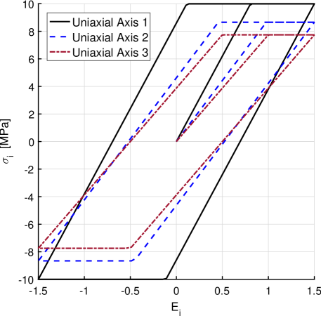
Figure 2: Cyclic tension-compression uniaxial tests over orthotropy preferred directions. We represent by $\sigma_{i}$ and $E_{i}$ the uniaxial components of the Cauchy stress and the logarithmic strain in the test performed in axis $(i)$. Perfect plasticity case, i.e. $k=k_{0}=const$.

7 Conclusion

In this paper we have presented a novel framework for elastoplasticity at large strains. This framework, grounded in the multiplicative decomposition, naturally solves the “rate issue”; i.e. the flow rule is naturally obtained in terms of a corrector elastic strain rate which simply results to be a partial contribution to the total rate of such strain, exactly as in the small strain theory. The new approach results in essentially the same type of equations in small strains and in large strains, and whether the latter are integrated in the intermediate or in the spatial configurations. The continuum framework also naturally results in the typical two stages of the algorithmic integration of elastoplastic equations: the trial elastic predictor and the plastic corrector. Hence the development of integration algorithms employing this proposal is straightforward by the direct use of the backward-Euler integration rule over the corrector logarithmic strain rate without explicitly employing exponential mappings. The large strain formulation, being simpler than most proposals in the literature, is also general, meaning that it is not restricted to moderate elastic strains and it is not restricted to isotropy. Furthermore, as shown in the manuscript, there is no need to perform any dissipation hypothesis in the plastic spin, which remains uncoupled and completely independent of the integration of the symmetric flow. The present formulation may be equally employed in metal plasticity or in the plastic behavior of soft materials.

References

References

- [1] JC Simó. Numerical analysis and simulation of plasticity. Handbook of numerical analysis, 183–499, 1998.
- [2] M Kojić, KJ Bathe. Inelastic analysis of solids and structures. Berlin: Springer, 2005.
- [3] J Lubliner. Plasticity theory. Courier Corporation, 2008.
- [4] JC Simó, TJR Hughes. Computational inelasticity. New York: Springer, 1998.
- [5] M Miñano, MA Caminero, FJ Montáns. On the numerical implementation of the Closest Point Projection algorithm in anisotropic elasto-plasticity with nonlinear mixed hardening. Finite Elements in Analysis and Design, 121, 1-17, 2016
- [6] AV Shutov, J Ihlemann. Analysis of some basic approaches to finite strain elasto-plasticity in view of reference change. International Journal of Plasticity, 63, 183–197, 2014.
- [7] ML Wilkins. Calculation of elastic-plastic flow. In: B Alder, S Fernback, M Rotenberg (eds.), Methods of Computational Physics, 3, New York: Academic Press, 1964.
- [8] G Maenchen, S Sacks. The tensor code. In: B Alder, S Fernback, M Rotenberg (eds.), Methods of Computational Physics, 3, New York: Academic Press, 1964.
- [9] RD Krieg, SW Key. Implementation of a time dependent plasticity theory into structural computer programs. In: JA Stricklin, KJ Saczlski (eds.), Constitutive Equations in Viscoplasticity: Computational and Engineering Aspects, AMD-20, New York, ASME, 1976.
- [10] C Truesdell, W Noll. The nonlinear field theories. In: Handbuch der Physik 111/3, Berlin: Springer, 1965.
- [11] HD Hibbitt, PV Marcal, JR Rice. A finite element formulation for problems of large strain and large displacement. International Journal of Solids and Structures, 6(8), 1069–1086, 1970.
- [12] RM McMeeking, JR Rice. Finite-element formulations for problems of large elastic-plastic deformation. International Journal of Solids and Structures 11(5), 601–616, 1975.
- [13] SW Key, RD Krieg. On the numerical implementation of inelastic time dependent and time independent, finite strain constitutive equations in structural mechanics. Computer methods in applied mechanics and engineering 33(1), 439–452, 1982.
- [14] LM Taylor, EB Becker. Some computational aspects of large deformation, rate-dependent plasticity problems. Computer methods in applied mechanics and engineering, 41(3), 251–277, 1983.
- [15] JC Simó, KS Pister. Remarks on rate constitutive equations for finite deformation problems: computational implications. Computer Methods in Applied Mechanics and Engineering, 46(2), 201–215, 1984.
- [16] M Kojić, KJ Bathe. Studies of finite element procedures—Stress solution of a closed elastic strain path with stretching and shearing using the updated Lagrangian Jaumann formulation. Computers & Structures, 26(1), 175–179, 1987.
- [17] TJ Hughes, J Winget. Finite rotation effects in numerical integration of rate constitutive equations arising in large-deformation analysis. International journal for numerical methods in engineering, 15(12), 1862–1867, 1980.
- [18] PM Pinsky, M Ortiz, KS Pister. Numerical integration of rate constitutive equations in finite deformation analysis. Computer Methods in Applied Mechanics and Engineering, 40(2), 137–158, 1983.
- [19] H Xiao, OT Bruhns, A Meyers. Hypo-elasticity model based upon the logarithmic stress rate. Journal of Elasticity, 47(1), 51–68, 1997.
- [20] OT Bruhns, H Xiao, A Meyers. Self-consistent Eulerian rate type elasto-plasticity models based upon the logarithmic stress rate. International Journal of Plasticity, 15(5), 479–520, 1999.
- [21] H Xiao, OT Bruhns, A Meyers. The choice of objective rates in finite elastoplasticity: general results on the uniqueness of the logarithmic rate. Proc. R. Soc. Lond. A, 456(2000), 1865–1882, 2000.
- [22] T Brepols, IN Vladimirov, S Reese. Numerical comparison of isotropic hypo-and hyperelastic-based plasticity models with application to industrial forming processes. International Journal of Plasticity, 63, 18–48, 2014.
- [23] JP Teeriaho. An extension of a shape memory alloy model for large deformations based on an exactly integrable Eulerian rate formulation with changing elastic properties. International Journal of Plasticity, 43, 153–176, 2013.
- [24] H Xiao, XM Wang, ZL Wang, ZN Yin. Explicit, comprehensive modeling of multi-axial finite strain pseudo-elastic SMAs up to failure. International Journal of Solids and Structures, 88, 215–226, 2016.
- [25] Y Zhu, G Kang, C Yu, LH Poh. Logarithmic rate based elasto-viscoplastic cyclic constitutive model for soft biological tissues. Journal of the mechanical behavior of biomedical materials, 61, 397–409, 2016.
- [26] R Rubinstein, SN Atluri. Objectivity of incremental constitutive relations over finite time steps in computational finite deformation analyses. Computer Methods in Applied Mechanics and Engineering, 36(3), 277–290, 1983.
- [27] JH Argyris, JS Doltsinis. On the large strain inelastic analysis in natural formulation Part I: Quasistatic problems. Computer Methods in Applied Mechanics and Engineering, 20(2), 213–251, 1979.
- [28] JC Simó, M Ortiz. A unified approach to finite deformation elastoplastic analysis based on the use of hyperelastic constitutive equations. Computer methods in applied mechanics and engineering, 49(2), 221–245, 1985.
- [29] G Gabriel, KJ Bathe. Some computational issues in large strain elasto-plastic analysis. Computers & structures, 56(2), 249–267, 1995.
- [30] AE Green, PM Naghdi. A general theory of an elastic-plastic continuum. Archive for rational mechanics and analysis, 18(4), 251–281, 1965.
- [31] EH Lee. Elastic-plastic deformations at finite strains. Journal of Applied Mechanics, 36, 1–6, 1969.
- [32] C Miehe. A formulation of finite elastoplasticity based on dual co-and contra-variant eigenvector triads normalized with respect to a plastic metric. Computer Methods in Applied Mechanics and Engineering, 159(3), 223–260, 1998.
- [33] P Papadopoulos, J Lu. A general framework for the numerical solution of problems in finite elasto-plasticity. Computer Methods in Applied Mechanics and Engineering, 159(1), 1–18, 1998.
- [34] P Papadopoulos, J Lu. On the formulation and numerical solution of problems in anisotropic finite plasticity. Computer Methods in Applied Mechanics and Engineering, 190(37), 4889–4910, 2001.
- [35] C Miehe, N Apel, M Lambrecht. Anisotropic additive plasticity in the logarithmic strain space: modular kinematic formulation and implementation based on incremental minimization principles for standard materials. Computer Methods in Applied Mechanics and Engineering, 191(47), 5383–5425, 2002.
- [36] J Löblein, J Schröder, F Gruttmann, F. Application of generalized measures to an orthotropic finite elasto-plasticity model. Computational materials science, 28(3), 696–703, 2003.
- [37] C Sansour, W Wagner. Viscoplasticity based on additive decomposition of logarithmic strain and unified constitutive equations: Theoretical and computational considerations with reference to shell applications. Computers & structures, 81(15), 1583–1594, 2003.
- [38] MH Ulz. A Green–Naghdi approach to finite anisotropic rate-independent and rate-dependent thermo-plasticity in logarithmic Lagrangean strain–entropy space. Computer Methods in Applied Mechanics and Engineering, 198(41), 3262–3277, 2009.
- [39] AE Green, PM Naghdi. Some remarks on elastic-plastic deformation at finite strain. International Journal of Engineering Science, 9(12), 1219–1229, 1971.
- [40] I Schmidt. Some comments on formulations of anisotropic plasticity. Computational materials science, 32(3), 518–523, 2005.
- [41] M Itskov. On the application of the additive decomposition of generalized strain measures in large strain plasticity. Mechanics research communications, 31(5), 507–517, 2004.
- [42] P Neff, ID Ghiba. Loss of ellipticity for non-coaxial plastic deformations in additive logarithmic finite strain plasticity. International Journal of Non-Linear Mechanics, 81, 122–128, 2016.
- [43] GI Taylor. Analysis of plastic strain in a cubic crystal. In: JM Lessels (ed.), Stephen Timoshenko 60th Anniversary Volume, New York: Macmillan, 1938.
- [44] JR Rice. Inelastic constitutive relations for solids: an internal-variable theory and its application to metal plasticity. Journal of the Mechanics and Physics of Solids, 19(6), 433–455, 1971.
- [45] J Mandel. Thermodynamics and plasticity. In: JJ Delgado Domingers, NR Nina, JH Whitelaw (eds.), Foundations of Continuum Thermodynamics, London: Macmillan, 283–304, 1974.
- [46] JC Simo. A framework for finite strain elastoplasticity based on maximum plastic dissipation and the multiplicative decomposition: Part I. Continuum formulation. Computer methods in applied mechanics and engineering, 66(2), 199–219, 1988.
- [47] JC Simo, C Miehe. Associative coupled thermoplasticity at finite strains: formulation, numerical analysis and implementation. Computer Methods in Applied Mechanics and Engineering, 98(1), 41–104, 1992.
- [48] L Anand. On H. Hencky’s approximate strain-energy function for moderate deformations. Journal of Applied Mechanics, 46(1), 78–82, 1979.
- [49] L Anand. Moderate deformations in extension-torsion of incompressible isotropic elastic materials. Journal of the Mechanics and Physics of Solids, 34(3), 293–304, 1986.
- [50] JR Rice. Continuum mechanics and thermodynamics of plasticity in relation to microscale deformation mechanisms. In: Constitutive Equations in Plasticity, Cambridge: Massachusetts Institute of Technology Press, 23–79, 1975.
- [51] WD Rolph, KJ Bathe. On a large strain finite element formulation for elasto-plastic analysis. In: KJ Willam (ed.), Constitutive equations: macro and computational aspects, AMD, New York: ASME, 131–147, 1984.
- [52] G Weber, L Anand. Finite deformation constitutive equations and a time integration procedure for isotropic, hyperelastic-viscoplastic solids. Computer Methods in Applied Mechanics and Engineering, 79(2), 173–202, 1990.
- [53] AL Eterovic, KJ Bathe. A hyperelastic-based large strain elasto-plastic constitutive formulation with combined isotropic-kinematic hardening using the logarithmic stress and strain measures. International Journal for Numerical Methods in Engineering, 30(6), 1099–1114, 1990.
- [54] D Perić, DRJ Owen, ME Honnor. A model for finite strain elasto-plasticity based on logarithmic strains: Computational issues. Computer Methods in Applied Mechanics and Engineering, 94(1), 35–61, 1992.
- [55] A Cuitiño, M Ortiz. A material-independent method for extending stress update algorithms from small-strain plasticity to finite plasticity with multiplicative kinematics. Engineering computations, 9(4), 437–451, 1992.
- [56] JC Simó. Algorithms for static and dynamic multiplicative plasticity that preserve the classical return mapping schemes of the infinitesimal theory. Computer Methods in Applied Mechanics and Engineering, 99(1), 61–112, 1992.
- [57] OT Bruhns. The multiplicative decomposition of the deformation gradient in plasticity—origin and limitations. In: H Altenbach, T Matsuda, D Okumura (eds.), From Creep Damage Mechanics to Homogenization Methods, Advanced Structured Materials 64, 37–66, Springer International Publishing, 2015.
- [58] C Eckart. The thermodynamics of irreversible processes. IV. The theory of elasticity and anelasticity. Physical Review, 73(4), 373–382, 1948.
- [59] JF Besseling. A thermodynamic approach to rheology. In: H Parkus, LI Sedov (eds.), Irreversible Aspects of Continuum Mechanics and Transfer of Physical Characteristics in Moving Fluids, Vienna: Springer, 16–53, 1968.
- [60] AI Leonov. Nonequilibrium thermodynamics and rheology of viscoelastic polymer media. Rheologica acta, 15(2), 85-98, 1976.
- [61] MB Rubin, O Vorobiev, E Vitali. A thermomechanical anisotropic model for shock loading of elastic-plastic and elastic-viscoplastic materials with application to jointed rock. Computational Mechanics, 1–22, 2016.
- [62] MÁ Caminero, FJ Montáns, KJ Bathe. Modeling large strain anisotropic elasto-plasticity with logarithmic strain and stress measures. Computers & Structures, 89(11), 826–843, 2011.
- [63] S Chatti, A Dogui, P Dubujet, F Sidoroff. An objective incremental formulation for the solution of anisotropic elastoplastic problems at finite strain. Communications in numerical methods in engineering, 17(12), 845–862, 2001.
- [64] CS Han, K Chung, RH Wagoner, SI Oh. A multiplicative finite elasto-plastic formulation with anisotropic yield functions. International Journal of Plasticity, 19(2), 197–211, 2003.
- [65] B Eidel, F Gruttmann. Elastoplastic orthotropy at finite strains: multiplicative formulation and numerical implementation. Computational Materials Science, 28(3), 732–742, 2003.
- [66] A Menzel, M Ekh, K Runesson, P Steinmann. A framework for multiplicative elastoplasticity with kinematic hardening coupled to anisotropic damage. International Journal of Plasticity, 21(3), 397–434, 2005.
- [67] C Sansour, I Karšaj, J Sorić. A formulation of anisotropic continuum elastoplasticity at finite strains. Part I: Modelling. International journal of plasticity, 22(12), 2346–2365, 2006.
- [68] FJ Montáns, KJ Bathe. Towards a model for large strain anisotropic elasto-plasticity. In: E Oñate, R Owen (eds.), Computational Plasticity, Netherlands: Springer, 13–36, 2007.
- [69] DN Kim, FJ Montáns, KJ Bathe. Insight into a model for large strain anisotropic elasto-plasticity. Computational Mechanics, 44(5), 651–668, 2009.
- [70] IN Vladimirov, MP Pietryga, S Reese. Anisotropic finite elastoplasticity with nonlinear kinematic and isotropic hardening and application to sheet metal forming. International Journal of Plasticity, 26(5), 659–687, 2010.
- [71] J Mandel. Plasticité Classique et Viscoplasticité. Course held at the Department of Mechanics of Solids, New York: Springer, 1972.
- [72] M Latorre, FJ Montáns. Stress and strain mapping tensors and general work-conjugacy in large strain continuum mechanics. Applied Mathematical Modelling, 40(5), 3938–3950, 2016.
- [73] J Lubliner. Normality rules in large-deformation plasticity. Mechanics of Materials, 5(1), 29–34, 1986.
- [74] M Latorre, FJ Montáns. On the interpretation of the logarithmic strain tensor in an arbitrary system of representation. International Journal of Solids and Structures, 51(7), 1507–1515, 2014.
- [75] J Bonet, RD Wood. Nonlinear continuum mechanics for finite element analysis. Second Edition, Cambridge University Press, 2008.
- [76] M Latorre, FJ Montáns. Anisotropic finite strain viscoelasticity based on the Sidoroff multiplicative decomposition and logarithmic strains. Computational Mechanics, 56(3), 503–531, 2015.
- [77] M Pastor, OC Zienkiewicz, AHC Chan. Generalized plasticity and the modelling of soil behavior. International Journal for Numerical and Analytical Methods in Geomechanics, 14(3), 151-190, 1990.
- [78] RI Borja. Plasticity–Modeling and Computation. Springer, Berlin 2013.
- [79] FJ Montáns, JM Benítez, MÁ Caminero. A large strain anisotropic elastoplastic continuum theory for nonlinear kinematic hardening and texture evolution. Mechanics Research Communications, 43, 50–56, 2012.
- [80] A Menzel, P Steinmann. On the spatial formulation of anisotropic multiplicative elasto-plasticity. Computer Methods in Applied Mechanics and Engineering, 192(31), 3431–3470, 2003.
- [81] D Perić, W Dettmer. A computational model for generalized inelastic materials at finite strains combining elastic, viscoelastic and plastic material behaviour. Engineering Computations, 20(5/6), 768–787, 2003.
- [82] S Reese, S Govindjee. A theory of finite viscoelasticity and numerical aspects. International journal of solids and structures, 35(26), 3455–3482, 1998.
- [83] DW Holmes, JG Loughran. Numerical aspects associated with the implementation of a finite strain, elasto-viscoelastic–viscoplastic constitutive theory in principal stretches. International journal for numerical methods in engineering, 83(3), 366–402, 2010.
- [84] FJ Montáns, KJ Bathe. Computational issues in large strain elasto-plasticity: an algorithm for mixed hardening and plastic spin. International Journal for Numerical Methods in Engineering, 63(2), 159–196, 2005.
- [85] AS Shutov, R Landgraf, J Ihlemann. An explicit solution for implicit time stepping in multiplicative finite strain viscoelasticity. Computer Methods in Applied Mechanics and Engineering, 256, 213–225, 2013.
- [86] M Latorre, FJ Montáns. What-You-Prescribe-Is-What-You-Get orthotropic hyperelasticity. Computational Mechanics, 2014, 53(6), 1279–1298.