CAVAthesis

Abstract

The brain in complex animals is organized in different areas, such as visual areas, motor areas etc., which are believed to be responsible for specific functions. Each area can have in turn its own organization, but for all areas it is believed that their functions rely on the dynamics of networks of neurons rather than on single neurons. On the other hand, the network dynamics reflect and arise from the integration and coordination of the activity of populations of single neurons. Understanding how single-neurons and neural-circuits dynamics complement each other to produce brain functions is thus of paramount importance.

LFPs and EEGs are good indicators of the dynamics of mesoscopic and macroscopic populations of neurons, while microscopic-level activities can be documented by measuring the membrane potential, the synaptic currents or the spiking activity of individual neurons. How can we combine the information coming from microscopic, mesoscopic and macroscopic levels to get better insights about the relationships between single-neuron activity and the state of neural circuits? How can we model the relationship between these two levels? How can we optimally analyze concurrent recordings at multiple scales to gain insights on the relationship between macroscopic/mesoscopic and microscopic brain dynamics?

In this thesis we develop mathematical modelling and mathematical analysis tools that can help the interpretation of joint measures of neural activity at microscopic and mesoscopic or macroscopic scales. In particular, we develop network models of recurrent cortical circuits that can clarify the impact of several aspects of single-neuron dynamics (that depend on the details of synaptic dynamics) on the activity of the whole neural population (i.e., at the mesoscopic level). We then develop statistical tools to characterize the relationship between the action potential firing of single neurons and mass signals. We apply these latter analysis techniques to joint recordings of the firing activity of individual cell-type identified neurons and mesoscopic (i.e., LFP) and macroscopic (i.e., EEG) signals in the mouse neocortex. We identified several general aspects of the relationship between cell-specific neural firing and mass circuit activity, providing for example general and robust mathematical rules which infer single-neuron firing activity from mass measures such as the LFP and the EEG.

chapter

A computational investigation of the relationships
between single-neuron and network dynamics
in the cerebral cortex
Stefano Cavallari

Advisor: Prof. Stefano Panzeri
Co-advisor: Dr. Alberto Mazzoni

A dissertation submitted in partial fulfillment

of the requirements for the degree of

Doctor of Philosophy (Ph.D.)

Doctoral School on “Life and Humanoid Technologies”
Doctoral Course on “Robotics, Cognition and Interaction Technologies”
April 2015
XXVII Cycle

"The brain is wider than the sky,
For, put them side by side,
The one the other will include
With ease, and you beside.

The brain is deeper than the sea,
For, hold them, blue to blue,
The one the other will absorb,
As sponges, buckets do.

The brain is just the weight of God,
For, lift them, pound for pound,
And they will differ, if they do,
As syllable from sound."

Emily Dickinson, 1862

Abbreviations

BMI	Brain Machine Interface
COBN	Conductance-Based Network
CUBN	Current-Based Network
EEG	Electroencephalography
fMRI	Functional Magnetic Resonance Imaging
FR	Firing Rate
GLM	General Linear Model
LIF	Leaky Integrate-and-Fire
LFP	Local Field Potential
MP	Membrane Potential
MUA	Multi-Unit Activity
NMSD	Normalized Mean Squared Distance
OU	Ornstein-Uhlenbeck
PSP	Post Synaptic Potential
PV-pos	Parvalbumin-positive interneuron
SOM-pos	Somatostatin-positive interneuron
spk	Spike times
SUA	Single-Unit Activity

Chapter 0 Introduction

In the first hundred years of neuroscience, many influential studies that shaped our current understanding of brain function were performed by recording and considering the response properties of single neurons in isolation. Examples of this progress are for the classic work of Vernon Mountcastle or of David Huebel and Thisten Wiesel on the receptive field and stimulus tuning properties of neurons in different sensory modalities (Mountcastle, 1957; Talbot et al., 1968; Mountcastle, 1978; Hubel & Wiesel, 1959, 1962; Wiesel et al., 1963; Hubel & Wiesel, 1968) or the work of Michael Brecht and colleagues on the behavioral effect of stimulating individual neurons (Houweling & Brecht, 2008). However, considering each neuron in isolation can only lead us so far. No neuron is an island. In recent studies, the idea of point neurons performing a function is gradually being replaced by the conceptual framework of considering neurons as part of the circuits they belong to.

Neurons belong to microcircuits, not all elements of which are necessarily selective to sensory stimulus, and not all activations within the microcircuits imply a direct control of the neuron by the sensory stimulus, as it would be the case in feedforward processing. Feedforward inputs to cortical microcircuits are typically weak, and there is strong recurrent excitation and inhibition whose balance - which is obviously critical for circuit dynamics - may depend on the external input as well as on neuromodulation (Logothetis, 2008). Thus the activity of a neuron can only be understood in the context of the state of the microcircuit, mesoscopic and macroscopic circuits it belongs to (Panzeri et al., 2015). Given that most brain functions likely arise from the concerted operation of many microscopic and macroscopic circuits, even very dense recordings from a single structure can only get us so far.

The alternative to single-neuron recording, which is the dominating one for studying neural mechanisms of cognition in humans, is to use tools such as fMRI or EEG/MEG to collect macroscopic measures of massed neural action over large regions (potentially, the whole brain). This has the clear advantage of being able to capture concerted relationships between macroscopic structures. However, the linkage between microscopic neuronal activity and the measured massed action at each site is immensely complex. Take for example EEG. The typical integration area of an EEG electrode contains several million neurons, a few tens of billion synapses, tens of km of dendrites and hundreds of km of axons. These numbers by themselves suggest the difficulty of drawing analogies between mass measures and microscopic neural activity. In addition, the organization of microconnectivity within the microcircuit (or EEG integration area) leads (as discussed above) to state-dependent dynamics (Douglas et al., 1989; Douglas & Martin, 2004). This means that mesoscopic and macroscopic massed neural dynamics can in principle arise from a large number of states or different circuit operations. This in turn implies that the neural interpretation of massed noninvasive methodologies may not be possible without concurrent electrical measurements of activity of single neurons or small populations thereof (Panzeri et al., 2015).

Because of the above reasons, recent experimental efforts have been aimed at the simultaneous recording of microscopic and mesoscopic-macroscopic brain activity. Several recent studies reported new observations of the relationships between the spiking dynamics of a few neurons and of mesoscopic and macroscopic circuits they belong to (Schwartz et al., 2006; Whittingstall & Logothetis, 2009; Rasch et al., 2008, 2009; Nauhaus et al., 2009; Okun et al., 2010; Zanos et al., 2012; Waldert et al., 2013; Hall et al., 2014), revealing for example that the information carried by single neurons is state-dependent (Harris & Thiele, 2011) and it can only be read out when single-neuron spikes are referred to indicators of microcircuit state such as the phase of LFPs (Montemurro et al., 2008; Kayser et al., 2009; Mazzoni et al., 2011; Panzeri et al., 2015). In addition, other studies have begun to use simultaneous recordings of the local activity of small neural populations together with large-scale measures of mass activity in multiple regions, and have given already important insights into the relationship between local and global brain dynamics. For example, one study (Canolty et al., 2010) used simultaneous recordings of spiking activity and LFPs from multiple brain regions to reveal the important role of phase coordination among oscillations in different regions for the selective recruitment of cell assemblies. Another study (Logothetis et al., 2012) used concurrent electrophysiological measures and whole-brain fMRI to reveal the patterns of whole-brain activity that happen in correspondence to the firing of high-frequency sharp wave ripple events in the hippocampus.

These new simultaneous recordings of signals at different scales hold the key to relate microcircuit dynamics to massed neural activity and to the interrelationships among macroscopic networks. However, we still lack the appropriate mathematical tools to properly analyze and interpret these recordings. In particular, we need better modeling tools to relate single-neuron synaptic and spiking dynamics to the dynamics of the whole circuit. We also need better analytical tools to describe the empirical relationships between the microscopic activity of specific cell types in cortex and the macroscopic or mesoscopic circuit activation. In this thesis, we make progress along both these directions.

The work presented in this thesis is organized as follows.

In the next chapter, we begin by summarizing the main concepts of computational neuroscience that we used to develop this work (i.e., LIF network models, mutual information and Wiener kernel methods) to give the opportunity to readers without specialist background on mathematical neuroscience to acquire the basic tools that will help the understanding of the research presented in successive chapters.

In chapter 2, we describe a new neural network modelling framework that permits the understanding of the impact of specific details of synaptic dynamics onto mesoscopic-level circuit activity. First we develop a new algorithm for comparing quantitatively and fairly how different assumptions (i.e., mathematical expressions) about synaptic dynamics affect circuit-level activity. Previous studies have compared the effects of different choices of synaptic models mainly at the single-neuron level or choosing parameters for network-dynamics comparison in a rather arbitrary way, whereas we introduce a rigorous framework to perform such comparison. By applying this formalism to the study of the dynamics of recurrent networks, we find that the network-scale first order statistics (population FR and spectrum of the network oscillations) are robust to the changes in the single-neuron synaptic properties, while both the correlation properties of neural population interactions and the modulation of network oscillations by external inputs strongly depend on the choice of the synaptic model (Cavallari et al., 2014).

In chapter 3, we first develop - and then apply to data - new mathematical tools for the analysis of the relationship between single-neuron spiking activity and mass signals (EEG or LFP). We apply these tools to simultaneous recordings of LFPs and EEGs together with the firing activity of identified classes of neurons during slow wave oscillations. We find that the linear component of the relationship between single-neuron activity and mass signals is remarkably stable across cells and animals, allowing a blind estimation of the mass signals from the spiking activity (both of excitatory and inhibitory neurons) and vice versa. We also observe that the single-unit activity tends to prevent changes in both the LFP and EEG signals.

Finally, in chapter 4, we summarized the results presented in the previous chapters and discussed their implications, as well as further questions arising from this work. We concluded by describing very interesting and promising directions for further investigations.

Chapter 1 Theoretical framework

The brain is likely the most complex system in the universe, and we are still far away from a general theory able to explain from first principles the way it works. In absence of a first-principles general theory, it has been however possible to make progress by identifying mechanisms at multiple spatial and temporal scales that likely influence brain dynamics, and then building quantitative mathematical models of these mechanisms. These models can in turn be compared to data and help to validate quantitatively and refine initial hypothesis on the relationship between the brain’s biophysics and the brain’s function. The effort on mathematical modelling of neurons and neural networks has been vast (for recent books, see Dayan & Abbott (2001); Quiroga & Panzeri (2013); Izhikevich (2007); Gerstner et al. (2014)) and cannot be reviewed in a single thesis.

In this section, however, we introduce a small set of elements of the conceptual and mathematical formulation of neural function (Bear et al., 2007) and of the main features of the (single-neuron and network) models (Dayan & Abbott, 2001) that we will use to investigate the relationship between network dynamics and single-neuron activity (see chapter 2). We hope that this short introduction will help readers without a specialist background to navigate through our original research, which we will present in the next chapters.

1 Modelling neurons and neural circuits

1 Introduction

The brains of all species composed primarily of two broad classes of cells: neurons and glial cells. Glial cells come in several types, and perform a number of critical functions, including structural support, metabolic support, insulation, and guidance of development, neurons, however, are usually considered the most important cells in the brain (Kandel et al., 1999) and in this work we will focus only on the neuronal activity.

The brain (like any biological systems) can be investigated with many different instruments (e.g. microelectrodes, calcium-imaging, fMRI, etc.) and each of them take pictures of the brain activity from a different prospective (and on a different scale). It is similar to what happen in Physics with the description of a physical system in different reference frames, but in neuroscience we are still faraway from knowing the transformation laws to move from a reference system to another. Our point of view to investigate the brain activity (our "reference system") it is represented by the electrical properties/activity of the neurons and of networks of neurons measured through microelectrodes or glass pipette. Therefore we are going to introduce a simple way to model the electrical properties of the neurons. In particular, we will use the electrical circuits theory to model the neurons and their networks (with some ad hoc assumptions to model the action potential), so, in the end, we will describe the neural networks as specific electrical circuits. Indeed the ingredients we will adopt to build the model are electric charges, electric potentials, capacitors, resistance, electric currents, etc… This is also the most natural choice because

1. The neurons exchange action potentials, which are electric potential

2. The experimental data we will use to test our models come from recordings of electric potentials

The neurons communicate each other through electrical signals that travel across the neuronal structures. The electrical signals are i.e., positive ons (like Ca²⁺, K⁺, Na⁺, Cl^-) that move driven by an electric potential generated by an inhomogeneous spatial displacement of positive and negative charges (ions). The neuronal structure that allows this separation of positive and negative charge (needed to generate the electrical potential) is the cell membrane.

The cell membrane is a lipid bilayer 3 to 4 nm thick that is essentially impermeable to most charged molecules. This insulating feature causes the cell membrane to act as a capacitor where the two electrical plates are given by the internal and external surfaces of the membrane. The (membrane) potential is precisely the difference between the electrical potentials measured on these two surfaces of the membrane. Most of the time, there is an excess concentration of negative charge inside a neuron. By convention, the potential of the extracellular fluid outside a neuron is defined to be zero, therefore, when a neuron is at rest (that is the net flow of current across the cell membrane is zero) the potential is negative with a value around -65 mV.

The membrane is embedded with many ion-conducting channels (usually highly selective, see figure 1) which affect in a dynamic-dependent way the ionic permeability of the membrane (that overall increases of about 10,000 times with respect to a pure lipid bilayer). Indeed the movement of ionic charges and the generation and transmission of action potentials in the neurons are ruled by a lot of complex biological mechanisms which ultimately determine the opening and the closing of the ionic channels: the cell membrane actively shapes the flow of the ionic currents. Therefore the electric signals spreading across neural networks is different both in the way it travels and in composition (it is a ionic current, not a current of free electrons) with respect to a current of free electrons flowing in a conductive materials. Furthermore the membrane contains pumps for selected ions whose role is to expend energy to maintain the difference in the ion concentrations between the inner and the outer part of the cell.

Figure 1: Schematic diagram of two ion channels embedded in a section of lipid bilayer. The ion channels are about 10 nm long. (Source: Dayan & Abbott, 2001)

In summary, the conductive properties of the channels can be affected by many factors such as:

• the membrane potential

• the intracellular concentration of various intracellular messengers (e.g. Ca²⁺-dependent channels)

• the extracellular concentration of neurotransmitters

• the presence of the ionic pumps

2 Single-compartment models

The membrane potential measured at different places within a neuron can take different values. The single-compartment models are single-neuron models where the entire neuron is described with a single membrane potential, $V$. Therefore this approximation assumes that the neuron has a (relatively) uniform membrane potential across their surfaces. In general this may looks a rough approximation, and a way to evaluate how good it is at the single-neuron level is to compute the electrotonic distance (Koch, 2004), nevertheless, depending on the dynamics and the scale we are modeling, there are many situations where the spatial variations in the membrane potential inside a neuron is not thought to play an important function.

We have mentioned that there is typically an excess of negative charge on the inside surface of the cell membrane of a neuron, and a balancing positive charge on its outside surface (see figure 2). In this arrangement we can model the neuron as a spherical capacitor (whose potential is kept constant by the ionic pumps) and by introducing the capacitance, $C_{m}$, we can use the standard equation for a capacitor to relate the variation of the total charge between the internal and external surfaces of the membrane, $Q$, to the variation of the potential: $Q=C_{m}V$ . By doing the time derivative of the previous equation we can determine how much current is required to change the membrane potential at a given rate:

$$C_{m}\frac{dV}{dt}=\frac{dQ}{dt}.$$ (1)

This is the basic relationship that determine the membrane potential for a single-compartment model. The specific membrane capacitance is approximately the same for all neurons: $c_{m}\approx 10$nF/mm², while the surface area, $A$, is usually between 0.01 and 0.1 mm², so the capacitance, $C_{m}$, is typically in the range 0.1 to 1 nF.

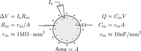
Figure 2: The capacitance and the resistance of a neuron in the single-compartment model. Typical values of specific membrane capacitance and resistance, $c_{m}$ and $r_{m}$, are given. In the equation relating the current and the potential flowing through the membrane resistance, $R_{m}$, the restriction to small currents ΔV is needed to have $R_{m}$ constant over the range ΔV, as assumed by the Ohm’s law. (Source: Dayan & Abbott, 2001)

The neuron also shows features that can be modeled by a resistance, indeed when a current, $I_{e}$, is injected into a neuron through an electrode, see figure 2, the relationship between the current and the variation of the potential, ΔV, can be modeled by a membrane or input resistance, $R_{m}$. Analogously, the membrane resistance determines how much current is required to keep the potential fix to a given value different from its resting value, while the capacitance of a neuron determines how much current is required to make the membrane potential change at a given rate (see equation 1). The specific membrane resistance of a neuron at rest is around 1 MΩ mm², but its value is much more variable than the specific membrane capacitance.

The right-hand side of equation 1 is given by the total amount of current entering the neuron and it can be split in two main components: the physiological currents, $i_{m}$, (flowing through all the membrane and the synapses) and the experimentally injected currents, $I_{e}$ (if it is present). The former are usually in units of current per unit area (to facilitate comparisons between neurons of different sizes), while the latter is the total current injected through the electrode, therefore, putting all together we can rewrite the equation 1 as:

$$C_{m}\frac{dV}{dt}=-i_{m}(t)+\frac{I_{e}(t)}{A},$$ (2)

where the sign of $i_{m}$ is negative because, by convention, membrane currents are defined as positive when positive ions flow outward the neuron (i.e., membrane-hyperpolarizing currents are positive) and negative when positive ions flow inward the neuron. On the other hand, when the current enters through an electrode the signs of the currents (i.e. electrode-depolarizing currents are positive).

3 Nernst equation

The movement of ions through the channels of the membrane is due to two distinct effects: electric forces and thermal diffusion. Indeed the ionic pumps maintain an inhomogeneous concentration of charges (in particular Cl^-, Na⁺ e Ca²⁺are more concentrated outside, while K⁺inside) between the interior and the exterior of the cells, therefore, both the electric force (positive ions will be attracted towards negative potentials and vice versa) and the thermal energy (which tends to homogeneously diffuse the ions) act on the ions. We can characterize the balance between these two contributes by means of "equilibrium potentials". The equilibrium potential, $E$, is indeed defined as the membrane potential at which current flow due to electric forces cancels the diffusive flow and there is not net movement of charges through the cell membrane. The equilibrium potential is a function of the state of the neuron and of to the considered and active channels. For example, when the neuron is at rest $E$ is around -65 mV and it results by summing contributions from all the active channels of the neuron.

In the simplest case where the channel $x$ conducts only one type of ion, $x$, having electric charge $zq$ ($q$ is the charge of a proton), by using the Boltzmann distribution to evaluate the thermal energy and by equating the ionic flows due to the thermal and to the electric contributes, we obtain:

$$E_{x}=\frac{V_{T}}{z}ln\left(\frac{[outside]_{x}}{[inside]_{x}}\right),$$ (3)

where $[outside]_{x}$ and $[inside]_{x}$ are the values of the concentration of the ion $x$ respectively outside and inside the neuron. This is the Nernst equation, which allows to compute the equilibrium potential of a ionic channel (that allows only one type of ion to pass through it) $x$. In the table 1 are shown some typical values for the concentration of the four most important ions involved in the transmission of the neuronal signal.

Ion ($x$)	$[outside]_{x}$ (in mM)	$[inside]_{x}$ (in mM)	$[outside]:[inside]$	$E_{x}$ (at $37\mathrm{°}$C) [mV]
K+	5	100	1:20	-80
Na+	150	15	10:1	62
Ca2+	2	2$\cdot$10-4	104:1	123
Cl-	150	13	11.5:1	-65

Table 1: Approximated concentrations of the principal ions on both the membrane surfaces. (Adapted from Bear et al., 2007)

In our modeling framework each channel represents a conductance that allows the current to flow through the membrane. The direction of this current depends on the value of the membrane potential with respect to the equilibrium potential. Indeed a conductance $x$ with an equilibrium potential $E_{x}$ tends to move the membrane potential of the neuron toward the value $E_{x}$. When $V>E_{x}$ this means that positive current will flow outward, and when $V<E_{x}$, positive current will flow inward. This is the reason why the equilibrium potential is also called reversal potential and indicated by $V_{x}$. For example, looking at table 1 we see that Ca²⁺ and Na⁺conductances have positive reversal potentials, so they tend to depolarize a neuron, while the opposite normally happens with K⁺ channels.

4 Membrane currents

In order to model the membrane current flowing through the channel $x$, $i_{m,x}$, we make a first order approximation obtaining: $i_{m,x}(t)=g_{x}(t)(V(t)-V_{x})$. Summing over the different types of channels, we obtain the total membrane current (see equation 2):

$$i_{m}(t)=\underset{x}{\sum}g_{x}(t)(V(t)-V_{x}).$$ (4)

The term $(V(t)-V_{x})$ is called the driving force, because it is responsible for the intensity and the direction of the net movement of ions across the channel. In particular, the current flows in the direction that tends to minimize the driving force. The factor $g_{x}$ is the conductance per unit area due to the channel $x$ and it is in general a function of the time. Indeed much of the complexity and richness of neuronal dynamics arises because membrane conductances change over time (the channels can open and close depending on many factors, see section 1). Nevertheless some of the factors which contribute to the total membrane current can be treated as channels with a relatively constant synaptic conductance (e.g. the ionic pumps). In the simplest version of the model, they are grouped together into a single term called leakage current whose conductance is not a function of time. Therefore the total physiological current, $i_{m}$, can be split into two contributes:

$$i_{m}(t)=i_{leak}(t)+\underset{x}{\sum}i_{x}^{active}(t),$$ (5)

where

$$i_{leak}(t)=g_{leak}(V(t)-V_{leak}).$$ (6)

Since the leak conductance is time-independent, it is also called passive conductance to distinguish it from the variable conductances, which are termed active because they interact with the surrounding. Indeed they can be affected by both the state of the neuron (like the membrane potential value) and by the environment where the neuron is placed (like the concentration of a given ion). We can write the active currents as the product of a maximal conductance, $\bar{g}_{x}$, times an active probability, $s_{x}$, (that is the probability of finding the channel $x$ in an open and active state) in the following way:

$$i_{x}^{active}(t)=\bar{g}_{x}s_{x}(t)(V(t)-V_{x}),$$ (7)

where $V_{x}$ is the reversal potential of the channel and $s_{x}(t)$ a function that describes the channel dynamics.

5 Synaptic currents

A very important class of active conductances is given by the synapses. Indeed also the synapses can be modeled as conductances and depending on the value of their reversal potential they are termed excitatory or inhibitory. In particular, if a synaptic conductance has a reversal potential higher than the threshold for action potential generation, its activation will produce an increase of the membrane potential (that is a depolarization of the neuron) and the synapse is called excitatory. On the other hand when the reversal potential is lower than the threshold, its activation will hyperpolarize the neuron and the synapse is called inhibitory. This conductances cannot be efficiently modeled as constants, therefore, we write the synaptic currents as in equation 7:

$$i_{syn}(t)=\bar{g}_{syn}s_{syn}(t)(V(t)-V_{syn}),$$ (8)

where $V_{syn}$ is the reversal potential of the synapse $syn$ and $s_{syn}(t)$ is a function that models the synaptic dynamics. In particular, $s_{syn}(t)$ expresses the probability that the synaptic channel is open as a consequence of the arrival of an action potential. In order to write an explicit equation for $s_{syn}(t)$, we firstly introduce $P_{pre}$, which is the probability that the presynaptic neuron is activated by the arrival of an action potential at the synaptic terminal (and the neurotransmitter released in the synaptic cleft). When an action potential invades the presynaptic terminal, the transmitter concentration in the synaptic cleft rises extremely rapidly after vesicle release, remains at a high value for a period of duration $T$, and then falls rapidly to 0. Therefore, as a simple model of the presynaptic transmitter release, we assume that $P_{pre}$ is a square pulse (with pulses located at the spike times) of amplitude $T$.

Let’s assume now to model the opening an closing of the synaptic channel as two exponentials and introduce the following coefficients: $\alpha_{syn}$, which represents the opening rate of the synapse and $\beta_{syn}$, which is the closing rate of the synapse. In general these two coefficients are not constant and they can be function, for example, of the neurotransmitter concentration and of the membrane potential. In particular, since we are interested in the case where the synaptic channel is open when an action potential arrives, we take as effective opening rate the product $\alpha_{syn}P_{pre}$. The probability that a synaptic gate opens over a short time interval is proportional to the probability of finding the gate closed, $(1-s_{syn})$, multiplied by the opening rate $\alpha_{syn}P_{pre}$. Likewise, the probability that a synaptic gate closes during a short time interval is proportional to the probability of finding the gate open, $s_{syn}$, times the closing rate $\beta_{syn}$. Therefore, the equation for the probability that the synaptic channel is active is:

$$\frac{ds_{syn}}{dt}=\alpha_{syn}P_{pre}(t)(1-s_{syn}(t))-\beta_{syn}s_{syn}(t).$$ (9)

The solution for this equation depends on the spike train impinging on the neuron (through the presynaptic probability $P_{pre}$). The contribution to $s_{syn}$ of each post synaptic potential is given by the difference of two exponentials: one models the opening of the synaptic gates (that is the increase of $s_{syn}$ observed in correspondence of the arrival of an action potential) with time rise constant $\tau_{r}=1/\alpha_{syn}$, while the other exponential, which describes the closing of the synaptic gates with decay time $\tau_{d}=1/\beta_{syn}$, tends to vanish $s_{syn}$. $\alpha_{syn}$and $\beta_{syn}$ are obtained by fitting experimental data and typically $\tau_{r}$ is considerably smaller than $\tau_{d}$.

The synaptic currents can also be written in a simplified way by neglecting the dependence on the membrane potential $V(t)$:

$$i_{syn}(t)=j_{syn}s_{syn}(t),$$ (10)

where $j_{syn}$ is a constant (in units of current per unit area) which models the synaptic efficacy of the connections.

6 Leaky Integrate-and-Fire model

The leaky integrate-and-fire (LIF) model (Lapicque, 1907) is one of the simplest single-neuron model that includes the action potential generation. It is a single-compartment model with some ad hoc assumptions needed to introduce the action potential in the neuronal dynamic.

In particular, by substituting equation 6 into equation 2 we obtain a more explicit equation for the membrane potential of a single-compartment model:

$$c_{m}\frac{dV}{dt}=-g_{leak}(V(t)-V_{leak})-\underset{x}{\sum}g_{x}(t)(V(t)-V_{x})+\frac{I_{e}(t)}{A}.$$ (11)

In the simplest case the leak conductance, $g_{leak}$, can be approximated by the input conductance (that is the inverse of the input resistance, see figure 2): $g_{leak}=1/r_{m}.$ Therefore, by multiplying both sides by the specific membrane resistance, we obtain:

$$\tau_{m}\frac{dV}{dt}=-V(t)+V_{leak}-\underset{x}{\sum}\frac{g_{x}(t)}{g_{leak}}(V-V_{x})+R_{m}I_{e},$$ (12)

where $\tau_{m}=c_{m}r_{m}$ is a constant with units of time. It is called the membrane time constant and its typical values is between 10 and 100 ms. If there are not input currents (that is $g_{x}(t)=I_{e}=0$), the membrane potential exponentially decades to the value $V_{leak}$ with time constant $\tau_{m}$. Therefore $V_{leak}$ is the potential of the cell and it is also called the resting potential of the neuron. Equation 11 is the equation for the potential in a electrical circuit, called equivalent circuit, consisting of a capacitor and a set of variable and non variable resistors corresponding to the different channels of the membrane. Figure 3 shows the equivalent circuit for a generic one-compartment model.

Figure 3: On the right, it is shown the equivalent circuit for a single-compartment neuron model. On the left is represented the neuron (having surface area $A)$ with a single synapses and a current-injecting electrode. The equation 11 determines the evolution of the voltage in such a circuit. In particular, the circled $s$ indicates a synapse conductance (with reversal potential $E_{s}$), which is a function of the presynaptic neuron activity. Then we have the capacitance and the leak conductance, which are constant, and eventually a series of voltage dependent conductances (indicated by the circled v). The dots stand for possible additional membrane conductances or active currents (such as the spike-rate adaptation current). All the physiological active currents are included in the summation over the channels in the equation 11. (Source: Dayan & Abbott, 2001)

A neuron will typically fire an action potential when its action potential reaches a threshold value of about -55 to -50 mV. The generation and propagation of an action potential in a neuron are due to a cascade of events that are very complex and depends on a lot of variables. In the leaky integrate-and-fire model the description of these biophysical mechanisms is simply avoided: the subthreshold dynamics of the membrane potential follow the equation 12 and each time the membrane potential overcomes a fixed threshold, $V_{thresohld}$:

1. An action potential is instantaneously fired

2. The membrane potential is instantaneously set to the reset value, $V_{reset}$

3. The firing on another action potential is forbidden for a given absolute refractory period

Equation 12 combined with the three rules just stated define the leaky integrate-and-fire model of a neuron.

If there are not currents injected through an electrode ($I_{e}=0$) and all the active currents are due to synaptic inputs, equation 12 becomes:

$$\tau_{m}\frac{dV}{dt}=-V(t)+V_{leak}-\underset{syn}{\sum}\frac{\bar{g}_{syn}}{g_{leak}}s_{syn}(t)(V(t)-V_{syn}),$$ (13)

By using the simplified expression of the synaptic current, shown in equation 10, the equation for the membrane potential is:

$$\tau_{m}\frac{dV}{dt}=-V(t)+V_{leak}-\underset{syn}{\sum}\frac{j_{syn}}{g_{leak}}s_{syn}(t).$$ (14)

The difference between the single-neuron model described in equation 13 and the one in equation 14 relies on the synaptic current. Both of them are LIF neurons, but in the latter case, the dependence on the membrane potential is neglected and the synapses are termed “current-based”, while in the first case we have “conductance-based” synapses.

The leaky integrate-and-fire models is very useful to investigate, for example, how neurons integrate a high number of synaptic inputs. A major difference in the way neurons can respond to multiple synaptic inputs depends on the balance between excitatory and inhibitory inputs. In figure 4A the excitation is so strong, with respect to inhibition, to produce an average membrane potential (when action potential generation blocked) above the spiking threshold of the model. By turning on the spiking mechanism the neuron fires in a regular way (that is with a regular pattern of action potentials). In this case the timing of the action potentials is only weakly related to the temporal structure of the input currents, since it is mainly determined by the charging rate of the neuron, which depends on its membrane time constant. On the other hand, in figure 4B, the mean membrane potential (in absence of spiking mechanism) is below the threshold for action potential generation and the resulting spiking activity is irregular: action potentials are generated only when the fluctuations in the synaptic input are sufficiently strong to bring the membrane over the threshold. In this case the degree of variability of the spiking activity (than can be measured for example with the coefficient of variation of the interspike interval, CV ISI) is much higher than in the regular regime and it is more similar to the high degree of variability observed in the spiking patterns of in vivo recordings of cortical neurons. Furthermore in the irregular-firing mode the spiking activity reflect the temporal properties of fluctuation in the input currents. For these reason the irregular-firing mode is by far the most investigated and, depending on the context, it is also termed inhibition-dominated or fluctuation-driven regime. In particular this is also the regime we will investigate.

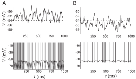
Figure 4: The regular (A) and irregular (B) firing modes of an integrate-and-fire model neuron. In the upper panels it is shown the membrane potential of the neuron when the spike generation mechanism is turned off (the dashed line is the spike threshold), while in the lower panels the membrane potential of the same neuron when the spiking mechanism is active. (Source: Dayan & Abbott, 2001)

7 Neural networks

By using different experimental methods has been proved that different cerebral areas are specialized for single functions (Kandel et al., 1999; Nicholls et al., 1997), even if no single areas are entirely responsible for a complex mind faculty. Indeed each area performs only some basic operations. In particular, all the most complex faculties are due to series and parallel connections across many different cerebral areas (Nicholls et al., 1997). In summary, extensive synaptic connectivity is a hallmark of neural circuitry. For example, a pyramidal neuron in the mammalian neocortex receives about 10,000 synaptic inputs where 75% are excitatory synapses and 25% inhibitory (this numbers change across the different structures of the cortex) (Abeles, 1991; Braitenberg & Schüz, 1991). The merging of a so high number of synaptic inputs on a single-neuron of the cortex is indicative of how broad is the integration of the signal that happens at the single-neuron level and, more in general, of how complex is the computation underlying each recording site. Network models allow us to explore the computational potential of such connectivity, using both analysis and simulation.

Networks are used to study a broad spectrum of phenomena such as selective amplification of inputs, short-term memory, gain modulation, input selection, coding of sensory stimuli and so on. Neocortical circuits are the focus of our discussion. In the neocortex, neurons lie in six vertical layers highly coupled within cylindrical columns. Such columns have been suggested as basic functional units, and stereotypical patterns of connections (both within a column and between columns) are repeated across cortex. In particular, we can divide the observed interconnections within cortex in three main classes (Dayan & Abbott, 2001):

• feedforward connections, the input travels in a defined direction going from a given area (or layer) to another located in a following stage along the signal pathway

• top-down connections, the input travels in a defined direction going from a given area (or layer) to another located in an earlier stage along the signal pathway

• recurrent connections, the neurons are interconnected within a given area which is considered to be at the same stage along the processing pathway

There is another major distinction between neural networks: they can be firing-rate or spiking models. In the former case each neuron-like unit of the network has output consisting of firing rates rather than action potential. This simplification is very useful to allow analytical calculations of same aspects of network dynamics that could not be treated in the case of spiking neurons. When we are dealing with spiking neurons networks, it means that the neuron-like unit of the network implements a model of action potential generation, so the output is given by the membrane potential and the spike train of each neuron.

The last classification of neural networks models we introduce is based on the kinds of single neurons that compose the network. In particular, if all the neurons belong to the same population of excitatory either inhibitory neurons, then we have a one-population network, while, when both the populations are present, the network is a two-population network. Eventually, if all the neuron of a given population have identical free parameters, the network is homogeneous, while, if the single-neuron parameters can differ from neuron to neuron (at fixed population), the network is inhomogeneous.

In this work we will investigate neural dynamics by means of two-populations recurrent networks of LIF neurons (that is spiking neurons).

2 Information Theory

A major purpose of our investigation of network dynamics by means of models is to understand the way neuronal networks convey information about sensory stimuli. Indeed the information calculation allows as to answer the following important question: “How much does the neural response tell us about a stimulus?”; by answering this question we can also investigate which forms of neural response are optimal for conveying information about natural stimuli.

In order to quantify the information transmitted by neurons, we treat the brain as a communication channel and we assume that the coding and transmission processes are stochastic and noisy. More precisely, we compute the Shannon mutual information (Shannon, 1948) between two random variables (Panzeri et al., 2007; Quiroga & Panzeri, 2009; Shannon, 1948) to quantify and analyze the information about the external stimulus obtained from different neural codes (i.e., different neural responses, as done in our previous work Mazzoni et al. (2011)) and with different synaptic current models (see chapter 2).

1 Shannon information and neuroscience

We introduce now the general concept of mutual information (hereafter information) of two random variables and we make, for clarity, examples by referring to our (discretized) case. Each time we run a simulation of a network model, we are basically computing an output signal as a function of the (noisy) input we inject to the network during the time interval $T$. We call that input signal the stimulus, $S$. In order to compute the information (that is the information of two random variables, where one is the stimulus $S$ and the other is the answer $R$) we need to define the neural response, $R$, that is the variable (or the set of variables) we take as output of the model. Note that this is the most important choice we make when computing information because it defines the neural code used to convey information, reflecting our hypotheses about which are the most important aspects of neural activity. We just mentioned that the response $R$ can be given by one or more variables; more in general, it can be a scalar quantity or a vector (“response vector”) and the dimension of the response, $L$, is the dimension of the code.

For each presentation of the stimulus $s$ in the time interval $T$, the response $R$ will assume the value $r$, and the amplitude of $T$ determines the temporal precision of the code.

A crucial point in this computation relies on the fact that the coding is a stochastic and noisy process: the value of the response $r$ does not depend on the stimulus $s$ in a deterministic way. Indeed the response is a stochastic function of the input where the noise plays a crucial role. This reflects a basic neuronal feature: real neurons are “noisy”, that is they can produce different responses when presenting the same external stimulus. Two recordings (or simulations) where the stimulus $s$ is the same, which differ only for the stochastic (noisy) component are called “trials”. By means of information we want to investigate the relationship between the stimulus $S$ and the answer $R$ by quantifying which is the average reduction in the uncertainty of $S$ due to the observation of $R$ (decoding point of view) or, equivalently, which is the average reduction in the uncertainty of the response $R$ due to the presentation of the stimulus $S$ (encoding point of view).

Let’s assume the decoding point of view, and introduce the way to quantify the average level of uncertainty associated with the stimulus $S$. We define the probability that stimulus $s$ is presented as: $P(s)=N_{s}/N_{tot}$, where $N_{s}$ is the number of times the stimulus $s$ has been presented and $N_{tot}$ the total number of stimuli presented. We can now introduce the (Shannon’s) total stimulus entropy:

$$H(S)=-\underset{s}{\sum}P(s)\log_{2}P(s),$$ (15)

where, by convention, base 2 logarithms are used so that information can be compared easily with results for binary systems. To indicate that the base 2 logarithm is being used, information is reported in units of “bits”. This quantity is the average uncertainty about which stimulus $s$ is presented in a time interval $T$. Indeed if the stimuli $s$ are all equal, $H(S)=0$, while it reaches its maximum when all the presented stimuli are different and equally likely: $H(S)=-\log_{2}(1/N_{tot})$.

We define similarly the Shannon’s total entropy of the stimulus $S$ given the response $R$:

$$H(S|R)=-\sum_{r,s}P(r)P(s|r)\log_{2}P(s|r),$$ (16)

where $P(r)$ is the probability that response $r$ is observed and $P(s|r)$ is the conditional (prior) probability that the stimulus $s$ was presented when the response $r$ is observed. This quantity represents the average uncertainty about which stimulus $s$ was presented in a time interval $T$ where the response $r$ is known. We can now define the mutual information between the response and the stimulus as the average reduction in the uncertainty of $S$ due to the observation of $R$ (in a time interval $T$):

$$I(S;R) = H(S)-H(S|R)$$ (17)

$$= \sum_{s,r}P(r)P(s|r)\log_{2}\frac{P(s|r)}{P(s)}.$$

The total stimulus entropy $H(S)$ represents the maximum information theoretically available with the given distribution of stimuli (irrespective of the code chosen). On the other hand, if $S$ and $R$ are independent, there is no reduction of the stimulus uncertainty due to the knowledge of the response, $H(S|R)=H(S)$, and the information is 0. The information, like entropy, is measured in bits; each bit of information corresponds to an average reduction of the uncertainty about the presented stimulus of a factor 2 as a consequence of the observation of a response $r$ in the time interval $T$. Note that the information (measured in bits) is obtained from the observation of the neuronal response over a time interval $T$, therefore it does depend on this value. In some cases it is useful to normalize the information by T to obtain units of bits/sec.

The Bayes theorem relates the prior probability $P(s|r)$ to the current probability $P(r|s)$ in the following way:

$$P(s|r)=\frac{P(r|s)P(s)}{P(r)}.$$ (18)

By using the Bayes theorem in the equation 17, we obtain:

$$I(S;R) = H(S)-H(S|R)$$ (19)

$$= \sum_{s,r}P(s,r)\log_{2}\frac{P(s,r)}{P(s)P(r)}$$

$$= \sum_{s,r}P(s)P(r|s)\log_{2}\frac{P(r|s)}{P(r)}$$

$$= H(R)-H(R|S)=I(R;S),$$

where $P(s,r)=P(s)P(s|r)=P(r)P(r|s)$ is the joint probability of stimulus $s$ appearing ans response $r$ being evoked.

From equation 5 we conclude that information is symmetric with respect to interchange of $S$ and $R$. This is the reason why the information is mutual: $S$ and $R$ can be inverted without affecting the information. In the end we demonstrated what we mentioned above: the average reduction in the uncertainty of $S$ due to the observation of $R$ is equivalent to the average reduction in the uncertainty of the response $R$ due to the presentation of the stimulus $S$.

This last point of view (encoding point of view, corresponding to the last row of equation 5) represents a different interpretation of information which is based on the fact that the more the response is variable, the higher is the theoretical capacity of a code to convey information. Indeed an higher level of variability in the response $R$ corresponds to an higher value of the total response entropy, $H(R)$, which represents the maximum information theoretically achievable with the given code (distribution of responses) (de Ruyter van Steveninck et al., 1997; Dayan & Abbott, 2001). The variability in the response as measured by the total response entropy includes both the variability due to the presentation of different stimuli and to the noise (which gives rise to different responses when the stimulus is fixed). The latter contribution is the entropy of the response $R$ given the stimulus $S$, $H(R|S)$, that is indeed called the noise entropy. Therefore $I(S;R)=H(R)-H(R|S)$ is the variability in the response only due to the presentation of different stimuli.

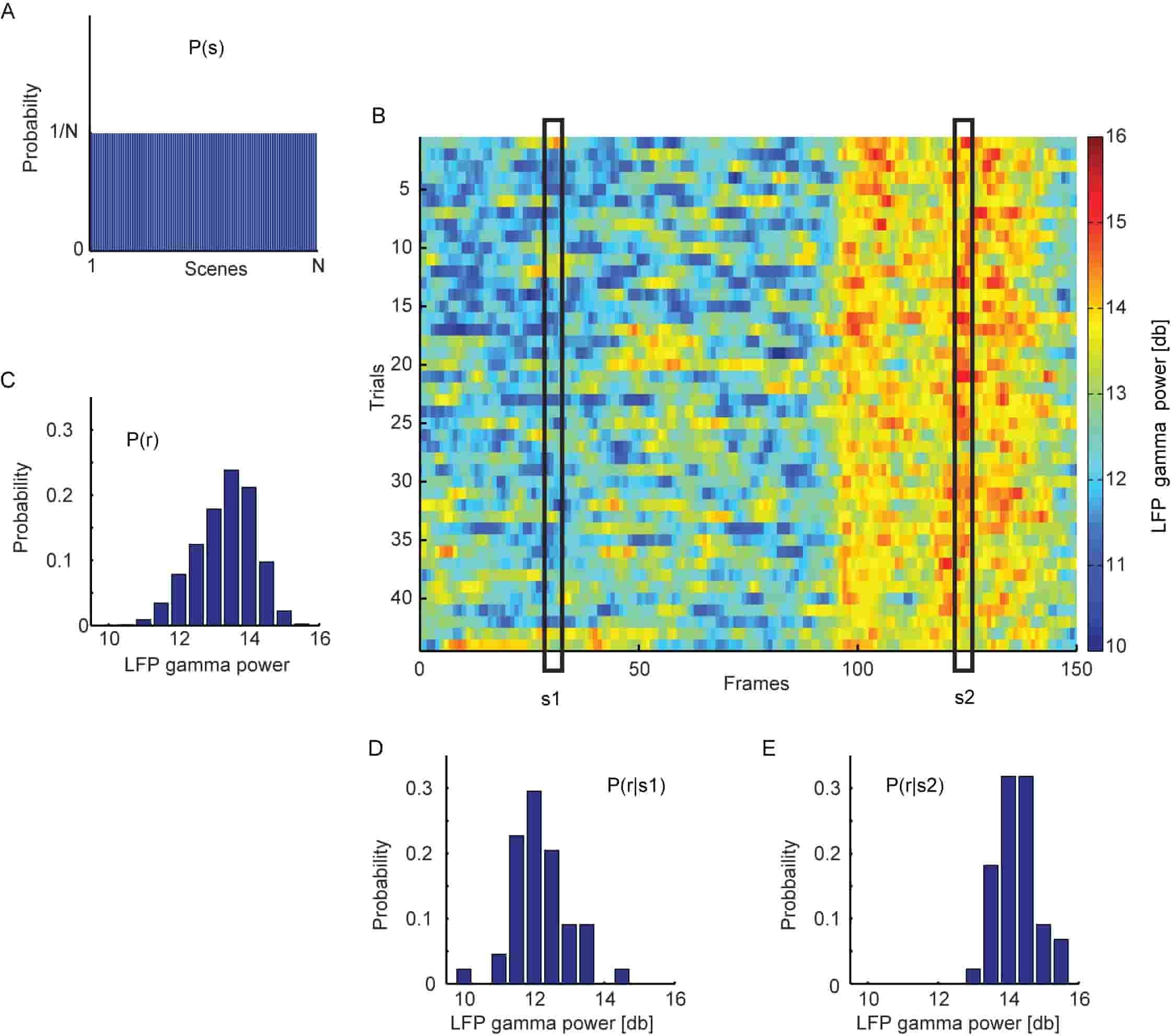
Figure 5: Schematic representation of the computation of the mutual information carried by LFP power about movie scenes of a complex visual stimulus. The figure illustrates the way to obtain the different probabilities needed to compute the information $I(S;R)$ (see equation ) in a specific case where the stimulus, $S$, is the Hollywood movie presented to a monkey and the response, $R$, is the LFP power in the gamma band. (A) First the entire movie presentation time is portioned into non-overlapping window, each considered a different stimulus $s$ (a “scene”). The set of the stimuli is the set of the different scenes, each of which is presented once every trial, therefore the probability of each scene, $P(s)$, is the inverse of the number $N$ of the scenes presented and it is constant. (B) The color plot shows the single-trial LFP gamma power (in this example, in the [72–76 Hz] frequency range) across all trials and movie scenes. From these data it is possible to compute the (C) probability distribution $P(r)$ of the LFP gamma power across all trials and scenes and (D, E) the probability distribution $P(r|s)$ of the LFP gamma power across trials given the presented scenes $s1$ and $s2$ respectively. The differences between the two distributions and the distribution $P(r)$ suggest that the LFP gamma power carried information about which scene is presented. By computing $P(r|s)$ for all scenes and inserting it in equation the actual value of the mutual information is obtained. (Adapted from Mazzoni et al. (2011))

In figure 5 is showed a schematic representation of the computation of the mutual information in an example case where the stimulus is given by a movie presented to a monkey and the response is the power of LFP oscillations in a given frequency band.

We can extend the information computation to the case where we want to quantify how much information is conveyed by the simultaneous observation of two distinct responses $R_{1}$ and $R_{2}$ (for example the power spectral density of two frequencies of the LFP). In this case the mutual information is:

$$I(S;R_{1},R_{2})=\sum_{s,r}P(s)P(r_{1},r_{2}|s)\log_{2}\frac{P(r_{1},r_{2}|s)}{P(r_{1},r_{2})}$$ (20)

If the two responses $R_{1}$ and $R_{2}$ were tuned to independent stimulus features, and they do not share any source of noise, then we would expect that $I(S;R_{1},R_{2})=I(S;R_{1})+I(S;R_{2})$, which means that the two responses convey completely independent information about the same stimulus. Therefore to quantify how independent are the contributions to information given by the two responses we introduce the following information redundancy (Gieselmann & Thiele, 2008; Logothetis, 2002; Logothetis et al., 2007):

$$Red(R_{1},R_{2})=I(S;R_{1})+I(S;R_{2})-I(S;R_{1},R_{2}).$$ (21)

Redundancy is never negative, when it is zero, the two responses convey completely independent information about the stimulus, otherwise (at least part of) the information carried by $R_{1}$ and $R_{2}$ is redundant (is the same).

We conclude this section by pointing out some important features that underlain information computation when evaluating the relationship between the stimulus and the neural activity evoked:

• it is simple and allows a easy comparison between data obtained from experiments and from models (Mazzoni et al., 2011)

• there are no assumptions about which features of the stimulus shape the neuronal response and in this way no one is missed (de Ruyter van Steveninck et al., 1997)

• what matters when computing information is the probability to observe the answer $r$ when presenting the stimulus $s$, therefore the units of the answer do not matter. This allows to build codes where the answer $R$ combines different measurements of the neural activity (for example the spiking activity and the LFP) observed in time intervals of amplitude $T$. In the latter case we speak of “nested” codes (Kayser et al., 2009), to distinguish them from the case where the response is given by a single variable (like the firing rate or the spike time). Furthermore the response $r$ (defined in the time interval $T$) can include variables measured on different temporal scales, $\varDelta t\leq T$. For example, it can be represented by the precise timing of individual spikes on the scale ($\varDelta t$) of milliseconds and by the phase of the slow oscillations of the concomitant LFP on the scale ($T$) of hundreds of milliseconds. In these cases we call the code a “multiplexed” code (Panzeri et al., 2010).

3 Neural encoding and decoding

A fundamental issue in neuroscience is the investigation of the link between stimulus and response. In section 1, we saw that by means of the mutual information we can characterize “how much” the neural response tells us about the presented stimulus. An alternative and complementary approach to the same matter focus on the question: “What does the response of a neuron tell us about a stimulus?” Neural encoding and decoding face precisely this question.

We already showed that when computing information the stimulus and the response can be interchanged without affecting the result. Thus, from a mathematical point of view, there is not an a priori distinction between the stimulus and the answer… it is just matter of choice. On the other hand, when you are doing an experiment it is always the case that it is clear which is the stimulus (if there is) you are presenting/injecting and which is the response you are recording. This is the reason why there are the two distinct names: neural encoding and decoding. Neural encoding refers to the map from stimulus to response, while neural decoding refers to the reverse map.

1 Spike trains and firing rates

In real neurons, action potentials can vary somewhat in duration, amplitude, and shape. However, when dealing with neural coding, action potentials are typically treated as identical stereotyped events and what matters is only the spike timing. Thus, we ignore the duration of an action potential (about 1 ms), and characterize the firing activity of a neuron by means of a list of the times when spikes occurred: for $n$ spikes, we denoted these times by $t_{i}$ with $i=1,2,...,n$. From the mathematical point of view, we assume the spike sequence can be represented as a sum of Dirac $\delta$ functions:

$$\rho(t)=\stackrel{{\scriptstyle[}}{{i}}=1]{n}{\sum}\delta(t-t_{i}).$$ (22)

$\rho(t)$ is the spike train (or neural response function; it represents the spiking times). Because of the trial-to-trial variability of the neural response, $\rho(t)$ is typically treated statistically or probabilistically (see section 1). Thus we use angle brackets, $\langle\rangle$, to denote average over trials at fixed stimulus and we introduce the trial-averaged spike train,$\langle\rho(\tau)\rangle.$ Then the “average firing rate” over a time window $T$ is given by:

$$\langle r\rangle=\frac{1}{T}\int_{0}^{T}d\tau\langle\rho(\tau)\rangle,$$ (23)

while the firing (or spiking) rate, $r(t)$, has the following expression:

$$r(t)=\frac{1}{\varDelta t}\int_{t}^{t+\varDelta t}d\tau\langle\rho(\tau)\rangle.$$ (24)

This is the “firing rate” computed on time windows of amplitude $\varDelta t$. Formally the dependence on $\varDelta t$ can be removed by taking the limit $\varDelta t\rightarrow 0$ on the right hand side of the equation (that is $r(t)=\langle\rho(t)\rangle$). Actually the firing rate, $r(t)$, being a probability density, cannot be determined exactly from the limited amounts of data available from a finite number of trials. Therefore we need to approximate the true firing rate from a spike sequence. There are several procedures to do it and some of them are illustrated in figure 6. A very common way consists in making the convolution of the available spike train, $\rho(t)$, (or the PSTH, see figure 6) with a window function (also called the filter kernel), $w(t)$, in order to obtain a more smoothed signal (and avoid jagged curve, like the ones showed in figure 6B,C):

$$r(t)=\int_{-\infty}^{+\infty}d\tau w(\tau)\rho(t-\tau),$$ (25)

where $w(\tau)$ goes to 0 outside a region near $\tau=0$ and has time integral equal to 1 (in order to not affect units of the firing rate). The filter kernel specifies how the spike train evaluated at time $t-\tau$ contributes to the firing rate approximated at time $t$. Therefore, if we want the approximated firing rate in $t$ depends only on the spikes occurred before $t$, the window function must be 0 when its argument is negative. Such a kernel is termed causal.

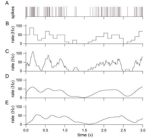
Figure 6: Different procedures to approximate the firing rate. (A) Sampled spike train of a neuron, $\rho(t)$. (B) This is a discrete time approximation of the firing rate called Post Stimulus Time Histogram (PSTH) obtained by dividing time into bins of fixed amplitude (here $\varDelta t=100$ ms) and counting the number of spikes within each bin. (C) Approximate firing rate obtained by the discrete version of equation 24 with $\varDelta t=100$ ms. (D) Approximate firing rate computed using equation 25 with $w(t)$ is a Gaussian window function with $\sigma_{t}=100$ ms. (E) Approximate firing rate computed using equation 25 with a causal window function ($\alpha$ function). (Source: Dayan & Abbott, 2001)

2 Spike-triggered average

A simple and effective way to perform neural encoding (that is to characterize the average neural response to a given stimulus) is to count the (trial-averaged) number of action potential fired during the presentation of different stimuli. By plotting this number as a function of the parameters $s$ chosen to characterize the stimuli, we obtain the response tuning curve. The neural response to an external stimulus is mediated by the interaction between the stimulus and the sensory surface (e.g. in case of visual stimuli between the presented image and the retina). The portion of the sensory surface (and, by extension, of the external stimulus) responsible for the modulation of the firing activity of a given neuron is called the receptive field of the neuron.

Response tuning curve characterizes the average neural response to a given stimulus. The complementary procedure, when performing neural decoding, consists in computing the average stimulus that elicited a given response. If the response is the spiking activity, this means to compute the spike-triggered average (STA). Indeed, the spike-triggered average is the average value of the stimulus at a time interval $\tau$ from the occurrence of a spike. We describe the stimulus with a parameter, $s(t)$, that varies over time, and define the STA as:

$$C(\tau)=\frac{1}{\langle n\rangle}\int_{0}^{T}dt\langle\rho(t)\rangle s(t-\tau)=\frac{1}{\langle n\rangle}\int_{0}^{T}dt\>r(t)s(t-\tau),$$ (26)

where $\langle n\rangle$ is the average number of spikes in each trial, which is assumed to be constant over trials. Although the range of $\tau$ values in equation 26 extends over the entire trial length time, the response is typically affected only by the stimulus in a window a few hundred milliseconds wide immediately preceding and following a spike. To understand the reason of this behavior, let’s introduce the cross-correlation between the firing rate and the stimulus:

$$Q_{rs}(\tau) = \frac{1}{T}\int_{0}^{T}dt\>r^{\ast}(t)s(t+\tau)$$

$$= \frac{1}{T}\int_{0}^{T}dt\>r(t)s(t+\tau).$$

By substituting equation 2 into equation 26, we obtain that

$$C(\tau)=\frac{T}{\langle n\rangle}Q_{rs}(-\tau)=\frac{Q_{rs}(-\tau)}{\langle r\rangle}.$$ (28)

Now it is clear than the STA will approach to zero for positive $\tau$ values larger than the correlation time between the stimulus and the response (that is usually in the order of hundred of milliseconds or smaller). Furthermore the response of a neuron cannot depend on future stimuli, thus, unless the stimulus has temporal autocorrelation, we expect for $C(\tau)$ to be zero for $\tau<0$.

Because of the minus sign of the argument in the right hand side of equation 28, the spike-triggered average is also called “reverse correlation function”.

3 Reverse correlation and Wiener kernels

When investigating the relationships between network oscillations such as LFPs and EEGs and single-neuron activity, we cannot use (a priori) the categories of stimulus and answer. Indeed we do not know if there are (and in which directions) causal relationships between the two signals. In this respect, neither we can talk of neural encoding nor decoding. Our purpose is to estimate the time course of the local field potentials from the spiking activity of a neuron and vice versa. We also want to test how robust and general can be this estimation.

If we have a nonlinear system, where the input $x(t)$ and the output $y(t)$ are functions of the time related by some functional transformation $y(t)=F[x(t)]$, methods developed by Volterra (Volterra, 2005) and Wiener (Wiener, 1966), provide a power series expansion of the output function:

$$y(t) = h_{0}+\int_{-\infty}^{+\infty}d\tau\>h_{1}(\tau)x(t-\tau)$$

$$+\int_{-\infty}^{+\infty}d\tau_{1}\int_{-\infty}^{+\infty}d\tau_{2}\>h_{2}(\tau_{1},\tau_{2})x(t-\tau_{1})x(t-\tau_{2})$$

$$+\int_{-\infty}^{+\infty}d\tau_{1}\int_{-\infty}^{+\infty}d\tau_{2}\int_{-\infty}^{+\infty}d\tau_{3}\>h_{3}(\tau_{1},\tau_{2},\tau_{3})x(t-\tau_{1})x(t-\tau_{2})x(t-\tau_{3})+\ldots$$

Under certain conditions, the proper choice of the (Volterra) kernels, $h_{n}$, will provide a complete description of any transformation $x(t)\rightarrow y(t)$ (Volterra, 2005). Note that, in general, this is not a causal reconstruction of the output signal $y$, indeed the integrals can range over negative values of the time variable $\tau$, which means that the value of the input $x$ at time instants later than $t^{\ast}$ can affect the value of $y(t^{\ast})$. The series was rearranged by Wiener to make the terms easier. In particular, Wiener reformulated Volterra’s expansion by making the successive terms independent, which means that we can compute the terms individually. In this formulation, the filter kernels are called Wiener kernels.

Since we are interested in building a linear model of the relationships between single-neuron activity and network oscillations, let’s focus on the first (i.e., linear) Wiener kernel $h_{1}$. To have a clear intuition of what we are doing, remember that the simplest way to construct an estimate of a time varying signal $y$ starting from $x$, $y_{est}$, is to assume that at any given time, $t^{\ast}$, $y_{est}(t^{\ast})$ can be expressed as a weighted sum of the values taken by $x$. Let’s assume that the weights are constant in time (i.e., they are not a function of the time instant $t^{\ast}$: the estimation is time invariant), therefore we write the estimated signal as the convolution between a kernel $h_{x2y}$ and the input signal (plus a constant $y_{0}$),

$$y_{\mathrm{est}}(t) = y_{0}+\int_{0}^{T}d\tau\>h_{x2y}(t-\tau)x(\tau),$$ (30)

$$= y_{0}+\int_{t-T}^{t}d\tau\>h_{x2y}(\tau)x(t-\tau).$$ (31)

The Wiener filter $h_{x2y}$ gives the weights of the sum (that is the integral on time): it determines how strongly, and with what sign, the value of the input $x$ in $(t-\tau)$ contribute to the value of the output in $t$. Since we are dealing with real signals, the integral does not range from minus to plus infinity (as in equation 3) but it is restricted over the time interval where the signals are defined (from 0 to $T$, the length of the trial). Note that in equation 30 (and hereafter) the signal $x(t)$ is defined with its mean value subtracted out (that is $\int_{-\infty}^{+\infty}dt\>x(t)=0$), thus the constant term $y_{0}$ is the mean value of $y_{est}$ and compensates for the mean subtraction done on $x$ and it also accounts for any background output activity we could have when $x=0$.

The filter $h_{x2y}$is chosen to minimize the mean (over the duration of the trial, $T$) squared distance (MSD) between the original signal, $y$, and the estimated one, $y_{est}$:

$$\mathrm{MSD}(y,y_{\mathrm{est}})=\frac{1}{T}\int_{0}^{T}dt[y(t)-y_{\mathrm{est}}(t)]^{2}.$$ (32)

By minimizing this expression it is possible to obtain an explicit formula for the Fourier transform of the Wiener optimal kernel$:$

$$\tilde{h}_{x2y}(\omega)=\frac{\tilde{Q}_{xy}(\omega)}{\tilde{Q}_{xx}(\omega)}=\frac{\tilde{Q}_{yx}(-\omega)}{\tilde{Q}_{xx}(\omega)}$$ (33)

thus

$$h_{x2y}(t)=\frac{1}{2\pi}\int_{-\infty}^{+\infty}d\omega\>\frac{\tilde{Q}_{xy}(\omega)}{\tilde{Q}_{xx}(\omega)}e^{-i\omega t},$$ (34)

where the $\tilde{f}$ indicates the Fourier transform of $f$. $Q_{xy}(\omega)$ is the cross-correlation between x and y (see equation 2) and $Q_{xx}(\omega)$ is the autocorrelation. The Wiener-Khinchin theorem assures that if $x$ and $y$ are wide-sense stationary random processes, $\tilde{Q}_{xy}$ can be computed as the cross power spectral density of $x$ and $y$, $S_{xy}(\omega)$, and $\tilde{Q}_{xx}$ as the power spectral density of $x$, $S_{xx}(\omega)$. Since the mean value of $x$ is zero, the convolution theorem (i.e., $\widetilde{f\ast g}=k\,\tilde{f}\,\tilde{g}$) implies that the mean value of the kernel, $h_{x2y}$, is zero.
Note that the Wiener kernel can be seen also as the transfer function of the linear time-invariant system made by the input $x$ and the output $y$.

To have a more clear idea of what the kernel represents suppose that the input $x(t)$ is an uncorrelated signal (i.e., its autocorrelation is a delta function: $Q_{xx}(\tau)=k\delta(\tau)$), as in the case of white noise, and the output is a firing rate $y=r(t)$. Thus, from equation 33, we obtain:

$$h_{x2r}(\tau)=\frac{Q_{rx}(-\tau)}{k}=\frac{\langle r\rangle C(\tau)}{k},$$ (35)

where $C(\tau)$ is the STA and the last equality follows from equation 28. Therefore in case of white-noise input and spike train output, the first Wiener kernel is proportional to the spike-triggered average. On the other hand, if the input is an uncorrelated firing rate, $r(t)$, (which tends to happen at low rates), $Q_{rr}(\tau)=\langle r\rangle\delta(t)$, the equation for the Wiener kernel becomes:

$$h_{x2r}(\tau)=\frac{Q_{ry}(\tau)}{\langle r\rangle}=C(-\tau).$$ (36)

We conclude this section by noting that comparing equations 36 and 33 we can have a better insight on the difference between the STA and the Wiener kernel when performing a decoding task. In particular, the numerator in equation 33 reproduces the STA in equation 36, thus the role of the denominator in the expression of the Wiener kernel is to correct for the autocorrelation in the response spike train. Indeed such autocorrelation introduce a bias in the decoding, which is removed by using the Wiener kernel. Note that, when the input is a firing rate, the convolution in equation 30 translates into a simple rule: every time a spike appears, we replace it with the kernel.

Causality in the estimation

The linear estimation performed by using equation 30 is not causal in general, indeed the argument of the kernel can range over negative values. The simplest way to force the estimation of $y$ to be causal is to set the kernel equal to 0 for negative values (i.e., $h_{x2y}(t)=0$ for $t<0$), or, equivalently, to restrict the interval of integration in equation 30:

$$y_{\mathrm{est}}^{\mathrm{causal}}(t)=y_{0}+\int_{0}^{t}d\tau\>h_{x2y}(t-\tau)x(\tau).$$ (37)

A complementary procedure useful to implement causality is given by the introduction of a delay in the filter (Dayan & Abbott, 2001). In equation 30 we attempt to estimate the signal $y$ in $t$ by using the values of $x$ over the entire trial length, while in equation 37 we use only the value of $x$ prior to the time $t$. We already mentioned that, when we are dealing with decoding tasks, the signal $y(t)$ we want to estimate is the stimulus and $x(t)$ is the elicited response (e.g. spike-train decoding: we attempt to construct an estimation of the stimulus from the evoked spikes). The stimulus required a finite amount of time $\tau_{0}$ to affect the response, thus, to make the decoding task easier we can introduce a prediction delay $\tau_{0}$ and estimate the stimulus $y$ at time $(t-\tau_{0})$ from the values of the response $x$ up to time $t$:

$$y_{\mathrm{est}}(t-\tau_{0})=y_{0}+\int_{0}^{t}d\tau\>h_{x2y}(t-\tau)x(\tau).$$ (38)

The delay $\tau_{0}$ results in the Wiener kernel expression in the following way:

$$\tilde{h}_{x2y}(\omega)=\frac{\tilde{Q}_{xy}(\omega)}{\tilde{Q}_{xx}(\omega)}e^{i\omega\tau_{0}},$$ (39)

and equation 36 becomes:

$$h_{x2y}(\tau)=\frac{Q_{ry}(\tau-\tau_{0})}{\langle r\rangle}=C(\tau_{0}-\tau).$$ (40)

Note that, if there is not stimulus autocorrelation, $C(\tau)=0$ for $\tau<0$ (i.e., the filter is zero for $\tau>0$). On the other hand, the causality requires the filter to be zero for $\tau<0$. Therefore, from equation 40, it is clear the need for either stimulus autocorrelation or a nonzero prediction delay $\tau_{0}$ when $x$ is the stimulus and $y$ the response.

Chapter 2 How synaptic currents shape network dynamics

In this chapter we investigate in a modelling framework some aspects of the relationship between dynamics at the single-neuron and at the network level. More precisely, we focus on how different features of the synaptic input affect network dynamics as measured by LFPs and average properties across neurons.
We already mentioned that models of networks of Leaky Integrate-and-Fire (LIF) neurons are a widely used tool for theoretical investigations of brain functions. These models have been used both with current- and conductance-based synapses (see section 6). However, the differences in the dynamics expressed by these two approaches have been so far mainly studied at the single-neuron level. To investigate how these synaptic models affect network activity, we compared the single-neuron and neural population dynamics of conductance-based networks (COBNs) and current-based networks (CUBNs) of LIF neurons. These networks were endowed with sparse excitatory and inhibitory recurrent connections, and were tested in conditions including both low- and high-conductance states. We developed a novel procedure to obtain comparable networks by properly tuning the synaptic parameters not shared by the models. The so defined comparable networks displayed an excellent and robust match of first order statistics (average single-neuron firing rates and average frequency spectrum of network activity). However, these comparable networks showed profound differences in the second order statistics of neural population interactions and in the modulation of these properties by external inputs. The correlation between inhibitory and excitatory synaptic currents and the cross-neuron correlation between synaptic inputs, membrane potentials and spike trains were stronger and more stimulus-modulated in the COBN. Because of these properties, the spike train correlation carried more information about the strength of the input in the COBN, although the firing rates were equally informative in both network models. Moreover, the network activity of COBN showed stronger synchronization in the gamma band, and spectral information about the input higher and spread over a broader range of frequencies. These results suggest that the second order statistics of network dynamics depend strongly on the choice of the synaptic model.

1 Introduction

Networks of Leaky Integrate-and-Fire (LIF) neurons are a key tool for the theoretical investigation of the dynamics of neural circuits. Models of LIF networks express a wide range of dynamical behaviors that resemble several of the dynamical states observed in cortical recordings (see Brunel (2013) for a recent review). An advantage of LIF networks over network models that summarize neural population dynamics with only the density of population activity, such as neural mass models (Deco et al., 2008), is that LIF networks include the dynamics of individual neurons. This allows to investigate at the same time the single-neuron and the network level, and, for example, LIF networks can be used to investigate phenomena, such as the relationships among spikes of different neurons, that are not directly accessible to simplified mass models of network dynamics.

A basic choice when designing a LIF network is whether the synaptic model is voltage-dependent (conductance-based model) or voltage-independent (current-based model). In the former case the synaptic current depends on the driving force, while this does not happen in the current-based model(see section 6). Current-based LIF models are popular because of their relative simplicity (see e.g. Brunel (2013)) and they have the key advantage of facilitating the derivation of analytical closed-form solutions. Thus current-based synapses are convenient for developing mean field models (Grabska-Barwińska & Latham, 2014), event based models (Touboul & Faugeras, 2011), or firing rate models (Helias et al., 2010; Ostojic & Brunel, 2011; Schaffer et al., 2013), as well as in studies examining the stability of neural states (Babadi & Abbott, 2010; Mongillo et al., 2012). Moreover, current-based models are often adopted, because of their simplicity, to investigate numerically network-scale phenomena (Memmesheimer, 2010; Renart & van Rossum, 2012; Gutig et al., 2013; Lim & Goldman, 2013; Zhang et al., 2014). On the other hand, conductance-based models are also widely used because they are more biophysically grounded (Kuhn et al., 2004; Meffin et al., 2004). In particular, only conductance-based neurons can reproduce the fact that when the synaptic input is intense, cortical neurons display a three- to fivefold decrease in membrane input resistance (thus they enter a high-conductance state), as observed in intracellular recordings in vivo (Destexhe et al., 2003). However, an added complication of conductance-based models is that their differential equations can only be evaluated numerically or approximated analytically (Rudolph-Lilith et al., 2012) rather than being fully analytically treatable.

Despite the widespread use of both types of models, the differences in the network dynamics that they generate has not been yet fully understood. Previous studies comparing conductance- and current-based LIF models focused mostly on the individual neuron dynamics (Kuhn et al., 2004; Meffin et al., 2004; Richardson, 2004). Here we extended these previous works by investigating the network level consequences of the synaptic model choice. In particular, we investigated which aspects of network dynamics are independent of the choice of the specific synaptic model, and which are not. Understanding this point is crucial for fully evaluating the costs and implications of adopting a specific synaptic model.

We compared the dynamics of two sparse recurrent excitatory-inhibitory LIF networks, a conductance-based network (COBN) with conductance-based synapses, and a current-based network (CUBN) with current-based synapses. To properly compare the two networks, we set to equal values all the common parameters (including the connectivity matrix). Building on previous works (La Camera et al., 2004; Meffin et al., 2004), we devised a novel algorithm to obtain two comparable networks by properly tuning the synaptic conductance values of the COBN given the set of values of synaptic efficacies of the CUBN. Since the differences between the dynamics of the two synaptic models depend on the fluctuations of the driving force (i.e., of the membrane potential), they should be close to zero when the synaptic activity is low. Thus, when decreasing the background synaptic activity, the Post-Synaptic Currents (PSCs) of the two models should become more and more similar. Consequently, our procedure calibrated the conductances so that PSCs became exactly equal in the limit of zero synaptic input (see section 6). Then we investigated whether this procedure could generate COBNs and CUBNs with matching average single-neuron stationary firing rates under a reasonably wide range of parameters and network stimulation conditions. We then studied how comparable conductance- and current- based networks differed in more complex characterizations of population dynamics, such as the cross-neuron correlations of membrane potential (MP), input current and spike train, as well as the spectrum of network fluctuations. The latter was investigated not only for total average firing rates, but also for the simulated Local Field Potential (LFP) computed from the massed synaptic activity of the networks (Mazzoni et al., 2008). To study the spectrum of network fluctuations it is useful to use a LFP model (rather than a massed spike rate) mainly because cortical rhythms are more easily measured in experiments by recording LFPs rather than the spike rate (Buzsaki et al., 2012; Einevoll et al., 2013); therefore this quantification makes the models more directly comparable to experimental observations. We then quantified how the external inputs modulate the firing rate, the LFP spectrum and the spike train correlation by using information theory (Quiroga & Panzeri, 2009; Crumiller et al., 2011). Finally, we discuss the similarities and differences of COBN and CUBN against recent experimental observations of dynamics of cortical network correlations (Lampl et al., 1999; Kohn & Smith, 2005; De La Rocha et al., 2007; Okun & Lampl, 2008; Ecker et al., 2010; Renart et al., 2010).

2 Methods

1 Network structure and external inputs

We considered two networks of LIF neurons with identical architecture and injected with identical external inputs. The only difference between the two networks was in the synaptic model: one was composed by neurons with conductance-based synapses and the other by neurons with current-based synapses (see section 6). The network structure we adopt was already used in other works such as (Brunel & Wang, 2003; Mazzoni et al., 2008, 2011). Each network was composed of 5000 neurons. Eighty percent of the neurons were excitatory, that is their projections onto other neurons formed AMPA-like excitatory synapses, while the remaining 20% were inhibitory, that is their projections formed (A-type) GABA-like inhibitory synapses. The 4:1 ratio is compatible with anatomical observations (Braitenberg & Schüz, 1991). The network had random connectivity with a probability of directed connection between each pair of neurons of 0.2 (Sjostrom et al., 2001; Holmgren et al., 2003), thus any neuron in the network received on average 200 synaptic contacts from inhibitory neurons and 800 from excitatory neurons (see figure 1). Both populations received a noisy excitatory external input taken to represent the activity from thalamocortical afferents, with inhibitory neurons receiving stronger inputs than excitatory neurons. This simulated external input was implemented as a series of spike times that activated excitatory synapses with the same kinetics as recurrent AMPA synapses, but different strengths

Figure 1: Network structure. The network is composed of 1000 inhibitory (blue) and 4000 excitatory LIF neurons (red). Connectivity is random, each directed pair of neurons is connected with a probability of 0.2. The size of the arrows represents schematically the different synaptic strengths. In addition to recurrent interactions both populations receive an external excitatory input. Adapted from (Mazzoni et al., 2008).

The input spike trains activating the model thalamocortical synapses were generated by a Poisson process, with a time varying rate, $\nu_{ext}(t)$, identical for all neurons. Note that this implied that the variance of the inputs across neurons increased with the input rate. $\nu_{ext}(t)$ was given by the positive part of the superposition of a “signal”, $\nu_{signal}(t)$, and a “noise” component , $n(t)$:

$$\nu_{ext}(t)=[\nu_{signal}(t)+n(t)]_{+}$$ (1)

The separation of signal and noise in the input spike rate was to reproduce the classical experimental design in which a given sensory stimulus is presented many times, with each presentation (or “trial”) eliciting different responses due to variations in intrinsic network dynamics from presentation to presentation. We achieved this by identifying the external stimulus with the signal term, $\nu_{signal}(t)$, (which was thus exactly the same across all trials of the same stimulus) and by using a noise term, $n(t)$, generated (as explained below) independently in each trial.

In this study we used three kinds of external signals.
For the majority of the simulations we used constant stimuli, $\nu_{signal}(t)=\nu_{0}$, (with $\nu_{0}$ ranging from 1.5 to 6 spikes/ms).
In a second set of simulations we used periodic stimuli made by superimposing a constant baseline term to a sinusoid: $\nu_{signal}(t)=A\sin(2\pi ft)+\nu_{0}$, where A = 0.6 spikes/ms; $f$ ranged from 2 to 16 Hz in figure 17 and from 2 to 150 Hz in figure 18 and $\nu_{0}$ was set to 1.5 (respectively 5) spikes/ms when studying the low- (respectively high-) conductance state.
We also used a time varying signal, called “naturalistic”, that reproduced the time course of Multi Unit Activity recorded from the LGN of an anesthetized macaque during binocular presentation of commercially available color movies(Belitski et al., 2008). More precisely, the MUA was measured as the absolute value of the high pass filtered (400–3000 Hz) extracellular signal recorded from an electrode placed in the LGN while the monkey was presented binocularly a color movie (we refer to Rasch et al., 2008 for full details on experimental methods). The MUA measured in this way is thought to represent a weighted average of the extracellular spikes of all neurons within a sphere of <140–300 mm around the tip of the electrode (Logothetis, 2003), and thus gives a good idea of the spike rate fluctuations of a patch of geniculate input to cortex during viewing of natural stimuli. We took 40 consecutive seconds of LGN MUA recordings during movie presentation, we divided it into 20 non-overlapping intervals of 2 seconds (ideally corresponding to different movie scenes) following the procedure used in (Belitski et al., 2008), and each interval was considered as a different visual stimulus. For the purposes of the present work, it is mainly useful to remind that the naturalistic input was a slow signal dominated by frequencies below 4 Hz.

The noise component of the stimuli, $n(t)$, was generated by an Ornstein-Uhlenbeck (OU) process with zero mean:

$$\tau_{n}\frac{dn(t)}{dt}=-n(t)+\sigma_{n}(\sqrt{2\tau_{n}})\eta(t),$$ (2)

where $\eta(t)$ is a Gaussian white noise. $\sigma_{n}^{2}$=0.16 spikes/ms is the (stationary, that is for $t\rightarrow\infty$) variance of the noise, while the stationary mean is 0. The time constant $\tau_{n}$ was set to 16 ms to have a cutoff frequency of 10 Hz. The OU process is a stationary, Gaussian, and Markovian process we chose for the two following reasons:

• the power spectrum, which is flat up to the cutoff frequency and then it decays as $f^{-2}$. Therefore it does not diverge and it has the highest power spectral density in the low frequencies, in agreement with what found in the background activity of the cortex (Mazzoni et al., 2011)

• It is a mean-reverting process. Indeed, the drift term is not constant (since it depends on the value assumed by the process) and it always tends to drift the variable towards its long-term mean (0 in our case).

Note that the trial-to-trial differences in the stochastic process generated by equation 2 were the first and largest source of trial-to-trial variability in the model (that is the variability at fixed stimulus, see section 1), the second and last being the fact that each neuron received an independent realization of the Poisson process with rate $\nu_{ext}(t)$.

In a specific set of control stimulations (figure 15), instead of the OU process described above, we used a Gaussian white noise with the same variance. Note that, for low frequencies, the power spectrum of the OU process was higher than the one of the white noise.

2 Single-neuron models

Both inhibitory and excitatory neurons were modeled as (LIF) neurons (see section 3). The leak membrane potential, $V_{leak}$, was set to -70 mV, the spike threshold, $V_{threshold}$, to -52 mV and the reset potential, $V_{reset}$, to -59 mV. The absolute refractory period was set to 2 ms for excitatory neurons and to 1 ms for inhibitory neurons (Brunel & Wang, 2003). Since we had no current injected into the neuron through an electrode, the equation for the sub-threshold dynamic of the MP of i-th neuron (see equation 12) took the form:

$$\tau_{m}\frac{dV^{i}(t)}{dt}=-V^{i}(t)+V_{leak}-\frac{I_{tot}^{i}(t)}{G_{leak}},$$ (3)

where $\tau_{m}$ is the membrane time constant (20 and 10 ms for excitatory and inhibitory neurons respectively), $G_{leak}$ is the leak membrane conductance (25 and 20 nS for excitatory and inhibitory neurons respectively) (Brunel & Wang, 2003) and $I_{tot}^{i}(t)$ is the total synaptic input current. The latter was given by the sum of all the synaptic inputs entering the i-th neuron:

$$I_{tot}^{i}(t)=\underset{N_{(i,AMPArec)}}{\sum}I_{AMPArec}^{i}(t)+\underset{N_{(i,GABA)}}{\sum}I_{GABA}^{i}(t)+I_{AMPAext}^{i}(t),$$ (4)

the value of $N_{(i,AMPArec)}$ (respectively $N_{(i,GABA)}$) being the set of excitatory (respectively inhibitory) neurons projecting into the i-th neuron, and $I_{AMPArec}^{i}(t)$, $I_{GABA}^{i}(t)$, $I_{AMPAext}^{i}(t)$ the different synaptic inputs entering the i-th neuron from: recurrent AMPA, GABA, and external AMPA synapses respectively.

The difference between current- and conductance-based synapses lied in the definition of these synaptic input currents and. Current-based synapses (see equations 10), $I^{CUBN}$, were modeled as follows:

$$I_{syn}^{CUBN}(t)=J_{syn}s_{syn}(t),$$ (5)

while conductance-based currents (see equation 8), $I^{COBN}$, as

$$I_{syn}^{COBN}(t)=G_{syn}s_{syn}(t)(V(t)-V_{syn}).$$ (6)

Both models had the same synaptic kinetics, that is the same functions $\varDelta s_{syn}(t)$ described the time course of the synaptic currents: every time a presynaptic spike occurred at time $t^{*}$, $s_{syn}(t)$ of the postsynaptic neuron was incremented by an amount described by a delayed difference of exponentials (see section 9) (Brunel & Wang, 2003):

$$\varDelta s_{syn}(t)=\frac{\tau_{m}}{\tau_{d}-\tau_{r}}\left[\exp\left(-\frac{t-\tau_{l}-t^{*}}{\tau_{d}}\right)-\exp\left(-\frac{t-\tau_{l}-t^{*}}{\tau_{r}}\right)\right],$$ (7)

where the latency $\tau_{l}$, the rise time $\tau_{r}$ and the decay time $\tau_{d}$ are shown in table 1.

Synaptic time constants (ms)	$\tau_{l}$	$\tau_{r}$	$\tau_{d}$
GABA	1	0.25	5
AMPA on inhibitory	1	0.2	1
AMPA on excitatory	1	0.4	2

Table 1: Synaptic time constants of both models.

CURRENT-BASED NETWORK
Synaptic efficacies, $J_{syn}$ (pA)
GABA on inhibitory	54
GABA on excitatory	42.5
AMPArecurrent on inhibitory	-14
AMPArecurrent on excitatory	-10.5
AMPAexternal on inhibitory	-19
AMPAexternal on excitatory	-13.75

Table 2: Synaptic efficacies of the current-based network.

The current-based synapses (see equation 10) were characterized by the synaptic efficacies $J_{syn}$ whose value are reported in table 2.On the other hand, the parameters shaping the conductance-based synapses (see equation 8) were the conductances, $G_{syn}$, and the reversal potential of the synapses, $V_{syn}$ (see table 3).

CONDUCTANCE-BASED NETWORK
Synaptic conductances (nS)
GABA on inhibitory	2.70
GABA on excitatory	2.01
AMPArecurrent on inhibitory	0.233
AMPArecurrent on excitatory	0.178
AMPAexternal on inhibitory	0.317
AMPAexternal on excitatory	0.234
Synaptic reversal potential (mV)
VGABA	-80
VAMPA	0

Table 3: Reference values of the synaptic parameters in the conductance-based model.

A useful parameter for conductance-based neuron analysis is the effective membrane time constant, $\tau_{eff}$ . Following a standard procedure, we computed the total effective membrane conductance for the i-th neuron as:

$$G_{tot}^{i}(t) =G_{leak}+\underset{N_{(i,AMPArec)}}{\sum}G_{AMPArec}s_{AMPArec}^{i}(t)+\underset{N_{(i,GABA)}}{\sum}G_{GABA}s_{GABA}^{i}(t)+$$

$$+G_{AMPAext}s_{AMPAext}^{i}(t)$$ (8)

and we rewrote equation 3 as follows:

$$\tau_{eff}^{i}(t)\frac{dV^{i}(t)}{dt}=-V^{i}(t)+\frac{G_{leak}V_{leak}+\underset{N(i,syn)}{\sum}G_{syn}s_{syn}^{i}(t)V_{syn}}{G_{tot}^{i}(t)},$$ (9)

where “syn” indicates: recurrent AMPA; GABA; external AMPA synapses and

$$\tau_{eff}^{i}(t)=\frac{\tau_{m}G_{leak}}{G_{tot}^{i}(t)}$$ (10)

is the effective membrane time constant. In particular, for the i-th neuron, the effective AMPA conductance is defined as $\sum_{N(i,AMPArec)}G_{AMPArec}s_{AMPArec}^{i}(t)+G_{AMPAext}s_{AMPAext}^{i}(t)$ and the effective GABA conductance as $\sum_{N(i,GABA)}G_{GABA}s_{GABA}^{i}(t)$ (see figure 5).

By looking at equation 9 we can have a new insight about the differences between the two synaptic models. Indeed, by comparing equation 9 (for the conductance-based neurons) with equation 14 (for the current-based model), we see that the former case differs from the latter essentially because of:

• the leak conductance $G_{leak}$ has been replaced by the total conductance $G_{tot}(t)\geq G_{leak}$, which is a function of the synaptic input to the neuron

• the membrane time constant $\tau_{m}$ has been replaced by the effective membrane time constant $\tau_{eff}(t)\leq\tau_{m}$, which is a function of the synaptic input to the neuron

As a consequence of the variability in the total conductance, $G_{tot}(t)$, the conductance-based neurons can switch from low- to high-conductance states (Destexhe et al., 2003) and vice versa. In particular, when the network activity increases, the neurons tend to move towards high-conductance states (see equation 8 and figure 5) and vice versa.

3 Numerical methods

Network simulations were done using a finite difference integration scheme based on the second-order Runge Kutta algorithm (Press et al., 1992), also known as the midpoint method, with time step $\varDelta t=0.05$ ms.

The noise, $n(t)$, was obtained from equation 2 by implementing an exact numerical simulation of the Ornstein-Uhlenbeck process(Gillespie, 1996). The temporal durations of the simulations varied from 4.5 s to 100.5 s, and they are specified in the figure captions. The regimes we investigated displayed average firing rates relatively low (0.4–13 Hz), thus, when computing the Inter-Spike Interval (ISI) and the pairwise spike train correlation, we used the longest simulation times (25.5 and 100.5 s) to obtain larger spike datasets. Since we studied stationary responses, the first 500 ms of the simulations were never included in any analysis. Analysis and simulations (the latter implemented using MEX file) were performed in Matlab. Both COBN and CUBN model source codes are available on the ModelDB sharing repository (http://senselab.med.yale.edu/ModelDB/ShowModel.asp?model=152539) with accession number 152539.

4 Spectral analysis

To compute the power spectrum we used the Fast Fourier Transform with the Welch method (pwelch function in Matlab), dividing the time window under investigation into eight subwindows with 50% overlap.

For the entrainment analysis showed in figure 18 in case of periodic inputs with frequency $f$, we bandpassed the LFP at the correspondent frequency f with a Kaiser filter with zero phase lag and 2 Hz bandwidth, very small passband ripple (0.05 dB) and high stopband attenuation (60 dB). We extracted then the instantaneous phase by means of the Hilbert transform of the signal. To quantify entrainment, we computed the phase coherence between the phase of the input signal and of the LFP at the corresponding frequency (Mormann et al., 2000). Phase coherence, which we computed using the CircStat toolbox (Berens, 2009), ranges from zero (no relationships between phases) to 1 (perfect phase locking between the two signals).

5 LFP as a measure of network-level dynamics

A very common way to track network dynamics, that are dynamics due to the overall integrative processes of networks of neurons, is by means of a signal called local field potential. LFPs are obtained by low pass filtering an extracellularly recorded signal (called extracellular field potentials), which represents the electric activity resulting from the neuronal processes of cells close to the recording site (Belitski et al., 2008). More precisely, from a theoretical point of view, the neurons are placed in an extracellular medium, which acts as a conductor, with a specific impedance ($\sim 200-400$ $\Omega/$cm depending on the neuronal site, Ranck (1963, 1966); Mitzdorf (1985); Nicholson & Freeman (1975)) higher than the one of a saline solution ($\sim 65$ $\Omega/$cm). This high impedance reflects the fact that ion moves around cells in a very limited space. In the extracellular recording, the inflow of positive ions (mainly Na⁺) inside a neuron, through an active regions of the membrane, corresponds to an inward current and the active region to a current sink. When the current flows inside the neurons, for the continuity equation of electric charge, the inactive regions of the membrane act as sources of charge for the active regions (that is, through the inactive regions outward currents will flow). The superposition of currents from all sinks and sources, due to the impedance of the extracellular medium, elicits an electric field called extracellular field potential (EFP). To obtain EFPs actually useful to investigate network dynamics (i.e., dynamics due to a population of neurons), the measurement is done with an electrode (or pipette) with a sufficiently low impedance and whose tip is not too close to the spike generation site of a single neuron (in order to to avoid that the action potentials from the single neuron prevail on the overall neuronal signal). The EFPs recorded in this way collect both integrative processes due to the dendritic/synaptic activity of neurons and spikes fired from a groups of neurons in the proximity of the recording site. These two different contributions can be reliably segregated by frequency band separation. In particular, with a low pass filter (with a cutoff around 200 Hz) we obtain LFP, while, a high pass filter cutoff of $\sim 500$ Hz is used in most recordings to obtain the multi-unit activity. From MUA we can then extract the spiking activity of small neural populations in a sphere of 100–300 $\mu$m radius, and, by performing a spike sorting, even of single (or few) neuron (i.e., the single-unit activity) (Logothetis, 2008).

The LFP reflects the perisynaptic activity of a neural population, which, to have an idea can be within 0.5-3 mm from the electrode tip. The size of the neural population is debated and depends on both the method used to measure it and on the kind of electrode used. In general, the slow oscillations seem to be correlated on higher distances than the fast oscillations, thus depending on neurons located in a larger area. LFP is thought to be given by a weighted sum of all the potential changes close to the electrode, which depends on the current flows in the extracellular space. The latter, in turn, are related to all the integrative subthreshold processes. These processes are not only due to synaptic activity (i.e., synaptic potentials), but also to other types of slow oscillations, like voltage-dependent membrane oscillations and spike afterpotentials, in areas such as the dendritic trees, not accessible by the spiking activity of few neurons. In conclusion, the LFP does not reflect the output of a cortical area, but rather the synaptic and dendritic processes and the local processing of the signal in the cortex (Logothetis, 2008).

Computation of simulated LFP

Figure 2: Schematic of the computation of the simulated LFP. The arrows indicate the direction of the flow of positive charges (i.e., cations) in the extracellular medium due to GABA (blue) and AMPA synaptic currents (red arrows). Left side: representation of a pyramidal neuron in an open field configuration with excitatory synapses (AMPA) on apical dendrites and inhibitory synapses (GABA) close to the soma. We computed the simulated LFP as the GABA currents minus the AMPA currents because the pyramidal neurons are usually in an open field configuration thus the dipoles generated by excitatory and inhibitory currents sum with the same sign along the dendrite (remember that, by convention, inhibitory currents are positive and excitatory currents negative, see equation 2). Right side: we summed only currents from synapses of pyramidal neurons because, due to their approximate open field arrangement, they contribute to LFP more than interneurons, which instead have a much less regular dendritic spatial organization. Therefore, the contribution from different interneurons tend to cancel out each other. (Source: (Mazzoni et al., 2011))

We computed from network activity the LFP by using a procedure that has been proposed in previous works (Mazzoni et al., 2008, 2010). More precisely, we computed the simulated LFP as the difference between the sum of the GABA currents and the sum of the AMPA currents (both external and recurrent) that enter all excitatory neurons. This quantity was then divided by the leak membrane conductance to obtain units of mV:

$$LFP=\frac{1}{G_{leak}}\left(\underset{i_{exc}}{\sum}I_{GABA}^{i}-\underset{i_{exc}}{\sum}I_{AMPAtot}^{i}\right).$$ (11)

As explained above in detail, LFPs are experimentally obtained by low-pass filtering the extracellularly recorded neural signal, and are thought to reflect to a first approximation the current flow due to synaptic activity around the tip of the recording electrode (Buzsaki et al., 2012). The simple recipe in equation 11, we used to model that current flow, was motivated by two well-known geometrical properties of cortical circuits (see figure 2). First, AMPA synapses tend to be apical, i.e., they contact the dendrites away from the soma, while GABA synapses tend to be peri-somatic, i.e., they contact the soma or the dendrites close to the soma. Because of this spatial arrangement, the sink and sources of the flow of cations resulting from the activation of both AMPA and GABA synapses will tend to produce in the extracellular field a dipole oriented from apical dendrites toward soma; hence we computed the LFP by subtracting the AMPA currents from the GABA currents (divided by the leak membrane conductance). Second, pyramidal neurons contribute more than interneurons to generation of LFPs in cortex because (i) they are bigger than interneurons eliciting stronger action potentials, furthermore (ii) their apical dendrites are organized in an approximate open field configuration (Johnston & Wu, 1995; Logothetis, 2003), thus the contribution of each pyramidal neuron sum up to each other (see figure 2). On the other hand, in the interneurons, due to their star-shaped dendrites and their geometrical disorder, contributions from each cell are smaller and tend to cancel out each other (Lorente de NO, 1947; Murakami & Okada, 2006; Linden et al., 2011). Therefore, we computed LFPs by considering only input currents to excitatory neurons (taken here to correspond to cortical pyramidal neurons).
Note that this model neglects all the contribution to the LFP not due to synaptic potentials and does not assume any dependencies of the contributions from different neurons on the topology of the network (indeed there are not weights in the summation in equation 11). Nevertheless, though simple, it proved to be an effective way to generate a realistic LFP signal that match many characteristics of LFPs in sensory cortex (Mazzoni et al., 2010, 2011, 2008).

6 Procedure to determine comparable current- and conductance-based models

As mentioned above all the parameters that were directly shared between the two models were set equal; also the connectivity matrix was the same in the CUBN and in the COBN. The starting point of our comparison was to completely define the CUBN, by specifying the synaptic efficacies, $J_{syn}$ (reported in table (2)), as well as the values of the common set of parameters. Then, we computed the synaptic parameters of the COBN that made it comparable to the given CUBN. To simplify the problem, we first set the reversal potentials of the COBN to biophysically plausible values: $V_{AMPA}$ = 0 mV and $V_{GABA}$ = −80 mV (as reference values, but we also tested other values, see figure 8C,D, 9D). The “free” parameters now left to set were only the COBN conductances ($G_{syn}$ in equation 6).

Figure 3: Procedure to set the synaptic conductances of the COBN. The flowchart illustrates the iterative algorithm we used to set the synaptic conductances, $G_{syn}$, such in a way to obtain a COBN comparable with the given CUBN. The two networks shared all the common parameters, so, once the CUBN was given, the synaptic conductances depended only on the synaptic reversal potentials of the COBN, $V_{syn}$.

The procedure used to obtain the conductance values leading to comparable COBN and CUBN is illustrated in figure 3 and described in the following. Consistent with the fact that the effective membrane time constant of the COBN is equal to the membrane time constant of the CUBN only in absence of synaptic input (see equation 10), we set the conductances of each synapse type to obtain the same PSCs as in the corresponding current-based synapse in the limit of no synaptic activity. Explicitly, for each synapse type:

$$G_{syn}=\frac{J_{syn}}{(\langle V\rangle_{pop}-V_{syn})},$$ (12)

where $\langle V\rangle_{pop}$ was the average (over time and neurons) MP of excitatory and inhibitory populations obtained from network simulation of 4.5 s with a constant external input of 1.5 (spikes/ms)/cell. This last value was chosen because it was the lowest stimulus used throughout the paper, i.e., the one that induced the lowest synaptic activity. Since $\langle V\rangle_{pop}$ depended on $G_{syn}$, we determined both values numerically and recursively. We used as first guess the average MP obtained with the CUBN, we computed the associated conductances with equation 12, we ran a COBN simulation with those conductances and then we used the resulting $\langle V\rangle_{pop}$ to compute the updated conductances, until $\langle V\rangle_{pop}$ (and consequently the conductances) reached a stable value (see figure 3). Note that convergence was very fast: stability within a tolerance on average MPs of 0.01 mV was achieved usually in less than 10 steps. By using equation 12, we rewrote the equation 6 as follows:

$$I_{syn}^{COBN}(t)=J_{syn}s_{syn}(t)\left[1+\frac{V(t)-\langle V\rangle_{pop}}{\langle V\rangle_{pop}-V_{syn}}\right].$$ (13)

Comparing equation 13 with equation 5 it is clear that the synaptic currents of the two networks are the same only when $V(t)=\langle V\rangle_{pop}$, that is in the limit of no synaptic input.

Conductance-based neurons can undergo transitions from low- to high-conductance states (Destexhe et al., 2001) and the simulations performed in this work included both states. However, current-based neurons cannot undergo such transitions and their membrane time constant is close to the effective membrane time constant of conductance-based neurons in a low-conductance state (see figure 5A). Therefore, the correspondence between the two models that we defined is consistent with the physiologically-meaningful requirement that the differences between the two synaptic models decrease with synaptic activity (Destexhe et al., 2003).

7 Computation of the average post-synaptic potentials in the conductance-based network

Modeling the synaptic input as conductance transients produces an activity-dependent increase of membrane conductance (that is a reduction of effective membrane time constant, see equation 10) which attenuates and shortens the Post-Synaptic Potentials (PSPs) (Destexhe & Pare, 1999). In order to extract the average (activity-dependent) PSPs of the COBN we used a procedure similar to the one used in (Kumar et al., 2008): for each synapse type (see table 3) we randomly selected 300 neurons from the network and we made a copy of them. These “cloned” neurons received the synaptic input of the original ones and had exactly the same spiking activity. The only difference with respect to the original is that the cloned neurons received an extra spike, from the synapse under investigation, each 100 ms (except for the first 500 ms), for a total of 100 PSPs for each cloned neuron (i.e., simulations lasted 10.5 s). We subtracted then the MP of the original neurons from the one of the cloned neurons and, by doing a spike triggered average over time and selected neurons, we obtained the average effective PSP.

8 Computation of correlations among signals in the networks

We quantified the effects of the choice of the synaptic model on the cross-neuron correlation in time. We computed the cross-neuron pairwise Pearson’s correlation coefficient of the time course of AMPA currents and of GABA currents entering the neurons, MPs and spike trains. The spike trains were binned in non-overlapping time windows of 5 ms and their correlation coefficients were averaged over all neuron pairs of the network (figure 14A-C). Time courses of the other variables were expressed with the original time steps of 0.05 ms and the correlation was estimated averaging the correlation coefficients over all neurons’ pairs obtained from two randomly selected subpopulations of 200 excitatory and 200 inhibitory neurons (figure 12).

We measured also the average correlation between the time course of AMPA and GABA currents entering each single-neuron. In particular, we computed the normalized cross-correlation between AMPA and GABA currents entering each neuron belonging to the two subpopulations of 200 neurons above mentioned. Then we averaged (over the neurons) the peak value and the peak position, i.e., the time lag for which the correlation was strongest (figure 10).

9 Computation of information about the external inputs

We introduced the notion of mutual information in section 1. Here we only specify some details of the information computation performed in this context. As explained above, we used three kinds of external input signals: constant input (figures 4-16), periodic input (figures 17, 18) and a naturalistic input (figure 19). In the constant input case, each input rate, $\nu_{0}$, was considered a different stimulus (with simulations lasting 25.5 s), while, for the periodic stimuli, each stimulus corresponds to a frequency f (with simulations lasting 10.5 s). In the naturalistic case, the stimulus presentation time (80 s) was divided into 2 s long non-overlapping windows and each window was considered as a different “stimulus” for the information calculation, following the procedure described in (Belitski et al., 2008). We discarded an interval at the beginning of the simulations (500 ms both for constant and periodic case and 2 s for the naturalistic case) to avoid artifacts due to initial conditions. When computing information we considered three different response sets $R$: the average network firing rate, the average cross-neuron spike train correlation, and the LFP power of each single frequency (Belitski et al., 2008) in the (1–150) Hz range. To facilitate the sampling of response probabilities, the whole range of response values was divided into six consecutive intervals. Each of these intervals contained the same number of responses (i.e., they were equi-populated). All the responses belonging to a given interval assumed then the same interval-specific discrete value. In summary, we discretized the responses into six equi-populated bins. Then conditional probabilities $P(r|s)$ were evaluated empirically by using the results from 50 trials per each stimulus $s$. We corrected information estimations for the limited sampling bias (Panzeri et al., 2007) by using the “quadratic extrapolation procedure” described in (Strong et al., 1998) implemented in the Information Breakdown Toolbox (Magri et al., 2009).

3 Results

We investigated the differences in the dynamics of neural populations between conductance-based LIF networks (COBNs) and current-based LIF networks (CUBNs), with particular emphasis in understanding how the neural population activity of these two types of network is modulated by external inputs. We first introduced an iterative procedure to determine synaptic parameter values so that the CUBN and the COBN were placed on a fair common ground, and could therefore be legitimately compared. We then analyzed similarities and differences of single-neuron dynamics and of interactions among neurons in the two networks as a function of strength and nature of the external stimuli.

1 Determining synaptic parameter values to build comparable current- and conductance-based networks

Figure 4: Individual synaptic events in both models. Dynamics of single synaptic events on excitatory neurons (see section 7). Results were qualitatively very similar when considering synaptic inputs impinging on inhibitory neurons (see “PSP peak amplitude” in table 4). (A,B) Shape of Post-synaptic Currents (PSCs, top) for individual synaptic events in case of recurrent AMPA (A) and GABA (B) connection (thalamic AMPA case is not shown because it is qualitatively very similar to the recurrent AMPA case). The origin of the time axis corresponds to the arriving time of the spike. Green lines represent the kinetics in current-based neurons, which is independent from background synaptic activity. Dashed blue lines indicate the kinetics of an isolated conductance-based neuron (thus without background activity), having starting membrane potential equal to $\langle V\rangle_{exc}$ = −58.8 mV , that is the average potential of the excitatory neurons of the network when the external input signal is 1.5 (spikes/ms)/cell. Red lines indicate the average PSCs in conductance-based neurons embedded in the network (thus with background activity) when the external input signal is 1.5 (spikes/ms)/cell (see Methods for details). Blue and green lines are superimposed in (A). (C) Absolute average values of the PSC peaks as a function of the external input rate for neurons embedded in the network. Results are relative to recurrent AMPA (red) external AMPA (green), and GABA (blue) synapses for current- (thick lines) and conductance-based (thin lines with markers) neurons. Shaded areas for the conductance-based neurons correspond to the standard deviation across neurons (for AMPA connections the shaded areas are not visible because they are too small). (D–F) Same as (A–C) for Post-Synaptic Potentials (PSPs). PSPs are more relatively affected by the choice of the synaptic model with respect to the PSCs, because, in the COBN, the PSCs depend on the driving force, while the PSPs both on the driving force and on the effective membrane time constant.

A necessary requirement to compare the activity of two different network models is to define a meaningful and sound correspondence between them. Our first step was thus to define a procedure to achieve comparable networks. In brief, we set all the common parameters to exactly equal (and biologically plausible) values in both models. In this way the two models differed only because of the different synaptic model adopted: voltage-independent for CUBN (see equation 5) and voltage-dependent for COBN (see equation 6). In particular, the expression of the Post-Synaptic Currents (PSCs) in the COBN depended on conductances $G_{syn}$ and on reversal potentials ($V_{AMPA}$ and $V_{GABA}$), while in the CUBN the PSCs depended only on synaptic efficacies $J_{syn}$. We set $V_{AMPA}$ and $V_{GABA}$ at 0 and −80 mV respectively (but importantly our results were robust to changes in these parameters, see figures 8C,D, 9D). We then used an iterative algorithm (detailed in section 6 and illustrated in figure 3) to set the values of the conductances $G_{syn}$ of the COBN in such a way to obtain a COBN comparable to the CUBN with the given synaptic efficacies $J_{syn}$.

The PSCs and the Post-Synaptic Potentials (PSPs) of recurrent AMPA and GABA synapses in the comparable networks are shown in figures 4A,B,D,E for three different cases: current-based synapse, conductance-based synapse of a single neuron without background synaptic activity and conductance-based synapse of neurons embedded in the COBN network (that thus received background synaptic activity). The post-synaptic kinetics of conductance-based neurons is activity dependent. The terms that mediate this dependency are: the driving force (see equation 6) and the increase of the total effective membrane conductance (see equation 8). Both these terms tend to reduce the post-synaptic stimulus, but the PSCs are affected only by the driving force, while the PSPs by both the driving force and the effective membrane conductance. To understand how these two terms shape the post-synaptic stimulus, it is important to compare post-synaptic responses of conductance-based neurons, with and without background activity. Firstly, we compared PSCs and PSPs of the current-based synapse with those of the conductance-based synapse in the absence of background activity. In this condition the shape of excitatory PSCs and PSPs was almost identical for the two models when considering AMPA synapses (figures 4A,D), while, for GABA synapses, differences between the two models were visible (figures 4A,D). This asymmetry was due to the fact that the value of the average MP (see figure caption) was much closer to the reversal potential of GABA synapses than to the one of AMPA synapses (see equation 13). Consequently the relative reduction of driving force during the post-synaptic event was higher for GABA synapses, provoking a stronger reduction of both PSCs and PSPs, with respect to the AMPA synapses (figures 4B,E). Moreover, the PSPs of fast synapses (that is synapses with short $\tau_{d}$) are less affected by synaptic bombardment (Koch, 1999; Kuhn et al., 2004), so, being the AMPA $\tau_{d}$ shorter than the GABA ones (see table 1), the asymmetry was even stronger when looking at the PSPs (figures 4D,E). Secondly, we considered the conductance-based neurons embedded in the COBN and we found that in this case both AMPA and GABA synapses displayed a reduction in the amplitude and in the timescale, because the background network activity affected the time course of the MP (thus of the driving force) and increased the total effective membrane conductance.

As stated above, differences between the two synaptic models were expected to increase with input strength because the background synaptic activity increases. We measured this effect by injecting in the network constant inputs ranging from 1.5 to 6 (spikes/ms)/cell. Figures 4C,F show the amplitude of the different PSCs and PSPs as a function of the external input rate. Note that the PSCs (figure 4C) and PSPs (figure 4F) in the CUBN were activity-independent by construction, while, in the COBN, both PSCs and PSPs decreased substantially when input rate was increased; furthermore the relative reduction was the strongest for the slowest PSPs of GABA synapses (as stated above). Table 4 reports average PSP amplitude values on both inhibitory and excitatory neurons.

Figure 5: Effective parameters in conductance-based networks. Input rate modulations of COBN-specific parameters. (A) Average effective membrane time constant for conductance-based excitatory neurons (red markers) and inhibitory neurons (blue markers) as a function of the external input rate. Membrane time constants of the current-based neurons are shown for reference as thick lines. Results show that conductance-based membrane timescale is much faster than current-based one and that it decreases with input strength. (B) Average effective AMPA (red) and GABA (blue) conductances on excitatory neurons as a function of the external input rate. Results show that the COBN goes from low- to high-conductance states in the range of external stimuli considered. Same color code as (A). Shaded areas represent standard deviation across neurons [in (A) for inhibitory time constant and in (B) for AMPA conductances they are not visible because too small]. Values are computed from a simulation of 10.5 s per stimulus and are averaged over time and neurons.

Figure 4 shows that, in the COBN, PSPs were not only smaller but also faster than in the CUBN, consistently with previous results (Kuhn et al., 2004; Meffin et al., 2004). This reflected the decrease of the effective membrane time constant, $\tau_{eff}$, of the COBN, whose average value is shown in figure 5A as a function of the input rate. When injecting stimuli with high input rates, we found that for both neuron populations the effective time constant, $\tau_{eff}$, was in the 1–5 ms range, matching experimental observations relative to the high-conductance states (Destexhe et al., 2003).

We then asked how the effective conductances associated with the AMPA and GABA currents varied in the COBN as a function of the input rate. We found (figure 5B) that the average conductances grew linearly with input rate, as observed in single-neuron case(Kuhn et al., 2004). Crucially, for high input rates, the relative conductances $G_{AMPA}/G_{leak}$ and $G_{GABA}/G_{leak}$ displayed values respectively close to 1 and 3.5, in the range of those found experimentally in high-conductance states (Destexhe et al., 2003). This suggested that our input range was suited to investigate the whole continuum going from low- to high-conductance states.

2 Average single-neuron properties

Figure 6: Example traces. Examples of 5 s (A–D) and 500 ms (E–J) of data traces generated by the two networks when using constant stimuli. The left column shows the activity in response to an input rate $\nu_{0}$ set to 1.5 spikes/ms generating a low-conductance state. The right column shows the activity in response to an input rate $\nu_{0}$ set to 5 spikes/ms generating a high-conductance state. (A–D) Raster plot of 10 excitatory and 10 inhibitory neurons taken from the COBN (A,B) and from the CUBN (C,D). The selected neurons and the color code are the same across panels (A–D). (E–H) Membrane potential of two neurons taken from the COBN (E,F) and from the CUBN (G,H). The neurons displayed and the color code are the same across the panels (E–H). (I,J) Simulated LFP obtained from the COBN (thin line) and from the CUBN (thick line).

After having examined the properties of PSPs and conductances in the two comparable networks, we began investigating how these properties affect the dynamics of neural activity in the networks. To gain some visual intuition about this, we plotted (figure 6) example traces of how variables reflecting single-neuron and network activity evolve over time for the two types of network both in the low- and high-conductance state. The overall spike rate of individual neurons was similar for the two networks in both low- and high-conductance state (compare panels 6A with 6C and panels 6B with 6D) suggesting that the level of network firing was only mildly dependent on the synaptic model adopted. On the other hand, single-neuron MP traces were similar in the two networks in the low-conductance regime (compare panels 6E with 6G), but different in many aspects in the high-conductance regime (compare panels 6F with 6H). In particular, in the high-conductance state, the COBN MPs had rapid gamma-range variations which were correlated across neurons and whose amplitude was more prominent than that of the gamma oscillations in the CUBN MPs, suggesting that the oscillation regime in the high-conductance state was tighter in the COBN than in the CUBN. Finally, we considered the traces of the LFP (which can potentially capture both supra- and sub- threshold massed neural dynamics). LFP traces were relatively similar across networks in the low-conductance state (figure 6I). However, there was an interesting qualitative difference in the LFP traces in the high-conductance state: the COBN LFP had transient peaks of very high amplitude, which were not observed in the CUBN. At fixed level of overall firing rate, the amplitude of the LFP is modulated by the relative timing of the synaptic events contributing to it. Therefore this observation suggests that the COBN may undergo larger fluctuations in synchronization than the CUBN. The visual inspection of example traces suggests that, while some network properties such as overall firing rate are consistently close in the two networks, other more subtle aspects of network dynamics (such as the ability of the network to transiently synchronize its activity) may not be entirely equivalent in the two networks, especially in the high-conductance state. In the following we will systematically quantify this intuition.

Figure 7: MP and synaptic currents as a function of the external input rate. Effects of external input rate modulation on the net synaptic input currents and the membrane potential of excitatory neurons. The synaptic currents in panels (A–C) are divided by the leak membrane conductance to obtain units of mV . Results are qualitatively very similar when considering inhibitory neurons [see “MP” and “$\sigma_{time}$(MP)” in table 4]. We studied separately the average over time and the standard deviation over time of the variables by using a simulation of 10.5 s per stimulus. Shaded areas correspond to standard deviation across neurons. (A) Average total synaptic input current in CUBN (thick line) and COBN (thin line with markers) as a function of the external input rate. (B) Different input currents in the two networks. Blue/red/green lines represent respectively the average GABA/recurrent AMPA/external AMPA currents in CUBN (thick lines) and in COBN (thin lines with markers). (C) Average (over neurons) standard deviation in time of the total input current in the two networks as a function of the input rate. (D) Average membrane potential in the two networks as a function of the external input rate. For reference, the panel shows also threshold potential (cyan), reset potential (green) and leak membrane potential (black). (E) Ratio of the decrease of the average MP observed in the two networks when increasing the external inputs as a function of the effective membrane time constant (see figure 5A). The decrease in MP is computed for external inputs greater than 2 (spikes/ms)/cell with respect to the average MP obtained with an external input of 2 (spikes/ms)/cell. (F) Average (across neurons) standard deviation over time of the membrane potential in the two networks as a function of the input rate. Shaded area for COBN is not visible because it is too small. Results show that for the COBN both average total input current and membrane potential are almost constant across stimuli, while in the CUBN both quantities change dramatically for different input strengths. Cross-neuron variability of both variables is much higher in the CUBN. In both networks net input current fluctuations become larger when input rate is increased. This is reflected in larger fluctuations in the membrane potential in the CUBN, but not in the COBN. In panels (A,B,D,E) the average values of MP and input currents are computed over time and neurons.

An important feature of the models is the dynamics of the average (over time and neurons) of the total synaptic input current $I_{tot}$ (equation 4). We observed in both networks (figure 7A) an increase of $I_{tot}$ with the input rate (Pearson correlation test, $p<10^{-5}$). However, $I_{tot}$ was significantly higher for the CUBN over all inspected inputs (t-test $p\ll 10^{-10}$). The net input current $I_{tot}$ was also less modulated by the input rate in the COBN: the difference between the current (divided by the leak membrane conductance) at maximum and minimum input was 1 mV for COBN and 15 mV for CUBN. Even if the firing rate was very similar in the two networks (see figure 8A), average GABA currents were weaker in COBN, while average AMPA currents were very similar (see figure 7B). This discrepancy in the dynamics of the net input current was due to the fact that individual PSCs of GABA currents were more affected (i.e., reduced) by the change from CUBN to COBN with respect to the AMPA PSCs, as pointed out in figure 4. Note also that in the case of external AMPA current, the spike trains that activated the synapses (more precisely the function $s(t)$ in equations 5 and 6) are exactly the same in the two models, while they were different for the other currents.

Consistent with the sample traces shown in figures 6G,H, the average MP of the CUBN decreased steeply when we increased the input (−15 mV between maximum and minimum input, figure 7D). This is due to the fact that, in the CUBN, the net input current strongly increased when increasing the external inputs (figure 7A). Conversely, and consistently with the sample traces in figures 6E,F, the decrease in COBN MP was smaller (−2 mV between maximum and minimum input, figure 7D), consistent with previous results (Meffin et al., 2004). It is important to note that an increase of the input current led to an increase the voltage fluctuations in both models. However in the COBN, it caused also a concomitant increase of the membrane conductance, which in turn decreased the membrane voltage fluctuations. The dynamics of MP in COBN thus resulted from the competition between these two effects, which overall produced a suppression of both fluctuations and mean of the MP (Meffin et al., 2004; Kuhn et al., 2004; Richardson, 2004). We found that, for external inputs higher than 2 (spikes/ms)/cell, there was a linear relation ($R^{2}$ = 0.98, $p\ll 10^{-10}$) between the ratio of the average MP changes induced by the external inputs in the two networks and the effective membrane time constant of the COBN (see figure 7E). This result confirmed and extended what found for a single-neuron model in a high-conductance state in (Richardson, 2004). Shaded areas in figures 7A,D indicate standard deviation across neurons, and show that the cross-neuron variability in both net input currents and MP was much larger in the CUBN than in the COBN, suggesting a more coherent activity for the latter (see section 6).

When we looked at the variability over time of the input currents, we found that it grew almost linearly and with very similar values for both COBN and CUBN (figure 7C), while the increase of the variability over time of the MP was much more pronounced in the CUBN than in the COBN (figure 7F). This result is still consistent with the suppression of voltage fluctuations typical of conductance-based model with respect to the current-based one.

In sum, our findings so far confirmed that dynamics previously observed in simpler conditions were valid also over a more extended range of conditions, proved that the range of input rates considered encompassed both low- and high-conductance regimes, and highlighted some of the differences between the dynamics of COBNs and CUBNs.

3 Firing rate modulations

Having established a procedure that computes comparable CUBN and COBN parameters, and having investigated the synaptic responses in these comparable networks, we next compared the average firing rates of single neurons in the two networks, and studied how they are modulated by the strength of the input to the networks.

Figure 8: Firing rates comparison. (A) Comparison between average firing rate (FR) of inhibitory (blue) and excitatory neurons (red) for COBN (thin lines with markers) and CUBN (thick lines) as a function of the external input rate. (B) Average Coefficient of Variation of the Inter-Spike Interval in the two networks. Same color code as (A). (C) Relative difference between the average FR of excitatory neurons in COBN and CUBN computed for different AMPA and GABA reversal potentials. The relative difference is averaged over the whole stimuli set ranging from 1.5 to 6 (spikes/ms)/cell. Green arrow indicates reference value of reversal potentials that were used in all the analysis (see table 3). (D) Same as (C) for inhibitory neurons. In (A,C,D) the results are obtained from 50 trials of 4.5 s per stimulus, while for the panel (B) we used a single trial of 100.5 s per stimulus (see section 3). Results show that the two models have similar firing rates over the whole input range. This agreement is stable over a wide range of network parameters. On the other hand, the CV of the ISI increases with the input rate in the CUBN, while it does not in the COBN.

We considered individually the excitatory and inhibitory neural populations since they fired at very different rates (Brunel & Wang, 2003). Figure 8A shows the way inhibitory and excitatory firing rates increase with the input rate in the two networks. Consistently with the qualitatively intuition gained form the visual inspection of the raster plots in figure 6A–D, we found that the discrepancies between COBN and CUBN firing rates were extremely small (average difference over external inputs of 10%), though significant (t-test $p<0.05$ except for excitatory neurons with external input rates greater than 4 spikes/ms). This shows that the algorithm used to set comparable networks produces networks whose neurons have similar average firing rates with a similar dependence on the input strength, both in low- and high-conductance states.

To verify if the agreement of the firing rate in the two comparable networks was robustly achieved over a wide range of parameters, we computed the COBN synaptic conductances for a set of 20 different COBN networks (obtained by using the setting procedure illustrated in figure 3 with 20 different combinations of the synaptic reversal potentials, $V_{AMPA}$, ranging from 0 to −20 mV , and $V_{GABA}$, ranging from −75 to −90 mV). We then computed the average firing rates for each resulting network. We found that even when $V_{AMPA}$ was −20 mV and $V_{GABA}$ −75 mV , and hence the discrepancies between the two models were stronger, the excitatory neurons firing rate differed between COBN and CUBN at most by 25%, but usually the difference was much smaller, on the order of 10% (figure 8C). Note that, given the very low firing rate of excitatory neurons, the relative difference corresponded always to small values of absolute difference ($<0.4$ spikes/ms). The difference in the firing rate of the inhibitory neurons between COBN and CUBN were of the order of 10% for all reversal potentials combinations inspected (figure 8D).

These results show that our procedure determines COBNs with firing rates similar to the compared CUBN for a wide range of parameters. In current-based neurons the firing rate is modulated only by the increase in the MP fluctuations (figure 7F), while in conductance-based neurons, the firing rate activity is the result of two different competing effects: the shortening of the timescales (figure 5A) and the increase of the membrane fluctuations (figure 7F), that tend to facilitate the firing activity, and the increase of the effective membrane conductance, that acts in the opposite direction (figure 5B) (Kuhn et al., 2004; Meffin et al., 2004; Richardson, 2004). It is therefore quite interesting that these underlying different dynamics compensate to produce, in the two corresponding network models, very similar firing rates over a wide range of inputs and parameters.

We then considered how the coefficient of variation (CV) of the inter-spike interval (ISI) changed with the strength of the input rate. We found (figure 8B) that the two networks showed a very different dependence of CV on input rates. The ISI CV of neurons of the COBN was close to one for all considered input rates (indicating near-Poisson firing statistics). In contrast, in CUBN, the ISI CV was higher than 1 (i.e., the firing was more variable than that of a Poisson process) and increased with the input rate, reaching values up to 1.33 and 1.16 for inhibitory neurons and excitatory neurons respectively, confirming results of (Meffin et al., 2004). The difference between the CVs of neurons in COBN and CUBN was highly significant (t-test, $p<10^{-7}$) for all input rates above 1.5 spikes/ms. The larger ISI CV of neurons in COBN was consistent with our finding of larger MP fluctuations in time in the COBN (figure 7F). ISI CV values were within the experimentally observed range 0.5–1.5 for both networks, but only the COBN reproduced the experimental result that the ISI CV of cortical neurons is not affected by the firing rate (Maimon & Assad, 2009).

The discrepancy between the similarity of the firing rates and the dissimilarity of the ISI CVs suggests that the first order statistics of the two networks were close to match, but the second order statistics differed significantly.

4 Spectral modulations in simulated LFPs

We investigated then the differences in the spectral modulations of network activity, as measured by the simulated LFP and by the total excitatory and inhibitory firing rate generated by the two networks. LFP models can offer interesting insights into the dynamics of cortical networks (Einevoll et al., 2013) because they offer an insight in both supra- and sub-threshold dynamics that can be compared with experimental recordings; however the differences in LFPs computed from networks with either current- or conductance-based synapses have not been investigated yet. We expected significant differences to arise because, as detailed above, the sub-threshold dynamics of COBNs and CUBNs were quite different.

Figure 9: Spectral dynamics of LFP and firing rate. Input rate-dependent modulations of the LFP , studied focusing on position and amplitude of the gamma frequency peak. (A) LFP power spectra in COBN as a function of the external input rate. Data are averaged over trials. (B) Same as (A) for CUBN. (C) Difference in the position of the gamma band [(30–100 Hz)] peak of the power between the two networks. The analysis was performed for the LFP signal (black), and for the total firing rate of excitatory (red) and inhibitory neurons (blue). (D) Difference in the position of the LFP gamma peak averaged over the constant external inputs used (ranging from 1.5 to 6 (spikes/ms)/cell with steps of 0.5 (spikes/ms)/cell) as a function of AMPA and GABA reversal potentials. Green arrow indicates reference values (see table 3). (E) Modulation of the LFP gamma peak power for the two networks. Power modulation is defined as the difference of the power of a frequency at a given input signal and its power at the input signal of 1.5 (spikes/ms)/cell, normalized to the latter power. (F) Average (over trials) amplitude of the fluctuations of the sum of the currents entering the excitatory neurons for the two networks as a function of the input rate. The currents are divided by the leak membrane conductance to obtain units of mV. Blue, red, and green lines represent GABA, recurrent AMPA and external AMPA respectively. These are the currents we used to compute LFP. Note that the external AMPA currents ($I_{AMPAext}$ in equation 4) are almost identical between the two networks because their synapses are activated by the same spike trains in COBN and CUBN. Results are computed by using 50 trials of 4.5 s per stimulus and show that (i) the gamma peak position across stimuli is similar for the two networks and this agreement is robust to change in the network parameters, (ii) the amplitude of the peak power is more modulated in the COBN because of the stronger fluctuations of the synaptic currents at the network level.

The dependence of LFP spectrum on the input rate (figures 9A,B) shows that, consistent with previous results (Brunel & Wang, 2003; Mazzoni et al., 2008, 2011), both networks develops gamma range (30–100 Hz) oscillations that become stronger and faster as the input is increased. Figures 6I,J illustrate this effect in the time domain. Figures 9A,B show the LFP input rate-driven modulation in COBN and CUBN. The dependence of response to variations in input rate in the two networks was qualitatively similar. There was no modulation for frequencies below 5 Hz (Pearson correlation test, $p>0.1$); there was strong modulation in the gamma band and above (Pearson correlation test, $p<0.01$). The difference between the position of the COBN and CUBN gamma peak was always below 5 Hz (figure 9C). For comparison, we also computed the power spectrum of the total firing rate of excitatory or inhibitory neurons (figure 9C). The spectral peaks of COBN and CUBN were very close also in this case.

We tested the robustness of the agreement between spectral peaks of CUBNs and COBNs by measuring the average (over stimuli) gamma-peak distance between the two networks for different AMPA and GABA reversal potentials (similarly to what was done in the analysis represented in figures 8C,D), and we found that the two networks always displayed almost identical positions of the gamma frequency peaks (figure 9D).

Note that we did not build the comparable networks to obtain robustly similar firing rates and similar dominant frequencies in the gamma band, as we used other constraints to select comparable parameters. The equivalence and robustness of rates and gamma peaks arose from network dynamics, and, in particular, the robustness corroborates the notion that our procedure indeed produces a meaningful comparison. We also tested other kinds of procedures to set the COBN synaptic conductances, $G_{syn}$, given the CUBN synaptic efficacies, $J_{syn}$. In particular we define $G_{syn}$ such in a way to maximize the similarity of PSCs (in one case) or PSPs (in another case) between the two networks at the single-neuron level, to compensate for the post-synaptic stimulus reduction that is peculiar of the COBN with respect to the CUBN (figure 4). When using these procedures the results were both less robust to change in the synaptic reversal potentials and less similar between CUBN and COBN (data not shown).

On the other hand, differences between the LFP spectra of the two networks are also apparent in figures 9A,B. First, the COBN gamma peak was larger and was modulated by the input rate in a much stronger way than the CUBN gamma peak (figure 9E). Given the fact that the net input current in the COBN was smaller (figure 7A) and also fluctuated slightly less than in CUBN (figure 7C), at first we found this result surprising. However, the phenomenon can be understood after measuring the AMPA and GABA fluctuations. As reported in figure 9F, the size of recurrent AMPA and GABA current fluctuations was larger in COBN than in CUBN, and the difference increased with the input rate. Indeed, while the simultaneous increases of AMPA and GABA fluctuations compensated each other in the COBN net input current (figures 7A,B), the contributions of these two currents to the computed LFP have the same sign (see equation 11), and this led to a stronger spectral peak in the COBN. Second, the CUBN displayed a broad LFP spectral peak in the high gamma region ($>60$ Hz), and small fluctuations in the low gamma region ($<60$ Hz), while, in the COBN, for inputs greater than 3 (spikes/ms)/cell there was a sharp peak in the high gamma band and also a pronounced plateau in the low gamma. Third, since the power associated with this plateau was modulated by the input rate, for the COBN all frequencies above 20 Hz were significantly modulated, while in the CUBN significant modulation occurred only for frequencies above 60 Hz. As we will see in the next section, the narrower gamma peak indicates a stronger synchronization in the COBN than in the CUBN, while the stronger modulation in the gamma power makes the amount of information conveyed by the COBN larger than in the CUBN (see section 7).

For both networks, the spectra of the total firing rate were qualitatively very similar to the spectra of the LFP for all input rates considered (data not shown). Therefore all the aforementioned differences were present also when comparing the COBN and CUBN total firing rate power spectra.

5 Correlation between AMPA and GABA currents

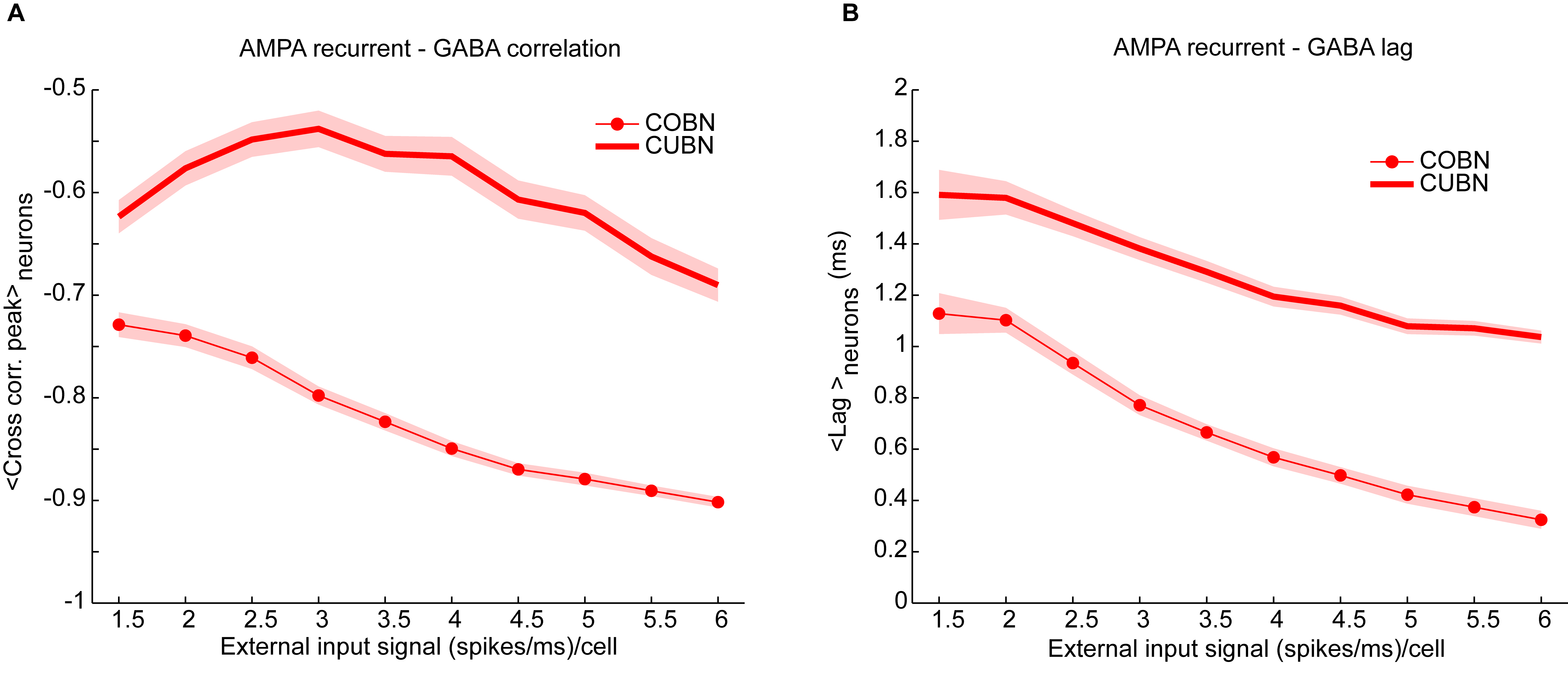
Figure 10: Cross-correlation between AMPA and GABA synaptic currents. Cross-correlation between the time course of recurrent AMPA and GABA currents entering excitatory neurons. (A) Average peak value of cross-correlation between AMPA and GABA input currents into excitatory neurons (see section 8 for details) for CUBN (thick line) and COBN (thin line with markers). Note that, AMPA and GABA currents having opposite sign, the correlation is negative. Shaded areas correspond to standard deviation across neurons. (B) Cross correlation average peak position. This measure quantify how much AMPA inputs lags behind GABA ones. Same color code as (A). Results are computed by using a simulation of 10.5 s per stimulus and show that (i) correlation between recurrent AMPA and GABA input currents is stronger in the COBN than in the CUBN, (ii) input correlation decreases monotonously with input rate in COBN, while it does not in CUBN, (iii) GABA inputs lags behind AMPA inputs by few milliseconds in both networks.

The correlation between AMPA and GABA synaptic currents is known to play a very important role in determining the network dynamics and in particular the spike train variability (Isaacson & Scanziani, 2011). A negative correlation of AMPA and GABA input currents leads to sparse and uncorrelated firing events, while positive values lead to strong bursty synchronized events (Renart et al., 2010). We thus compared the cross correlation between recurrent AMPA and GABA currents impinging on single neurons in COBN and CUBN. We found that the correlation between GABA and AMPA inputs was stronger (i.e., more negative) in the COBN for all external input rates (figure 10A). Moreover, in both networks, AMPA currents led GABA currents with lags shorter than 5 ms, of the order of those observed in (Okun & Lampl, 2008). However, for all external input rates, AMPA-GABA lags were smaller in the COBN (figure 10B). Although figure 10 shows results only for excitatory neurons, similar results held for inhibitory neurons (figure 11). Finally, these results held also when using as external noise a white noise process instead of an Ornstein-Uhlenbeck process (figure 15C).

Figure 11: Correlation between AMPA and GABA inputs to inhibitory neurons. (A) Same as figure 10(A) for inhibitory neurons. (B) Same as figure 10(B) for inhibitory neurons.

6 Cross-neuron correlations

The fact that the cross-neuron variability in average current inputs and MPs was much smaller (figures 7A,D) and high gamma frequency peaks were narrower in the COBN (figures 9A,B) suggested that the activity was more coherent in the COBN than in the CUBN. This view was further corroborated by the finding that the sum of the recurrent currents was larger in the COBN (figure 9F) and suggested that, in this network, input currents may be more correlated across different neurons.

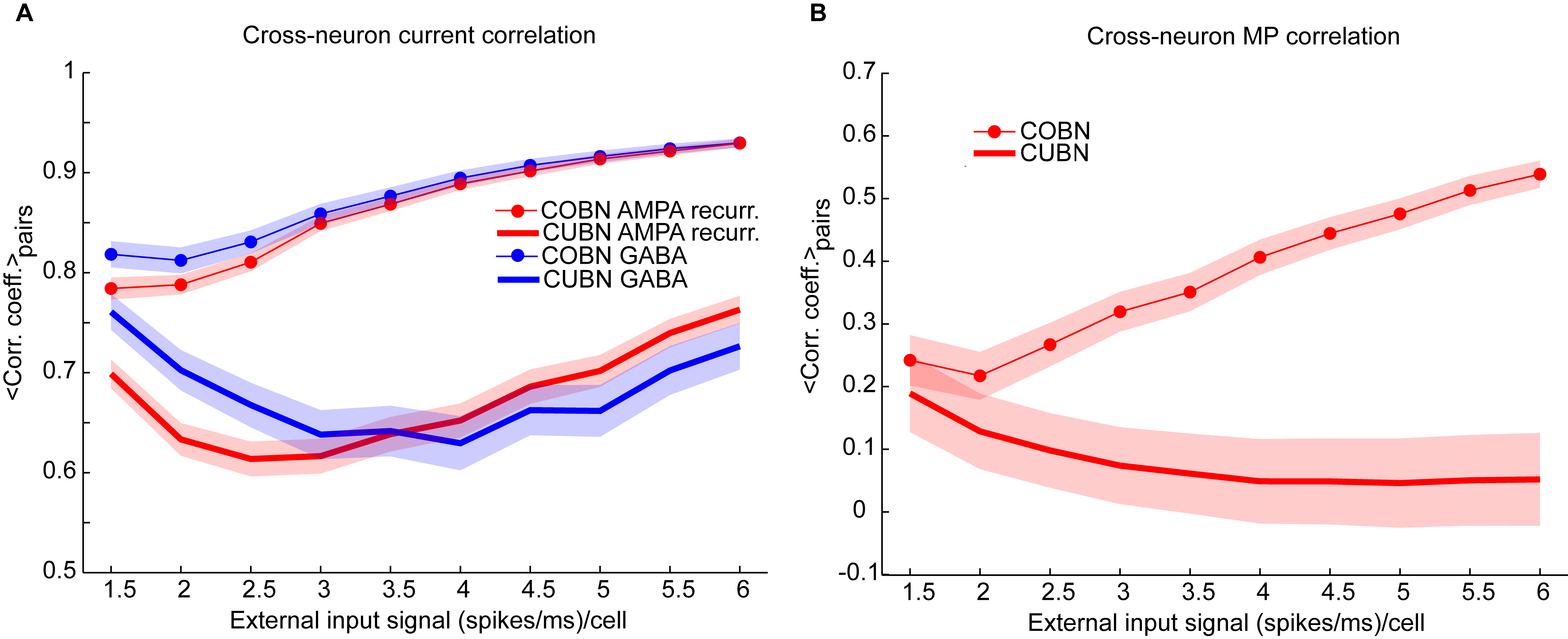
Figure 12: Correlation of the synaptic inputs and of membrane potentials across neurons. (A) Average cross-neuron correlation coefficient between the time course of recurrent AMPA currents (red lines) and GABA currents (blue lines) on excitatory neurons, for CUBN (thick lines) and COBN (thin line with markers), as a function of the external input rate. Similar results hold for inhibitory neurons (see “Rec. AMPA-Rec. AMPA ” and “GABA-GABA ” in table 4). (B) Average correlation coefficient between the membrane potential (MP) time courses of pairs of excitatory neurons as a function of the external input rate. While in the COBN the MP correlation increases with input rate, the opposite occurs in the CUBN. Shaded areas correspond to standard deviation across neuron pairs. Results are computed by using a simulation of 10.5 s per stimulus and show that in COBN the cross-neuron correlations between membrane potentials and between input currents are stronger than in CUBN.

We verified this hypothesis by measuring the average Pearson correlation coefficient between the time evolution of the recurrent AMPA and of the GABA input currents over neuron pairs (see section 8), Figure 12A shows that for both AMPA and GABA currents the average cross-neuron correlation coefficient was indeed significantly stronger (t-test, $p\ll 10^{-10}$) in the COBN for all external input rates. Figure 12A shows also that, in the COBN, the cross-neuron correlation grew with the external input rate for both currents (Pearson correlation test, $p<10^{-5}$). In the CUBN the AMPA currents were linearly correlated to the input rate (Pearson correlation test, $p<0.05$), while GABA currents varied with the input rate in a non-monotonic way. However, if we used white noise, instead of the Ornstein-Uhlenbeck noise (see section 1), the cross-neuron current correlation was again higher in the COBN (t-test, $p\ll 10^{-10}$), but grew monotonously with the input rate for both networks (Pearson correlation test, $p<10^{-5}$), as shown in figure 15A. The increase in the difference between the cross-neuron current correlation in COBN and CUBN with the input rate (figure 12A) led to the increase of the difference in AMPA and GABA total fluctuations in the two networks, shown in figure 9F. To fully appreciate the key role played by correlations note that, if the correlations were similar in COBN and CUBN, fluctuations would be expected to be larger in CUBN since the firing rate was similar for the two networks (figure 8A) and the single PSC amplitude was larger for the CUBN (figure 4).

Figure 13: Membrane potential correlation across neurons. (A) Same as figure 12(B) for pairs composed by an inhibitory and an excitatory neuron. (B) Same as figure 12(B) for pairs composed by two inhibitory neurons.

Cross-neuron correlation of the input currents should be reflected in cross-neuron MP correlation. The previously shown sample traces of the MP of neuron pairs (figures 6E,H) suggested that the correlation was indeed similar for COBN and CUBN in the low-conductance state, but much stronger for the COBN in the high-conductance state. We thus analyzed the average correlation of the MP time courses of pairs of excitatory neurons (figure 12B). Over the whole external input range considered, MP correlation in the COBN was significantly stronger than in the CUBN (t-test, $p\ll 10^{-10}$). Cross-neuron MP correlation in the COBN increased with external input rate (Pearson correlation test, $p<10^{-8}$), while it was only mildly affected in the CUBN (Pearson correlation test, $p<0.02$). These results held for all considered neuron pairs (figure 13) and also when considering white noise, instead of Ornstein-Uhlenbeck noise (figure 15B).

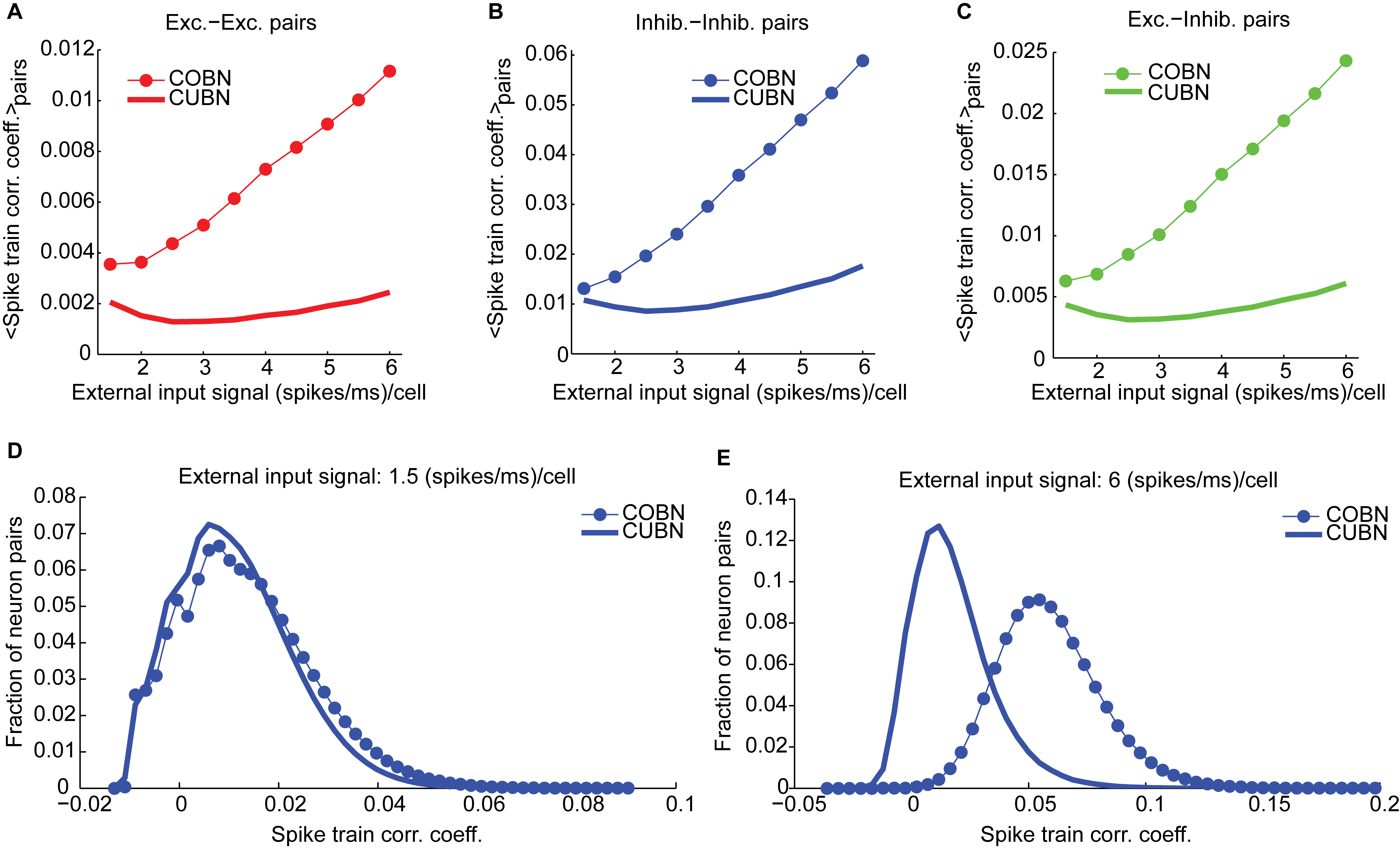
Figure 14: Spike train correlation. Spike train pairwise coefficient of correlation between neurons belonging to the same (A,B) or to different (C) populations. (A) Average spike train correlation between pairs of excitatory neurons as a function of the external input rate for CUBN (thick line) and COBN (thin line with markers). (B) Same as (A) for correlation between pairs of inhibitory neurons. (C) Same as (A) for correlations between pairs composed by an inhibitory and an excitatory neuron. (D) Distribution of the correlation coefficient across inhibitory neurons pairs for an input of 1.5 (spikes/ms)/cell for the two networks. (E) Same as (D) for an input of 6 (spikes/ms)/cell. Note that panels (A–C) do not have error bars for clarity, but the range of correlation values is similar to the one displayed in panels (D,E). Results are computed by using a simulation of 100.5 s per stimulus and show that firing rate correlation is very low for both networks, and it increases with input rate in the COBN, but not in the CUBN.

We finally computed the cross-neuron spike train correlation. We expected it to be related to the MP correlation displayed in figure 12B, even if, since both networks were in a fluctuation-driven state, the spike train correlation should be close to zero (Brunel & Wang, 2003; Renart et al., 2010). We found indeed a very low average spike train correlation (figures 14A–C) such that, for low input rates, a significant fraction of pairs displayed negative correlation (figure 14D).

Figure 15: Correlations in presence of white noise. Same correlation analysis already performed. The difference lies in the fact that here we model the external input noise, n(t), as a Gaussian white noise instead of as an Ornstein-Uhlenbeck process (see section 1). The white noise has the same variance of the OU process used in the main text. (A) Same as figure 12A. (B) Same as figure 12(B). (C) Same as figure 10(A). (D) Same as figure 14(A).

However, in the CUBN, the spike train correlation was weaker and less sensitive to input rate changes than in the COBN (see figures 14A–C and compare figures 14D,E). These results did not change if we injected white noise, instead of Ornstein-Uhlenbeck noise, in the network (figure 15D).

Table 4: Summary of differences between two comparable COBN and CUBN models.

Table 4. Summary of differences between two comparable COBN and CUBN models. This table summarizes our main findings by comparing the values of different features in the COBN used as reference (see table 3) and in the CUBN, when using two constant stimuli: $\nu_{0}$=1.5 and 5 (spikes/ms)/cell. These inputs cause respectively a low-conductance state (LCS) and a high-conductance state (HCS). Values are reported as mean ± standard deviations. PSP peak amplitudes of the COBN are computed by using a spike triggered averaged over 300 neurons from the network in a simulation of 10.5 s (see section 7). The effective membrane time constant of the COBN, $\mathbf{\boldsymbol{\tau}_{eff}}$, the membrane potential, MP, the fluctuations on time of the membrane potential, $\boldsymbol{\sigma_{time}}$(MP) and the coefficient of variation of the ISI, CV ISI, are computed for each neuron and then averaged across neurons by using data from a single trial (of 10.5 s for $\tau_{eff}$, MP and $\sigma_{time}$(MP) and of 100.5 s for CV ISI); the standard deviations are computed across neurons. The average firing rate, FR, the position of the gamma peak of the LFP power spectrum, the current mean and the current fluctuations are computed for each trial (of 4.5 s) considering the activity of all the (excitatory or inhibitory) neurons of the network and then are averaged over 50 trials (the standard deviations are computed thus across trials). The current mean and the current fluctuations refer to the sum of the (AMPA or GABA) currents entering all the excitatory neurons, as indicated by the summation over neurons, $\sum_{n}$, which are exactly the variables used to simulate the LFP. The sum of external AMPA (Ext. AMPA) and recurrent AMPA (Rec. AMPA) is stated as Tot. AMPA. Correlations are computed by using a single trial of 10.5 s. In particular, the cross correlation peak is averaged over the neurons obtained from two randomly selected subpopulations of 200 excitatory and inhibitory neurons (see section 8), while the cross-neuron correlation coefficient is averaged over all the couples of neurons obtained from the same subpopulations (see section 8).

7 Information about external inputs

In the previous subsections we investigated how the average level of spike rate, LFP and spike train correlation depends on the external input to the network, finding a more pronounced stimulus modulation of LFP gamma power and of cross-neural correlation in COBN. To quantify these stimulus modulations of network activity, we computed the mutual information between the stimuli to the network and various aspects of network activity (see for section 9 details).

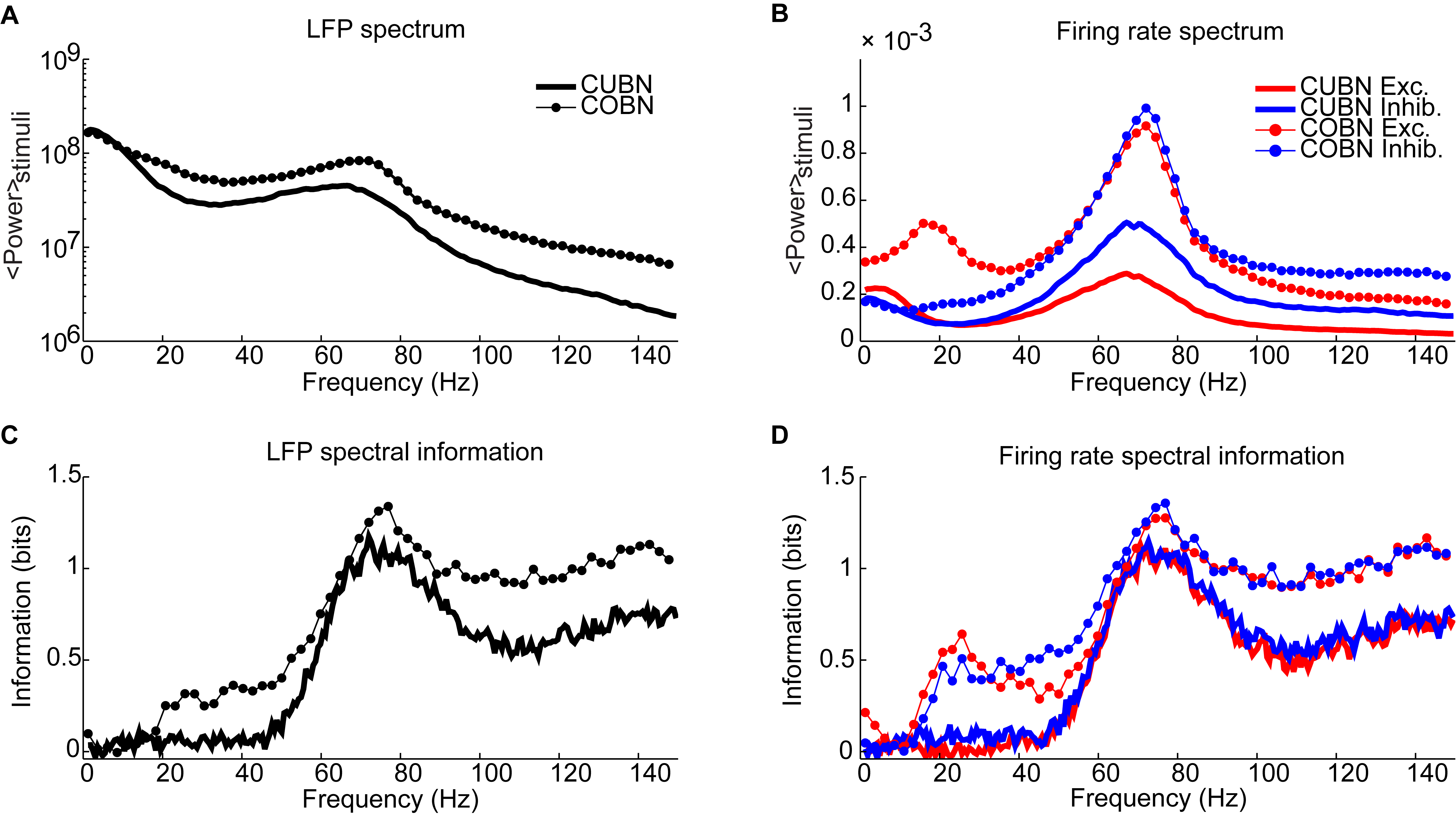
Figure 16: Spectral information relative to the input rate. Information carried by LFP power spectrum (left column) and population firing rates power spectra (right column) about constant inputs ranging from 1.5 to 3 (spikes/ms)/cell with steps of 0.1 (spikes/ms)/cell. Data are obtained by using 50 trials of 4.5 s per stimulus. (A) Average power spectrum of LFP over the entire stimulus range for the COBN and the CUBN (thin line with markers and tick line respectively). (B) Average power spectrum of the total firing rate of excitatory and inhibitory neurons (red and blue respectively) for the two networks [same line code as (A)]. (C) Spectral information carried by LFP about the input rate (see section 9 for details). Same color code as (A). (D) Spectral information carried by total excitatory and inhibitory firing rate about the input rate. Same color code as (B). Results show that the COBN carries more information about constant stimuli for all considered frequencies, both in LFP and in firing rates.

We first measured the information carried by the average firing rate, both of excitatory and inhibitory neurons, in the two networks by using constant stimuli in the range 1.5–3 (spikes/ms)/cell with steps of 0.1 (spikes/ms)/cell. We found that, consistently with the results shown in figure 8A, the information carried by the average firing rate had the same value of 2.3 bits for both neural populations in both network models. Given that the modulation of spike train correlation with external input is greater in the COBN than in the CUBN, we expected that also the mutual information between the spike train correlation and the input rate was greater in the COBN than in the CUBN. Indeed this was the case: information in spike train correlation was much larger in the COBN (1.6 and 2.0 bits for excitatory and inhibitory neurons respectively) than in the CUBN (1.4 and 0.9 bits for excitatory and inhibitory neurons respectively).

We measured then the information content of the LFP power spectrum. The LFP power spectrum averaged over all the presented constant stimuli was higher for the COBN than for the CUBN for all frequencies above 15 Hz (figure 16A). We found that, at all frequencies above 20 Hz, the COBN LFP spectrum carried more information about input rate than the CUBN LFP spectrum (figure 16C). Most notably, the peak information increased by about 20%, and the (20–45) Hz frequency range was informative in the COBN, but not in the CUBN. We repeated the analysis considering the power spectra of the total inhibitory and excitatory firing rate in the two networks. Excitatory neurons in the COBN had stronger power than excitatory neurons in the CUBN for all frequencies (figure 16B, note that here the y-scale is linear, while in figure 16A is logarithmic) and showed a secondary peak at about 20 Hz. For inhibitory neurons, instead, the COBN power spectrum was higher only for frequencies above 15 Hz, as in the LFP .

So far we have investigated only the information carried about the strength of a time-independent input to the network. In a previous work on CUBN (Mazzoni et al., 2008) it has been shown that when the input to the CUBN is dominated by low frequency fluctuation, the network oscillations (captured by both LFP and massed firing rate measures) form two largely independent frequency information channels. A gamma-range information channel is generated by recurrent interactions of inhibitory and excitatory neurons and conveys information about the mean input rate. A low-frequency information channel is generated by entrainment of the low frequency network activity to the slow fluctuations of the input stimulus and carries information about the stimulus time course on such slow time scales. We wanted to test how these two information channels, developed when presenting the network with time-varying stimuli, depended on the choice of the synaptic model.

Figure 17: Spectral information relative to periodic low frequency inputs. Dynamics of the COBN and CUBN when injected with slowly oscillating inputs. The input signals are sine curves with amplitude A = 0.6 spikes/ms and frequency $f$, from 2 to 16 Hz, superimposed to a baseline of $\nu_{0}$ = 1.5 spikes/ms in the left column and $\nu_{0}$ = 5 spikes/ms in the right column. The first baseline value produces a low-conductance state, while the second originates a high-conductance state. Data are obtained from 50 trials of 10.5 s per stimulus. (A,B) LFP power spectrum in the COBN as a function of the external signal frequency. The power spectrum is averaged over trials. (B) Same color code as in (A). (C,D) Same as (A,B) for the CUBN. The inset in (B) shows a detail of the panel in the frequency range where beats are displayed. (E,F) Spectral information carried by the LFP about the frequency of the stimulus presented (see section 9 for details) for COBN (blue line) and CUBN (red line). Results show that the information due to the entrainment of the LFP to the slow input oscillations is almost the same in COBN and CUBN. The only difference is due to the beats that appear in the high-conductance state of the COBN [inset in (B)], which result in a peak of information around 100 Hz (F).

To investigate this point, we injected into the two networks periodic stimuli with fixed amplitude and frequency varying between 2 and 16 Hz. These input frequencies below 16 Hz were taken to represent the slow naturalistic fluctuations present in natural input signals (Luo & Poeppel, 2007; Chandrasekaran et al., 2010; Gross et al., 2013). Since we wanted to investigate potential differences between models separately in low- and high- conductance states, we generated two kinds of input signals: a low-input regime (corresponding to a low-conductance state) and a high-input regime (corresponding to a high-conductance state). Thus the periodic input was made of a sinusoidal signal at a given frequency superimposed to a constant baseline that was set to a low value ($\nu_{0}$ = 1.5 spikes/ms) to induce a low-conductance state and to a high value ($\nu_{0}$ = 5 spikes/ms) to induce a high-conductance state. The amplitude , $A$, of the sinusoidal component of the input was 0.6 spikes/ms across all simulations. Results are reported in figure 17.

We examined first the low-conductance state (left column of figure 17). We considered the LFP power spectra of the two networks in response to periodic stimuli of different frequencies (figures 17A,C). With respect to the previously examined constant input case (figures 9A,B), the LFP power spectrum of both networks had an additional high narrow peak exactly at the same frequency of the periodic input. This peak signaled the entrainment of the network to the periodic input (Mazzoni et al., 2008). The ability of the two networks to entrain their dynamics to the low-frequency stimuli suggested that the power of the LFP at such low frequencies could discriminate which of these periodic inputs was being presented. We tested this suggestion quantitatively by using mutual information, and we found that the slow LFP frequencies conveyed indeed information about the stimuli, approximately in the same amount in both networks (figure 17E). Note that, in the low-conductance state, there was also a slight modulation with the input frequencies of the power in the gamma band (40–70) Hz, with slightly lower gamma power for stimuli of faster frequency (figures 17A,C). These modulations of gamma-range power resulted in moderate amounts of stimulus information in the same range, (40–70) Hz, (figure 17E), and were likely due to the time taken by the networks to develop gamma oscillations following the very low input values occurring at the trough of the sinusoidal input.

Figure 18: Entrainment of LFP to input oscillations. Entrainment of the network oscillations to the frequencies of the periodic input in COBN and CUBN. The input signals are periodic curves as in figure 17, but with frequency $f$ from 2 to 150 Hz. (A,B) Average (over trials) coherence between the phase of the input signal, with frequency $f$, and the phase of the LFP bandpassed in the corresponding frequency range $(f-1,f+1)$ Hz (see section 4 for details). Note that the phase coherence lies in the interval (0, 1). Data are obtained from 50 trials of 10.5 s per stimulus; shaded areas represent standard deviations across trials. Blue lines display results from COBN and red lines from CUBN. (C,D) LFP power spectrum in the COBN as a function of some selected external signal frequencies. The power spectrum is averaged over 50 trials. (D) Same color code as in (C). (E,F) Same as (C,D) for the CUBN. In the low-conductance state both networks entrain very well to the external stimulus, whereas in the high-conductance regime the COBN entrains less well than the CUBN in the middle and in the highest frequency regimes.

We then investigated the high-conductance state (right column of figure 17). Figures 17B,D shows that entrainment of both networks to low frequencies (signaled by the high narrow peak of LFP spectrum at the same frequency as the input) occurred strongly in the high-conductance state. The information about which of these periodic inputs was being presented, carried by the low frequency LFP power, was still identical in the two networks (figure 17F). Moreover, and consistently with the above results obtained with constant inputs (figures 9A,B), the gamma peak in the high-conductance states was much stronger and narrower in the COBN than in the CUBN. Probably because of this, the COBN (but not the CUBN) developed beats of the low-frequency peaks into the frequency range around 100 Hz (inset figure 17B). Since the low-frequency peak varied with the input, these beats led to an amount of information in the COBN LFP power around 100 Hz. The moderate gamma-range information peak, observed in the (40–70) Hz range for the low-conductance state (figure 17E), was absent in both networks for the high-conductance regime (figure 17F), because the input rate was always high at any time point. Thus gamma oscillations in the range (80–94) Hz were always strong, with relatively small fluctuations over time, leading to not discernible modulation across the set of input frequencies considered (figure 17B,D).

We then investigated the ability of the network to entrain to a wider range of input frequencies, in particular including frequencies as fast as or faster than the gamma oscillations intrinsically generated by the network. We did so by testing the network with periodic stimuli over the 2–150 Hz range of input frequencies (figure 18). Again, to investigate differences between models separately in low- and high-conductance regimes, we generated two kinds of input signals that only differed for the value of the baseline, as described above. We quantified entrainment by computing the coherence between the phase of the input signal and the phase of the LFP bandpassed in a narrow band (with 2 Hz bandwidth) centered at the frequency of the periodic input. In the low-conductance state both networks were strongly entrained to the input over the whole range of frequencies examined, as indicated by the high phase coherence (figure 18A). However, when injecting the same input frequencies with the highest baseline (i.e., making the network operate in a high-conductance state), the behavior of the two networks was very different. The CUBN could still entrain extremely well over the entire input frequency range tested. The COBN entrained extremely well to inputs in the (80–94) Hz input frequency range, but less well to inputs with frequency between 16 Hz and 80 Hz, and above 94 Hz. The reason for the presence in the COBN of frequency regions with lower phase coherence (and thus less accurate entrainment to the periodic input) may be because, in the high-conductance state, the COBN had stronger internally generated recurrent oscillations (of higher power than the CUBN, see figures 18D,F) whose dynamics likely did not interfere constructively with the dynamics of the entrainment to the input. This resulted in peaks of less high amplitude in the COBN LFP spectrum at the exact frequency of the periodic input (figures 18D,F). It is interesting to note that the COBN still entrained very well in the (80–94) Hz input frequency range (figure 18B), despite this was also the frequency range exhibiting the strongest recurrent oscillations. Indeed, this range coincided with the peak amplitude of the internally generated gamma oscillations (figure 17B). The ability of the network to entrain well in this gamma range can be understood by observing that this was also the range more strongly modulated by the input rate (figure 9A). Thus, due to their particularly strong responsiveness to the input, external and internal oscillation in this range could interfere constructively, resulting in large peaks of the network LFP at the input frequency (figure 18D).

Figure 19: Spectral information relative to naturalistic stimuli. Information carried by LFP power spectrum (left column) and population firing rates power spectra (right column) about intervals of naturalistic stimulation based on LGN recordings in monkeys watching a movie. Recording time (80 s) is divided into 40 intervals, considered as different stimuli and the information is computed over 50 trials (see section 9 for details). (A) Average power spectrum of LFP over the entire naturalistic input for COBN and CUBN (thin line with markers and thick line respectively). (B) Average power spectrum for the total firing rate of excitatory and inhibitory neurons (red and blue respectively) for the two networks. Same line code as in (A). (C) Spectral information carried by LFP (see Methods for details). Same color code as in (A). In the inset, it is shown the difference between COBN and CUBN information in the low frequency band. (D) Spectral information carried by total excitatory and inhibitory firing rates. Same color code as (B). In the inset, it is shown the difference between COBN and CUBN information in the low frequency band. Results show that, also considering complex stimuli, the information relative to the mean value of the input [that here is the information carried by the frequencies above the delta band, (1–4) Hz] is higher and carried on a broader range of frequencies in the COBN, both in LFP and in firing rates. The information conveyed by delta band frequencies is instead almost identical in the two networks.

To study the differences in the responses of the two networks to stimuli more complex and more biologically relevant than periodic functions, we finally compared the information carried by the LFP and firing rate spectra in COBN and CUBN when using the naturalistic time-varying inputs. We injected then in the networks naturalistic stimuli based on MUA recordings from the LGN of an anesthetized macaque presented with a commercial 80 s color movie clip. The average LFP and total firing rate power spectra for both networks with this set of stimuli are displayed respectively in Figures 14A and B. All these spectra had higher power at low frequencies (as the input signal had), and the gamma peaks were low because the average stimulus rates were in the range 1.2–2 spikes/ms. We computed information about which part of the time-varying naturalistic signal was being presented (see 9 for details). We found that both LFP and firing rates spectra carried more information in the COBN than in the CUBN, for all frequencies (figures 19C,D). The difference in spectral information between COBN and CUBN for frequencies below 5 Hz was almost zero for the LFP and very low for the firing rates (see insets of figures 19C,D).

Our findings therefore confirm that the two independent information channels (one in the low frequencies due to the entrainment to the input, and one in the gamma band due to internally generated oscillations), which were previously reported for the CUBN (Mazzoni et al., 2008), also exist in the COBN. Moreover, our results show that the information about the input conveyed by low frequencies, both in low- and high-conductance states, does not depend on the details of the synaptic model adopted, while the information encoded in the gamma range is larger in the COBN than in the CUBN.

Chapter 3 Relationship between EEGs/LFPs and cell-specific single-neuron firing during slow wave oscillations

In this chapter we investigate how to characterize empirically the relationship between mesoscopic or macroscopic network dynamics and the firing activity of identified single neurons (i.e., neurons belonging to specific classes such as the classes of pyramidal neurons or of interneurons of different types). We address the issue by developing mathematical methods to estimate the linear component of the relationship between firing activity and mass signals and by applying them to concurrent recordings of single-unit firing and of mass circuit activity (LFPs, EEGs) in the neocortex of anesthetized mice in a regime of slow wave oscillations.

1 Introduction

EEGs and LFPs are measures of mass neural dynamics that are easier and more stable to perform than measures of single-neuron spiking activity (Hall et al., 2014). In particular, LFPs are invasive measures that capture mostly postsynaptic potentials (for a full description see 5) typically collecting the activity of populations of neurons located a few hundred micrometers from the recording site (Einevoll et al., 2013). EEG is the extracranial counterpart of the LFP and (like the LFP) captures the mass postsynaptic potentials of large populations of neurons (that are less localized than in the LFP) and it can be measured non-invasively; therefore EEG can be used to monitor neural activity with high temporal precision in healthy humans during cognitive tasks (da Silva, 2013). Practical advantages of EEGs and LFPs over recordings of spiking activity are that (i) LFPs can be recorded more stably for longer periods (ii) their recording requires less power consumption. This is due to the fact the highest power spectral density values of mass signals are found for the lowest frequencies, thus the sampling rates are not required to be high, while spiking activity always needs an high sampling frequency (Hall et al., 2014). However, a difficulty in interpreting these mass (i.e., circuit-level) signals in terms of neural computation is their intrinsic ambiguity: in absence of specific information of how mass signals arise from the individual components that contribute to their generation, it is unclear how they relate to the time course of the underlying spiking activity of neurons in the proximity of the electrode (Einevoll et al., 2013).

Being able to develop simple, yet reasonably accurate, mathematical expressions that relate EEGs or LFPs to spiking activity of single identified cell would be important for several reasons. The estimation of the dynamics of firing of specific classes of neurons from EEGs/LFPs would allow us to correctly infer the underlying neural computations from mass recordings, a feat which is not possible with current computational technologies. With this expression, for example, we would be able to tell, from non-invasive electrical recordings only, that some specific neural classes of interneurons increase or decrease their firing when a subject is performing a certain task, thereby giving quantitative information that we can put into models. The ability of estimating the dynamics of EEGs/LFPs from the spiking activity of individual cell types (the inverse problem of the one just described above) would be valuable to understand how the firing of single cells relates to the circuit “context” which led the neuron to fire, therefore giving precious insights about the way circuits shape single-neuron activity.

Before discussing in more details these topics, it is useful to point out that two different variables can be used to define spiking activity:

• the spike (or firing) rate, FR, (i.e., $r(t)$, see equation 25), which is the average number of spikes in windows of a given amplitude

• the spike times or spike train (i.e., $\rho(t)$, see equation 22), which is the position in time of each spike with a given sampling frequency

Furthermore, as stated above, it also useful to consider the relationship between single-neuron and network-level activities in two opposite directions:

• the direction that goes from single-neuron activity towards mass circuit activity (that we will denote in the following as “spk2EEG/LFP”)

• the direction that goes from mass circuit activity towards single-neuron activity. The latter, in turn, can be measured by the firing rates (“EEG/LFP2FR”) or by the spike trains (“EEG/LFP2spk”)

A series of recent studies has investigated the relationship between mass signals, measured with LFPs/EEGs, and firing activity in different cortical areas and during both stimulation and absence of stimulus (Hall et al., 2014; Musall et al., 2014; Ng et al., 2013; Zanos et al., 2012; Bansal et al., 2011; Okun et al., 2010; Nauhaus et al., 2009; Whittingstall & Logothetis, 2009; Rasch et al., 2009, 2008; Mukovski et al., 2007). In the following, we briefly review the progress made by these studies, and we highlight the questions that these studies left open and that we have tried to address in this thesis.

Whittingstall and Logothetis (Whittingstall & Logothetis, 2009) recorded simultaneously multi-unit activity and EEGs/LFPs from primary visual cortex during visual stimulation. Spectral analysis of EEGs/LFPs recordings reveals that cortical activity presents a reach spectrum of oscillatory activity spread over a wide range of frequencies. Thus they performed a frequency decomposition and focused on the relationship between the network oscillations obtained from LFPs/EEGs and the multi-unit activity in the direction from EEG/LFP to firing rate (i.e., EEG/LFP2FR). In both cases (EEG and LFP), they found that the time course of MUA on a scale of 10-50 ms related statistically both to the delta-band (2-4 Hz) phase and to the gamma-band (30-100 Hz) amplitude of mass signals, with a linear combination of gamma power and delta phase affording more predictability of the multi-unit spike rates than either signal alone. In a second study (Musall et al., 2014), they extended this study by investigating how synchrony between different multi-unit sites relates to EEG amplitude.

Panzeri and colleagues (Mazzoni et al., 2010) developed a network model that provides a detailed mechanistic explanation (both during visual stimulation and during spontaneous activity) of the relationships between activity of excitatory neurons and the phase and amplitude of EEG/LFP rhythms at different frequencies. This modeling accounted well many of the aspects of EEG/spikes relationships observed experimentally by Whittingstall and Logothetis.

In alternative to studying relationships between EEG/LFP networks rhythms and spike times in the frequency domain, Kreiman and colleagues (Rasch et al., 2009) investigated the relationship between multi-unit spikes and LFPs in the time domain during both visual stimulation and absence of stimulus. Their approach was to approximate the LFP time series as a linear convolution of the spike train time series with a temporal “kernel” (i.e., spk2LFP investigation) that describes the spike-field relationship (this “kernel” is similar, though, not identical, to the spike triggered LFP average). This time domain approach is of interest for two reasons. First, if the “kernels” are found to be relatively constant across cells, this approach could be in principle used to estimate the spike rate from the LFP by “deconvolving” the LFP time series with the inverted kernels. Second, these kernels are also useful to describe empirically how LFPs/EEGs are generated within the cortical circuit. Indeed, they are a measure of the spike-LFP/EEG relationship more accurate with respect to the spike-triggered average of the local filed potential, since they discount the confounding factors (in spike-LFP/EEG relationship) that can be given by spatiotemporal correlation of spikes (see section 3). Thus they can be used to estimate, for example, whether the LFP or EEG generation depends on dynamical network parameters such as the cortical excitability (Einevoll et al., 2013).
In another study (Rasch et al., 2008) Logothetis and colleagues estimated the spike trains of MUA (with a sampling frequency of 200Hz) from the LFP (i.e., LFP2spk direction) in monkey primary visual cortex during both visual stimulation and absence of stimulus. They used a support vector machine (SVM) to perform binary classification. The learning algorithm selected a certain number of features (up to 116) of the LFP in order to maximize the estimation performances. The LFP features were obtained both from time and frequency domain and the preferred one is the amplitude of the LFP power fluctuations in the high gamma band (40-90Hz).

Finally, another study (Ng et al., 2013) estimated the similarity between the stimulus selectivity of the firing of auditory cortical neurons in monkeys and the stimulus selectivity that is obtained by EEGs recorded in humans using the same auditory stimuli in both species. The results of this investigation showed that the delta phase is the parameter of auditory cortex EEG that gives decoding and stimulus selectivity closer to the firing of cortical neurons, suggesting that EEG delta phase may be a good proxy for inferring how neurons encode information.

All the above mentioned studies investigate the relationship between LFPs/EEGs and spiking activity of small neuronal populations (or by means of single-unit activity obtained by applying a spike sorting algorithm to MUA signal). A very recent paper (Hall et al., 2014) introduced an important novelty: they examined the effect of using multiple (instead of individual) LFPs to estimate individual firing rate activity and vice versa. However all these works evaluated the firing activity starting from the multi-unit activity. We note that MUA (see section 5) depends on the (extracellular) action potentials of a small group of neurons and does not permit any discrimination of the neural cell types contributing to it, although presumably such recordings capture mostly spikes from pyramidal neurons, because of their larger size and higher number (Logothetis, 2003). Thus:

• previous investigations of the relationship between EEGs/LFPs and firing activity lack a characterization of the cell type from which the firing activity is recorded, and thus cannot reveal the relationship between network-level activity and the firing of specific cell types.

• given that the previous investigations used MUA recordings of spiking activity, and given that MUA has a bias toward measuring pyramidal neurons, these previous investigations cannot tell anything about the relationship between the EEGs/LFPs and the activity of neurons that are not pyramidal cells

As a consequence, previous work failed to show light on how the activity of specific classes of interneurons relate to the EEGs/LFPs. Whether or not such relationships can be detected is made difficult by the fact that inhibitory interneurons, due to their approximately symmetric shape (i.e., star-shaped dendrites), generate a dipole for each spike or synaptic event that is approximately 10 times smaller than that of pyramidal neurons(Murakami & Okada, 2006).

In our work we focus precisely on the relationship between the firing activity of individual genetically-identified interneurons and EEGs/LFPs.

2 Materials and methods

Note that we performed the same analysis for LFP and EEG signal. In the materials and methods section (text and equations), we reported the LFP case, but it is understood that each time you can replace LFP with EEG.

1 In vivo LFP, EEG and two-photon guided juxtasomal recordings

All experiments were performed in mice (25-30 days old) under urethane anaesthesia by Stefano Zucca, Tommaso Fellin and other colleagues in the laboratory of Tommaso Fellin at IIT. These data were kindly provided to me for the present analysis. Details of the experiments are concisely reported below.

PV-Cre (B6;129P2- Pvalbtm1(cre)Arbr/J, Jackson Laboratory, Bar Harbor, USA) and SST-Cre (Ssttm2.1(cre)Zjh/J , Jackson Laboratory, Bar Harbor, USA) transgenic mice were crossed with the TdTomato (B6;129S6-Gt(ROSA)26Sortm14(CAG-tdTomato)Hze/J) reporter line and used for simultaneous recordings of the electroencephalogram (EEG), local field potential (LFP) and single-cell spiking activity. EEG recordings were obtained by placing two epidural stainless steel wires unilaterally at about 3.5 mm distance (in the rostro-caudal direction) from one another. The EEG signal was amplified using an AM-amplifier (AM-system, Carlsborg, WA), sampled at 10 kHz and stored with PatchMaster software. For juxtasomal recordings, patch pipettes (resistance: 4 – 9 MΩ), filled with artificial cerebrospinal fluid solution mixed with Alexa Fluor 488 (20 μM), were lowered through a small craniotomy placed ipsilaterally and in between the two EEG recording sites. Parvalbumin-positive (PV-pos) and Somatostain-positive (SOM-pos) interneurons were identified based on their TdTomato fluorescence in double transgenic mice under the two-photon microscope ($\lambda_{exc}$ = 720 nm). Single-cell spiking activity was recorded with an ELC-01X amplifier (NPI electronic instruments), the signal was sampled at 10 kHz and stored in the computer via PatchMaster software. Simultaneous LFP recording was performed by placing a low resistance glass pipette (0.8 – 1 MΩ) at a distance < 500 μm from the recorded cell. The LFP signal was amplified, sampled and stored in the same way as the EEG signal (datasets: 4 mice, 21 cells for PV-pos and 8 mice, 18 cells for SOM-pos cells).

Figure 1: In vivo two-photon interneuron identification. On the left: schematic representation of the experimental setup. Headfixed anesthetized mice were placed under the two-photon microscope and cells were visualized looking at their fluorescence (λ_exc = 720 nm) through a 40x water-immersion objective (upper part). LFP and SUA recordings were performed by lowering glass pipettes in two small craniotomies closed to each other and indicated by respectively violet and green lines. Cyan lines show the two recording sites for EEG. Right Upper: representation of cortical architecture and experimental configuration: red cells indicate Parvalbumin-positive interneurons; green and violet pipettes display respectively SUA and LFP recording sites. Right Lower: fluorescence imaging showing in-vivo Parvalbumin-positive interneurons identified under the two-photon microscope and a glass pipette (white) placed in close contact for juxtasomal recordings.

2 In vivo LFP and Patch-Clamp recordings

Experiments were performed in PV-Cre mice (25-30 days old) under urethane anaesthesia. For single cell whole cell recordings a patch pipette filled with an intracellular solution (composition in mM: K-gluconate 140, MgCl2 1, NaCl 8, Na2ATP 2, NaGTP 0.5, HEPES 10, phosphocreatine 10 to pH 7.2 with KOH) was lowered through the tissue (depth: from 450 µm to 700 µm) while applying a small positive pressure. Once the cell was reached, a negative pressure was imposed to achieve a stable seal (GΩ) and the membrane was then carefully broken. Pyramidal neurons were identified in current clamp configuration by looking at their spiking activity during depolarizing steps of current injections (Contreras, 2004; Cauli et al., 2000). Single cell membrane potential values were amplified, sampled and stored as the extracellular juxtasomal signals. By positioning a second glass pipette at the same depth of the recorded cell, the LFP was acquired in same conditions as reported above (dataset: 3 mice, 7 cells).

3 Data preprocessing

The recordings are composed by temporal sessions of variable length ($\leq 750$ sec long) which are preceded and followed by a break in the data acquisition. Each cell can have multiple temporal sessions (from 1 to 4) that we divided in segments 240 sec long we call “trials” after discarded an initial transient (from 5 to 20 sec) to avoid any potential border effect. For the PV-pos dataset, this results in a total number of 120 trials. Then we divided each session in segments 240 sec long we call “trials”. Eventually we split each trial into two segments of equal length and in the whole analysis the first 120 sec are used as training set (to compute the Wiener filters and the coefficients of the GLM), while the second half of each trial belonged to the test set and is used to perform the estimation.

All the analysis has been performed using MATLAB (MathWorks). In order to facilitate the computation, LFP signals were decimated to 500 Hz. To detect spike times, firstly we applied a high-pass filter to the mean-subtracted 10 kHz juxtasomal signal (Kaiser filter with zero phase lag and 0.5 Hz bandwidth, very small passband ripple (0.05 dB) and high stopband attenuation (60 dB), cutoff frequency of 100 Hz) and then we applied a detection threshold. Depending on the noise level, the thresholds could vary across temporal series and the median value was 9 SDs of the filtered juxtasomal signal (min=4.5, max=12). Eventually the spike times are downsampled to 500 Hz (like the LFP signal). Note that in this way we obtain the spikes emitted only by the two-photon targeted cell, without need of applying any spike sorting algorithm (because the recordings are juxtasomal).

Traces of the LFP (decimated to 500 Hz) recorded concurrently with the juxtasomal signal is displayed in figure 2, while a typical example of the LFP power spectral density is shown in figure 3.

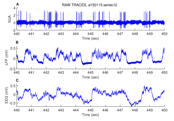
Figure 2: 10 seconds raw traces of simultaneous recordings obtained from three different recording sites. (A) Juxtasomal recording from a PV-pos interneuron. (B) LFP recorded from a glass pipette (at a distance < 500 μm from the recorded cell) and decimated to 500Hz. (C) EEG decimated to 500Hz.

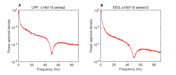
Figure 3: LFP and EEG power spectral density. (A) Typical LFP power spectral density obtained from a temporal series of 750sec. The power density reduction observed around 50 Hz is due to a band-pass filter performed by the amplifier in order to remove artefacts due to electrical equipments. (B) Same as (A) for EEG signal.

Depending on the channel takes as reference, both the LFP and the EEG could have inverted signs. In order to detect the sign, we computed the dependence of the high frequency power (20 90)Hz on the low frequency (0.3 2)Hz phase by means of the cross-frequency coupling of the signal (see figure 4). We then aligned all signals in the same way by reversing the sign of those signals whose cross-frequency coupling had a downward valley at phase value $\pi$ (blue lines in figure 4).

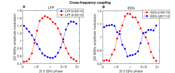
Figure 4: LFP and EEG cross-frequency coupling. Gamma, [20 90]Hz, amplitude modulation of the LFP (A) and EEG (B) signals plotted as a function of their own low delta, [0.3 2]Hz, phases. In particular, cross-frequency coupling is computed as follows. First, we binned into 21 equispaced intervals the range of low delta phase angles from 0 to 2$\pi$, and then in each phase interval we computed the mean gamma amplitude over all data points whose phase belonged to that phase interval: this value is the mean gamma amplitude associated with the given phase interval. Finally, in order to obtain the amplitude modulation, we divided this value by the global mean gamma amplitude (over the whole temporal session, usually 750sec long). When the cross-frequency coupling resulted in a downward valley (blue lines), we inverted the sign of the signal.

Finally we low-pass filtered the LFP (Kaiser filter with zero phase lag and 0.5 Hz bandwidth, very small passband ripple, 0.05 dB, and high stopband attenuation, 60 dB) with a cutoff frequency of 90 Hz.

4 Linear estimation of the time-varying signals

We investigated whether we could linearly estimate the LFP and the EEG from the spiking activity of a single genetically-identified neuron (a PV-pos neuron, with the exception of figure 19), and whether we could estimate the firing activity of a neuron from the mass signals (that it, the “inverse” estimation, see figure 7). We also asked if the estimation is general and robust across cells and animals.

Estimation of LFP and EEG from single-unit spike train

The linear estimation was performed by using the Wiener kernel (see section 3). In particular, when we estimated mass signals from spiking activity (i.e., “spk2LFP”), we defined the spike train (see equation 22) with its mean value, $\rho_{0}$ , subtracted out:

$$\rho(t)=\underset{i}{\sum}\delta(t-t_{i})-\rho_{0}.$$ (1)

According to equation 30, the linear estimation of the (zero-mean) LFP signal had the following expression:

$$\mathrm{LFP_{est}}(t)=\int_{0}^{T}d\tau\>h_{spk2LFP}(t-\tau)\rho(\tau),$$ (2)

where the (trial-specific) Wiener filter see equation 34) was computed as follows:

$$h_{spk2LFP}(t)=\frac{1}{2\pi}\int_{-\infty}^{+\infty}d\omega\>\frac{\tilde{Q}_{spkLFP}(\omega)}{\tilde{Q}_{spkspk}(\omega)}e^{-i\omega t}=\frac{1}{2\pi}\int_{-f_{cut}}^{+f_{cut}}d\omega\>\frac{\tilde{Q}_{spkLFP}(\omega)}{\tilde{Q}_{spkspk}(\omega)}e^{-i\omega t},$$ (3)

where the $\tilde{f}$ indicates the Fourier transform of $f$ and $f_{cut}$ is the cutoff frequency of the LFP. This filter is called “trial-specific” because the cross-power spectral density between the spike train and the LFP, $\tilde{Q}_{spkLFP}(\omega)$, and the power spectral density of the spike train, $\tilde{Q}_{spkspk}(\omega)$, are relative to (the training set of) a single trial. In this way each trial has its own filter. We also considered two other types of Wiener filter with increasing generality: the “cell-specific” filters and the “general” filter. The first filter was computed from and applied to all the trials belonging to a given cell, while the general filter was obtained from and allied to the entire dataset. These filters were computed using the same mathematical procedure used to obtain the trial-specific filter, that is the minimization of the sum of the mean squared errors in the estimation over all the considered trials, as done in (Rasch et al., 2009). Thus, when computing a mean filter, $h^{mean}$, over $N$ trials, we minimized the following quantity:

$$\mathrm{MSD}(\mathrm{LFP,LF}\mathrm{P}_{\mathrm{est}})=\sum_{j=1}^{N}\int_{0}^{T}dt\left[\mathrm{LF}\mathrm{P}_{j}(t)-\int_{0}^{T}d\tau\>h_{spk2LFP}^{mean}(t-\tau)\rho_{j}(\tau)\right],$$ (4)

where $LFP_{j}$ and $\rho_{j}$ are respectively the LFP and the spike train (with the mean subtracted out) of the j-th trial. The explicit expression of the Fourier transform of the mean Wiener kernel takes the following form (see Rasch et al. (2008) for a derivation):

$$\tilde{h}_{spk2LFP}^{mean}(\omega)=\frac{\sum_{j=1}^{N}\tilde{Q}_{spkLFP}^{j}(\omega)}{\sum_{j=1}^{N}\tilde{Q}_{spkspk}^{j}(\omega)}=\frac{\sum_{j=1}^{N}\tilde{Q}_{LFPspk}^{j}(-\omega)}{\sum_{j=1}^{N}\tilde{Q}_{spkspk}^{j}(\omega)}.$$ (5)

Estimation of single-unit firing rate from LFP and EEG

Firing rate computation

We performed a linear estimation also in the opposite direction, that is we estimated single-unit firing rate from the mass signal (i.e., “LFP2FR”). A signal linearly estimated from a continuous (i.e., analogue) signal (such as LFP and EEG) will be in turn continuous. Thus, in order to increase the estimation efficiency, we smoothed the original sequence of spikes in order to obtain a continuous signal we called “firing rate”, FR. This smoothing procedure was performed as follows: first, we averaged the spike train over a rectangular sliding window (i.e., a spike smoothing window, SSW), then we convolved the obtained signal with an Hann window 26 ms wide (Theunissen et al., 2000). Unless otherwise stated, the SSW amplitude was 10 ms.

Wiener Filter

Once we obtained the original firing rate (on the training set), we estimated the FR (on the test set) from the LFP (and in the same way also from the EEG) by using the equation we previously adopted to estimate the LFP from the spiking activity, that is:

$$FR_{\mathrm{est}}(t)=\int_{0}^{T}d\tau\>h_{LFP2spk}(t-\tau)\mathrm{LFP}(\tau),$$ (6)

where

$$h_{LFP2spk}(t)=\frac{1}{2\pi}\int_{-f_{cut}}^{+f_{cut}}d\omega\>\frac{\tilde{Q}_{LFPspk}(\omega)}{\tilde{Q}_{LFPLFP}(\omega)}e^{-i\omega t}.$$ (7)

Analogously to the mass signals estimation, the above equation represents the trial-specific filter. Also in this case we considered the cell-specific and the general filter, which were defined as in equation 5 by substituting “spk” with “LFP” and “LFP” with “FR”.
Note that in order to evaluate how effective was the filter in performing the estimation, we computed also the estimation performances obtained by assuming simply $FR_{est}=LFP$ (without performing any filtering procedure)

General Linear Model (GLM)

In order to evaluate better the results of the FR estimation, we compared the estimation performances obtained by using the kernel with the ones obtained by adopting a general linear model based on frequency decomposition. This model had been used to estimate the MUA firing rate from LFP in a previous work (Whittingstall & Logothetis, 2009), to which we refer for a full description. Briefly, the GLM performs a linear estimation of the true FR by using three regressors: the time resolved power of a given frequency band of the LFP, $Pow_{\mathrm{band1}}$, the instantaneous phase of a given frequency band of the LFP, $Ph_{\mathrm{band2}}$, and a constant term, $k$:

$$FR_{\mathrm{est}}(t)=\beta_{1}Pow_{\mathrm{band1}}(t)+\beta_{2}Ph_{\mathrm{band2}}(t)+k.$$ (8)

The coefficients $\beta_{1}$, $\beta_{2}$ and the constant term, $k$, were computed by minimizing the mean squared difference between the true and estimated FRs (as in the Wiener filter case). The frequency bands used to compute the power and the phase of the oscillations were chosen to maximize the estimation performance (data not shown) among the six traditional EEG bands: delta (<4 Hz), theta (4–8 Hz), alpha (8–15 Hz), beta (15–30 Hz), low (30–60 Hz), and high (60–100 Hz) gamma. In particular, band1 and band2 correspond respectively to the band that had the highest correlation between the oscillatory power and the FR (i.e. [30 60]Hz for LFP and [60 90]Hz for EEG, see panels C,D figure 5) and the highest phase of firing (<4Hz, see panels A,B figure 5, where only the band with the highest phase of firing is displayed).

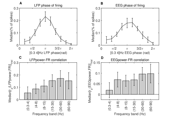
Figure 5: Setting general linear model parameters. We compared the FR estimation obtained by means of a Wiener kernel with the estimation obtained by using a general linear model, as done in (Whittingstall & Logothetis, 2009). This GLM consisted of three regressors: the phase of the slow network oscillations, the power of the gamma network oscillations and a constant term. (A) LFP delta phase of firing. The LFP is bandpassed in the delta band [0.3 4]Hz and the instantaneous phase of the bandpassed signal is computed by means of an Hilbert transform. Then the phase values are binned into 10 equispaced intervals and each spike is assigned to the bin corresponding to the LFP phase assumed when it was fired. (B) Same as (A) for EEG phase of firing. (C) Median Pearson’s correlation between the instantaneous power (extracted by the Hilbert transform) of the bandpassed LFP and the FR. The band used to build the power regressor (i.e., the one that gives the highest performance, data not shown) is the low gamma band, [30 60]Hz. (D) Same as (C) for EEG power; the band used to build the power regressor is the high gamma band, [60 90]Hz. In all the panels median values are computed over the training set and the error bars display the interquartile ranges.

The band-passing procedure was performed by using a Kaiser filter with zero phase lag and 0.1 Hz bandwidth, very small passband ripple (0.05 dB) and high stopband attenuation (60 dB). Then respectively the oscillatory power and phase were obtained as the magnitude and the phase of the Hilbert transform of the band passed signal. Eventually both phase and power were normalized resulting in values between 0 and 1. In particular, the oscillatory power was normalized to its peak value in each single trial. The phase regressor was created by normalizing the instantaneous phase to its peak phase of firing probability in each single trial.

The computation of the GLM was carried out in each single trial, resulting in a “trial-specific” GLM. Analogously to what has been done when performing the estimation by means of the Wiener filter, we also computed the “cell-specific” and “general” GLM by averaging the weights $\beta_{1}$, $\beta_{2}$ and the constant term $k$ across the trials belonging to a given cell and all the trials, respectively.

From firing rate to spike times

From the estimated FR, we extracted the spike times of the neuron by using a non-linear threshold. The FR represents a probability of firing, thus the simplest way to extract spike times relied in detecting a spike each time the FR_est had a local maximum that overcame a given threshold. As a consequence, the value of the threshold determined the number of spikes in the estimated spike train, $\langle FR\rangle_{\mathrm{est}}$. As reference value we used thresholds set to get a number of estimated spikes equal to the number of true spikes; we identified the spike train estimation performed by using this threshold by saying that the $\langle FR\rangle_{\mathrm{est}}$ was “exact” (see for example figure 21). Therefore, in this case, we need to know the true average firing rate in each trial, $\langle FR\rangle_{\mathrm{trial}}$, to obtain the estimated spike train.
In order to quantify if and to which extent the estimation depends on the exact knowledge of $\langle FR\rangle_{\mathrm{trial}}$, we used also a less specific (“general”) threshold (data not shown). In particular, when using the general threshold, the estimated average firing rate takes (no longer the same value as the recorded firing rate but) one out of three possible values which in turn depends on the recorded FR,$\langle FR\rangle_{\mathrm{trial}}$. More precisely these values corresponded to the 17th, 50th and 83rd percentile of the average firing rates distribution (see figure 8) and represented respectively a low, medium and high firing activity for the considered dataset.. The neurons whose$\langle FR\rangle_{\mathrm{trial}}$ fell in the percentile interval (0-33.3) were assigned to the low FR class (with $\langle FR\rangle_{\mathrm{est}}=2.7$ Hz, corresponding to the 17th percentile), the neurons with average firing rate in the percentile interval (33.3-66.6) was assigned to the medium firing rate class ($\langle FR\rangle_{\mathrm{est}}=4.5$ Hz, that was the median) and the other to the high class ($\langle FR\rangle_{\mathrm{est}}=9.4$ Hz, that was the 83rd percentile). In this case, we labeled the spike train estimation by saying that $\langle FR\rangle_{\mathrm{est}}$ was “similar” (to the original one; see figures 23 and 24).
Eventually, in order to investigate more in general the dynamics of the estimation as a function of the threshold, we also analyzed three distinct cases where we adopted a threshold to get respectively the low, medium and high firing activity defined above for all the neurons, irrespective of the original firing rate. We identified these three cases by saying that $\langle FR\rangle_{\mathrm{est}}$ was respectively “low”, “medium” and “high” (see figures 23, 24 and 27).

5 Analysis of cortical datasets

Note that we analyzed all the recordings available without performing any selecting based on the power of slow rhythms.
We divided each trial (240 sec long) into two segments of equal length: the first 120 sec were used as training set to compute the filter, while the second half of each trial belonged to the test set and was used to evaluate the estimation performances (see figure 6).

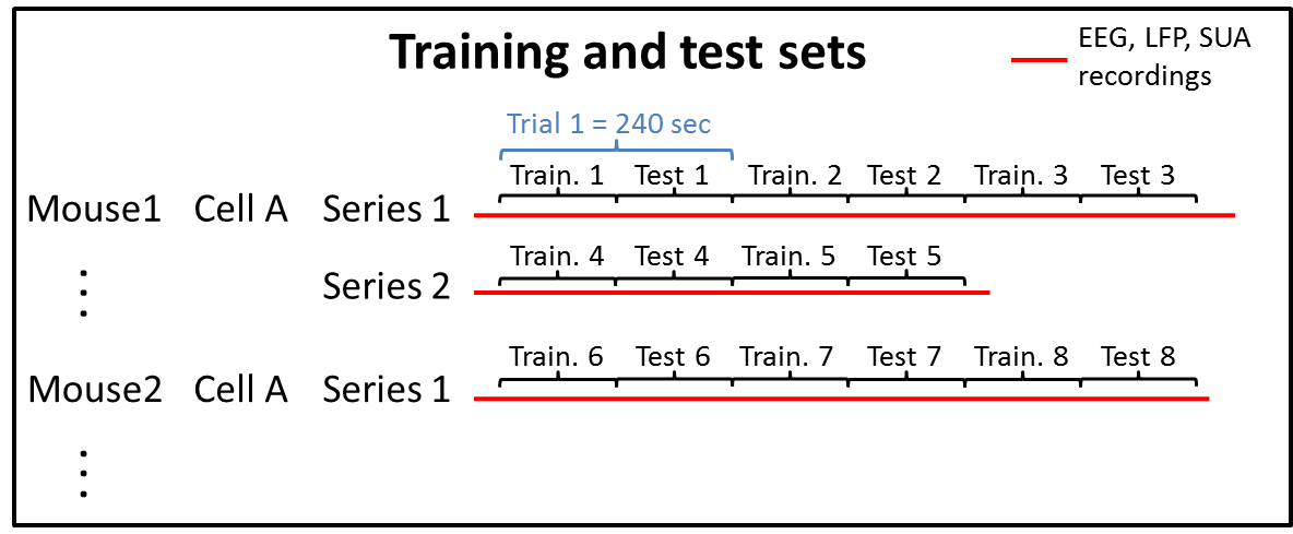
Figure 6: Training and test set division. The original temporal series (red lines) are divided in trials of 240 sec, and then each trial is divided in two equal segments: the first 120 sec are used as training set, while the second half belongs to the test set.

To compute the Wiener filter we estimated respectively the cross-power spectral density and the power spectral density (see equation 33) by using the “cpsd” and the “pwelch” Matlab functions, which performed a Welch’s averaged periodogram method with Bartlett windowing and using nfft = 4096 for both the estimation directions. We also performed the analysis using nfft = 2048 and the results were almost the same (data not shown), since the filters are significant in an interval about 3000 ms wide (see figure 9). Eventually we estimated the inverse Fourier transform needed to obtain the time resolved filter (see equation 34) with the fast Fourier transform algorithm implemented in the “ifft” Matlab function.
We performed the convolution needed to obtain the estimated signal (see equations 2 and 6) in the frequency domain by using the fast Fourier transform implemented in the “fftfilt” Matlab function.

6 Quantification of estimation performance

To quantify the estimation performance of the LFP, EEG and FR estimation we computed the rank Spearman’s correlation between the estimated, $y_{\mathrm{est}}$, and the true signals, $y$, and the normalized mean squared distance, defined as follows:

$$\mathrm{NMSD}(y,y_{\mathrm{est}})=\frac{\mathrm{MSD}(y,y_{\mathrm{est}})}{\sigma_{y}^{2}},$$ (9)

where $\sigma_{y}^{2}$ is the variance of the true signal and the mean squared distance, MSD, is defined in equation 32. NMSD takes values between 0 and 1 with 0 corresponding to perfect estimation and 1 estimation not better than chance level (Gabbiani & Koch, 1998). This is true if $y_{est}$ is the optimal linear estimator of $y$ in the mean square sense. Thus, before computing NMSD, we multiplied $y_{est}$ for the coefficient $k=\sum_{i}[y(t_{i})\cdot y_{\mathrm{est}}(t_{i})]$ /$\sum_{i}y_{\mathrm{est}}^{2}(t_{i})$, which minimizes the MSD between $y$ and $y_{\mathrm{est}}$. In particular, when evaluating the FR estimation performances, we rectified the estimated FR before computing Spearman’s correlation and NMSD.
To assess the statistical significance of the LFP estimation, we compared the performance distribution with the one obtained under the null hypothesis where the Wiener kernel, $h_{spk2LFP}^{\mathrm{rand}}$, conveyed no information about the relationships between the temporal structure of spike trains and LFP time courses. More specifically, for each training trial, we generated a Poisson spike train with the same average firing rate as the true spike train. We then computed the Wiener filter $h_{spk2LFP}^{\mathrm{rand}}$ (that could be trial-specific, cell-specific or general depending on the original filter we were testing) as in equation 3 (or 5) by minimizing the MSD between the true LFP and the one estimated from the Poisson spike train. Eventually we used the random filter to estimate the LFP:

$$\mathrm{LFP}_{est}^{\mathrm{rand}}(t)=\int_{0}^{T}d\tau\>h_{spk2LFP}^{\mathrm{rand}}(t-\tau)\rho(\tau).$$ (10)

We repeated this procedure performing 50 different realizations of the Poisson spike train for each trial and then we averaged the estimation performance over the 50 realizations to obtain the average random performance distribution used as null hypothesis. If the filter conveys no information about the relationship between the temporal structure of spike trains and LFP time courses, we would expect the estimation performance of the estimated LFP to be close to the ones obtained from the random filter.

To quantify the performances when estimating the spike times we need to introduce a parameter, dt_accuracy, that we use to resample the spike trains. Note that we count the number of spikes in each time window dt_accuracy, thus the value of the resampled spike trains in each dt_accuracy can be higher than one. We then compared the number of spikes in each dt_accuracy window in the true and estimated spike trains by measuring the sensitivity and the precision of the estimation. In particular, sensitivity is defined as follows

$$\mathrm{Sensitivity}=\frac{TP}{TP+FN},$$

while precision is

$$\mathrm{Precision}=\frac{TP}{TP+FP}.$$ (11)

TP (true positive) is the number of estimated spikes that fitted true spikes, FN (false negative) is the number of true spikes that do not have corresponding estimated spikes and finally FP (false positive) is the number of estimated spikes that do not have corresponding true spikes. Note that this computation/comparison is performed step by step in each dt_accuracy. Thus the sensitivity measures the percentage of the true spikes that are correctly estimated within time windows dt_accuracywide, while the precision is the percentage of the estimated spikes that correspond to true spikes. Note that if the true and the estimated spike trains have the same number of spikes (as in the case where $\langle FR\rangle_{est}$ is exact, see section 4), $FN=FP$ therefore $\mathrm{Sensitivity}=\mathrm{Precision}$.
To assess the statistical significance of the spike train estimation, we considered two different null hypotheses. The first is given by the estimation performances obtained from a Poisson spike train having the same average FR of the estimated spike train. (The Poisson process is a point-like process that generates spike times with a given probability at any given time, independently of spikes emitted at earlier or successive times). For each trial we performed 50 different realizations of the Poisson spike train and we took the average performance. This null hypothesis is labeled as “Poisson” in figures 23 and 24 and it quantifies the performance only due to the knowledge of the average firing rate (independently on the relationship between firing activity and LFP). The second null hypothesis is obtained by the estimation performances obtained randomly placing the estimated spikes in the intervals where the estimated FR is above the spike-detection threshold (see section 4). For each trial we repeated this procedure 50 times and we took the average performance distribution. This null hypothesis is labeled as “Shuffled” in figures 23 and 24 and it analyzes if the estimated spikes are placed at random level where the FR_est is above the spike threshold.

All the performance measurements we adopted do not depend on the magnitude of the signals. Nevertheless, when computing mean Wiener filters (see equation 5) and mean GLM, the involved signals had to have the same units across trials. In particular, the firing activity was in units of (spikes/dt_sampling, where dt_sampling= 2 ms) and the LFP were in standard deviations units (s.d.u.).

3 Results

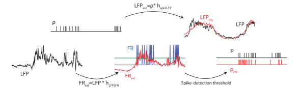
Figure 7: Schematic of the analysis performed. We linearly estimated the signals by means of Wiener kernels and we quantified how robust the estimation is by comparing the performances obtained by trial-specific, cell-specific filters and also when using a unique filter for all the mice. Top: the estimated LFP/EEG is obtained by convolving the relative Wiener filter, $h_{spk2LFP/EEG}$ with the spiking activity, $\rho$, of single (both excitatory and inhibitory) neurons. Bottom: firstly, the FR is estimated by convolving the LFP (or the EEG) with the Wiener kernel, $h_{LFP/EEG2FR}$, then a spike-detection threshold is applied to detect spike times. We compared this estimation with the ones performed when (i) avoiding the convolution with the filter (i.e., by applying the threshold directly to the LFP/EEG) and (ii) estimating the FR by means of a general linear model based on frequency decomposition of the mass signals used in (Whittingstall & Logothetis, 2009).

While mass measures of circuit activity (as EEGs and LFPs) are analogue signals, spike can be considered as point-like processes. Linear estimation methods of analogue signals from point-like processes rely on some kind of filtering operation on the sequence of times when the point-like is present. Thus, the number of available spikes is crucial when performing such a kind of estimation of mass signals. In particular, in our datasets the spiking activity comes from single genetically-identified (i.e., PV-pos) interneurons (see section 1), thus the firing activity of the identified population of neurons is very important. In figure 8, we showed the distribution of the average firing rates of the single PV-pos interneurons. These neurons are fast-spiking neurons and this is the reason why we chose them, with respect to the SOM-pos interneurons, which had an extremely low firing activity (see figure 19).

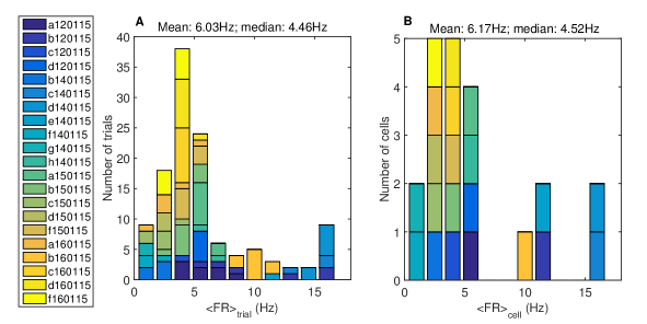
Figure 8: Distribution of the average firing rates across trials (240 sec) (A) and cells (B). The legend shows the cell the data belong to. Mean and median values of the distributions are displayed in the panel’s titles.

1 Estimating LFP and EEG from SUA

We performed a linear estimation of both the EEG and the LFP recorded in layer 2 of neocortex of mice under anesthesia from the concurrently recorded spiking activity of a single PV-pos interneuron (in layer 2) placed at a distance <500 μm from the LFP pipette. We then extended this analysis (see figure 19) by also including spiking activity recorded from either a SOM-pos interneuron in layer 2 and a pyramidal neuron in a deep layer (i.e., 5 or 6). The estimation was done by means of the (first order) Wiener kernel, as described in equation 2. In order to investigate if and to which extent the estimation algorithm could be generalized, we considered three kinds of filters, with increasing generality: trial-specific, cell-specific and general filters.

The general filter obtained for respectively the LFP and EEG estimation is showed in figure 9 panels (A) and (B), where also the spike-triggered averages are displayed.

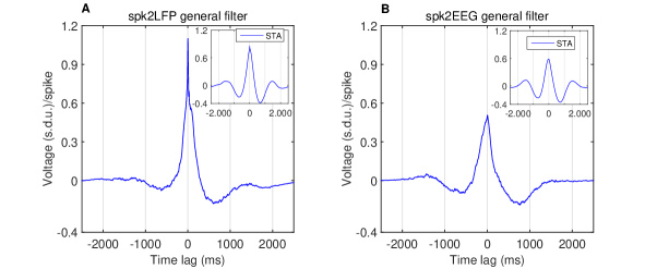
Figure 9: General Wiener kernels for LFP and EEG estimation. (A) Mean filters (over all the trials) used to estimate the LFP from the spiking activity of a PV-pos interneuron. The peak is at 2 ms lag. The inset, which has the same axes than the main panel, shows the LFP spike-triggered average as term of comparison (see section 3). (B) Same as (A) for EEG estimation. The peak is at 6 ms lag.

The LFP (and EEG) estimation is obtained by placing a series of filters centered on the spike times and then summing them up. Therefore, the time lag associated with the filter peak (2 ms for LFP and 6 ms for EEG) indicates the delay where in average there is the strongest relationship between mass signal fluctuations and firing activity. Thus, for example, the average strongest effect of a spike will be observed on the LFP 2 ms after the spike emission. Furthermore, the higher and tighter value of the filter peak when estimating the LFP is an indication of the fact that the relationship between firing activity and LFP is closer and more stable than in the EEG case. Note that these filters are acausal (indeed we do not know whether spikes cause directly the mass signal, for example because the spikes generate a dipole directly captured by the mass signal, or whether the network oscillations cause the spike times, for example because the network oscillations suppress or enhance the likelihood of an individual cell firing at given phase of network oscillation Einevoll et al. 2013). This means that each spike affects the estimated LFP in time steps both preceding and following the spike emission. In particular, the values of the filter for respectively positive (negative) time lags shows the contributions to the LFP_est of each spike after (prior to) its emission. In figure 10 we show a representative example of both the LFP and EEG estimation obtained from the same spiking activity by using the filters displayed in figure 9.

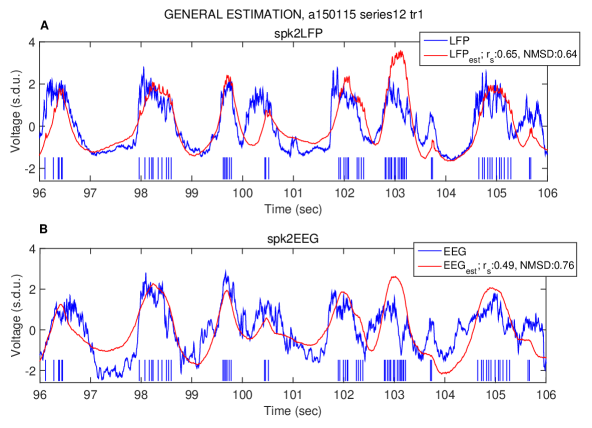
Figure 10: LFP/EEG estimation example when using the general filters (showed in figure 9). (A) 10 seconds trace of the recorded LFP (blue) compared with the estimated one (red). The latter is obtained by convolving the spike train (blue vertical lines) with the (general) Wiener kernel. The estimation performances (i.e., Spearman’s correlation and normalized mean squared distance between LFP and LFP_est) on the whole test set are displayed in the legend. (B) Same as (A) for EEG estimation. Note that the examples in panels (A) and (B) are taken from the same trial and their estimation performances (and $\langle FR\rangle=4.9$Hz) are close to the median performances over the entire dataset.

We measured the estimation performance by means of the Spearman’s correlation, $r_{s}$, and of the NMSD between the original and estimated signals on the test set (see section 6). In figure 11 we show the distribution of the Spearman’s correlations across trials and cells both for LFP, panels (A,B), and EEG estimation, panels (C,D). We found that the performances vary on a broad range being relatively similar for trials belonging to the same cell (both for LFP and EEG, compare panels (A,C) with (B,D) in figure 11); nevertheless, the ranked performances differed when comparing LFP and EEG estimation (data not shown), suggesting that the relationship between FR and mass signals does not only depend on the average firing rate of the neuron, but it also depends on the nature and signal to noise ratio of the mass signal.

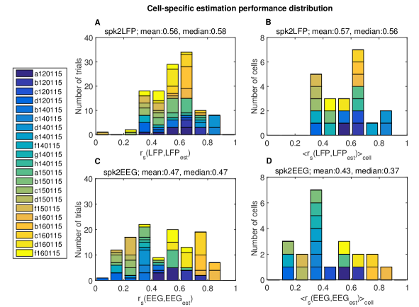
Figure 11: Distribution across trials and cells of LFP and EEG estimation performances. (A) Distribution across trials of the LFP estimation performances (as measured by Spearman’s correlation), when using the cell-specific filter; mean and median values are displayed in the panel’s title. (B) Same as (A) for the distribution of the average values across cells. (C,D) Same as respectively (A,B) in case of EEG estimation. The legend indicates the cells the data belong to.

When using cell-specific filters, the median values of $r_{s}$ for LFP_est across all the trials is 0.58$\pm$0.12 (median$\pm$interquartile range/2, n=120 trials) and NMSD=0.70$\pm 0.12$, while, for EEG_est, $r_{s}$=0.47$\pm$0.18 and NMSD=0.78$\pm$0.17.

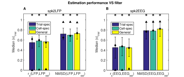
Figure 12: LFP and EEG estimation performance VS filter specificity. (A) LFP estimation performances as a function of the kind of kernels used; the colored bars indicate the median values (and the error bars the interquartile ranges) over the test set. The diamonds are the median values over the training set; the triangles represent the median estimation performances (on the test set) under the null hypothesis, that is when using the random filter, $h^{\mathrm{rand}}$ (see section 6). * $p\ll 10^{-10}$ based on a one-tailed Kolmogorov-Smirnov test comparing the estimation performances against the null hypothesis performances. (B) Same as (A) for EEG estimation.

Note that the performance distributions obtained from both the trial-specific and general filters are never significantly different from the cell-specific one, (according to two-tailed Kolmogorov-Smirnov tests where respectively p>0.37 (0.29) when comparing Spearman’s correlation for LFP (EEG) estimation), as summarized in figure 12. Therefore the estimation is robust with respect to the kernel’s generality, suggesting that the relationships underlying the estimation reflect general and robust network phenomena under the experimental conditions considered and that the algorithm does not express any kind of overfitting of trial-specific features.

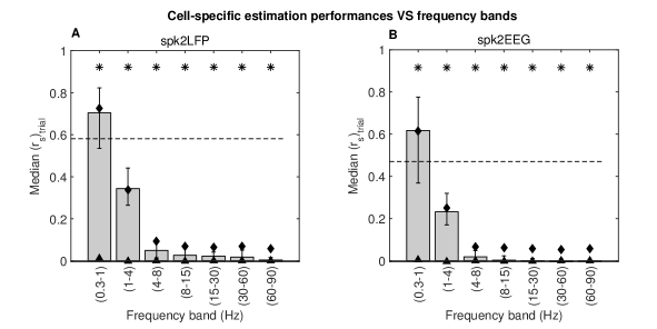
Figure 13: LFP and EEG estimation performance VS frequency bands. (A) LFP estimation performance as a function of the frequency bands; First, both the LFP and the LFP_est have been filtered in the specified frequency band, then the Spearman’s correlation between the two filtered signals has been computed. The gray bars indicate the median values over the test set, while the error bars represent the interquartile ranges. The diamonds are the median values over the training set, while the triangles represent the estimation performances (on the test trial) under the null hypothesis (as in figure (12)). The horizontal dashed line indicates the median value for the unfiltered LFP. * $p\ll 10^{-10}$ based on one-tailed Kolmogorov-Smirnov test comparing the estimation performances against the null hypothesis performances. (B) Same as (A) for EEG estimation; * $p\ll 10^{-6}$. The showed performances are obtained by using a cell-specific kernel; similar results are obtained when using both trial-specific and general kernels (data not shown).

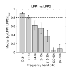
Figure 14: Comparing two LFP traces recorded at the SUA-LFP pipette distance. The same analysis done in figure 13 is applied here to evaluate the frequency-dependent similarity between two LFP traces recorded at a distance < 500 μm. Note that this is the same distance present between the pipettes used to record the LFP and the SUA analyzed in all the other figures. The horizontal dashed line indicates the value for the unfiltered LFP (that is 0.80$\pm$0.05 (median$\pm$interquartile range/2), while for the NMSD is 0.36$\pm$0.05, datum not shown). Each trial lasts 100 sec (3 mice, 31 trials).

To understand which components of network oscillations are better captured by our model, we analyzed how the performances are distributed across the frequency spectrum of LFP_est and EEG_est. We found (figure 13) that our linear estimation reconstructed better the low frequency components of the signals, even if the performances remains significantly higher than random level for the whole spectrum. This is intuitively expected for two reasons. The first is that the estimation (especially a linear one) will tend to reconstruct better the oscillations with largest amplitudes, which are in the lowest frequency band (see figure 3). The second reason is due to the experimental setup. Indeed, the pipette used to record the spiking activity is placed at a given distance (<500 μm) from the pipette used to record LFP (and also from the wires used to record EEG), thus we use the SUA recorded at a given place to reconstruct a LFP recorded some hundreds micrometers away. As a consequence, the LFP performance estimation depended also on the spatial synchrony of LFP oscillations, which is higher for lower frequencies, as shown in figure 14, where we compared two LFP traces recorded at the distance usually present between LFP and SUA pipettes.

To gain a deeper insight about the parameters shaping the relationships between single-neuron spiking activity and mass signals, we investigated how the correlations between original firing rates and network oscillations (figures 15 and 16) affect the estimation performance dynamics.
To assess how the FR of single cells is synchronized with the mass signal, we computed the Spearman’s correlation between FR and mass signal time courses. We found that the median correlation between the FR and the LFP (0.28) is higher than the one between FR and EEG (0.22); this is not surprising since the EEG is a signal integrated over a broader area than the LFP. Nevertheless, what is more important is that, in the LFP case, there is an high positive Pearson’s correlation between the average firing rate and the synchronization between FR and LFP ($r_{p}=0.87$), which is strongly attenuated in the EEG case ($r_{p}=0.36$, compare panels (A,B) in figures 15 and 16). This means that, in the LFP case, the higher the average firing rate, the higher is the synchronization of firing activity with the mass signal, whereas, in the EEG case, this is not as clear. This is the crucial point to understand the differences in the way the estimation performances are shaped in the LFP and EEG case throughout this analysis and, in particular, it is the reason why we observed a strong correlation between the average firing rate and the LFP estimation performances (see panels (A,B) in figure 17), which is absent in the EEG estimation (see panels (A,B) in figure 18).
We also investigated if the average firing rate is related to the power of slow frequencies ([0.3 2]Hz) of the LFP and EEG. We found weak correlations between these two variables both for LFP and EEG (see panels (C,D) in figures 15 and 16): the average firing rate is only weakly dependent on the power of the slow network oscillations. However, note that our recordings are performed in a regime of slow wave oscillations, where the slowest frequencies are always the largest in amplitude (see figure 3) and their power variation across trials is smaller than the variation observed in the average firing rates.

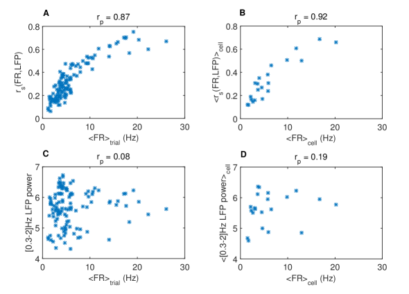
Figure 15: Relationships between firing rate and LFP in the test set. (A) Spearman’s correlation between the LFP and the concomitant firing rate, $r_{s}(\mbox{FR,LFP})$, as a function of the average firing rate. The firing rate is computed by using a spike smoothing window of 50ms (see section 4). The median value of $r_{s}(\mbox{FR,LFP})$ over all the trials is 0.28. (B) Same as panel (A) for the average values in each cell. (C) Scatter plot between the average FR and the power spectrum of the low LFP delta band [0.3 2]Hz; each point represents the values in a trial. (D) Same as panel (C) when each point represents the average values over the trials of a cell. The Pearson’s correlations between the plotted variables are displayed in the panels’ titles.

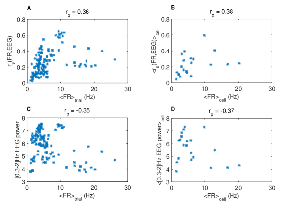
Figure 16: Relationships between firing rate and EEG in the test set. Same analysis performed in figure 15. (A) Spearman’s correlation between the EEG and the concomitant firing rate, $r_{s}(\mbox{FR,EEG})$, as a function of the average firing rate. The median value of $r_{s}(\mbox{FR,EEG})$ over all the trials is 0.22. (B) Same as panel (A) for the average values in each cell. (C) Scatter plot between the average FR and the power spectrum of the low EEG delta band. (D) Same as panel (C) when each point represents the average values over the trials of a cell.

As a consequence of the fact that the oscillations estimated better are the slowest ones (see figure 13), we could expect to find a positive correlation between the estimation performance and the power of the lowest frequencies. On the other hand, another crucial variable is the number of spikes available to reconstruct the signal, that is the average firing rate. Therefore, we will focus on the contributions of slow network oscillations and average firing rates in shaping the estimation performances. Interestingly, when looking at the scatter plots of the performances with respect to those two variables, we found that the highest correlation is with the average firing rate for LFP estimation ($r_{p}=0.66$, see figure 17) and with the low frequency power for EEG estimation ($r_{p}=0.59$, see figure 18). This asymmetry is due to the differences in the relationships between FR and LFP with respect to FR and EEG pointed out in figures 15 and 16. Indeed, the estimation is enhanced (i) by high average firing rates, but, importantly, only if the firing activity is synchronized with the mass signals and (ii) by large amplitudes of slow oscillations. For what concerns the contributions of the average firing rate, the correlation between average firing rate and (mass signal-FR) synchronization is stronger for LFP ($r_{p}=0.87$) than for EEG ($r_{p}=0.36$). Thus, when a neuron has an high firing activity, this activity is strongly synchronized with LFP, but much less with EEG. In addition, the average FR tend to decrease when increasing the EEG low frequency power ($r_{p}=-0.35$), therefore, in case of EEG estimation, the performances are almost independent on the average firing rate (see panels (A,B) figure 18). As a consequence, the EEG estimation performances are mainly determined by the amplitude of slow oscillations (see panels (C,D) figure 18). On the other hand, in our regime (i.e., slow wave oscillation), we have always large amplitude values of the slowest network oscillations thus (as stated above) their power is relatively stable across trials while the variation observed in the average firing rates is wider. The larger variability of the average FRs, combined with the fact that LFPs are strongly synchronized with high FR activities (as stated above), results in an higher correlation between performances and average FRs with respect to the one between performances and LFP low power (compare panels (A,B) with (C,D) in figure 17).
In panels (E,F) of figures 17 and 18, we show the correlation between the performances and the average FR multiplied by the low frequency power. In the EEG case, the resulting correlation is smaller than the correlation between the performances and the variables taken individually, because FRs and mass signals are not synchronized and thus an high firing rate does not improve the performances. On the other hand, in the LFP case, the correlation in panels (E,F) is (slightly) larger than in the other panels confirming that, when FRs and mass signals are synchronized, both slow network oscillations and FR enhance estimation.

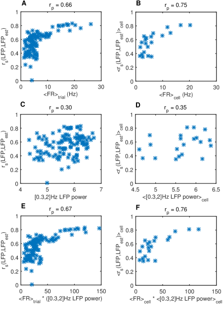
Figure 17: LFP estimation performance scatter plots. (A) LFP estimation performance in each trial (as measured by Spearman’s correlation) as a function of the average FR. (C) LFP estimation performance of each trial as a function of the true LFP power spectrum in the low delta band, [0.3 2]Hz. (E) LFP estimation performance of each trial as a function of the product between the true low LFP power spectrum and the average FR. (B,D,F) Same as respectively (A,C,E) when each variable is averaged over the trials belonging to a cell. The Pearson’s correlations between the plotted variables are displayed in the panel’s titles. The showed performances are obtained by using a cell-specific kernel and similar results are obtained when using both trial-specific and general kernels (data not shown).

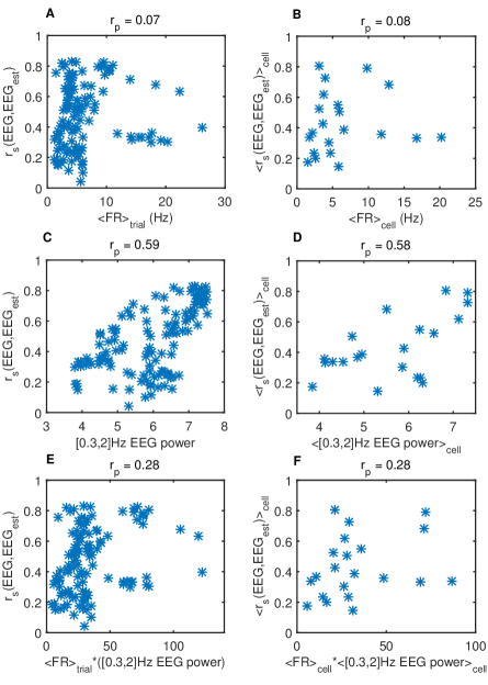
Figure 18: EEG estimation performance scatter plots. Same analysis performed in figure 17. (A) EEG estimation performance of each trial as a function of the average FR. (C) EEG estimation performance of each trial as a function of the true EEG power spectrum in the low delta band, [0.3 2]Hz. (E) EEG estimation performance of each trial as a function of the product between the true low EEG power spectrum and the average FR. (B,D,F) Same as respectively (A,C,E) when each variable is averaged over the trials belonging to a cell. The Pearson’s correlations between the plotted variables are displayed in the panel’s titles. The showed performances are obtained by using a cell-specific kernel and similar results are obtained when using both trial-specific and general kernels (data not shown).

In summary, we found that the performance of LFP and EEG estimation depends mainly on two distinct features: (i) the amplitude of low frequencies in the mass signal and (ii) the number of spikes available to reconstruct the signals (i.e., the average firing rate of the cell). Both of them, when increasing, tend to facilitate the estimation. Since the recordings are performed during slow wave oscillations, we remain always in a regime where the slowest frequencies are largest and their power is relatively stable across trials. On the other hand, the average firing rate can span a broad spectrum of values, thus its fluctuations are wider than the variations of LFP and EEG low power. As a result, when the firing activity is synchronized with the mass signals, as happens with the LFP, the average FR will prevail in shaping the estimation performances, otherwise, the level of low frequency oscillations will mainly determine the performances (EEG case).

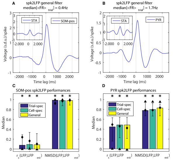
Figure 19: LFP estimation from the firing activity of SOM-pos interneurons and pyramidal neurons. Results from the analysis of other two datasets are shown. (A) General Wiener filter used to estimate the LFP from the spiking activity of an individual SOM-pos interneuron (8 mice, 18 cells and 99 trials). The peak is at 52 ms time lag. As in figure (9), the inset displays the LFP STA. Note that the median firing activity of this kind of neurons is very low: median average FR equal to 0.4 Hz (see figure (8) for comparison with the PV-pos activity). (B) Same as (A) when the firing activity comes from a single pyramidal neuron of deep layers (3 mice, 7 cells and 23 trials). Filter peak located at 118 ms time lag. (C,D) As done in figure (12), we show the performances and their significance against the null hypothesis as a function of the filter used when estimating the LFP from the firing activity of a SOM-pos (C; * $p<0.004$) and of a pyramidal neuron (D; * $p<10^{-5}$).

We conclude this analysis by summarizing some preliminary results of the application of our analysis to other two datasets where the mass signal is measured only as LFPs and the SUAs come respectively from Somatostatin-positive interneurons in layer 2 and excitatory pyramidal neurons from a deep layer (i.e., 5 or 6) in mouse neocortex. In the first case, the firing activity is extremely low (median[$\langle FR\rangle$]=0.4 Hz, indeed this interneurons are no longer fast-spiking), and this leads to a fall in the estimation performances (panel (C) in figure 19). For the excitatory neurons, even if the average firing rates decrease considerably with respect to PV-pos (median[$\langle FR\rangle$] from 4.5 Hz to 1.7 Hz), the performances remain quite high (panel (D) figure 19) suggesting the existence of a strong lock between pyramidal firing activity and mass signal. Finally, when looking at the correlations of the estimation performances with average firing rates and powers of the slow LFP oscillations, we found results very similar to the ones showed in figure 17 for the PV-pos interneurons (data not shown).

2 Estimating SUA from LFP or EEG

In this section we reverse the direction of the estimation, as we attempt to estimate SUA from from mass signals. This analysis is important to understand how we can infer the changes in firing rates of specific cell types in cases (such as those in human cognitive experiments with EEGs) when it is only possible record mass signals. We performed this estimation in two steps: first, the linear estimation of the FR, through convolution with a Wiener kernel, second, a non-linear threshold to detect the estimated spikes. We evaluated how the performances depend on the specificity of the filter (as done for the estimation in the opposite direction), on the spike-detection threshold and we also compared the performances obtained by using the Wiener kernel with the ones obtained by considering other two models of the estimated FR.

Spike train estimation

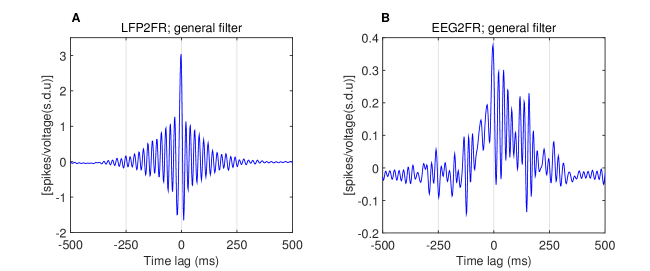
Figure 20: General Wiener kernels for FR estimation from LFP and EEG. Mean filters (over all the trials) used to estimate the FR (spike smoothing window of 10 ms) of a PV-pos interneuron starting from the LFP (A) and from the EEG (B) signals. In panel (A) the filter peak is at -2 ms and in panel (B) at -4 ms.

The mean Wiener kernel over all the dataset is shown in figure 20 for both LFP and EEG cases. Each point of the filter represents the weight given to the LFP (EEG) signal in $(t^{*}+\mathrm{time\>lag)}$ when estimating the FR in $t^{*}$. The filters have oscillations narrower with respect to the filters used to estimate mass signals (figure 9) and this reflects the fact that the FR itself displayed very narrow oscillations (which identify the spikes position, see figure 21). Note that the EEG2FR filter is much smaller than the LFP2FR one; this indicates a weaker synchronization between firing activity and the EEG oscillations. As expected, the time lags associated with the filter peaks have inverted sign with respect to the case where the estimations were performed in the opposite direction.

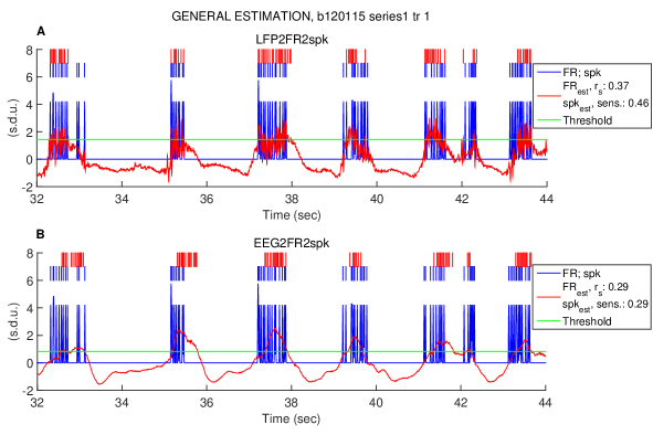
Figure 21: Example of spike train estimation from LFP and EEG when using the general filters (showed in figure 20). (A) We firstly compute the estimated FR, FR_est, by convolving the recorded LFP with the (general) filter, then we estimate the spike train, spk_est, by detecting a spike each time the FR_est has a local maximum that overcomes a given threshold. The threshold (green line) is set such in a way to obtain the same number of spikes in spk_est as in the true spike train (note that we used also other thresholds throughout the work). 12 seconds trace of the original FR (blue) compared with the estimated one (red) are shown; in the upper part of the panel is displayed the original spike train (blue vertical lines) and the estimated one (red vertical lines). In the legend are displayed the estimation performances (i.e., Spearman’s correlation for the FR_est and sensitivity for the spike train estimation) of the trial from which the traces are taken. (B) Same as (A) for spike train estimation from EEG signal. The examples in panels (A) and (B) are taken from the same trials and their estimation performances (and $\langle FR\rangle=5.9$Hz) are close to the median performances over the entire dataset.

A representative example of the method used to perform the firing activity estimation is showed in figure 21, where the estimated FR, FR_est, the spike-detection threshold and the estimated spike train, spk_est, are displayed.

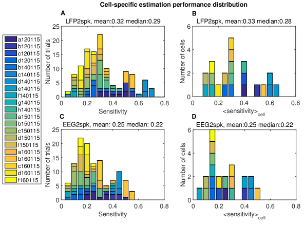
Figure 22: Distribution across trials and cells of spike train estimation performances when using a spike-detection threshold to obtain the same number of spikes in spk_est as in the true spike train (in this case sensitivity and precision of spk_est are equal). (A) Distribution of the sensitivities in the spike train estimation over the trials. (B) Same as (A) when the distribution is across the average sensitivities per cell. (C,D) Same as respectively (A,B) in case of spike estimation from EEG. The legend specifies the cells the data belong to. Mean and median values of the distributions are displayed above each panel. The estimation has been performed by using cell-specific filters and similar results are obtained when using trial-specific and general filters (data not shown).

In figure 22 we show the distribution across trials of the spike train estimation performances performed with cell-specific filters. Analogously to what reported in figure 11, we found that the performances vary broadly from cell to cell but are relatively stable for any given cell. The median values of the sensitivity of the number of estimated spikes within time windows of 26 ms is 0.29$\pm$0.11 (median$\pm$interquartile range/2) for estimation from LFP and 0.22$\pm$0.09 from EEG when using cell-specific filters. Very similar results were obtained also with the trial-specific and general filters. In fact the sensitivity distribution across filters never differed when comparing sensitivity for estimation from LFP and EEG (two-tailed Kolmogorov-Smirnov tests, p>0.45 for LFP and p > 0.21 for EEG).

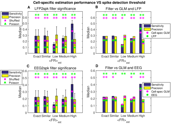
Figure 23: Significance of the spike train cell-specific estimation performance VS spike-detection threshold. We analyze the significance of the Wiener-based estimation and we also compared the performances with the ones obtained by using other two different models that are (i) directly the LFP/EEG and (ii) the GLM to estimate the FR. (A) Spike train estimation performances and their significance as a function of the threshold used to detect the estimated spikes (see section4). To evaluate the significance of the spike estimation, we consider two different null hypotheses (see section 6): (i) the triangles represent the median estimation performances obtained by taking as spk_est a Poisson spike train with the same average FR; (ii) the squares indicate the median estimation performances obtained by randomly placing the estimated spikes in the intervals where the estimated FR was above the spike-detection threshold. The colored bars indicate the median values over the trials, while the error bars represent the interquartile ranges. *$p<10^{-4}$ based on a one-tailed Kolmogorov-Smirnov test comparing the estimation performances against the null hypothesis performances. (B) Comparison with the performances obtained by using other two FR estimation methods as a function of the threshold used to detect the estimated spikes. In particular, we compare the performances given by the FR_est computed as the convolution between the LFP and the (cell-specific) Wiener filter (colored bars) with the ones obtained from taking directly FR_est=LFP (green circles) and by approximating the FR_est through a (cell-specific) GLM (Whittingstall & Logothetis, 2009). *$p<0.03$ based on a one-tailed Kolmogorov-Smirnov test comparing the estimation performances against the null hypothesis performances represented by the LFP (green asterisks) and by the GLM (magenta asterisks). (C,D) Same as respectively (A,B) when the spike estimation is done from the EEG signal; *$p<0.002$ in (C) and *$p<0.03$ in (D). Very similar results are obtained when using trial-specific filters (and trial-specific GLM, data not shown).

In order to evaluate the goodness of the performances obtained, we performed both statistical significance tests and comparisons with the performances obtained by using other methods. We found that the spike train estimation performed with the Wiener kernel is always significant and not only with respect to the chance level (for details see panels (A,C) in figures 23 and 24). Furthermore, when evaluating the performances obtained by taking directly the mass signals as the estimated FR, we found that the Wiener kernel actually produces an enhancement in the spike train estimation performances (p<0.05, according to one-tailed Kolmogorov-Smirnov tests, see panels (B,D) in figures 23 and 24). Therefore, we can conclude that the filtering procedure is effective also after the application of the non-linear threshold to detect spikes.
Finally, we compared the results of our method to those obtained with a general linear model (see section 4) constructed on frequency decomposition of network oscillations which was used in (Whittingstall & Logothetis, 2009) to estimate the firing rate of MUA from both EEG and LFP signals. We estimated the FR by using the GLM and then we applied the spike-detection threshold to estimated spike times (as done in the previous cases). Note that we set the GLM parameters in order to maximize its performances (see figure 5) and we still found that, in all the cases, the performances of the filter were significantly higher (p<0.05, according to one-tailed Kolmogorov-Smirnov tests, see panels (B,D) in figure 23 and panel (B) in figure 24), excepting when estimating spikes from the EEG signal using a general filter (where the performances were not statistically different, see panel (D) in figure 24).
In figures 23 and 24 we report the performances obtained when using cell-specific and general estimation methods, respectively. Importantly, we found that the results were stable across the three kinds of filters we considered. In more detail, we found that the distributions of the performance values associated with the different filters could never be statistically distinguished (respectively p>0.36 (0.21) for estimation from LFP (EEG), according to two-tailed Kolmogorov-Smirnov tests).
We also looked at the spike train estimation performances as a function of the cutoff frequency (in a range between 10 and 90 Hz) of the LFP and of the EEG and we found that the performances monotonically decreased when decreasing the cutoff frequency in a similar way for all estimation considered above (data not shown).

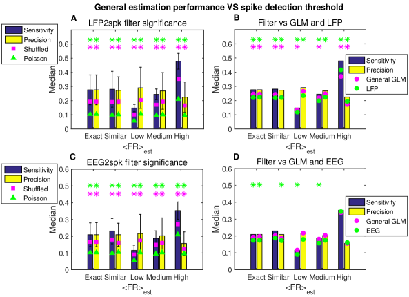
Figure 24: Significance of the spike train general estimation performance VS spike-detection threshold. Same as figure 23 for a general Wiener filter (and a general GLM). (A)*$p<10^{-4}$. (B) *$p<0.05$. (C) *$p<0.03$. (D) *$p<0.05$.

We then investigated how the estimation depends on the spike-detection threshold. We found that, when the estimated FR is exactly equal to the original one, the performances are never distinguishable from those obtained when $\langle FR\rangle_{est}$ was similar to the original one (for details see section 4), for both LFP and EEG cases (p>0.55 according to two-tailed Kolmogorov-Smirnov tests). This means that the performances are robust to a jitter in the spike-detection threshold and that, in particular, we can estimate the spiking activity from mass signals in a blind way, where the only free parameter is given by the range (low, medium or high) of the firing activity. Interestingly, we observed that by augmenting the number of estimated spikes (that is going form the “low” to the “high” $\langle FR\rangle_{est}$), the sensitivity increase is greater than the concurrent precision decrease. This means that, when increasing the number of estimated spikes, the majority of the added spikes will correctly predict true spikes. This fact, together with the already observed positive correlation between average FRs and the synchronization of FR and mass signals (panels (A,B) in figures 15 and 16), suggests that there should be a positive correlation between the spike estimation performances and the average FR. This is indeed what we found, for both LFP and EEG signals (see panels (A,B) in figures 25 and 26).

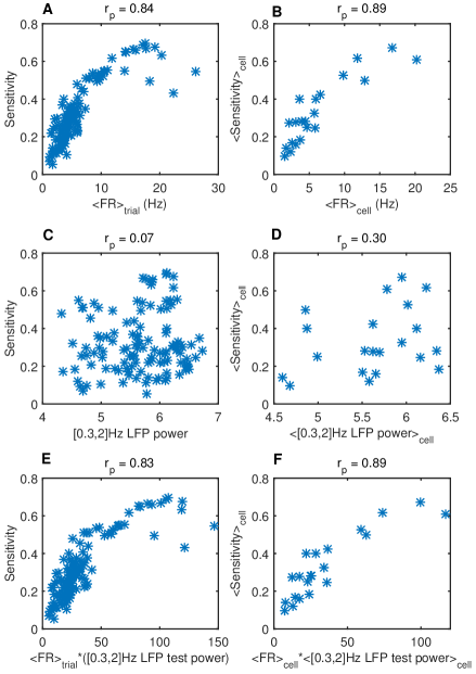
Figure 25: Scatter plots of the performances of the spike trains estimated from LFPs. Spike train estimation performed by using a spike-detection threshold to obtain the same $\langle FR\rangle_{est}$ as in the true spike train (i.e., “exact” case). (A) Sensitivity of the estimated spike train of each trial as a function of the average FR. (C) Sensitivity of the estimated spike train of each trial as a function of the LFP power spectrum in the low delta band, [0.3 2]Hz. (E) Sensitivity of the estimated spike train of each (test) trial as a function of the product between the low LFP power spectrum and the average FR. (B,D,F) Same as respectively (A,C,E) when the data represents the average values over all the trials belonging to a given cell. The values of the Pearson’s correlation between the two plotted variables are reported in the titles of each panel. The showed performances are obtained by using a cell-specific kernel, but similar results are obtained when using both trial-specific and general kernels (data not shown).

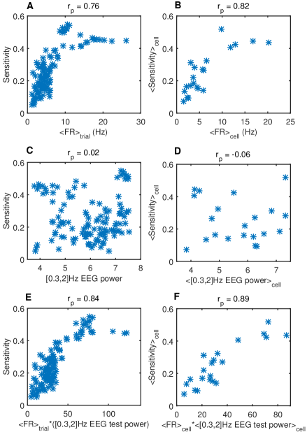
Figure 26: Scatter plots of the performances of the spike trains estimated from EEGs. Same analysis as in figure 25 when estimating the spike trains from EEG signals.

By comparing the scatter plots of the performances of spike train estimation (figures 25 and 26) with the same plots when estimating mass signals (figures 17 and 18), we note that the Pearson’s correlations with the average firing rate increase, while the correlations with the power of the low frequencies decrease steeply. As a result, in both cases, performances correlate the most with the average FRs (whereas, when estimating EEG, the highest correlation was with the EEG low frequency power, see figure 18). This is due to two reasons. First, the positive correlation observed between the (mass signal-FR) synchronization and average FR (see panels (A,B) in figures 15 and 16). Second, when reconstructing the spike train, only the position of the peaks in FR_est matters and not the whole shape of the signal, like in the estimation of analogue (i.e., mass) signals.
When evaluating mass signals, we pointed out that high amplitudes of the low network oscillations facilitated the estimation (see section 18). This is still true, because also in the estimated FR (prior to the spike detection), the frequencies better estimated are the lowest (data not shown). As a results, the correlation between the spike train estimation performances and the product of the average firing rate for the low frequency power is equal (LFP) or higher (EEG; but not lower) to the correlation with the average firing rate alone (see panels (E,F) in figures 25 and 26).

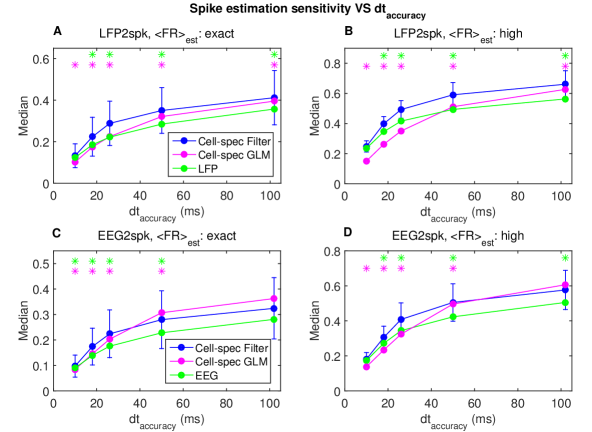
Figure 27: Spike train estimation performance VS dt_accuracy. Median sensitivity of the estimated spike trains as a function of the accuracy used to compare true and estimated spikes (see section 6). (A) The spike-detection threshold is set to obtain the same number of estimated spikes as in the true spike train. Error bars indicates the interquartile range; the models used to evaluate FR_est is specified in the legend. *$p<0.03$ based on a one-tailed Kolmogorov-Smirnov test comparing the estimation performances obtained from the filter against the null hypothesis performances represented by the LFP (green asterisks) and by the GLM (magenta asterisks). (B) Same as (A) when using a spike-detection threshold that results in an high value of $\langle FR\rangle_{est}$ (see section4); *$p<0.005$. (C,D) Same as respectively (A,B) when estimating the spike trains from the EEGs; *$p<0.05$ in (C) and *$p<0.03$ in (D). The showed performances are obtained by using a cell-specific kernel; similar results are obtained when using both trial-specific and general kernels (data not shown).

To conclude the analysis of the spike train estimation, we investigated how the performances vary with the dt_accuracy (in a range between 10 and 102 ms) used to compare estimated and original spike trains (see section 6). In figure 27 we plot the median sensitivity obtained both when using the threshold to obtain the same number of estimated spikes as in the true spike train (panels (A,C)) and the threshold to obtained always an high average firing rate (i.e., 9.4 Hz, see section 4; panels (B,D)). This figure shows that for dt_accuracy$\leq$50 ms, the Wiener filter gives always performances better than the GLM. On the other hand, with the smallest value of dt_accuracy (i.e., 10 ms), the (very low) performance obtained without filtering the mass signals are very close to the one obtained with the filtering procedure and in some cases not significantly lower (p>0.05, according to one-tailed Kolmogorov-Smirnov tests).

Firing rate estimation

We quantified the similarity between original and estimated FRs by means of mutual information. In particular, we computed the information between FR and FR_est after binning the signals in two values which represent respectively a probability of firing equal to zero or higher (for details, see caption figure 28).

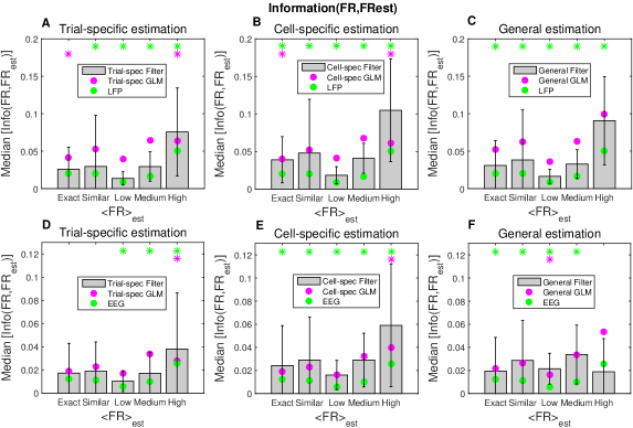
Figure 28: Information between the true and the estimated FR. In order to compute information (see section 1), the original and estimated FRs are firstly smoothed with an Hann window 50ms wide and then their values are binned into two values (0 and 1). For the true FR, all the values above 0 are set to 1, while for the FR_est, the values less or equal to the spike-detection threshold are set to 0 and the ones above to 1. (A) Information between FR and FR_est when using a trial-specific filter as a function of the $\langle FR\rangle_{est}$ class compared with the null hypothesis given by the information obtained from a trial-specific GLM (magenta circles) and by using directly the LFP signal to estimate the FR (green circles). *$p<0.05$ based on one-tailed Kolmogorov-Smirnov tests. (B,C) Same as (A) in case of respectively cell-specific (B) and general (C) estimation. (D-F) Same as (A-B) when the FR estimation is performed from the EEG. We are interested in comparing the level of information across the methods, thus, since the bias is always the same, we do not adopt any bias correction.

Interestingly, we found (see figure 28) that by applying the filter we obtained a more precise estimation of the time intervals when the FR is higher than zero (in addition to the increase of similarity between the position of the peaks in the estimated and true FRs, figures 23 and 24). On the other hand, the comparison with GLM shows that the filter performances are only in few cases better than the GLM ones. This is not surprising, since the GLM is based on the network gamma oscillations, which, during slow wave oscillations, are strongly locked with the firing activity (mainly for the LFP, see panel (C) in figure 5) (Mukovski et al., 2007).

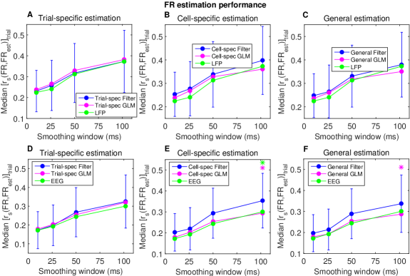
Figure 29: Firing rate estimation performances as a function of the Hann window used to smooth true and estimated FRs. The median value of the Spearman’s correlation between the true and the estimated FR is showed as a function of the Hann window width used to smooth the FRs. The lowest value of smoothing window corresponds to the case where no one smoothing was performed. (A) Estimation performance of the FR obtained from the LFP by using a trial-specific Wiener kernel compared with the null hypothesis represented by the performance obtained from the trial-specific GLM (magenta circles) and by taking as FR_est directly the LFP (green circles). The filter performance are not statistically higher ($p>0.05$, based on one-tailed Kolmogorov-Smirnov tests). (B,C) Same as (A) in case of respectively cell-specific (B) and general (C) estimation. (D-F) Same as (A-B) when the FR estimation is done from the EEG (*$p<0.05$).

We next focused on the FR estimation performances, by analyzing the similarity between the true and the estimated FRs (prior to the use of the spike-detection threshold). Remember that the (true) FR signal is obtained from the spike train and depends on the spike smoothing window chosen that, in our analysis, is 10 ms. After computing FR_est, we convolved both the original and the estimated FRs with an Hann window of a given amplitude and eventually we measured the Spearman’s correlation between the signals. In figure 29, the median correlation is shown as a function of the amplitude of the window used.

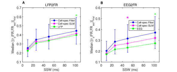
Figure 30: Firing rate estimation performances as a function of the spike smoothing window used to compute the true FR. The median values of the Spearman’s correlation between the true and the estimated FR are showed; error bars represent the interquartile range. Note that, with respect to the analysis showed in figure 29, for each SSW has been computed the relative filters (and GLMs) and no one smoothing has been applied after FR estimation. (A) FR estimated from LFP. (B) FR estimated from EEG. (*$p<0.05$, based on one-tailed Kolmogorov-Smirnov tests). The results are computed from cell-specific filters (similar results are obtained when using trial-specific and general filters; data not shown)

In this analysis we smoothed the FRs after the estimation. However, we obtained similar results also when using from the beginning spike smoothing windows (to compute the original FR, see section 4) of the given amplitudes and then computing the associated filters, without performing a final smoothing (see figure 30). Interestingly, we note that the FR estimation performances obtained with the Wiener filter are not better than the ones obtained respectively without filtering the mass signals and by using the GLM (i.e., $p>0.05$ according to Kolmogorov-Smirnov tests, see figures 29 and 30), whereas, by applying the threshold to detect spikes, the filter’s performances are higher than in the other models (see panels (B,D) in figures 23 and 24). Thus, while the overall shape of estimated FR is very similar over the three models used, the positions of the peak are more close to the original ones when using the Wiener filter to estimate the FR.

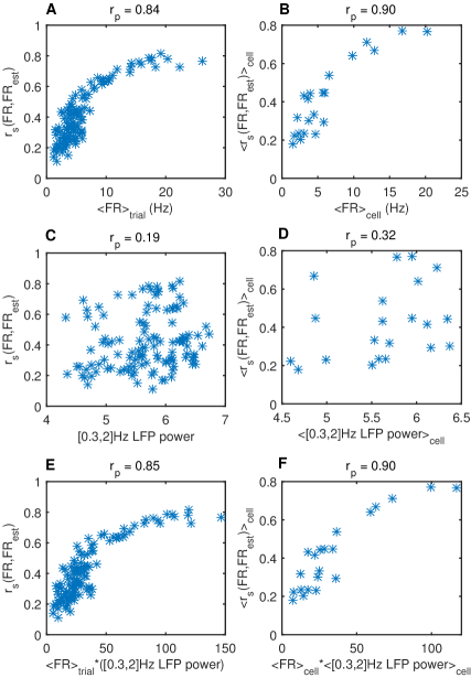
Figure 31: Scatter plots of the performance of the FRs estimated from LFPs. The SSW used to compute the filter is 50 ms wide (very similar results are obtained also when SSW was 10 ms and, after estimation, we smoothed the true and estimated FR with an Hann window of 50 ms, as done in figure 29; data not shown). (A) Performance of the FR estimated from the LFP (as measured by Spearman’s correlation between FR and FR_est) as a function of the average FR (each point represents the values in a trial). (C) FR estimation performance of each trial as a function of the LFP power spectrum in the low delta band, [0.3 2]Hz. (E) FR estimation performance of each trial as a function of the product between the low LFP power spectrum and the average FR. (B,D,F) same as respectively (A,C,E) when each variable is averaged over the trials belonging to a cell. The values of the Pearson’s correlation between the plotted variables are displayed in the panel’s titles. Here we used cell-specific kernels, but similar results are obtained when using both trial-specific and general kernels (data not shown).

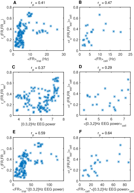
Figure 32: Scatter plots of the performance of the FRs estimated from EEGs. Same analysis performed in figure 31 when estimating the spike trains from EEG signals.

We conclude this section by showing the scatter plots of the FR estimation performances. We already showed the same scatter plots when estimating both the mass signals and the spike trains. In fact they are useful to confirm our observations about the contributions of respectively average firing rates and low frequencies of network oscillations in shaping the relationship between single-unit firing and mass signals. In the FR_est (like in LFP_est and EEG_est) the frequencies better estimated are the lowest (as stated above). Since FRs (unlike spike trains) are analogue signals, as a result there is an increase of the correlations between the FR estimation performances and the low powers of the mass signals with respect to the spike train estimation (see figures 31 and 32). However, we found that the correlation of the performances with the product of average firing rate and low frequency power is respectively equal (LFP) or higher (EEG; but not lower) to the correlation obtained by considering each variable singularly (see panels (E,F) in figures 31 and 32), like in case of spike train estimation.

3 Causality in the estimation

As explained in section 3, the estimations we performed above were acausal. An interesting question is whether there is a dominant direction of causality between spiking and mass activity, or in other words whether the spike times directly caused the mass signal changes or instead the spike times were biased or caused by changes in the mass signal measures. This can be investigated by considering the temporal relationships between signals. Indeed, in the Wiener-Granger spirit (Granger, 1980), one signal may cause the other if its changes consistently anticipate the changes in the other signal (and thus the signal past consistently helps to predict the other signal better than its own past alone). That this may be the case is suggested by the fact that the peaks of the filters are not centered on 0 time lag (and that the filters are not symmetric with respect to the filter peak position). To investigate this issue further, we repeated the analysis (in case of cell-specific and general filters) using both causal and anti-causal filters. The causal filters were obtained by setting to zero the Wiener filters for negative time lags, whereas the anti-causal filters by setting to zero the positive time lag values. Since the acausal filter is the optimal one, the performances will decrease by using other filters. Thus, we quantified the performance reductions to see if and to which extent the causal (or anti-causal) component has a higher weight in the estimation.

In table 1, it is shown the reduction of the performances in case of LFP and EEG estimation. The performance reduction is smaller when the filter is causal, in agreement with the fact that the peaks of the general filters were at positive time lags (see figure 9), indeed the performances obtained with the casual filters are statistically higher than the ones obtained with the anti-causal filters.

	ACAUSAL vs		ACAUSAL vs		CAUSAL >
	CAUSAL		ANTI-CAUSAL		ANTI-CAUSAL
	LFP	EEG	LFP	EEG	LFP	EEG
$r_{s}$	$\delta_{\%}=-9.5$	$\delta_{\%}=-13.7$	$\delta_{\%}=-27.2$	$\delta_{\%}=-18.7$	$p<10^{-10}$	$p=3*10^{-4}$
NMSD	$\delta_{\%}=+6.3$	$\delta_{\%}=+6.2$	$\delta_{\%}=+14.5$	$\delta_{\%}=+9.2$	$p<10^{-10}$	$p=6*10^{-4}$

Table 1: Comparison between the effects of performing causal and anti-causal estimations of mass signals. $\delta_{\%}$ is the median of the relative performance variations observed in each trial with respect to the acausal estimation ($\mathbf{r_{s}}$ is the Spearman’s correlation, and NMSD is the normalized mean squared distance, between the true and the estimate signals). The last two columns display the p-values obtained from a one-tailed Wilcoxon signed rank test comparing the estimation performances obtained by using casual kernels against the performances obtained with anti-causal kernels. We found that the performance reduction is significantly smaller when using casual kernels, both in case of LFP and EEG estimation. Results obtained from cell-specific kernels (but similar dynamics are observed also with a general kernel).

As a control test, we repeated the analysis in the opposite direction, that is when estimating firing activity from the mass signal. We found that, for both firing rate and spike train estimation, larger performances are observed when using an anti-casual filter (see table 2).

	ACAUSAL vs		ACAUSAL vs		CAUSAL >
	CAUSAL		ANTI-CAUSAL		ANTI-CAUSAL
	LFP	EEG	LFP	EEG	LFP	EEG
$r_{s}$	$\delta_{\%}=-17.1$	$\delta_{\%}=-14.2$	$\delta_{\%}=-2.7$	$\delta_{\%}=-8.2$	$p<10^{-10}$	$p=3*10^{-5}$
Sensitivity	$\delta_{\%}=-11.4$	$\delta_{\%}=-6.8$	$\delta_{\%}=-4.7$	$\delta_{\%}=-4.6$	$p=2*10^{-6}$	$p=0.017$

Table 2: Comparison between the effects of performing causal and anti-causal estimations of the firing activity. $\delta_{\%}$ is the median of the relative performance variations observed in each trial with respect to the acausal estimation. $\mathbf{r_{s}}$ is the Spearman’s correlation between $FR$ and $FR_{est}$ and it is evaluated when the SSW was 10 ms; Sensitivity is the sensitivity of the spike times estimation when$\langle FR\rangle_{est}$ is exact (with SSW=10ms) and measured with an accuracy of 26 ms. The last two columns display the p-values obtained from a one-tailed Wilcoxon signed rank test comparing the estimation performances obtained by using anti-casual kernels against the performances obtained from causal kernels. We found that the performance reduction is significantly smaller when using anti-casual kernels, both in case of estimation from LFP and EEG. These data come from cell-specific kernels, but similar dynamics are observed with the general kernels.

Interestingly, the same relationships were observed when estimating the LFP from the spiking activity of pyramidal neurons in deep layers (see section 2), as shown in table 3. This is in agreement with the fact that, also in that case, the peak of the general filter was at a positive time lag (see panel (B) in figure 19).

PYR.	ACAUSAL vs	ACAUSAL vs	CAUSAL >
	CAUSAL	ANTI-CAUSAL	ANTI-CAUSAL
$r_{s}$	$\delta_{\%}=-7.7$	$\delta_{\%}=-42.4$	$p=3*10^{-5}$
NMSD	$\delta_{\%}=+4.1$	$\delta_{\%}=+12.4$	$p=2*10^{-5}$

Table 3: Comparison between the effects of performing causal and anti-causal estimation of LFPs from SUA of excitatory neurons. The spiking activity comes from pyramidal neurons of deep layers (i.e., 5 or 6) and the LFP is recorded at the same depth (3 mice, 7 cells and 23 trials). The table shows the same analysis as in table 1. We found that also with this dataset, when estimating mass signal, the performance reduction is significantly smaller with casual kernels.

Thus, we can conclude that the position of the general filter peak indicates which signal anticipates the other. In particular, in the spk2LFP/EEG estimation, the causal filters work better than the anti-causal, while the opposite is true when estimating the firing activity. Therefore, during slow wave oscillations, the spiking activity (of both inhibitory and excitatory neurons) anticipates and causes mass signals variations, rather than the other way around. This suggests that the types of cells considered here play an important part in the generation of the slow wave cycle captured by the mass signal.

Chapter 4 Conclusions

The motivation of this work was rooted in the following two questions: how can we model the relationship between the single-neuron level and the dynamics observed at the level of population of neurons? How can we study this empirically by analyzing joint recordings?
In section 1 we summarized the results and discussed their implications when the investigation was performed in a modelling framework, while in section 2, we reported the results obtained from the analysis of concomitant LFPs/EEGs and single-unit activity. The implications of these findings, as well as further questions that arise from this work, are reported in the following.

1 Modeling the relationship between the dynamics of single neurons and population of neurons

In chapter 2 we compared in detail the neural population dynamics of recurrent LIF networks when adopting two different models for the synaptic currents at the single-neuron level, namely current-based or conductance-based models. In the former case, the post synaptic potentials of each kind of synapses were constant (see equation 5), while in the conductance-based models, the PSPs depended on the membrane potential of the post synaptic neuron (see equation 6). The comparison of network dynamics was made on networks with all shared parameters set to an equal common value, and with model-specific synaptic parameters set by a novel recursive procedure that makes conductance-based networks (COBN) and current-based networks (CUBN) directly comparable. This means that the differences we found when analyzing the dynamics of population of neurons in the two networks did not depend on the parameter setting, but they were only due to the consequences of adopting a different model at the single-neuron level. Our main result was that, although average firing rates and peak frequency of gamma LFP oscillations in such comparable networks were very similar over a wide range of parameters, other aspects of neural population dynamics (such as shape of oscillation spectra or cross-neuron correlation) were significantly different between CUBN and COBN. In particular, oscillation spectra, gamma synchronization and cross-neuron correlation were more markedly modulated by the external input in COBN than in CUBN. The significance of these findings, and their relationship with both theoretical and experimental literature, is discussed in the following.

1 Establishing comparable networks

The first contribution of the work presented here was to provide a new recursive algorithm to determine the COBN conductance values that correspond to a given set of CUBN synaptic efficacies in networks that have identical values for all the shared parameters. We found that this procedure was able to build two networks displaying relatively small differences, both in the average firing rates and in the gamma frequency peak position, for an input range sufficiently large to encompass both low- and high-conductance states (Destexhe et al., 2003). The relationship of our new procedure with the previous work we built on is discussed in the following.

In a previous work addressing the issue of building equivalent CUBN and COBN models (La Camera et al., 2004), the authors discarded the approach of setting synaptic conductances at fixed average MP (i.e., the one we used in this work) stating that “Although this might work for a single input, it does not work for all inputs in a large pool (results not shown).” La Camera and colleagues proposed instead to build equivalent networks by making both inhibitory and excitatory connectivity free parameters, so that the optimal equivalence was obtained when the CUBN had twice the excitatory and half the inhibitory connectivity of the COBN. Differently from this procedure, in our work all the common parameters of the two networks were identical, including the connectivity matrix. This, in our view, has the advantage that differences in network dynamics can be more directly imputed to changes in model synaptic dynamics. Meffin et al. (2004) determined the value of the conductances starting from a “fixed rough estimate of the average MP” set as the midpoint between threshold and reset potential. The difference with our work is that we used directly the actual average value of the MP of the neurons of each population. Note that there is a discrepancy between the two values since the true average MP was equal or slightly below the reset potential (figure 7D). In extensive initial simulations, we found that using the average MP, rather than the midpoint between threshold and reset potential, made it much easier for the comparable networks to exhibit very close firing rates and gamma spectral peaks (results not shown).

In summary, the comparable networks established with our procedure exhibited average firing rate and position of the peak of the LFP power spectrum that were both similar across network models and were relatively robust to changes in the synaptic reversal potentials. In our view this strengthens the value and usefulness of the setting procedure introduced.

2 Effects of synaptic models on network activity

Previous seminal papers (Meffin et al., 2004; Kuhn et al., 2004; Richardson, 2004) compared the firing rate and MP of conductance- and current-based LIF neurons. Our findings, summarized in table 4, confirmed the main results of these previous works, and extended them in several ways. Our main contribution was to extend the comparison to include other aspects of neural population dynamics. In particular, we considered the effect of the synaptic models on the spectrum of network activity, on the cross-neuron correlations and on the stimulus modulation of these different network features. The significance of these advances is discussed in more detail below.

Correlation dynamics in the networks

Despite the average firing rate was very similar in comparable COBNs and CUBNs, spike trains of different neurons were more correlated in the COBNs than in the CUBNs, with the correlation difference increasing with the external input rate. The fact that the COBN spike train correlation was more strongly modulated by the input rate led to the fact that spike train correlation carried more information in the COBN.

In our networks, the neurons received inputs from the same simulated external pool and this led to values of shared input that were likely higher than those shared by pairs of cortical neurons recorded from different electrodes. However, in the COBN, the dependence of correlation on the network stimuli resembled qualitatively the one observed in real experiments, more than in the CUBN. First, the positive correlation between firing rate intensity and spike train correlation is often observed in neurophysiological experiments, (Kohn & Smith, 2005), and this behavior is only reproduced by the COBN. Further, MP of cortical neurons (Lampl et al., 1999) (but see also (Yu & Ferster, 2010)) are more correlated when they receive an input triggering a stronger response (i.e., having a higher contrast/the correct orientation). This resembles the dynamics displayed here by the COBN, but not by the CUBN. Moreover, in several experiments (Isaacson & Scanziani, 2011) and references therein), the correlation between AMPA and GABA synaptic inputs is stronger the more intense is the stimulus, consistent with the COBN dynamics shown in figure 10A.

The high values of correlation that we found in the COBN might, at first sight, look different from those of Renart et al. (2010) in which a conductance-based LIF network, with a structure similar to the one considered here, displayed a much smaller MP correlation thanks to the decorrelation due to a precise balance between excitation and inhibition. In other words, in that work, AMPA-GABA correlation and cross-neuron MP correlation were described as mutually exclusive. We think that the reason for the difference between their results and those obtained in our work is the crucial assumption of Renart et al. (2010) that AMPA and GABA timescales are identical. In a supplemental analysis the authors showed indeed that, when AMPA synapses were made progressively faster than GABA, the negative feedback was not fast enough to compensate for excitation and hence to decorrelate the neurons; the network became then more synchronized. When in Renart et al. (2010) the authors considered the case in which $\tau_{r-exc}$ = 2 ms and $\tau_{r-inh}$ = 5 ms (very close to our values, see table 1), the correlation between GABA and AMPA currents reached values above 0.5, coherent with our results (figure 10A).

Frequency spectra of network activity

We also compared the frequency spectra of the network activity (as measured by LFP) in COBN and in CUBN. A marked difference was in the larger amount of information and stronger stimulus modulation of the gamma range for COBN. This, in our view, may be explained as follows. When increasing the external input rate, we observed an increase of the cross-neuron spike train correlation in the COBN, which was associated with an increase of the cross-neuron correlation of the synaptic currents (both AMPA and GABA). This caused a stronger modulation of the COBN currents and consequently of the LFP gamma peak. The stronger modulation of the gamma band in turn contributed to the fact that, both when time-constant and time-varying inputs were injected, the COBN carried more information than the CUBN in the gamma band.

Neurophysiological recordings of LFP spectra modulation in visual cortex during stimulation with various kinds of visual stimuli (Henrie & Shapley, 2005; Belitski et al., 2008) reported much broader gamma peaks than the ones we found for COBNs. The width of gamma peaks reported in cortical data was more similar to the broad gamma peak generated by CUBN rather than to the sharp peak generated by the COBN. We hypothesize that the sharpness of the COBN gamma peak may be over-emphasized by the lack of neuron-to-neuron heterogeneity in the specific network models implemented here. Introducing a small degree of variability in neuronal parameters could decrease the correlation in COBN while keeping it stimulus-dependent. An important point for future research is to understand how heterogeneities in network parameters differentially affect COBN and CUBN dynamics.

A final point worth discussing is that the COBN, unlike the CUBN, showed considerable amounts of information about input strength in the LFP power in the frequency range 15– 25 Hz. Notably, the power of real visual cortical LFPs (Belitski et al., 2008) also did not carry information in this frequency range. Belitski and coworkers hypothesized that the 15–25 Hz LFP frequency region related mainly to stimulus-independent neuromodulation. The additive contribution to the LFP of fluctuations generated by a stimulus-unrelated system would potentially cancel out the information generated by the network in this frequency range.

2 Analyzing the relationship between cell-type specific single-unit firing and mass signals

In chapter 3, we investigated the features and the dynamics of the empirical relationship between spiking activity of individual neurons and mass signals. The spiking activity came from both inhibitory and excitatory identified neurons, while the concurrently recorded mass signals was measured as LFPs and EEGs in mice under anesthesia. In particular, we analyzed if and to which extent the spiking activity of single neurons can be estimated in a general and blind way from the mass signals and vice versa. We also characterized (i) how the estimation is significant and if it is robust when increasing the generality of the algorithm used, (ii) which variables mainly affect the relationship between SUAs and mass signals and finally (iii) if there is an empirical causal direction in the relationship.

1 Stability of the relationship

We showed that, during slow wave oscillations, we can estimate in a general way the slow oscillations of mass signals from the spiking activity of a single neuron, both inhibitory (fast-spiking) and excitatory. More precisely, we estimated with a strong accuracy the LFP (median Spearman’s correlation, $\langle r_{s}\rangle$, around 0.6) and, with a good accuracy, even the EEG ($\langle r_{s}\rangle$ around 0.5) from the spiking activity of fast-spiking interneurons in layer 2. Similar results were obtained also when estimating the LFP from the spiking activity of a pyramidal neuron ($\langle r_{s}\rangle$ around 0.5) in deep layers. On the other hand, we were able to estimate (with a precision of 26 ms) in median the 30% of the spike times (mainly depending on the average firing rate) of a single fast-spiking neuron from the mass signals recorded (i.e., LFPs and EEGs). The estimations were performed with a simple linear model to which we added a non-linear threshold in order to detect spike times. We found that, in both directions, the estimations were highly significant. In particular, in case of spike train estimation, the spikes were not simply placed at chance level where the estimated FR was high (i.e., above thresholds), but the positions of the peaks were actually related to the spike times. We also verified that the filtering procedure was really useful to increase the performances and we finally made a comparison with the general linear model used in (Whittingstall & Logothetis, 2009), founding that the Wiener filter gave very similar results when estimating FR, but higher performances when evaluating spike times.
Furthermore the results of all the estimations performed were remarkably stable across cells and animals, allowing a truly general estimation with no reduction in the performances.

The relationship between mass signals and the underlying spiking activity has been investigated widely using spike-triggered average and more complex techniques during both sensory stimulation and absence of stimulus (Schwartz et al., 2006; Rasch et al., 2008, 2009; Nauhaus et al., 2009; Okun et al., 2010; Zanos et al., 2012; Hall et al., 2014; Whittingstall & Logothetis, 2009). In particular, Rasch et al. (2009) used animal-specific Wiener filters to estimate the firing rate of MUAs from LFPs and Hall et al. (2014) applied a similar method to estimate LFPs from the SUAs of multiple (not specified) neurons. The same groups performed also the linear estimation in the opposite direction, by computing the firing rate (Hall et al., 2014) and the spike times (Rasch et al., 2008) from the LFP. Whittingstall & Logothetis (2009) used general linear models based on frequency decomposition of EEG (and LFP) to reconstruct the firing rate of MUAs. However, to our knowledge, this is the first case in which this estimation has been performed from the activity of an individual (genetically-identified) GABAergic interneuron and by using the same filter across all the animals to estimate mass signals.
Note that LFPs integrate the postsynaptic signals coming from hundreds to thousands of neurons (Logothetis, 2003), and EEG integrates signals on even a wider area than LFP. On the other hand, the activity of a single neuron is a more localized signal than the multi-unit activity, which has been used in the majority of the above mentioned works. Furthermore the interneurons, due to their geometrical arrangement, are likely to generate small dipoles (compared with pyramidal neurons) when active (Murakami & Okada, 2006). For these reasons, the strong and robust relationship found between mass signals and single-unit spike trains is not trivially expected a priori. It reflects the strong synchronization in the cortex activity observed during slow wave oscillations, which is able to recruit also the interneuron activity suggesting the existence of a robust control mechanism of interneurons on network dynamics.
We found a very strong coupling even between the firing activity of single pyramidal neurons and LFP, indeed, in presence of a strong reduction in the average firing rates (median of 1.7 Hz, while it was 4.5 Hz for fast-spiking neurons), which is a fundamental variable when performing a linear reconstruction, the estimation performances decrease only slightly . This is not surprising since the majority of the works that investigated the relationship between LFPs/EEGs and firing activity considered actually the firing activity of pyramidal neurons (see section 1).

2 Variables shaping the relationship

The estimation performances varied a lot from trial to trial (being relatively constant for trials of the same cell) overall resulting in a wide range of values. Our purpose is both to understand how the mass signals time courses relate to the underlying spiking activity of single neurons and to develop a general blind toolbox to estimate the EEGs and the LFPs from SUAs and vice versa, with known estimation accuracy. These questions are of paramount importance (i) to understand how mass signals rely on the underlying neural computation, (ii) to understand how the firing of single cells relates to the circuit “context” which led the neuron to fire (iii) and also for neuroprosthetic applications.
To achieve these goals, we investigated more in detail how the performances of each trial are determined. In particular, we analyzed the correlation properties of the performances with different features of both mass signals and spiking activity.
We found that the variables mainly shaping the estimation performances are the average firing rate and the power of the low frequencies of the mass signals. Both of them are positively correlated with the performances (and the highest correlation is usually observed with the product of average firing rate and power spectrum), but their relative weight depends on the estimation performed.
When estimating continuous signals (i.e., LFPs, EEGs and FRs), the relative contributions of average firing rate and low power of the LFP or EEG depend on the synchronization between the firing activity and the mass signals. If the firing activity is synchronized with the mass signals (as in the LFP case), when increasing the average firing rate the performances strongly increase, because we have more spikes to reconstruct the signals and in the “right” places. On the other hand, when investigating the relationship between EEGs and SUAs, the synchronization between FRs and mass signals is lower and the weight of low frequencies power in determining the performances increases. This is due to the fact that the slowest oscillations are the strongest, therefore the ones better estimated with a linear method (in agreement with previous results Rasch et al., 2009; Hall et al., 2014). The more low frequencies we have, the higher the performances will be (while a high number of spikes is not useful, since the spikes could be no synchronized with the EEG signal).
When estimating spike trains, instead, the performance shows always the largest correlation with the average firing rate (for estimation from both LFPs and EEGs). In that case, indeed, we only take into account the positions of the peaks in the estimated FR and (even due to the increase of synchronization between mass signals and firing rate when increasing the average firing rate) the more spikes there are, the more likely the FR_est peaks will be close to the original ones. On the other hand, when the firing activity is too sparse, a threshold applied on a linearly estimated signal cannot efficiently detect the spike times.

3 Causality in the relationship

An important and open issue in the comprehension of the interactions occurring between single-cell dynamics and the dynamics of mesoscopic and macroscopic circuits of neurons is given by the causality in the relationship between these two levels of investigation. The LFP is mostly generated by the totality of synaptic input and local processing in a region (Rasch et al., 2008), however, the way it is related to the spiking output of underlying neurons is unknown. In other words: mass signals, such as LFPs and EEGs, can be considered as the “input” for the network spiking dynamics, being thus responsible for the underlying single-neuron activity, or vice versa the collective single-neuron activities causally shape the time course of the mass signals? Probably no one of these two extreme cases describes the truth, since the neural circuits in the cerebral cortex are characterized by recurrent connections, complex patterns of excitation and inhibition and inputs from multiple structures (Douglas et al., 1989; Douglas & Martin, 2004). Thus we did not assume any a-priori causal constraint in the investigation of the relationship between SUAs and mass signals and our estimation were not causal (indeed the filters were not equal to zero for negative time lags). This means that we could use spikes fired in $t>t^{*}$ to estimate mass signals in $t^{*}$and vice versa.

To have a deeper insight about the causality issue, we tested if and to which extent the performances are affected when imposing a causal direction in the relation between SUAs and mass signals. We cross-validated the results by repeated the analysis on both the directions of estimation (i.e., spk2LFP/EEG and LFP/EEG2spk) and we found concordant results. In particular, when assuming that the single-neuron spiking activity causally shapes the mass signal fluctuations, the estimation performances were less affected with respect to imposing an anti-causal relation (analogously to what found by Rasch et al. (2009) when estimating the LFPs from MUAs during visual stimulation). This was observed for both interneuron in layer 2 and pyramidal neurons in deep layers.
In conclusion, we found that spike times anticipate changes in the time course of mass signals in a reliable way (and vice versa), thus, from an empirical point of view, the spiking activity of single neurons can be viewed as a “stimulus” for the mass signals. This result is not obvious and requires further investigations, indeed the spiking activity is usually considered as the output of a cortical area, whereas the LFP as the processing of the entire subthreshold local signals (Logothetis, 2008).

3 Perspectives

In chapter 2, we investigated the effects of assuming different single-neuron models on network dynamics as a function of the input to the network. In that network model there were two sources of noise. The first was due to the stochastic process, which affected the time varying rates, $\nu_{ext}(t)$, identical for all neurons. The second source of noise, instead, was due to the fact that each neuron received an independent realization of the Poisson process with rate $\nu_{ext}(t)$. The fluctuations due to this second source of noise were uncorrelated across neurons and, in particular, they increased with the input rate.
However, noise in the brain is correlated across neurons, meaning the fluctuations in the response of a neuron at fixed stimulus are correlated with the fluctuations of other neurons (Averbeck et al., 2006). If assuming the noise is uncorrelated, the investigation of network dynamics is simpler and population coding is relatively well understood (Averbeck et al., 2006). Therefore, for the computational work, it is important to extend the theories to take into account noise correlation and, in particular, to investigate how correlated noise affect network dynamics. Thus, a direction of further investigation would be to disentangle the role of changes in the mean input rate (that is a source of correlated noise) from the ones of changes in the variance of the input across neurons (that is a source of uncorrelated noise) in shaping network dynamics.
Another very interesting direction for further research consists on the the analysis of network dynamics when changing the topology of the network (Prettejohn et al., 2011). In our view, it would be worth investigating for example, the effect of changing synaptic dynamics and other biophysical parameters in networks composed of clusters of strongly interconnected neurons (Litwin-Kumar & Doiron, 2012) and compare it with the dynamics generated by the random connectivity that we adopted. Studies like this would help to understand the relationship between the anatomical pattern of synaptic connections and the pattern of functional connectivity (defined as the set of statistical dependencies between the activity of the elements of the neural network). This is a hot topic in neuroscience (Fasoli et al., 2015; Deco et al., 2013; Cabral et al., 2012; Eickhoff et al., 2010; Ponten et al., 2010; Sporns et al., 2004)

In the work described in chapter 3, we focused on the relationship between single-neuron activity and mesoscopic or macroscopic signals, as measured respectively by LFPs or EEGs. We found that the relationships of SUAs with respectively LFPs and EEGs have some similarities (for example, the shapes of the filters, the estimation robustness when using more general filters, the empirical causal direction of the relationships etc…). This is not surprising, indeed, the LFPs are considered as the building blocks of EEG signals (da Silva, 2013) or, analogously, a more localized variant of the EEGs (Whittingstall & Logothetis, 2009). Nevertheless this represents a first approximation of the relationship occurring between LFPs and EEGs. In order to gain a better insight about this relation, we could take advantage of the fact that in our datasets SUA, LFP and EEG are simultaneously recorded. Thus, we could investigate more in detail which aspects of the relationship between SUA and LFP differs from the one existing between SUA and EEG. In particular, we could identify which dynamics in the relationship between EEGs and SUAs are less reliable (with respect to the LFP-SUA case), for example, by performing frequency decomposition of the mass signals and studying the locking of SUAs with phase and power of network oscillations. In the end, the next purpose will be to investigate the relationship between LFPs and EEGs by pointing out the dynamics responsible for the performance decrease observed when estimating single-neuron FR from EEG (and vice versa).

Acknowledgements

First and foremost, my deepest gratitude goes to my Ph.D. supervisor Professor Stefano Panzeri, which gave me the opportunity to enter the fascinating field of neuroscience.

I wish to thank Alberto Mazzoni and Daniel Chicharro for many valuable suggestions and (not only scientific) discussions, for sharing thoughts and support during these years… it was really a pleasure to share the office with you! I cannot avoid to mention Rupan Raventos, which has been an example of consistency for all of us.

A special thank to Pietro Salvagnini for his friendship and for being always available to help me and to answer my questions. I am also grateful to Cesare Magri for a first version of the code I used to perform my work.

I am not forgetting Stefano Zucca, Tommaso Fellin and other colleagues in the laboratory of Tommaso Fellin, which kindly provided me with the data for the analysis performed in this thesis.

I want to thank Alessandro Maccione for his motivating words when I really needed them and Paolo Mereghetti, which has been my last office mate at IIT… before the “diaspora”.

Thanks to my family which stood by me in all the good and bad moments. I simply would not be here without their love and dedication…

Finally, thanks to my wife, Elisabetta, which was surprisingly able to give me unexpected wonderful times in everyday life… you have been my constant source of energy and motivation.

PS: è stato divertente giocare in allegria,
c’è un solo inconveniente che il tempo vola via…
Addio addio amici addio.

References

- (1)
- Abeles (1991) Abeles, M. (1991), Corticonics: Neural circuits of the cerebral cortex, Cambridge University Press.
- Averbeck et al. (2006) Averbeck, B. B., Latham, P. E. & Pouget, A. (2006), ‘Neural correlations, population coding and computation’, Nat Rev Neurosci 7(5), 358–66.
- Babadi & Abbott (2010) Babadi, B. & Abbott, L. F. (2010), ‘Intrinsic stability of temporally shifted spike-timing dependent plasticity’, PLoS computational biology 6(11), e1000961.
- Bansal et al. (2011) Bansal, A. K., Vargas-Irwin, C. E., Truccolo, W. & Donoghue, J. P. (2011), ‘Relationships among low-frequency local field potentials, spiking activity, and three-dimensional reach and grasp kinematics in primary motor and ventral premotor cortices’, Journal of neurophysiology 105(4), 1603–1619.
- Bear et al. (2007) Bear, M., Connors, B. & Paradiso, M. (2007), Neuroscience exploring the brain, third edn, Lippincott Williams & Wilkins.
- Belitski et al. (2008) Belitski, A., Gretton, A., Magri, C., Murayama, Y., Montemurro, M. A., Logothetis, N. K. & Panzeri, S. (2008), ‘Low-frequency local field potentials and spikes in primary visual cortex convey independent visual information’, J Neurosci 28(22), 5696–709.
- Berens (2009) Berens, P. (2009), ‘Circstat: A matlab toolbox for circular statistics’, Journal of Statistical Software 31(10), 1–21.
- Berens et al. (2010) Berens, P., Logothetis, N. K. & Tolias, A. S. (2010), ‘Local field potentials, bold and spiking activity-relationships and physiological mechanisms’, Nature Precedings pp. 1–27.
- Braitenberg & Schüz (1991) Braitenberg, V. & Schüz, A. (1991), Anatomy of the cortex : statistics and geometry, Studies of brain function, Springer-Verlag, Berlin ; New York.
- Brunel (2013) Brunel, N. (2013), Dynamics of Neural Networks, CRC Press, Boca Raton, chapter 25, pp. 489–512.
- Brunel & Wang (2003) Brunel, N. & Wang, X.-J. (2003), ‘What determines the frequency of fast network oscillations with irregular neural discharges?’, J. Neurophysiol. 90, 415–430.
- Buzsaki et al. (2012) Buzsaki, G., Anastassiou, C. A. & Koch, C. (2012), ‘The origin of extracellular fields and currents–eeg, ecog, lfp and spikes’, Nat Rev Neurosci 13(6), 407–20.
- Cabral et al. (2012) Cabral, J., Hugues, E., Kringelbach, M. L. & Deco, G. (2012), ‘Modeling the outcome of structural disconnection on resting-state functional connectivity’, Neuroimage 62(3), 1342–1353.
- Canolty et al. (2010) Canolty, R. T., Ganguly, K., Kennerley, S. W., Cadieu, C. F., Koepsell, K., Wallis, J. D. & Carmena, J. M. (2010), ‘Oscillatory phase coupling coordinates anatomically dispersed functional cell assemblies’, Proceedings of the National Academy of Sciences 107(40), 17356–17361.
- Cauli et al. (2000) Cauli, B., Porter, J. T., Tsuzuki, K., Lambolez, B., Rossier, J., Quenet, B. & Audinat, E. (2000), ‘Classification of fusiform neocortical interneurons based on unsupervised clustering’, Proceedings of the National Academy of Sciences 97(11), 6144–6149.
-
Cavallari et al. (2014)
Cavallari, S., Panzeri, S. & Mazzoni, A. (2014), ‘Comparison of the dynamics of neural interactions
between current-based and conductance-based integrate-and-fire recurrent
networks’, Frontiers in neural circuits 8.
http://www.ncbi.nlm.nih.gov/pmc/articles/PMC3943173/ - Chandrasekaran et al. (2010) Chandrasekaran, C., Turesson, H. K., Brown, C. H. & Ghazanfar, A. A. (2010), ‘The influence of natural scene dynamics on auditory cortical activity’, Journal of Neuroscience 30(42), 13919–13931.
- Cheng-yu et al. (2009) Cheng-yu, T. L., Poo, M.-m. & Dan, Y. (2009), ‘Burst spiking of a single cortical neuron modifies global brain state’, Science 324(5927), 643–646.
- Contreras (2004) Contreras, D. (2004), ‘Electrophysiological classes of neocortical neurons’, Neural Networks 17(5), 633–646.
- Crumiller et al. (2011) Crumiller, M., Knight, B., Yu, Y. & Kaplan, E. (2011), ‘Estimating the amount of information conveyed by a population of neurons’, Frontiers in neuroscience 5.
- da Silva (2013) da Silva, F. L. (2013), ‘Eeg and meg: relevance to neuroscience’, Neuron 80(5), 1112–1128.
- Dayan & Abbott (2001) Dayan, P. & Abbott, L. (2001), Theoretical neuroscience, MIT press.
- De La Rocha et al. (2007) De La Rocha, J., Doiron, B., Shea-Brown, E., Josić, K. & Reyes, A. (2007), ‘Correlation between neural spike trains increases with firing rate’, Nature 448(7155), 802–806.
- de Ruyter van Steveninck et al. (1997) de Ruyter van Steveninck, R., Lewen, G., Strong, S., Koberle, R. & Bialek, W. (1997), ‘Reproducibility and variability in neural spike trains’, Science 275, 1805–1808.
- Deco et al. (2008) Deco, G., Jirsa, V. K., Robinson, P. A., Breakspear, M. & Friston, K. (2008), ‘The dynamic brain: from spiking neurons to neural masses and cortical fields’, PLoS Comput Biol 4(8), e1000092.
- Deco et al. (2013) Deco, G., Ponce-Alvarez, A., Mantini, D., Romani, G. L., Hagmann, P. & Corbetta, M. (2013), ‘Resting-state functional connectivity emerges from structurally and dynamically shaped slow linear fluctuations’, The Journal of Neuroscience 33(27), 11239–11252.
- Destexhe & Pare (1999) Destexhe, A. & Pare, D. (1999), ‘Impact of network activity on the integrative properties of neocortical pyramidal neurons in vivo’, J Neurophysiol 81(4), 1531–47.
- Destexhe et al. (2001) Destexhe, A., Rudolph, M., Fellous, J.-M. & Sejnowski, T. J. (2001), ‘Fluctuating synaptic conductances recreate in vivo-like activity in neocortical neurons’, Neuroscience 107(1), 13–24.
- Destexhe et al. (2003) Destexhe, A., Rudolph, M. & Pare, D. (2003), ‘The high-conductance state of neocortical neurons in vivo’, Nat Rev Neurosci 4(9), 739–51.
- Douglas & Martin (2004) Douglas, R. J. & Martin, K. A. (2004), ‘Neuronal circuits of the neocortex’, Annu. Rev. Neurosci. 27, 419–451.
- Douglas et al. (1989) Douglas, R. J., Martin, K. A. & Whitteridge, D. (1989), ‘A canonical microcircuit for neocortex’, Neural computation 1(4), 480–488.
- Ecker et al. (2010) Ecker, A. S., Berens, P., Keliris, G. A., Bethge, M., Logothetis, N. K. & Tolias, A. S. (2010), ‘Decorrelated neuronal firing in cortical microcircuits’, Science 327(5965), 584–7.
- Eickhoff et al. (2010) Eickhoff, S. B., Jbabdi, S., Caspers, S., Laird, A. R., Fox, P. T., Zilles, K. & Behrens, T. E. (2010), ‘Anatomical and functional connectivity of cytoarchitectonic areas within the human parietal operculum’, The Journal of neuroscience 30(18), 6409–6421.
- Einevoll et al. (2013) Einevoll, G. T., Kayser, C., Logothetis, N. K. & Panzeri, S. (2013), ‘Modelling and analysis of local field potentials for studying the function of cortical circuits’, Nature Reviews Neuroscience 14, 770–785.
-
Fasoli et al. (2015)
Fasoli, D., Faugeras, O. & Panzeri, S. (2015), ‘A formalism for evaluating analytically the
cross-correlation structure of a firing-rate network model’, The Journal
of Mathematical Neuroscience (JMN) 5(1).
http://dx.doi.org/10.1186/s13408-015-0020-y - Gabbiani & Koch (1998) Gabbiani, F. & Koch, C. (1998), ‘Principles of spike train analysis’, Methods in neuronal modeling 12(4), 313–360.
- Gerstner et al. (2014) Gerstner, W., Kistler, W. M., Naud, R. & Paninski, L. (2014), Neuronal dynamics: from single neurons to networks and models of cognition, Cambridge University Press.
- Gieselmann & Thiele (2008) Gieselmann, M. & Thiele, A. (2008), ‘Comparison of spatial integration and surround suppression characteristics in spiking activity and the local field potential in macaque v1’, European Journal of Neuroscience 28, 447–459.
- Gillespie (1996) Gillespie, D. T. (1996), ‘Exact numerical simulation of the ornstein-uhlenbeck process and its integral’, Phys Rev E Stat Phys Plasmas Fluids Relat Interdiscip Topics 54(2), 2084–2091.
- Grabska-Barwińska & Latham (2014) Grabska-Barwińska, A. & Latham, P. E. (2014), ‘How well do mean field theories of spiking quadratic-integrate-and-fire networks work in realistic parameter regimes?’, Journal of computational neuroscience 36(3), 469–481.
- Granger (1980) Granger, C. W. (1980), ‘Testing for causality: a personal viewpoint’, Journal of Economic Dynamics and control 2, 329–352.
- Gross et al. (2013) Gross, J., Hoogenboom, N., Thut, G., Schyns, P., Panzeri, S., Belin, P. & Garrod, S. (2013), ‘Speech rhythms and multiplexed oscillatory sensory coding in the human brain’, PLoS Biol 11(12), e1001752.
- Gutig et al. (2013) Gutig, R., Gollisch, T., Sompolinsky, H. & Meister, M. (2013), ‘Computing complex visual features with retinal spike times’, PLoS One 8(1), e53063.
- Hall et al. (2014) Hall, T. M., Nazarpour, K. & Jackson, A. (2014), ‘Real-time estimation and biofeedback of single-neuron firing rates using local field potentials’, Nature communications 5.
- Harris & Thiele (2011) Harris, K. D. & Thiele, A. (2011), ‘Cortical state and attention’, Nature reviews neuroscience 12(9), 509–523.
- Helias et al. (2010) Helias, M., Deger, M., Rotter, S. & Diesmann, M. (2010), ‘Instantaneous non-linear processing by pulse-coupled threshold units’, PLoS computational biology 6(9), e1000929.
- Henrie & Shapley (2005) Henrie, J. A. & Shapley, R. (2005), ‘Lfp power spectra in v1 cortex: the graded effect of stimulus contrast’, J Neurophysiol 94(1), 479–90.
- Holmgren et al. (2003) Holmgren, C., Harkany, T., Svennenfors, B. & Zilberter, Y. (2003), ‘Pyramidal cell communication within local networks in layer 2/3 of rat neocortex’, The Journal of physiology 551(1), 139–153.
- Houweling & Brecht (2008) Houweling, A. R. & Brecht, M. (2008), ‘Behavioural report of single neuron stimulation in somatosensory cortex’, Nature 451(7174), 65–68.
- Hubel & Wiesel (1959) Hubel, D. H. & Wiesel, T. N. (1959), ‘Receptive fields of single neurones in the cat’s striate cortex’, The Journal of physiology 148(3), 574–591.
- Hubel & Wiesel (1962) Hubel, D. H. & Wiesel, T. N. (1962), ‘Receptive fields, binocular interaction and functional architecture in the cat’s visual cortex’, The Journal of physiology 160(1), 106–154.
- Hubel & Wiesel (1968) Hubel, D. H. & Wiesel, T. N. (1968), ‘Receptive fields and functional architecture of monkey striate cortex’, The Journal of physiology 195(1), 215–243.
- Isaacson & Scanziani (2011) Isaacson, J. S. & Scanziani, M. (2011), ‘How inhibition shapes cortical activity’, Neuron 72(2), 231–43.
- Izhikevich (2007) Izhikevich, E. M. (2007), Dynamical systems in neuroscience, MIT press.
- Johnston & Wu (1995) Johnston, D. & Wu, S. (1995), Foundations of cellular neurophysiology, MIT press, Cambridge, MA.
- Kandel et al. (1999) Kandel, E., Schwartz, J. & Jessel, T. (1999), Fondamenti delle neuroscienze e del comportamento, first italian edn, Casa Editrice Ambrosiana.
- Kayser et al. (2009) Kayser, C., Montemurro, M., Logothetis, N. & Panzeri, S. (2009), ‘Spike-phase coding boosts and stabilizes information carried by spatial and temporal spike patterns’, Neuron 61(4), 597–608.
- Koch (1999) Koch, C. (1999), Biophysics of computation : information processing in single neurons, Computational neuroscience, Oxford University Press, New York.
- Koch (2004) Koch, C. (2004), Biophysics of computation: information processing in single neurons, Oxford University Press.
- Kohn & Smith (2005) Kohn, A. & Smith, M. A. (2005), ‘Stimulus dependence of neuronal correlation in primary visual cortex of the macaque’, J Neurosci 25(14), 3661–73.
- Kuhn et al. (2004) Kuhn, A., Aertsen, A. & Rotter, S. (2004), ‘Neuronal integration of synaptic input in the fluctuation-driven regime’, J Neurosci 24(10), 2345–56.
- Kumar et al. (2008) Kumar, A., Schrader, S., Aertsen, A. & Rotter, S. (2008), ‘The high-conductance state of cortical networks’, Neural Comput 20(1), 1–43.
- La Camera et al. (2004) La Camera, G., Senn, W. & Fusi, S. (2004), ‘Comparison between networks of conductance-and current-driven neurons: stationary spike rates and subthreshold depolarization’, Neurocomputing 58, 253–258.
- Lampl et al. (1999) Lampl, I., Reichova, I. & Ferster, D. (1999), ‘Synchronous membrane potential fluctuations in neurons of the cat visual cortex’, Neuron 22(2), 361–74.
- Lapicque (1907) Lapicque, L. (1907), ‘Recherches quantitatives sur l’excitation electrique des nerfs traitee comme une polarization’, Journal de Physiologie et Pathologie Général 9, 620–635.
- Lim & Goldman (2013) Lim, S. & Goldman, M. S. (2013), ‘Balanced cortical microcircuitry for maintaining information in working memory’, Nat Neurosci 16(9), 1306–14.
- Linden et al. (2011) Linden, H., Tetzlaff, T., Potjans, T. C., Pettersen, K. H., Grun, S., Diesmann, M. & Einevoll, G. T. (2011), ‘Modeling the spatial reach of the lfp’, Neuron 72(5), 859–72.
- Litwin-Kumar & Doiron (2012) Litwin-Kumar, A. & Doiron, B. (2012), ‘Slow dynamics and high variability in balanced cortical networks with clustered connections’, Nature neuroscience 15(11), 1498–1505.
- Logothetis (2002) Logothetis, N. K. (2002), ‘The neural basis of the blood–oxygen–level–dependent functional magnetic resonance imaging signal’, Philosophical Transactions of the Royal Society B: Biological Sciences 357(1424), 1003–1037.
- Logothetis (2003) Logothetis, N. K. (2003), ‘The underpinnings of the bold functional magnetic resonance imaging signal’, J. Neurosci. 23, 3963–3971.
- Logothetis (2008) Logothetis, N. K. (2008), ‘What we can do and what we cannot do with fMRI’, Nature 12, 869–878.
- Logothetis et al. (2012) Logothetis, N. K., Eschenko, O., Murayama, Y., Augath, M., Steudel, T., Evrard, H., Besserve, M. & Oeltermann, A. (2012), ‘Hippocampal-cortical interaction during periods of subcortical silence’, Nature 491(7425), 547–553.
- Logothetis et al. (2007) Logothetis, N., Kayser, C. & Oeltermann, A. (2007), ‘In vivo measurement of cortical impedance spectrum in monkeys: implications for signal propagation’, Neuron 55, 809–823.
- Lorente de NO (1947) Lorente de NO, R. (1947), ‘Action potential of the motoneurons of the hypoglossus nucleus’, J Cell Physiol 29(3), 207–87.
- Luo & Poeppel (2007) Luo, H. & Poeppel, D. (2007), ‘Phase patterns of neural responses reliably discriminate speech in human auditory cortex’, Neuron 54, 1001–1010.
- Magri et al. (2009) Magri, C., Whittingstall, K., Singh, V., Logothetis, N. K. & Panzeri, S. (2009), ‘A toolbox for the fast information analysis of multiple-site lfp, eeg and spike train recordings’, BMC neuroscience 10(1), 81.
- Maimon & Assad (2009) Maimon, G. & Assad, J. A. (2009), ‘Beyond poisson: increased spike-time regularity across primate parietal cortex’, Neuron 62(3), 426–40.
- Mazzoni et al. (2011) Mazzoni, A., Brunel, N., Cavallari, S., Logothetis, N. K. & Panzeri, S. (2011), ‘Cortical dynamics during naturalistic sensory stimulations: experiments and models’, J Physiology Paris 105(1-3), 2–15.
- Mazzoni et al. (2008) Mazzoni, A., Panzeri, S., Logothetis, N. K. & Brunel, N. (2008), ‘Encoding of naturalistic stimuli by local field potential spectra in networks of excitatory and inhibitory neurons’, PLoS Computational Biology 4(12), e1000239.
- Mazzoni et al. (2010) Mazzoni, A., Whittingstall, K., Brunel, N., Logothetis, N. & Panzeri, S. (2010), ‘Understanding the relationships between spike rate and delta/gamma frequency bands of lfps and eegs using a local cortical network model’, Neuroimage 52, 956–972.
- Meffin et al. (2004) Meffin, H., Burkitt, A. N. & Grayden, D. B. (2004), ‘An analytical model for the "large, fluctuating synaptic conductance state" typical of neocortical neurons in vivo’, J Comput Neurosci 16(2), 159–75.
- Memmesheimer (2010) Memmesheimer, R.-M. (2010), ‘Quantitative prediction of intermittent high-frequency oscillations in neural networks with supralinear dendritic interactions’, Proceedings of the National Academy of Sciences 107(24), 11092–11097.
- Mitzdorf (1985) Mitzdorf, U. (1985), ‘Current source-density method and application in cat cerebral cortex: investigation of evoked potentials and eeg phenomena’, Physiol Rev 65, 37–100.
- Mongillo et al. (2012) Mongillo, G., Hansel, D. & van Vreeswijk, C. (2012), ‘Bistability and spatiotemporal irregularity in neuronal networks with nonlinear synaptic transmission’, Physical review letters 108(15), 158101.
- Montemurro et al. (2008) Montemurro, M. A., Rasch, M. J., Murayama, Y., Logothetis, N. K. & Panzeri, S. (2008), ‘Phase-of-firing coding of natural visual stimuli in primary visual cortex’, Current Biology 18, 375–380.
- Mormann et al. (2000) Mormann, F., Lehnertz, K., David, P. & Elger, C. E. (2000), ‘Mean phase coherence as a measure for phase synchronization and its application to the eeg of epilepsy patients’, Physica D: Nonlinear Phenomena 144(3), 358–369.
- Mountcastle (1978) Mountcastle, V. (1978), ‘An organizing principle for cerebral function: the unit model and the distributed system’.
- Mountcastle (1957) Mountcastle, V. B. (1957), ‘Modality and topographic properties of single neurons of cat’s somatic sensory cortex’, J neurophysiol 20(4), 408–434.
- Mukovski et al. (2007) Mukovski, M., Chauvette, S., Timofeev, I. & Volgushev, M. (2007), ‘Detection of active and silent states in neocortical neurons from the field potential signal during slow-wave sleep’, Cerebral Cortex 17(2), 400–414.
- Murakami & Okada (2006) Murakami, S. & Okada, Y. (2006), ‘Contributions of principal neocortical neurons to magnetoencephalography and electroencephalography signals’, The Journal of physiology 575(3), 925–936.
- Musall et al. (2014) Musall, S., von Pföstl, V., Rauch, A., Logothetis, N. K. & Whittingstall, K. (2014), ‘Effects of neural synchrony on surface eeg’, Cerebral Cortex 24(4), 1045–1053.
- Nauhaus et al. (2009) Nauhaus, I., Busse, L., Carandini, M. & Ringach, D. L. (2009), ‘Stimulus contrast modulates functional connectivity in visual cortex’, Nature neuroscience 12(1), 70–76.
- Ng et al. (2013) Ng, B. S. W., Logothetis, N. K. & Kayser, C. (2013), ‘Eeg phase patterns reflect the selectivity of neural firing’, Cerebral Cortex 23(2), 389–398.
- Nicholls et al. (1997) Nicholls, J., Martin, R. & Wallace, B. (1997), Dai neuroni al cervello, first italian edn, Zanichelli.
- Nicholson & Freeman (1975) Nicholson, C. & Freeman, J. (1975), ‘Theory of current source-density analysis and determination of conductivity tensor for anuran cerebellum’, J Neurophysiol 38, 356–368.
- Okun & Lampl (2008) Okun, M. & Lampl, I. (2008), ‘Instantaneous correlation of excitation and inhibition during ongoing and sensory-evoked activities’, Nat Neurosci 11(5), 535–7.
- Okun et al. (2010) Okun, M., Naim, A. & Lampl, I. (2010), ‘The subthreshold relation between cortical local field potential and neuronal firing unveiled by intracellular recordings in awake rats’, The Journal of neuroscience 30(12), 4440–4448.
- Ostojic & Brunel (2011) Ostojic, S. & Brunel, N. (2011), ‘From spiking neuron models to linear-nonlinear models’, PLoS Comput Biol 7(1), e1001056.
- Panzeri et al. (2010) Panzeri, S., Brunel, N., Logothetis, N. K. & Kayser, C. (2010), ‘Sensory neural codes using multiplexed temporal scales’, Trends in Neurosciences 33(3), 111 – 120.
- Panzeri et al. (2015) Panzeri, S., Macke, J., Gross, J. & Kayser, C. (2015), ‘Neural population coding: combining insights from microscopic and mass signals’, Trends in Cognitive Sciences .
- Panzeri et al. (2007) Panzeri, S., Senatore, R., Montemurro, M. & Petersen, R. (2007), ‘Correcting for the sampling bias problem in spike train information measures’, J. Neurophysiol. 98, 1064–1072.
- Ponten et al. (2010) Ponten, S., Daffertshofer, A., Hillebrand, A. & Stam, C. J. (2010), ‘The relationship between structural and functional connectivity: graph theoretical analysis of an eeg neural mass model’, Neuroimage 52(3), 985–994.
- Press et al. (1992) Press, W., Teukolsky, S. A., Vetterling, W. & Flannery, B. (1992), Numerical Recipes in C, Cambridge University Press, Cambridge, UK.
- Prettejohn et al. (2011) Prettejohn, B. J., Berryman, M. J. & McDonnell, M. D. (2011), ‘Methods for generating complex networks with selected structural properties for simulations: a review and tutorial for neuroscientists’, Frontiers in computational neuroscience 5.
- Quiroga & Panzeri (2009) Quiroga, R. Q. & Panzeri, S. (2009), ‘Extracting information from neuronal populations: information theory and decoding approaches’, Nature Reviews Neuroscience 10(3), 173–185.
- Quiroga & Panzeri (2013) Quiroga, R. Q. & Panzeri, S. (2013), Principles of neural coding, CRC Press.
- Ranck (1963) Ranck, J. (1963), ‘Specific impedance of rabbit cerebralcortex’, Exp Neurol 7, 144–152.
- Ranck (1966) Ranck, J. (1966), ‘Electrical impedance in the subicular area of rats during paradoxical sleep’, Exp Neurol 16, 416–437.
- Rasch et al. (2008) Rasch, M. J., Gretton, A., Murayama, Y., Maass, W. & Logothetis, N. K. (2008), ‘Inferring spike trains from local field potentials’, J. Neurophysiol 99, 1461–1476.
- Rasch et al. (2009) Rasch, M., Logothetis, N. K. & Kreiman, G. (2009), ‘From neurons to circuits: linear estimation of local field potentials’, The Journal of Neuroscience 29(44), 13785–13796.
- Renart et al. (2010) Renart, A., de la Rocha, J., Bartho, P., Hollender, L., Parga, N., Reyes, A. & Harris, K. D. (2010), ‘The asynchronous state in cortical circuits’, Science 327(5965), 587–90.
- Renart & van Rossum (2012) Renart, A. & van Rossum, M. C. (2012), ‘Transmission of population-coded information’, Neural Comput 24(2), 391–407.
- Richardson (2004) Richardson, M. J. E. (2004), ‘Effects of synaptic conductance on the voltage distribution and firing rate of spiking neurons’, Phys. Rev. E 69, 051918.
- Rudolph-Lilith et al. (2012) Rudolph-Lilith, M., Dubois, M. & Destexhe, A. (2012), ‘Analytical integrate-and-fire neuron models with conductance-based dynamics and realistic postsynaptic potential time course for event-driven simulation strategies’, Neural Comput 24(6), 1426–61.
- Schaffer et al. (2013) Schaffer, E. S., Ostojic, S. & Abbott, L. F. (2013), ‘A complex-valued firing-rate model that approximates the dynamics of spiking networks’, PLoS Comput Biol 9(10), e1003301.
- Schwartz et al. (2006) Schwartz, O., Pillow, J. W., Rust, N. C. & Simoncelli, E. P. (2006), ‘Spike-triggered neural characterization’, Journal of Vision 6(4), 13.
- Shannon (1948) Shannon, E. (1948), ‘A mathematical theory of communication’, The Bell System Technical Journal 27, 379–423.
- Sjostrom et al. (2001) Sjostrom, P. J., Turrigiano, G. G. & Nelson, S. B. (2001), ‘Rate, timing, and cooperativity jointly determine cortical synaptic plasticity’, Neuron 32(6), 1149–64.
- Sporns et al. (2004) Sporns, O., Chialvo, D. R., Kaiser, M. & Hilgetag, C. C. (2004), ‘Organization, development and function of complex brain networks’, Trends in cognitive sciences 8(9), 418–425.
- Strong et al. (1998) Strong, S., Van Steveninck, R. D. R., Bialek, W. & Koberle, R. (1998), On the application of information theory to neural spike trains, in ‘Pac. Symp. Biocomput’, Vol. 3, pp. 621–632.
- Talbot et al. (1968) Talbot, H. W., Darian-smith, I., Kornhuber, H. H. & Mountcastle, B. V. (1968), ‘The sense of flutter-vibration: Comparison of the human capacity with response patterns of mechanoreceptive aff erents from the monkey hand’, J. neurophysiol 31(2), 301–34.
- Theunissen et al. (2000) Theunissen, F. E., Sen, K. & Doupe, A. J. (2000), ‘Spectral-temporal receptive fields of nonlinear auditory neurons obtained using natural sounds’, The Journal of Neuroscience 20(6), 2315–2331.
- Touboul & Faugeras (2011) Touboul, J. D. & Faugeras, O. D. (2011), ‘A markovian event-based framework for stochastic spiking neural networks’, J Comput Neurosci 31(3), 485–507.
- Volterra (2005) Volterra, V. (2005), Theory of functionals and of integral and integro-differential equations, Courier Corporation.
- Waldert et al. (2013) Waldert, S., Lemon, R. N. & Kraskov, A. (2013), ‘Influence of spiking activity on cortical local field potentials’, The Journal of physiology 591(21), 5291–5303.
- Whittingstall & Logothetis (2009) Whittingstall, K. & Logothetis, N. K. (2009), ‘Frequency-band coupling in surface eeg reflects spiking activity in monkey visual cortex’, Neuron 64(2), 281–289.
- Wiener (1966) Wiener, N. (1966), ‘Nonlinear problems in random theory’, Nonlinear Problems in Random Theory, by Norbert Wiener, pp. 142. ISBN 0-262-73012-X. Cambridge, Massachusetts, USA: The MIT Press, August 1966.(Paper) 1.
- Wiesel et al. (1963) Wiesel, T. N., Hubel, D. H. et al. (1963), ‘Single-cell responses in striate cortex of kittens deprived of vision in one eye’, J Neurophysiol 26(6), 1003–1017.
- Yu & Ferster (2010) Yu, J. & Ferster, D. (2010), ‘Membrane potential synchrony in primary visual cortex during sensory stimulation’, Neuron 68(6), 1187–201.
- Zanos et al. (2012) Zanos, S., Zanos, T. P., Marmarelis, V. Z., Ojemann, G. A. & Fetz, E. E. (2012), ‘Relationships between spike-free local field potentials and spike timing in human temporal cortex’, Journal of neurophysiology 107(7), 1808–1821.
- Zhang et al. (2014) Zhang, J., Newhall, K., Zhou, D. & Rangan, A. (2014), ‘Distribution of correlated spiking events in a population-based approach for integrate-and-fire networks’, Journal of computational neuroscience 36(2), 279–295.