Whitham modulation equations and application to small dispersion asymptotics and long time asymptotics of nonlinear dispersive equations

Abstract

In this chapter we review the theory of modulation equations or Whitham equations for the travelling wave solution of KdV. We then apply the Whitham modulation equations to describe the long-time asymptotics and small dispersion asymptotics of the KdV solution.

1 Introduction

The theory of modulation refers to the idea of slowly changing the constant parameters in a solution to a given PDE. Let us consider for example the linear PDE in one spatial dimension

$$u_{t}+\epsilon^{2}u_{xxx}=0,$$ (1)

where $\epsilon$ is a small positive parameter. Such equation admits the exact travelling wave solution

$$u(x,t)=a\cos\left(k\dfrac{x}{\epsilon}+\omega\dfrac{t}{\epsilon}\right),\quad\omega=k^{3}$$

where $a$ and $k$ are constants. Here $\dfrac{x}{\epsilon}$ and $\dfrac{t}{\epsilon}$ are considered as fast variables since $0<\epsilon\ll 1$. The general solution of equation (1) restricted for simplicity to even initial data $f(x)$ is given by

$$u(x,t;\epsilon)=\int_{0}^{\infty}F(k;\epsilon)\cos\left(k\dfrac{x}{\epsilon}+\omega\dfrac{t}{\epsilon}\right)dk$$

where the function $F(k;\epsilon)$ depends on the initial conditions by the inverse Fourier transform $F(k;\epsilon)=\dfrac{1}{\pi\epsilon}\int_{-\infty}^{\infty}f(x)e^{-ik\frac{x}{\epsilon}}dx$.

For fixed $\epsilon$, the large time asymptotics of $u(x,t;\epsilon)$ can be obtained using the method of stationary phase

$$u(x,t;\epsilon)\simeq F(k;\epsilon)\sqrt{\dfrac{2\pi}{t|\omega^{\prime\prime}(k)|}}\cos\left(k\dfrac{x}{\epsilon}+\omega\dfrac{t}{\epsilon}-\dfrac{\pi}{4}\mbox{sign}\,\omega^{\prime\prime}(k)\right),$$ (2)

where now $k=k(x,t)$ solves

$$x+\omega^{\prime}(k)t=0.$$ (3)

We will now obtain a formula compatible with (2) using the modulation theory. Let us assume that the amplitude $a$ and the wave number $k$ are slowly varying functions of space and time:

$$a=a(x,t),\quad k=k(x,t).\$$

Plugging the expression

$$u(x,t;\epsilon)=a(x,t)\cos\left(k(x,t)\dfrac{x}{\epsilon}+\omega(x,t)\dfrac{t}{\epsilon}\right),\quad$$

into the equation (1) one obtains from the terms of order one the equations

$$k_{t}=\omega^{\prime}(k)k_{x},\quad a_{t}=\omega^{\prime}(k)a_{x}+\dfrac{1}{2}a\omega^{\prime\prime}(k)k_{x},$$ (4)

which describe the modulation of the wave parameters $a$ and $k$. The curve $\dfrac{dx}{dt}=-\omega^{\prime}(k)$ is a characteristic for both the above equations. On such curve

$$\dfrac{dk}{dt}=0,\quad\dfrac{da}{dt}=\dfrac{1}{2}a\omega^{\prime\prime}(k)k_{x}.$$

We look for a self-similar solution of the above equation in the form $k=k(z)$ with $z=x/t$. The first equation in (4) gives

$$(z+\omega^{\prime}(k))k_{z}=0$$

which has the solutions $k_{z}=0$ or $z+\omega^{\prime}(k)=0$. This second solution is equivalent to (3). Plugging this solution into the equation for the amplitude $a$ one gets

$$\dfrac{da}{dt}=-\dfrac{a}{2t},\quad\mbox{or }a(x,t)=\dfrac{a_{0}(k)}{\sqrt{t}},$$

for an arbitrary function $a_{0}(k)$. Such expression gives an amplitude $a(x,t)$ compatible with the stationary phase asymptotic (2).

2 Modulation of nonlinear equation

Now let us consider a similar problem for a nonlinear equation, by adding a nonlinear term $6uu_{x}$ to the equation (1)

$$u_{t}+6uu_{x}+\epsilon^{2}u_{xxx}=0.$$ (5)

Such equation is called Korteweg de Vries (KdV) equation, and it describes the behaviour of long waves in shallow water. The coefficient $6$ is front of the nonlinear term, is just put for convenience. The KdV equation admits the travelling wave solution

$$u(x,t;\epsilon)=\eta(\phi),\quad\phi=\dfrac{1}{\epsilon}(kx-\omega t+\phi_{0}),$$

where we assumed that $\eta$ is a $2\pi$-periodic function of its argument and $\phi_{0}$ is an arbitrary constant. Plugging the above ansatz into the KdV equation one obtains after a double integration

$$\frac{k^{2}}{2}\eta_{\phi}^{2}=-\eta^{3}+V\eta^{2}+B\eta+A,\quad V=\dfrac{\omega}{2k}\,,$$ (6)

where $A$ and $B$ are integration constants and $V$ is the wave velocity. In order to get a periodic solution, we assume that the polynomial $-\eta^{3}+V\eta^{2}+B\eta+A=-(\eta-e_{1})(\eta-e_{2})(\eta-e_{3})$ with $e_{1}>e_{2}>e_{3}$. Then the periodic motion takes place for $e_{2}\leq\eta\leq e_{1}$ and one has the relation

$$k\dfrac{d\eta}{\sqrt{2(e_{1}-\eta)(\eta-e_{2})(\eta-e_{3})}}=d\phi,$$ (7)

so that integrating over a period, one obtains

$$2k\int^{e_{1}}_{e_{2}}\dfrac{d\eta}{\sqrt{2(e_{1}-\eta)(\eta-e_{2})(\eta-e_{3})}}=\oint d\phi=2\pi.$$

It follows that the wavenumber $k=\dfrac{2\pi}{L}$ is expressed by a complete integral of the first kind:

$$k=\pi\dfrac{\sqrt{(e_{1}-e_{3})}}{\sqrt{2}K(m)},\quad m=\dfrac{e_{1}-e_{2}}{e_{1}-e_{3}},\quad K(m):=\int_{0}^{\frac{\pi}{2}}\dfrac{d\psi}{\sqrt{1-m^{2}\sin^{2}\psi}},$$ (8)

and the frequency

$$\omega=2k(e_{1}+e_{2}+e_{3})\,,$$ (9)

is obtained by comparison with the polynomial in the r.h.s. of (6). Performing an integral between $e_{1}$ and $\eta$ in equation (7) one arrives to the equation

$$\int_{0}^{\psi}\dfrac{d\psi^{\prime}}{\sqrt{1-s^{2}\sin^{2}\psi^{\prime}}}=-\phi\dfrac{\sqrt{e_{1}-e_{3}}}{\sqrt{2}k}+K(m),\quad\cos\psi=\dfrac{\sqrt{\eta-e_{1}}}{\sqrt{e_{2}-e_{1}}}.$$

Introducing the Jacobi elliptic function $\mbox{cn}\left(-\phi\dfrac{\sqrt{e_{1}-e_{3}}}{\sqrt{2}k}+K(m);m\right)=\cos\psi$ and using the above equations we obtain

$$u(x,t;\epsilon)=\eta(\phi)=e_{2}+(e_{1}-e_{2})\mbox{cn}^{2}\left(\dfrac{\sqrt{e_{1}-e_{3}}}{\sqrt{2}\epsilon}\left(x-\frac{\omega}{k}t+\dfrac{\phi_{0}}{k}\right)-K(m);m\right),$$ (10)

where we use also the evenness of the function $\mbox{cn}(z;m)$.

The function $\mbox{cn}^{2}(z;m)$ is periodic with period $2K(m)$ and has its maximum at $z=0$ where $\mbox{cn}(0;m)=1$ and its minimum at $z=K(m)$ where $\mbox{cn}(K(m);m)=0$. Therefore from (10), the maximum value of the function $u(x,t;\epsilon)$ is $u_{max}=e_{1}$ and the minimum value is $u_{\min}=e_{2}$.

2.1 Whitham modulation equations

Now, as we did it in the linear case, let us suppose that the integration constants $A$, $B$ and $V$ depend weekly on time and space

$$A=A(x,t),\;\;B=B(x,t),\;\;V=V(x,t).$$

It follows that the wave number and the frequency depends weakly on time and too. We are going to derive the equations of $A=A(x,t)$, $B=B(x,t)$ and $V=V(x,t)$ in such a way that (10) is an approximate solution of the KdV equation (5) up to sub-leading corrections. We are going to apply the nonlinear analogue of the WKB theory introduced in [19]. For the purpose let us assume that

$$u=u(\phi(x,t),x,t),\quad\phi=\dfrac{\theta}{\epsilon}$$ (11)

Pluggin the ansatz (11) into the KdV equation one has

$$\begin{split}&u_{\phi}\frac{\theta_{t}}{\epsilon}+u_{t}+6u(u_{\phi}\frac{\theta_{x}}{\epsilon}+u_{x})+\frac{\theta_{x}^{3}}{\epsilon}u_{\phi\phi\phi}+3\theta_{x}^{2}u_{\phi\phi x}+3\theta_{x}\epsilon u_{\phi xx}+3\theta_{xx}\epsilon u_{\theta x}\\ &+3\theta_{xx}\theta_{x}u_{\phi\phi}+\theta_{xxx}\epsilon u_{\phi}+\epsilon^{2}u_{xxx}=0.\end{split}$$ (12)

Next assuming that $u$ has an expansion in power of $\epsilon$, namely $u=u_{0}+\epsilon u_{1}+\epsilon^{2}u_{2}+\dots$ one obtain from (LABEL:eq_u) at order $1/\epsilon$

$$\theta_{t}u_{0,\phi}+6\theta_{x}u_{0}u_{0,\phi}+\theta_{x}^{3}u_{0,\phi\phi\phi}=0.$$

The above equation gives the cnoidal wave solution (10) if $u_{0}(\phi)=\eta(\phi)$ and

$$\theta_{t}=-\omega,\quad\theta_{x}=k,$$ (13)

where $k$ and $\omega$ are the frequency and wave number of the cnoidal wave as defined in (8) and (9) respectively. Compatibility of equation (13) gives

$$k_{t}+\omega_{x}=0,$$ (14)

which is the first equation we are looking for. To obtain the other equations let us introduce the linear operator

$$\mathcal{L}:=\omega\dfrac{\partial}{\partial\phi}-6k\dfrac{\partial}{\partial\phi}u_{0}-k^{3}\dfrac{\partial^{3}}{\partial\phi^{3}},$$

with formal adjoint $\mathcal{L}^{\dagger}=\omega\dfrac{\partial}{\partial\phi}-6ku_{0}\dfrac{\partial}{\partial\phi}-k^{3}\dfrac{\partial^{3}}{\partial\phi^{3}}.$ Then at order $\epsilon^{0}$ equation (LABEL:eq_u) gives

$$\mathcal{L}u_{1}= R(u_{0}),\quad R(u_{0}):=u_{0,t}+6u_{0}u_{0,x}+3\theta_{x}^{2}u_{0,\phi\phi x}+3\theta_{xx}\theta_{x}u_{0,\phi\phi}.$$

In a similar way it is possible to get the equations for the higher order correction terms. A condition of solvability of the above equation can be obtained by observing that the integral over a period of the l.h.s of the above equation against the constant function and the function $u_{0}$ is equal to zero because $1$ and $u_{0}$ are in the kernel of $\mathcal{L}^{\dagger}$. Therefore it follows that

$$0=\int_{0}^{2\pi}R(u_{0})d\phi=\partial_{t}\int_{0}^{2\pi}u_{0}d\phi+3\partial_{x}\int_{0}^{2\pi}u^{2}_{0}d\phi$$

and

$$0=\int_{0}^{2\pi}u_{0}R(u_{0})d\phi= \partial_{t}\int_{0}^{2\pi}\dfrac{1}{2}u^{2}_{0}d\phi+2\partial_{x}\int_{0}^{2\pi}u^{3}_{0}d\phi$$

$$+3\int_{0}^{2\pi}u_{0}(\theta_{x}^{2}u_{0,\phi\phi x}+\theta_{xx}\theta_{x}u_{0,\phi\phi})d\phi.$$

By denoting with the bracket $\langle\,.\,\rangle$ the average over a period, we rewrite the above two equations, after elementary algebra and an integration by parts, in the form

$$\partial_{t}\langle u_{0}\rangle+3\partial_{x}\langle u^{2}_{0}\rangle=0$$ (15)

$$\partial_{t}\langle u^{2}_{0}\rangle+4\partial_{x}\langle u^{3}_{0}\rangle-3\partial_{x}\langle\theta_{x}^{2}u_{0,\phi}^{2}\rangle=0.$$ (16)

Using the identities

$$\langle u_{0}u_{0,\phi\phi}+u_{0,\phi}^{2}\rangle=0,\quad\langle u_{0,\phi\phi}\rangle=0,$$

and (6), we obtained the identities for the elliptic integrals

$$\int_{e_{1}}^{e_{2}}\dfrac{5\eta^{3}-4V\eta^{2}-3B\eta-2A}{\sqrt{-\eta^{3}+V\eta^{2}+B\eta+A}}d\eta=0,\quad\int_{e_{1}}^{e_{2}}\dfrac{-3\eta^{2}+2V\eta+B}{\sqrt{-\eta^{3}+V\eta^{2}+B\eta+A}}d\eta=0.$$

Introducing the integral $W:=\frac{\sqrt{2}}{\pi}\int_{e_{1}}^{e_{2}}\sqrt{-\eta^{3}+V\eta^{2}+B\eta+A}d\eta$ and using the above two identities and the relations $kW_{A}=1$, $\langle u_{0}\rangle=2\pi kW_{B}$ and $\langle u_{0}^{2}\rangle=2\pi kW_{V}$ where $W_{A}$, $W_{B}$ and $W_{V}$ are the partial derivatives of $W$ with respect to $A$, $B$ and $V$ respectively, we can reduce (14), (15) and (16) to the form

$$\dfrac{\partial}{\partial t}W_{A}+2V\dfrac{\partial}{\partial x}W_{A}-2W_{A}\dfrac{\partial}{\partial x}V=0$$ (17)

$$\dfrac{\partial}{\partial t}W_{B}+2V\dfrac{\partial}{\partial x}W_{B}+W_{A}\dfrac{\partial}{\partial x}B=0$$ (18)

$$\dfrac{\partial}{\partial t}W_{V}+2V\dfrac{\partial}{\partial x}W_{V}-2W_{A}\dfrac{\partial}{\partial x}A=0.$$ (19)

The equation (17), (18) and (19) are the Whitham modulation equations for the parameters $A$, $B$ and $V$. The same equations can also be derived according to Whitham’s original ideas of averaging method applied to conservation laws, to Lagrangian or to Hamiltonians [60]. Using $e_{1}$, $e_{2}$ and $e_{3}$ as independent variables, instead of their symmetric function $A$, $B$ and $V$, Whitham reduced the above three equations to the form

$$\dfrac{\partial}{\partial t}e_{i}+\sum_{k=1}^{3}\sigma_{i}^{k}\dfrac{\partial}{\partial x}e_{k}=0,\quad i=1,2,3,$$ (20)

for the matrix $\sigma_{i}^{k}$ given by

$$\sigma=2V-W_{A}\begin{pmatrix}\partial_{e_{1}}W_{A}&\partial_{e_{2}}W_{A}&\partial_{e_{3}}W_{A}\\ \partial_{e_{1}}W_{B}&\partial_{e_{2}}W_{B}&\partial_{e_{3}}W_{B}\\ \partial_{e_{1}}W_{V}&\partial_{e_{2}}W_{B}&\partial_{e_{3}}W_{V}\end{pmatrix}^{-1}\begin{pmatrix}2&2&2\\ e_{2}+e_{3}&e_{1}+e_{3}&e_{1}+e_{2}\\ 2e_{2}e_{3}&2e_{1}e_{3}&2e_{1}e_{2}\end{pmatrix},$$

where $\partial_{e_{i}}W_{A}$ is the partial derivative with respect to $e_{i}$ and the same notation holds for the other quantities. Equations (20) is a system of quasi-linear equations for $e_{i}=e_{i}(x,t)$, $j=1,2,3$. Generically, a quasi-linear $3\times 3$ system cannot be reduced to a diagonal form. However Whitham, analyzing the form of the matrix $\sigma$, was able to get the Riemann invariants that reduce the system to diagonal form. Indeed making the change of coordinates

$$\beta_{1}=\dfrac{e_{2}+e_{1}}{2},\;\;\beta_{2}=\dfrac{e_{1}+e_{3}}{2},\;\;\beta_{3}=\dfrac{e_{2}+e_{3}}{2},$$ (21)

with

$$\beta_{3}<\beta_{2}<\beta_{1},$$

the Whitham modulation equations (20) are diagonal and take the form

$$\dfrac{\partial}{\partial t}\beta_{i}+\lambda_{i}\dfrac{\partial}{\partial x}\beta_{i}=0,\quad i=1,2,3,$$ (22)

where the characteristics speeds $\lambda_{i}=\lambda_{i}(\beta_{1},\beta_{2},\beta_{3})$ are

$$\lambda_{i}=2(\beta_{1}+\beta_{2}+\beta_{3})+4\dfrac{\prod_{i\neq k}(\beta_{i}-\beta_{k})}{\beta_{i}+\alpha},$$ (23)

$$\alpha=-\beta_{1}+(\beta_{1}-\beta_{3})\dfrac{E(m)}{K(m)},\quad m=\dfrac{\beta_{2}-\beta_{3}}{\beta_{1}-\beta_{3}},$$ (24)

where $E(m)=\int_{0}^{\pi/2}\sqrt{1-m\sin\psi^{2}}d\psi$ is the complete elliptic integral of the second kind. Another compact form of the Whitham modulations equations (22) is

$$\dfrac{\partial k}{\partial\beta_{i}}\dfrac{\partial\beta_{i}}{\partial t}+\dfrac{\partial\omega}{\partial\beta_{i}}\dfrac{\partial\beta_{i}}{\partial x}=0,\quad i=1,2,3,$$ (25)

where the above equations do not contain the sum over repeated indices. Observe that the above expression can be derived from the conservation of waves (14) by assuming that the Riemann invariants $\beta_{1}>\beta_{2}>\beta_{3}$ vary independently. Such form (25) is quite general and easily adapts to other modulation equations ( see for example the book [37]). The equations (25) gives another expression for the speed $\lambda_{i}=2(\beta_{1}+\beta_{2}+\beta_{3})+2\dfrac{k}{\partial_{\beta_{i}}k}$ which was obtained in [33].

The Whitham equations are a systems of $3\times 3$ quasi-linear hyperbolic equations namely for $\beta_{1}>\beta_{2}>\beta_{3}$ one has [45]

$$\lambda_{1}>\lambda_{2}>\lambda_{3}.$$

Using the expansion of the elliptic integrals as $m\to 0$ (see e.g. [43])

$$K(m)=\dfrac{\pi}{2}\left(1+\dfrac{m}{4}+\dfrac{9}{64}m^{2}+O(m^{3})\right),\quad E(m)=\dfrac{\pi}{2}\left(1-\dfrac{m}{4}-\dfrac{3}{64}m^{2}+O(m^{3})\right),$$ (26)

and $m\to 1$

$$E(m)\simeq 1+\dfrac{1}{2}(1-\sqrt{m})\left[\log\dfrac{16}{1-m}-1\right],\quad K(m)\simeq\dfrac{1}{2}\log\dfrac{16}{1-m},$$ (27)

one can verify that the speeds $\lambda_{i}$ have the following limiting behaviour respectively

• at $\beta_{2}=\beta_{1}$

  $$\begin{split}&\lambda_{1}(\beta_{1},\beta_{1},\beta_{3})=\lambda_{2}(\beta_{1},\beta_{1},\beta_{3})=4\beta_{1}+2\beta_{3}\\ &\lambda_{3}(\beta_{1},\beta_{1},\beta_{3})=6\beta_{3};\end{split}$$ (28)

• at $\beta_{2}=\beta_{3}$ one has

  $$\begin{split}&\lambda_{1}(\beta_{1},\beta_{3},\beta_{3})=6\beta_{1}\\ &\lambda_{2}(\beta_{1},\beta_{3},\beta_{3})=\lambda_{3}(\beta_{1},\beta_{3},\beta_{3})=12\beta_{3}-6\beta_{1}.\end{split}$$ (29)

Namely, when $\beta_{1}=\beta_{2}$, the equation for $\beta_{3}$ reduces to the Hopf equation $\dfrac{\partial}{\partial t}\beta_{3}+6\beta_{3}\dfrac{\partial}{\partial x}\beta_{3}=0$. In the same way when $\beta_{2}=\beta_{3}$ the equation for $\beta_{1}$ reduces to the Hopf equation.

In the coordinates $\beta_{i}$, $i=1,2,3$ the travelling wave solution (10) takes the form

$$u(x,t;\epsilon)=\beta_{1}+\beta_{3}-\beta_{2}+2(\beta_{2}-\beta_{3})\mbox{cn}^{2}\left(K(m)\dfrac{\Omega}{\pi\epsilon}+K(m);m\right),$$ (30)

where

$$\Omega:=kx-\omega t+\phi_{0}=\pi\dfrac{\sqrt{\beta_{1}-\beta_{3}}}{K(m)}(x-2t(\beta_{1}+\beta_{2}+\beta_{3}))+\phi_{0},\quad m=\dfrac{\beta_{2}-\beta_{3}}{\beta_{1}-\beta_{3}}.$$ (31)

We recall that

$$k=\pi\dfrac{\sqrt{\beta_{1}-\beta_{3}}}{K(m)},\quad\omega=2k(\beta_{1}+\beta_{2}+\beta_{3}),$$ (32)

are the wave-number and frequency of the oscillations respectively.

In the formal limit $\beta_{1}\to\beta_{2}$, the above cnoidal wave reduce to the soliton solution since $\mbox{cn}(z,m)\overset{m\to 1}{\to}{\rm sech}(z)$, while the limit $\beta_{2}\to\beta_{3}$ is the small amplitude limit where the oscillations become linear and $\mbox{cn}(z,m)\overset{m\to 0}{\to}\cos(z)$. Using identities among elliptic functions [43] we can rewrite the travelling wave solution (30) using theta-functions

$$u(x,t,\epsilon)=\beta_{1}+\beta_{2}+\beta_{3}+2\alpha+2\epsilon^{2}\frac{\partial^{2}}{\partial x^{2}}\log\vartheta\left(\dfrac{\Omega(x,t)}{2\pi\epsilon};\tau\right),$$ (33)

with $\alpha$ as in (24) and where for any $z\in\mathbb{C}$ the function $\vartheta(z;\tau)$ is defined by the Fourier series

$$\vartheta(z;\tau)=\sum_{n\in\mathbb{Z}}e^{\pi in^{2}\tau+2\pi inz},\quad\tau=i\dfrac{K^{\prime}(m)}{K(m)}.$$ (34)

The formula (33) is a particular case of the Its-Matveev formula [35] that describes the quasi-periodic solutions of the KdV equation through higher order $\theta$-functions.

Remark 2.1 We remark that for fixed $\beta_{1},\beta_{2}$ and $\beta_{3}$, formulas (30) or (33) give an exact solution of the KdV equation (5), while when $\beta_{j}=\beta_{j}(x,t)$ evolves according to the Whitham equations, such formulas give an approximate solution of the KdV equation (5). We also remark that in the derivation of the Whitham equations, we did not get any information for an eventual modulation of the arbitrary phase $\phi_{0}$. The modulation of the phase requires a higher order analysis, that won’t be explained here. However we will give below a formula for the phase.

Remark 2.2 The Riemann invariants $\beta_{1}$, $\beta_{2}$ and $\beta_{3}$ have an important spectral meaning. Let us consider the spectrum of the Schrödinger equation

$$\epsilon^{2}\dfrac{d^{2}}{dx^{2}}\Psi+u\Psi=-\lambda\Psi,$$

where $u(x,t;\epsilon)$ is a solution of the KdV equation. The main discovery of Gardener, Green Kruskal and Miura [26] is that the spectrum of the Schrödinger operator is constant in time if $u(x,t;\epsilon)$ evolve according to the KdV equation. This important observation is the starting point of inverse scattering and the modern theory of integrable systems in infinite dimensions.

If $u(x,t;\epsilon)$ is the travelling wave solution (33), where $\beta_{1}>\beta_{2}>\beta_{3}$ are constants, then the Schrödinger equation coincides with the Lamé equation and its spectrum coincides with the Riemann invariants $\beta_{1}>\beta_{2}>\beta_{3}$. The stability zones of the spectrum are the bands $(-\infty,\beta_{3}]\cup[\beta_{2},\beta_{1}]$. The corresponding solution $\Psi(x,t;\lambda)$ of the Schrödinger equation is quasi-periodic in $x$ and $t$ with monodromy

$$\Psi(x+\epsilon L,t;\lambda)=e^{ip(\lambda)L}\Psi(x,t;\lambda)$$

and

$$\Psi(x,t+\epsilon T;\lambda)=e^{iq(\lambda)T}\Psi(x,t;\lambda),$$

where $\epsilon L$ and $\epsilon T$ are the wave-length and the period of the oscillations. The functions $p(\lambda)$ and $q(\lambda)$ are called quasi-momentum and quasi-energy and for the cnoidal wave solution they take the simple form

$$p(\lambda)=\int_{\beta_{2}}^{\lambda}dp(\lambda^{\prime}),\quad q(\lambda)=\int_{\beta_{2}}^{\lambda}dq(\lambda^{\prime}),$$

where $dp$ and $dq$ are given by the expression

$$dp(\lambda)=\dfrac{(\lambda+\alpha)d\lambda}{2\sqrt{(\beta_{1}-\lambda)(\lambda-\beta_{2})(\lambda-\beta_{3})}},\quad dq(\lambda)=12\dfrac{(\lambda^{2}-\frac{1}{2}(\beta_{1}+\beta_{2}+\beta_{3})\lambda+\gamma)d\lambda}{2\sqrt{(\beta_{1}-\lambda)(\lambda-\beta_{2})(\lambda-\beta_{3})}}$$

with the constant $\alpha$ defined in (24) and $\gamma=\dfrac{\alpha}{6}(\beta_{1}+\beta_{2}+\beta_{3})+\dfrac{1}{3}(\beta_{1}\beta_{2}+\beta_{1}\beta_{3}+\beta_{2}\beta_{3})$ Note that the constants $\alpha$ and $\gamma$ are chosen so that

$$\int_{\beta_{3}}^{\beta_{2}}dp=0,\quad\int_{\beta_{3}}^{\beta_{2}}dq=0.$$

The square root $\sqrt{(\beta_{1}-\lambda)(\lambda-\beta_{2})(\lambda-\beta_{3})}$ is analytic in the complex place $\mathbb{C}\backslash\{(-\infty,\beta_{3}]\cup[\beta_{2},\beta_{1}]\}$ and real for large negative $\lambda$ so that $p(\lambda)$ and $q(\lambda)$ are real in the stability zones. The Whitham modulation equations (22) are equivalent to

$$\dfrac{\partial}{\partial t}dp(\lambda)+\dfrac{\partial}{\partial x}dq(\lambda)=0,$$ (35)

for any $\lambda$. Indeed by multiplying the above equation by $(\lambda-\beta_{i})^{\frac{3}{2}}$ and taking the limit $\lambda\to\beta_{i}$, one gets (22). Furthermore

$$k=\int_{\beta_{2}}^{\beta_{1}}dp,\quad\omega=\int_{\beta_{2}}^{\beta_{1}}dq,$$

with $k$ and $\omega$ the wave-number and frequency as in (32), so that integrating (35) between $\beta_{1}$ and $\beta_{2}$ and observing that the integral does not depend on the path of integration one recovers the equation of wave conservation (14).

3 Application of Whitham modulation equations

As in the linear case, the modulation equations have important applications in the description of the solution of the Cauchy problem of the KdV equation in asymptotic limits. Let us consider the initial value problem

$$\left\{\begin{array}[]{ll}&u_{t}+6uu_{x}+\epsilon^{2}u_{xxx}=0\\ &u(x,0;\epsilon)=f(x),\end{array}\right.$$ (36)

where $f(x)$ is an initial data independent from $\epsilon$. When we study the solution of such initial value problem $u(x,t;\epsilon)$ one can consider two limits:

• the long time behaviour, namely

  $$u(x,t;\epsilon)\overset{t\to\infty}{\to}\;?,\quad\mbox{$\epsilon$ fixed};$$

• the small dispersion limit, namely

  $$u(x,t;\epsilon)\overset{\epsilon\to 0}{\to}\;?,\quad\mbox{$x$ and $t$ in compact sets.}$$

These two limits have been widely studied in the literature. The physicists Gurevich and Pitaevski [31] were among the first to address these limits and gave an heuristic solution imitating the linear case. Let us first consider one of the case studied by Gurevich and Pitaevski, namely a decreasing step initial data

$$f(x)=\left\{\begin{array}[]{ll}c&\;\;\mbox{for}\;\;\;x<0,\;\;c>0,\\ 0&\;\;\mbox{for}\;\;\;x>0.\end{array}\right.$$ (37)

Using the Galileian invariance of KdV equation, namely $x\to x+6Ct$, $t\to t$ and $u\to u+C$, every initial data with a single step can be reduced to the above form. The above step initial data is invariant under the rescaling $x/\epsilon\to x$ and $t/\epsilon\to$, therefore, in this particular case it is completely equivalent to study the small $\epsilon$ asymptotic, or the long time asymptotics of the solution.

Such initial data is called compressive step, and the solution of the Hopf equation $v_{t}+6vv_{x}=0$ ($\epsilon=0$ in (36) ) develop a shock for $t>0$. The shock front $s(t)$ moves with velocity $3ct$ while the multi-valued piece-wise continuos solution of the Hopf equation $v_{t}+6vv_{x}=0$ for the same initial data is given by

$$v(x,t)=\left\{\begin{array}[]{ll}c&\;\;\mbox{for}\;x<6tc,\\ &\\ \dfrac{x}{6t}&\;\;\mbox{for}\;0\leq x\leq 6tc,\\ &\\ 0&\;\;\mbox{for}\;x\geq 0.\end{array}\right.$$

For $t>0$ the solution $u(x,t;\epsilon)$ of the KdV equation develops a train of oscillations near the discontinuity. These oscillations are approximately described by the travelling wave solution (33) of the KdV equation where $\beta_{i}=\beta_{i}(x,t)$, $i=1,2,3$, evolve according to the Whitham equations. However one needs to fix the solution of the Whitham equations. Given the self-similar structure of the solution of the Hopf equation, it is natural to look for a self-similar solution of the Whitham equation in the form $\beta_{i}=\beta_{i}(z)$ with $z=\dfrac{x}{t}$. Applying this change of variables to the Whitham equations one obtains

$$(\lambda_{i}-z)\dfrac{\partial\beta_{i}}{\partial z}=0,\quad i=1,2,3,$$ (38)

whose solution is $\lambda_{i}=z$ or $\partial_{z}\beta_{i}=0$. A natural request that follows from the relations (LABEL:limit_edge) and (LABEL:limit_trail) is that at the right boundary of the oscillatory zone $z_{+}$, when $\beta_{1}(z_{+})=\beta_{2}(z_{+})$, the function $\beta_{3}$ has to match the Hopf solution that is constant and equal to zero, namely $\beta_{3}(z_{+})=0$. Similarly, at the left boundary $z_{-}$ when $\beta_{2}(z_{-})=\beta_{3}(z_{-})$, the function $\beta_{1}(z_{-})=c$ so that it matches the Hopf solution. From these observations it follows that the solution of (38) for $z_{-}\leq z\leq z_{+}$ is given by

$$\beta_{1}(z)=c,\quad\beta_{3}(z)=0,\quad z=\lambda_{2}(c,\beta_{2},0).$$ (39)

In order to determine the values $z_{\pm}$ it is sufficient to let $\beta_{2}\to c$ and $\beta_{2}\to 0$ respectively in the last equation in (39). Using the relations (LABEL:limit_edge) and (LABEL:limit_trail) one has $\lambda_{2}(c,c,0)=4c$ and $\lambda_{2}(c,0,0)=-6c$ so that

$$z_{-}=-6c,\;\;\mbox{or}\;\;x_{-}(t)=-6ct\quad\mbox{and }\quad z_{+}=4c,\;\;\mbox{or}\;\;\;x_{+}(t)=4ct.$$

According to Gurevich and Pitaevski for $-6ct<x<4t$ and $t\gg 1$, the asymptotic solution of the Korteweg de Vries equation with step initial data (37) is given by the modulated travelling wave solution (30), namely

$$u(x,t;\epsilon)\simeq c-\beta_{2}+2\beta_{2}\,\mbox{cn}^{2}\left(\dfrac{\sqrt{c}}{\epsilon}(x-2t(c+\beta_{2}))+\dfrac{K(m)}{\pi\epsilon}\phi_{0}+K(m);m\right),$$ (40)

with

$$m=\dfrac{\beta_{2}(x,t)}{c},$$

where $\beta_{2}(x,t)$ is given by (39). The phase $\phi_{0}$ in (40) has not been described by Gurevich and Pitaevski. Finally in the remaining regions of the $(x,t>0)$ one has

$$u(x,t,\epsilon)\simeq\left\{\begin{array}[]{ll}c&\mbox{for}\;\;x<-6ct,\\ 0&\mbox{for}\;\;x>4ct.\end{array}\right.$$

This heuristic description has been later proved in a rigorous mathematical way (see the next section). We remark that at the right boundary $x_{+}(t)$ of the oscillatory zone, when $\beta_{2}\to c$, $\beta_{1}\to c$ and $\beta_{3}\to 0$, the cnoidal wave (40) tends to a soliton, $cn(z;m)\to{\rm sech}z$ as $m\to 1$.

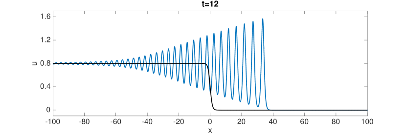
Figure 1: In black the initial data (a smooth step) and in blue KdV solution at time $t=12$ and $\epsilon=1$. One can clearly see the height of the rightmost oscillation (approximately a soliton) is about two times the height of the initial step

Using the relation $x_{+}(t)=4ct$, the limit of the elliptic solution (40) when $\beta_{2}\to\beta_{1}\to c$ gives

$$u(x,t,\epsilon)\simeq 2c\,\,{\rm sech}^{2}\left[\dfrac{x-x_{+}(t)}{\epsilon}\sqrt{c}+\dfrac{1}{2}\log\left(\dfrac{16c}{c-\beta_{2}}\right)+\dfrac{\tilde{\phi}_{0}}{\epsilon}\right],$$ (41)

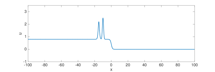
Figure 2: On top the step-like initial data and on bottom the solution at time $t=12$. One can clearly see the soliton region containing two solitons and the collision-less shock region where modulated oscillations are formed.

where the logarithmic term is due to the expansion of the complete elliptic integral $K(m)$ as in (27) and $c-\beta_{2}=O(\epsilon)$. The determination of the limiting value of the phase $\tilde{\phi}_{0}$ requires a deeper analysis [11]. The important feature of the above formula is that if the argument of the $\rm{sech}$ term is approximately zero near the point $x_{+}(t)$, then the height of the rightmost oscillation is twice the initial step $c$. This occurs for a single step initial data (see figure 1) while for step-like initial data as in figure 2 this is clearly less evident.

The Gurevich Pitaevsky problem has been studied also for perturbations of the KdV equation with forcing, dissipative or conservative non integrable terms [24],[37],[38] and applied to the evolution of solitary waves and undular bores in shallow-water flows over a gradual slope with bottom friction [25].

3.1 Long time asymptotics

The study of the long time asymptotic of the KdV solution was initiated around 1973 with the work of Gurevich and Pitaevski [31] for step-initial data and Ablowitz and Newell [1] for rapidly decreasing initial data. By that time it was clear that for rapidly decreasing initial data the solution of the KdV equation splits into a number of solitons moving to the right and a decaying radiation moving to the left. The first numerical evidence of such behaviour was found by Zabusky and Kruskal [42]. The first mathematical results were given by Ablowitz and Newell [1] and Tanaka [51] for rapidly decreasing initial data. Precise asymptotics on the radiation part were first obtained by Zakharov and Manakov, [61], Ablowitz and Segur [2] and Buslaev and Sukhanov [7], Venakides [57]. Rigorous mathematical results were also obtained by Deift and Zhou [17], inspired by earlier work by Its [36]; see also the review [14] and the book [49] for the history of the problem. In [2], [32] the region with modulated oscillations of order O(1) emerging in the long time asymptotics was called collisionless shock region. In the physics and applied mathematics literature such oscillations are also called dispersive shock waves, dissipationless shock wave or undular bore. The phase of the oscillations was obtained in [16]. Soon after the Gurevich and Pitaevski’s paper, Khruslov [40] studied the long time asymptotic of KdV via inverse scattering for step-like initial data. In more recent works, using the techniques introduced in [17], the long time asymptotic of KdV solution has been obtained for step like initial data improving some error estimates obtained earlier and with the determination of the phase $\phi_{0}$ of the oscillations [23], see also [3]. Long time asymptotic of KdV with different boundary conditions at infinity has been considered in [5]. The long time asymptotic of the expansive step has been considered in [46].

Here we report from [23] about the long time asymptotics of KdV with step like initial data $f(x)$, namely initial data converging rapidly to the limits

$$\left\{\begin{array}[]{ll}f(x)\to 0&\mbox{for}\;\;x\to+\infty\\ f(x)\to c>0&\mbox{for}\;\;x\to-\infty,\end{array}\right.$$ (42)

but in the finite region of the $x$ plane any kind of regular behaviour is allowed. The initial data has to satisfy the extra technical assumption of being sufficiently smooth. Then the asymptotic behaviour of $u(x,t;\epsilon)$ for fixed $\epsilon$ and $t\to\infty$ has been obtained applying the Deift-Zhou method in [17]:

• in the region $x/t>4c+\delta$, for some $\delta>0$, the solution is asymptotically given by the sum of solitons if the initial data contains solitons otherwise the solution is approximated by zero at leading order;

• in the region $-6c+\delta_{1}<x/t<4c-\delta_{2}$, for some $\delta_{1},\delta_{2}>0$, (collision-less shock region) the solution $u(x,t;\epsilon)$ is given by the modulated travelling wave (40), or using $\vartheta$-function by (33), namely

  $$u(x,t;\epsilon)=\beta_{2}(x,t)-c+2c\dfrac{E(m)}{K(m)}+\dfrac{2k^{2}}{(2\pi)^{2}}\left(\log\vartheta\left(\dfrac{kx-\omega t+\phi_{0}}{2\pi\epsilon};\tau\right)\right)^{\prime\prime}+o(1)$$ (43)

  where

  $$k=\pi\dfrac{\sqrt{c}}{K(m)},\quad\omega=2k(c+\beta_{2}),\quad m=\dfrac{\beta_{2}(x,t)}{c}$$

  with $\beta_{2}=\beta_{2}(x,t)$ determined by (39). In the above formula the prime in the $\log\vartheta$ means derivative with respect to the argument, namely $(\log\vartheta(z_{0};\tau))^{\prime\prime}=\dfrac{d^{2}}{dz^{2}}\log\vartheta(z+z_{0};\tau))|_{z=0}$. The phase $\phi_{0}$ is

  $$\phi_{0}=\dfrac{k}{\pi}\int_{\beta_{2}}^{c}\dfrac{\log|\bar{T}(i\sqrt{z})T_{1}(i\sqrt{z})|dz}{\sqrt{z(c-z)(z-\beta_{2})}},$$ (44)

  where $T$ and $T_{1}$ are the transmission coefficients of the Schrödinger equation $\epsilon^{2}\dfrac{d^{2}}{dx^{2}}\Psi+f(x)\Psi=-\lambda\Psi$ from the right and left respectively.

  The remarkable feature of formula (43) is that the description of the collision-less shock region for step-like initial data coincides with the formula obtained by Gurevich and Pitaevsky for the single step initial data (37) up to a phase factor. Indeed the initial data is entering explicitly through the transmission coefficients only in the phase $\phi_{0}$ of the oscillations.

• In the region $x/t<-6t-\delta_{3}$, for some constant $\delta_{3}>0$, the solution is asymptotically close to the background $c$ up to a decaying linear oscillatory term.

We remark that the higher order correction terms of the KdV solution in the large $t$ limit can be found in [2], [7], [23], [61]. For example in the region $x<-6tc$ the solution is asymptotically close to the background $c$ up to a decaying linear oscillatory term. We also remark that the boundaries of the above three regions of the $(x,t)$ plane have escaped our analysis. In such regions the asymptotic description of the KdV solution is given by elementary functions or Painlevé trascendents see [50] or the more recent work [6].

The technique introduced by Deift-Zhou [17] to study asymptotics for integrable equations has proved to be very powerful and effective to study asymptotic behaviour of many other integrable equations like for example the semiclassical limit of the focusing nonlinear Schrödinger equation [39], the long time asymptotics of the Camassa-Holm equation [6] or the long time asymptotic of the perturbed defocusing nonlinear Schrödinger equation [18].

3.2 Small $\epsilon$ asymptotic

The idea of the formation of an oscillatory structure in the limit of small dispersion of a dispersive equation belongs to Sagdeev [48]. Gurevish and Pitaevskii in 1973 called the oscillations, arising in the small dispersion limit of KdV, dispersive shock waves in analogy with the shock waves appearing in the zero dissipation limit of the Burgers equation. A very recent experiment in a water tank has been set up where the dispersive shock waves have been reproduced [55].

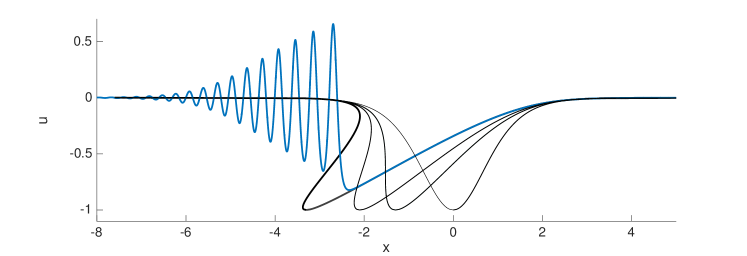
Figure 3: In blue the solution of the KdV equation for the initial data $f(x)=-{\rm sech}^{2}(x)$ at the time $t=0.55$ for $\epsilon=10^{-1}$. In black the (multivalued) solution of the Hopf equation for the same initial data and for several times: $t=0$, $t=t_{c}=0.128$, $t=0.35$ and $t=0.55$.

The main steps for the description of the dispersive shock waves are the following:

• as long as the solution of the Cauchy problem for Hopf equation $v_{t}+6vv_{x}=0$ with the initial data $v(x,0)=f(x)$ exists, then the solution of the KdV equation $u(x,t;\epsilon)=v(x,t)+O(\epsilon^{2})$. Generically the solution of the Hopf equation obtained by the method of characteristics

  $$v(x,t)=f(\zeta),\quad x=f(\zeta)t+\zeta,$$ (45)

  develops a singularity when the function $\zeta=\zeta(x,t)$ given implicitly by the map $x=f(\zeta)t+\zeta$ is not uniquely defined. This happens at the first time when $f^{\prime}(\zeta)t+1=0$ and $f^{\prime\prime}(\zeta)=0$ (see Figure 3). These two equations and (45) fix uniquely the point $(x_{c},t_{c})$ and $u_{c}=v(x_{c},t_{c})$. At this point, the gradient blow up: $v_{x}(x,t)|_{x_{c},t_{c}}\to\infty$.

• The solution of the KdV equations remains smooth for all positive times. Around the time when the solution of the Hopf equation develops its first singularity at time $t_{c}$, the KdV solution, in order to compensate the formation of the strong gradient, starts to oscillate, see Figure 3. For $t>t_{c}$ the solution of the KdV equation $u(x,t;\epsilon)$ is described as $\epsilon\to 0$ as follows:

  • there is a cusp shape region of the $(x,t)$ plane defined by $x_{-}(t)<x<x_{+}(t)$ with $x_{-}(t_{c})=x_{+}(t_{c})=x_{c}$. Strictly inside the cusp, the solution $u(x,t;\epsilon)$ has an oscillatory behaviour which is asymptotically described by the travelling wave solution (33) where the parameters $\beta_{j}=\beta_{j}(x,t)$, $j=1,2,3$, evolve according to the Whitham modulation equations.

  • Strictly outside the cusp-shape region the KdV solution is still approximated by the solution of the Hopf equation, namely $u(x,t;\epsilon)=v(x,t)+O(\epsilon^{2})$.

Later the mathematicians Lax-Levermore [44] and Venakides [58], [59] gave a rigorous mathematical derivation of the small dispersion limit of the KdV equation by solving the corresponding Cauchy problem via inverse scattering and doing the small $\epsilon$ asymptotic. Then Deift, Venakides and Zhou [15] obtained an explicit derivation of the phase $\phi_{0}$. The error term $O(\epsilon^{2})$ of the expansion outside the oscillatory zone was calculated in [12]. For analytic initial data, the small $\epsilon$ asymptotic of the solution $u(x,t;\epsilon)$ of the KdV equation is given for some times $t>t_{c}$ and within a cusp $x_{-}(t)<x<x_{+}(t)$ in the $(x,t)$ plane by the formula (33) where $\beta_{j}=\beta_{j}(x,t)$ solve the Whitham modulations equations (22). The phase $\phi_{0}$ in the argument of the theta-function will be described below. In the next section we will explain how to construct the solution of the Whitham equations.

3.2.1 Solution of the Whitham equations

The solution $\beta_{1}(x,t)>\beta_{2}(x,t)>\beta_{3}(x,t)$ of the Whitham equations can be considered as branches of a multivalued function and it is fixed by the following conditions.

• Let $(x_{c},t_{c})$ be the critical point where the solution of the Hopf equation develops its first singularity and let $u_{c}=v(x_{c},t_{c})$. Then at $t=t_{c}$

  $$\beta_{1}(x_{c},t_{c})=\beta_{2}(x_{c},t_{c})=\beta_{3}(x_{c},t_{c})=u_{c};$$

• for $t>t_{c}$ the solution of the Whitham equations is fixed by the boundary value problem ( see Fig.4)

  • when $\beta_{2}(x,t)=\beta_{3}(x,t)$, then $\beta_{1}(x,t)=v(x,t)$;

  • when $\beta_{1}(x,t)=\beta_{2}(x,t)$, then $\beta_{3}(x,t)=v(x,t)$,

  where $v(x,t)$ solve the Hopf equation.

From the integrability of the KdV equation, one has the integrability of the Whitham equations [22]. This is a non trivial fact. However we give it for granted and assume that the Whitham equations have an infinite family of commuting flows:

$$\dfrac{\partial}{\partial s}\beta_{i}+w_{i}\dfrac{\partial}{\partial x}\beta_{i}=0,\quad i=1,2,3.$$

The compatibility condition of the above flows with the Whitham equations (22), implies that $\dfrac{\partial}{\partial t}\dfrac{\partial}{\partial s}\beta_{i}=\dfrac{\partial}{\partial s}\dfrac{\partial}{\partial t}\beta_{i}$. From these compatibility conditions it follows that

$$\dfrac{1}{w_{i}-w_{j}}\dfrac{\partial}{\partial\beta_{j}}w_{i}=\dfrac{1}{\lambda_{i}-\lambda_{j}}\dfrac{\partial}{\partial\beta_{j}}\lambda_{i},\;\;i\neq j$$ (46)

where the speeds $\lambda_{i}$’s are defined in (22).

Tsarev [56] showed that if the $w_{i}=w_{i}(\beta_{1},\beta_{2},\beta_{3})$ satisfy the above linear overdetermined system, then the formula

$$x=\lambda_{i}t+w_{i},\quad i=1,2,3,$$ (47)

that is a generalisation of the method of characteristics, gives a local solution of the Whitham equations (22). Indeed by subtracting two equations in (47) with different indices we obtain

$$(\lambda_{i}-\lambda_{j})t+w_{i}-w_{j}=0,\quad\mbox{or }\quad t=-\dfrac{w_{i}-w_{j}}{\lambda_{i}-\lambda_{j}}.$$ (48)

Taking the derivative with respect to $x$ of the hodograph equation (47) gives

$$\sum_{j=1}^{3}\left(\dfrac{\partial\lambda_{i}}{\partial\beta_{j}}t+\dfrac{\partial w_{i}}{\partial\beta_{j}}\right)\dfrac{\partial\beta_{j}}{\partial x}=1.$$

Substituting in the above formula the time as in (48) and using (46), one get that only the term with $j=i$ surveys, namely

$$\left(\dfrac{\partial\lambda_{i}}{\partial\beta_{i}}t+\dfrac{\partial w_{i}}{\partial\beta_{i}}\right)\dfrac{\partial\beta_{i}}{\partial x}=1.$$

In the same way, making the derivative with respect to time of (47) one obtains

$$\left(\dfrac{\partial\lambda_{i}}{\partial\beta_{i}}t+\dfrac{\partial w_{i}}{\partial\beta_{i}}\right)\dfrac{\partial\beta_{i}}{\partial t}+\lambda_{i}=0.$$

The above two equations are equivalent to the Whitham system (22). The transformation (47) is called also hodograph transform. To complete the integration one needs to specify the quantities $w_{i}$ that satisfy the linear overdetermined system (46). As a formal ansatz we look for a conservation law of the form

$$\partial_{s}k+\partial_{x}(kq)=0,$$

with $k$ the wave number and the function $q=q(\beta_{1},\beta_{2},\beta_{3})$ to be determined (recall that $q=2(\beta_{1}+\beta_{2}+\beta_{3})$ for the Whitham equations (22)). Assuming that the $\beta_{i}$ evolves independently, such ansatz gives $w_{i}$ of the form

$$w_{i}=\frac{1}{2}\left(v_{i}-2\sum_{k=1}^{3}\beta_{k}\right)\frac{\partial q}{\partial\beta_{i}}+q,\quad i=1,2,3.$$ (49)

Plugging the expression (49) into (46), one obtains equations for the function $q=q(\beta_{1},\beta_{2},\beta_{3})$

$$\dfrac{\partial q}{\partial\beta_{i}}-\dfrac{\partial q}{\partial\beta_{j}}=2(\beta_{i}-\beta_{j})\dfrac{\partial^{2}q}{\partial\beta_{i}\partial\beta_{j}},i\neq j,\;i,j=1,2,3.$$ (50)

Such system of equations is a linear over-determined system of Euler-Poisson Darboux type and it was obtained in [33] and [53]. The boundary conditions on the $\beta_{i}$ specified at the beginning of the section fix uniquely the solution. The integration of (50) was performed for particular initial data in several different works (see e.g. [37], or [47], [33]) and for general smooth initial data in [53],[54]. The boundary conditions require that when $\beta_{1}=\beta_{2}=\beta_{3}=\beta$, then $q(\beta,\beta,\beta)=h_{L}(\beta)$ where $h_{L}$ is the inverse of the decreasing part of the initial data $f(x)$. The resulting function $q(\beta_{1},\beta_{2},\beta_{3})$ is [53]

$$q(\beta_{1},\beta_{2},\beta_{3})=\frac{1}{2\sqrt{2}\pi}\int_{-1}^{1}\int_{-1}^{1}d\mu d\nu\frac{h_{L}(\frac{1+\mu}{2}(\frac{1+\nu}{2}\beta_{1}+\frac{1-\nu}{2}\beta_{2})+\frac{1-\mu}{2}\beta_{3})}{\sqrt{1-\mu}\sqrt{1-\nu^{2}}}.$$ (51)

For initial data with a single negative hump, such formula is valid as long as $\beta_{3}>f_{min}$ which is the minimum value of the initial data. When $\beta_{3}$ goes beyond the hump one needs to take into account also the increasing part $h_{R}$ of the inverse the initial data $f$, namely [54]

$$q(\beta_{1},\beta_{2},\beta_{3})=\frac{1}{2\pi}\int_{\beta_{2}}^{\beta_{1}}\dfrac{d\lambda\left(\displaystyle\int_{\beta_{3}}^{-1}\frac{d\xi h_{R}(\xi)}{\sqrt{\lambda-\xi}}+\displaystyle\int_{-1}^{\lambda}\frac{d\xi h_{L}(\xi)}{\sqrt{\lambda-\xi}}\right)}{\sqrt{(\beta_{1}-\lambda)(\lambda-\beta_{2})(\lambda-\beta_{3})}}.$$ (52)

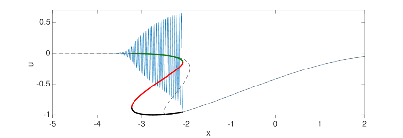
Figure 4: The thick line (green, red and black) shows the solution of the Whitham equations $\beta_{1}(x,t)\geq\beta_{2}(x,t)\geq\beta_{3}(x,t)$ at $t=0.4$ as branches of a multivalued function for the initial data $f(x)=-{\rm sech}^{2}(x)$. At this time, $\beta_{3}$ goes beyond the negative hump of the initial data and formula (52) has been used. The solution of the Hopf equation including the multivalued region is plotted with a dashed grey line, while the solution of the KdV equation for $\epsilon=10^{-2}$ is plotted with a blue line. We observe that the multivalued region for the Hopf solution is sensible smaller then the region where the oscillations develops, while the Whitham zone is slightly smaller.

Equations (47) define $\beta_{j}$, $j=1,2,3$, in an implicit way as a function of $x$ and $t$. The actual solvability of (47) for $\beta_{j}=\beta_{j}(x,t)$ was obtained in a series of papers by Fei-Ran Tian [52] [54] (see Fig. 4). The Whitham equations are a systems of hyperbolic equations, and generically their solution can suffer blow up of the gradients in finite time. When this happen the small $\epsilon$ asymptotic of the solution of the KdV equation is described by higher order $\theta$-functions and the so called multi-phase Whitham equations [27]. So generically speaking the solvability of system (47) is not an obvious fact. The main results of [52],[53] concerning this issue are the following:

• if the decreasing part of the initial data, $h_{L}$ is such that $h^{\prime\prime\prime}_{L}(u_{c})<0$ (generic condition) then the solution of the Whitham equation exists for short times $t>t_{c}$.

• If furthermore, the initial data $f(x)$ is step-like and non increasing, then under some mild extra assumptions, the solution of the Whitham equations exists for short times $t>t_{c}$ and for all times $t>T$ where $T$ is a sufficiently large time.

These results show that the Gurevich Pitaevski description of the dispersive shock waves is generically valid for short times $t>t_{c}$ and, for non increasing initial data, for all times $t>T$ where $T$ is sufficiently large. At the intermediate times, the asymptotic description of the KdV solution is generically given by the modulated multiphase solution of KdV (quasi-periodic in $x$ and $t$ ) where the wave parameters evolve according to the multi-phase Whitham equations [27]. The study of these intermediate times has been considered in [30], [4],[3].

To complete the description of the dispersive shock wave we need to specify the phase of the oscillations in (54). Such phase was derived in [15] and takes the form

$$\phi_{0}=-kq,$$ (53)

where $k=\dfrac{\pi\sqrt{\beta_{1}-\beta_{3}}}{K(m)}$ is the wave number and the function $q=q(\beta_{1},\beta_{2},\beta_{3})$ has been defined in (51) or (52). The simple form (53) of the phase was obtained in [28]. Finally the solution of the KdV equation $u(x,t;\epsilon)$ as $\epsilon\to 0$ is described as follows

• in the region strictly inside the cusp $x_{-}(t)<x<x_{+}(t)$ it is given by the asymptotic formula

  $$u(x,t,\epsilon)=\beta_{1}+\beta_{2}+\beta_{3}+2\alpha+2\epsilon^{2}\frac{\partial^{2}}{\partial x^{2}}\log\vartheta\left(\dfrac{kx-\omega t-kq)}{2\pi\epsilon};\tau\right)+O(\epsilon)$$ (54)

  where $\beta_{j}=\beta_{j}(x,t)$ is the solution of the Whitham equation constructed in this section. The wave number $k$, the frequency $\omega$ and the quantities $\tau$ and $\alpha$ are defined in (31), (34) and (24) respectively and $q$ is defined in (51) and (52). When performing the $x$-derivative in (54) observe that

  $$\partial_{x}(kx-\omega t-kq)=k,$$

  because of (47) and (49).

• For $x>x_{+}(t)+\delta$ and $x<x_{-}(t)-\delta$ for some positive $\delta>0$, the KdV solution is approximated by

  $$u(x,t,\epsilon)=v(x,t)+O(\epsilon^{2})$$

  where $v(x,t)$ is the solution of the Hopf equation.

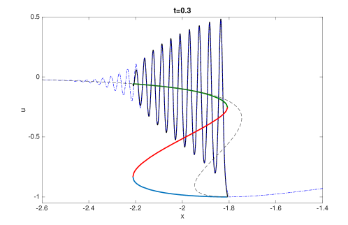
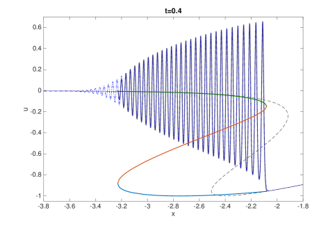
Figure 5: The solution of the KdV equation and its approximations for the initial data $f(x)=-{\rm sech}^{2}(x)$ and $\epsilon=10^{-2}$ at two different times $t=0.3$ and $t=0.4$. The blu dash-dot line is the KdV solution, the black line is the elliptic asymptotic formula (54) which is on top of the KdV solution, the black dash line is the solution of the Hopf equation while the green, red and aviation blue lines are the solution of the Whitham equations $\beta_{1}\geq\beta_{2}\geq\beta_{3}$.

Let us stress the meaning of the formula (54): such formula shows that the leading order behaviour of the KdV solution $u(x,t;\epsilon)$ in the limit $\epsilon\to 0$ and for generic initial data is given in a cusp-shape region of the $(x,t)$ plane by the periodic travelling wave of KdV. However to complete the description one still needs to solve an initial value problem, for three hyperbolic equations, namely the Whitham equations, but the gain is that these equations are independent from $\epsilon$.

A first approximation of the boundary $x_{\pm}(t)$ of the oscillatory zone for $t-t_{c}$ small, has been obtained in [28] by taking the limit of (47) when $\beta_{1}=\beta_{2}$ and $\beta_{2}=\beta_{3}$. This gives

$$x_{+}(t)\simeq x_{c}+6u_{c}(t-t_{c})+\dfrac{4\sqrt{10}}{3\sqrt{-h_{L}^{\prime\prime\prime}(u_{c})}}(t-t_{c})^{\frac{3}{2}},$$

$$x_{-}(t)\simeq x_{c}+6u_{c}(t-t_{c})-\dfrac{36\sqrt{2}}{\sqrt{-h_{L}^{\prime\prime\prime}(u_{c})}}(t-t_{c})^{\frac{3}{2}},$$

where $h_{L}$ is the decreasing part of the initial data. Such formulas coincide with the one obtained in [31] for cubic initial data.

We conclude pointing out that in [28] a numerical comparison of the asymptotic formula (54) with the actual KdV solution $u(x,t;\epsilon)$ has been considered for the intial data $f(x)=-\mbox{sech}^{2}x$. Such numerical comparison has shown the existence of transition zones between the oscillatory and non oscillatory regions that are described by Painlevé trascendant and elementary functions [9],[10],[11]. Looking for example to Fig. 5 it is clear that the KdV oscillatory region is slightly larger then the region described by the elliptic asymptotic (54) where the oscillations are confined to $x_{-}(t)\leq x\leq x_{+}(t)$.

Of particular interest is the solution of the KdV equation near the region where the oscillations are almost linear, namely near the point $x_{-}(t)$. It is known [52, 30] that taking the limit of the hodograph transform (47) when $\beta_{2}=\beta_{3}=\xi$ and $\beta_{1}=v$, one obtains the system of equations

$$\left\{\begin{array}[]{ll}&x_{-}(t)=6tv(t)+h_{L}(v(t)),\\ &6t+\phi(\xi(t);v(t))=0,\\ &\partial_{\xi}\phi(\xi(t);v(t))=0,\end{array}\right.$$ (58)

that determines uniquely $x_{-}(t)$ and and $v(t)>\xi(t)$. In the above equation the function

$$\phi(\xi;v)=\dfrac{1}{2\sqrt{v-\xi}}\int_{\xi}^{v}\dfrac{h^{\prime}_{L}(y)dy}{\sqrt{y-\xi}},$$ (59)

and $h_{L}$ is the decreasing part of the initial data. The behaviour of the KdV solution is described near the edge $x_{-}(t)$ by linear oscillations, where the envelope of the oscillations is given by the Hasting Mcleod solution to the Painlevé II equation:

$$q^{\prime\prime}(s)=sq+2q^{3}(s).$$ (60)

The special solution in which we are interested, is the Hastings-McLeod solution [34] which is uniquely determined by the boundary conditions

$$q(s)=\sqrt{-s/2}(1+o(1)), s\to-\infty$$ as , (61)

$$q(s)=\mbox{Ai}(s)(1+o(1)), s\to+\infty$$ as , (62)

where $\mbox{Ai}(s)$ is the Airy function. Although any Painlevé II solution has an infinite number of poles in the complex plane, the Hastings-McLeod solution $q(s)$ is smooth for all real values of $s$ [34] .

The KdV solution near $x_{-}(t)$ and in the limit $\epsilon\to 0$ in such a way that

$$\lim\limits_{\begin{subarray}{c}\epsilon\to 0\\ x\to x_{-}(t)\end{subarray}}\dfrac{x-x^{-}(t)}{\epsilon^{2/3}},$$

remains finite, is given by [10]

$$u(x,t,\epsilon)=v(t)-\dfrac{4\epsilon^{1/3}}{c^{1/3}}q\left(s(x,t,\epsilon)\right)\cos\left(\frac{\Theta(x,t)}{\epsilon}\right)+O(\epsilon^{\frac{2}{3}}).$$ (63)

where

$$\Theta(x,t)=2\sqrt{v-\xi}(x-x^{-})+2\int_{\xi}^{v}(h_{L}^{\prime}(y)+6t)\sqrt{y-\xi}dy$$

and

$$c=-\sqrt{v-\xi}\dfrac{\partial^{2}}{\partial\xi^{2}}\phi(\xi;v)>0,\qquad s(x,t,\epsilon)=-\frac{x-x_{-}(t)}{c^{1/3}\sqrt{v-\xi}\,\epsilon^{2/3}}.$$

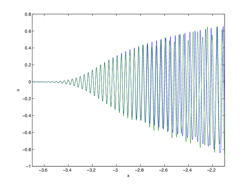
Figure 6: The solution of the KdV equation in blue and its approximation (63) in green for the initial data $f(x)=-{\rm sech}^{2}(x)$ and $\epsilon=10^{-2}$ at $t=0.4$. One can see that the green and blue lines are completely overlapped when the oscillations are small.

Note that the leading order term in the expansion (63) of $u(x,t,\epsilon)$ is given by $v(t)$ that solves the Hopf equation while the oscillatory term is of order $\epsilon^{1/3}$ with oscillations of wavelength proportional to $\epsilon$ and amplitude proportional to the Hastings-McLeod solution $q$ of the Painlevé II equation. From the practical point of view it is easier to use formula (63), then (54) since one needs to solve only an ODE (the Painlevé II equation) and three algebraic equations, namely (58). One can see from figure (6) that the asymptotic formula (63) gives a good approximation (up to an error $O(\epsilon^{\frac{2}{3}})$) of the KdV solution near the leading edge where the oscillations are linear, while inside the Whitham zone, it gives a qualitative description of the oscillations [29].

Another interesting asymptotic regime is obtained when one wants to describe the first few oscillations of the KdV solution in the small dispersion limit. In this case the so called Painlevé I2 asymptotics should be used. Furthermore we point out that it is simpler to solve one ODE, rather then the Whitham equations. For example, near the critical point $x_{c}$ and near the critical time the following asymptotic behaviour has been conjectured in [20] and proved in [9]

$$u(x,t,\epsilon)\simeq u_{c}+\left(\dfrac{2\epsilon^{2}}{\sigma^{2}}\right)^{1/7}U\left(\dfrac{x-x_{c}-6u_{c}(t-t_{c})}{(8\sigma\epsilon^{6})^{\frac{1}{7}}};\dfrac{6(t-t_{c})}{(4\sigma^{3}\epsilon^{4})^{\frac{1}{7}}}\right)+O\left(\epsilon^{4/7}\right),$$ (64)

where $\sigma=-h_{L}^{\prime\prime\prime}(u_{c})$, and $U=U(X,T)$ is the unique real smooth solution to the fourth order ODE [13]

$$X=T\,U-\left[\dfrac{U^{3}}{6}+\dfrac{1}{24}(U_{X}^{2}+2U\,U_{XX})+\frac{1}{240}U_{XXXX}\right],$$ (65)

which is the second member of the Painlevé I hierarchy (PI2 ). The relevant solution is uniquely [CL] characterized by the asymptotic behavior

$$U(X,T)=\mp(6|X|)^{1/3}\mp\frac{1}{3}6^{2/3}T|X|^{-1/3}+O(|X|^{-1}),\qquad\mbox{as $X\to\pm\infty$,}$$ (66)

for each fixed $T\in\mathbb{R}$. Such Painlevé solution matches, the elliptic solution (54) for the cubic inital data $f(x)=-x^{\frac{1}{3}}$ for large times [8]. Such solution of the PI2 has been conjectured to describe the initial time of the formation of dispersive shock waves for general Hamiltonian perturbation of hyperbolic equations [21].

We conclude by stressing that the asymptotic descriptions reviewed in this chapter for the KdV equation can be developed for other integrable equations like the nonlinear Schrödinger equation, [39] the Camass-Holm equation [6] or the modified KdV equation [41].

References

• [1] Ablowitz, M. J. and Newell, A. C. The decay of the continuous spectrum for solutions of the Korteweg-de Vries equation. J. Mathematical Phys. 14 (1973), 1277 - 1284.
• [2] Ablowitz, M. J. and Segur, H. Asymptotic solutions of the Korteweg-de Vries equation. Stud. Appl. Math. 57 (1977), 13 - 44.
• [3] Ablowitz, M.J. and Baldwin, D. E. Interactions and asymptotics of dispersive shock waves Korteweg-de Vries equation. Phys. Lett. A 377 (2013), no. 7, 555 - 559.
• [4] Ablowitz, M. J.; Baldwin, D. E.; Hoefer, M. A. Soliton generation and multiple phases in dispersive shock and rarefaction wave interaction. Phys. Rev. E (3) 80 (2009), no. 1, 016603, 5 pp.
• [5] Bikbaev, R. F. and Sharipov, R. A. The asymptotic behavior, as $t\to\infty$ of the solution of the Cauchy problem for the Korteweg de Vries equation in a class of potentials with finite-gap behavior as $\to\pm\infty$. Theoret. and Math. Phys. 78 (1989), no. 3, 244 - 252
• [6] Boutet de Monvel, A.; Its, A.; Shepelsky, D. Painlevé-type asymptotics for the Camassa-Holm equation. SIAM J. Math. Anal. 42 (2010), no. 4, 1854 - 1873.
• [7] Buslaev, V.S. and Sukhanov, V.V., Asymptotic behavior of solutions of the Korteweg de Vries equation. J. Sov. Math. 34 (1986), 1905-1920 (in English).
• [8] Claeys, T. Asymptotics for a special solution to the second member of the Painlev I hierarchy. J. Phys. A 43 (2010), no. 43, 434012, 18 pp.
• [9] Claeys, T. and Grava, T. Solitonic asymptotics for the Korteweg-de Vries equation in the small dispersion limit. SIAM J. Math. Anal. 42 (2010), no. 5, 2132 - 2154.
• [10] Claeys, T.; Grava, T. Painlevé II asymptotics near the leading edge of the oscillatory zone for the Korteweg-de Vries equation in the small-dispersion limit. Comm. Pure Appl. Math. 63, (2010), no. 2, 203 - 232.
• [11] Claeys, T. and Grava, T. Universality of the break-up profile for the KdV equation in the small dispersion limit using the Riemann-Hilbert approach. Comm. Math. Phys. 286 (2009), no. 3, 979 - 1009.
• [12] Claeys, T. and Grava, T. The KdV hierarchy: universality and a Painlevé transcendent. Int. Math. Res. Not. IMRN 22, (2012) 5063 - 5099.
• [13] Claeys, T. and Vanlessen, M. The existence of a real pole-free solution of the fourth order analogue of the Painlev I equation. Nonlinearity 20 (2007), no. 5, 1163 - 1184.
• [14] Deift, P. A.; Its, A. R.; Zhou, X. Long-time asymptotics for integrable nonlinear wave equations. Important developments in soliton theory, 181 - 204, Springer Ser. Nonlinear Dynam., Springer, Berlin, 1993.
• [15] Deift, P.; Venakides S.; Zhou, X., New result in small dispersion KdV by an extension of the steepest descent method for Riemann-Hilbert problems. IMRN 6, (1997), 285 - 299.
• [16] Deift, P.; Venakides, S.; Zhou, X. The collisionless shock region for the long-time behavior of solutions of the KdV equation. Comm. Pure Appl. Math. 47, (1994), no. 2, 199 - 206.
• [17] Deift, P.; Zhou, X. A steepest descent method for oscillatory Riemann-Hilbert problems. Asymptotics for the MKdV equation. Ann. of Math. (2) 137 (1993), no. 2, 295 - 368.
• [18] Deift, P.; Zhou, X. Perturbation theory for infinite-dimensional integrable systems on the line. A case study. Acta Math. 188 (2002), no. 2, 163 - 262.
• [19] Dobrohotov, S. Ju.; Maslov, V. P. Finite-zone almost periodic solutions in WKB-approximations. Current problems in mathematics, Vol. 15, pp. 3 94, 228, Akad. Nauk SSSR, Moscow, 1980.
• [20] B. Dubrovin, On Hamiltonian Perturbations of Hyperbolic Systems of Conservation Laws, II: Universality of
• [21] Dubrovin, B.; Grava, T.; Klein, C.; Moro, A. On critical behaviour in systems of Hamiltonian partial differential equations. J. Nonlinear Sci. 25 (2015), no. 3, 631 - 707.
• [22] Dubrovin, B.; Novikov, S. P. Hydrodynamic of weakly deformed soliton lattices. Differential geometry and Hamiltonian theory. Russian Math. Surveys 44 (1989), no. 6, 35 - 124.
• [23] Egorova, I.; Gladka, Z.; Kotlyarov, V.; Teschl, G. Long-time asymptotics for the Korteweg de Vries equation with step-like initial data. Nonlinearity 26 (2013), no. 7, 1839 - 1864.
• [24] El, G. A. Resolution of a shock in hyperbolic systems modified by weak dispersion. Chaos 15 (2005), no. 3, 037103, 21 pp.
• [25] El, G. A.; Grimshaw, R. H. J.; Kamchatnov, A. M. Analytic model for a weakly dissipative shallow-water undular bore. Chaos 15 (2005), no. 3, 037102, 13 pp.
• [26] Gardner C. S.; Green J. M; Kruskal M. D.; Miura R. M. Phys. Rev. Lett. 19 (1967), 1095.
• [27] Flaschka, H.; Forest, M.; McLaughlin, D. H., Multiphase averaging and the inverse spectral solution of the Korteweg-de Vries equations. Comm. Pure App. Math. 33 (1980), 739-784.
• [28] Grava, T. and Klein, C. Numerical solution of the small dispersion limit of Korteweg-de Vries and Whitham equations. Comm. Pure Appl. Math. 60 (2007), no. 11, 1623 - 1664.
• [29] Grava, T. and Klein, C. A numerical study of the small dispersion limit of the Korteweg-de Vries equation and asymptotic solutions. Phys. D 241 (2012), no. 23-24, 2246 2264.
• [30] Grava, T. and Tian, Fei-Ran, The generation, propagation, and extinction of multiphases in the KdV zero-dispersion limit. Comm. Pure Appl. Math. 55 (2002), no. 12, 1569 - 1639.
• [31] Gurevich A. V. and Pitaevskii L. P., Decay of initial discontinuity in the Korteweg de Vries equation. JETP Lett. 17 (1973) 193 - 195.
• [32] Gurevich A. V. and Pitaevskii L. P., Nonstationary structure of a collisionless shock wave. Sov. Phys. JETP 38 (1974) 291- 297.
• [33] Gurevich, A. V., Krylov, A. L and El, G. A. Evolution of a Riemann wave in dispersive hydrodynamics. Soviet Phys. JETP 74 (1992), no. 6, 957 - 962.
• [34] Hastings, S.P. and McLeod J.B., A boundary value problem associated with the second Painlevé transcendent and the Korteweg-de Vries equation, Arch. Rational Mech. Anal. 73 (1980), 31-51.
• [35] Its, A. R.; Matveev, V. B. Hill operators with a finite number of lacunae. Functional Anal. Appl. 9 (1975), no. 1, 65 - 66.
• [36] Its, A.R. Asymptotics of solutions of the nonlinear Schrddinger equation and isomonodromic deformations of systems of linear differential. Sov. Math. Dokl. 24 (1981), 452 - 456.
• [37] Kamchatnov, A. M. Nonlinear periodic waves and their modulations. An introductory course. World Scientific Publishing Co., Inc., River Edge, NJ, 2000. xiv+383 pp. ISBN: 981-02-4407-X
• [38] Kamchatnov, A. M. On Whitham theory for perturbed integrable equations. Physica D 188, (2004) 247- 261.
• [39] Kamvissis, S.; McLaughlin, K.D. T.-R.; Miller, P. D. Semiclassical soliton ensembles for the focusing nonlinear Schr dinger equation. Annals of Mathematics Studies, 154. Princeton University Press, Princeton, NJ, 2003. xii+265 pp. ISBN: 0-691-11483-8; 0-691-11482-X
• [40] Khruslov E. Y., Decay of initial step-like perturbation of the KdV equation. JETP Lett. 21 (1975), 217 - 218.
• [41] Kotlyarov, V. and Minakov, A. Modulated elliptic wave and asymptotic solitons in a shock problem to the modified Kortweg de Vries equation. J. Phys. A 48 (2015), no. 30, 305201, 35 pp.
• [42] Kruskal, M.D.; Zabusky, N. J. Interaction of solitons in a collisionless plasma and the recurrence of initial states. Phys Rev. Lett. 15 (1965), 240 - 243.
• [43] Lawden, D. F., Elliptic functions and applications. Applied Mathematical Sciences, vol. 80, Springer-Verlag, New York, 1989.
• [44] Lax P. D. and Levermore, C. D., The small dispersion limit of the Korteweg de Vries equation, I,II,III. Comm. Pure Appl. Math. 36 (1983), 253 - 290, 571 - 593, 809 - 830.
• [45] Levermore, C.D., The hyperbolic nature of the zero dispersion KdV limit. Comm. Partial Differential Equations 13 (1988), no. 4, 495 - 514.
• [46] Leach, J. A.; and Needham, D. J. The large-time development of the solution to an initial-value problem for the Korteweg de Vries equation: I. Initial data has a discontinuous expansive step. Nonlinearity 21 (2008), 2391 - 2408.
• [47] Novikov, S.; Manakov, S. V.; Pitaevski, L. P.; Zakharov, V. E. Theory of solitons. The inverse scattering method. Translated from the Russian. Contemporary Soviet Mathematics. Consultants Bureau [Plenum], New York, 1984. xi+276 pp. ISBN: 0-306-10977-8
• [48] Sagdeev, R.Z. Collective processes and shock waves in rarefied plasma. Problems in plasma theory, M.A. Leontovich, ed., Vol 5 Atomizdat, (1964), Moscow (in Russian).
• [49] Schuur, P.C. Asymptotic analysis of soliton problems. An inverse scattering approach. Lecture Notes in Mathematics, 1232. Springer-Verlag, Berlin, 1986. viii+180 pp. ISBN: 3-540-17203-3
• [50] Segur, H.; Ablowitz, M.J. Asymptotic solutions of nonlinear evolutions equations and Painlevé transcendents. Physica D 3, 1, (1981), 165 - 184.
• [51] Tanaka, S.: Korteweg de Vries equation; asymptotic behavior of solutions. Publ. Res. Inst. Math. Sci. 10 (1975), 367 - 379.
• [52] Tian, Fei-Ran, Oscillations of the zero dispersion limit of the Korteweg de Vries equations. Comm. Pure App. Math. 46 (1993) 1093 - 1129.
• [53] Tian, Fei-Ran The Whitham-type equations and linear overdetermined systems of Euler-Poisson-Darboux type. Duke Math. J. 74 (1994), no. 1, 203 - 221.
• [54] Tian, Fei-Ran , The initial value problem for the Whitham averaged system. Comm. Math. Phys. 166 (1994), no. 1, 79 - 115.
• [55] Trillo S.; Klein M.; Clauss G.; Onorato M., Observation of dispersive shock waves developing from initial depressions in shallow water, to appear in Physica D, http://dx.doi.org/10.1016/j.physd.2016.01.007
• [56] Tsarev, S. P., Poisson brackets and one-dimensional Hamiltonian systems of hydrodynamic type. Soviet Math. Dokl. 31 (1985), 488 - 491.
• [57] Venakides S. Long time asymptotics of the Korteweg de Vries equation Trans. Am. Math. Soc. 293 (1986), 411 - 419.
• [58] Venakides, V., The zero dispersion limit of the Korteweg de Vries equation for initial potential with nontrivial reflection coefficient. Comm. Pure Appl. Math. 38 (1985), 125 - 155.
• [59] Venakides, S., The Korteweg de Vries equations with small dispersion: higher order Lax-Levermore theory. Comm. Pure Appl. Math. 43 (1990), 335 - 361.
• [60] Whitham, G. B., Linear and nonlinear waves, J.Wiley, New York, 1974.
• [61] Zakharov, V. E.; Manakov, S. V. Asymptotic behavior of non-linear wave systems integrated by the inverse scattering method. Soviet Physics JETP 44 (1976), no. 1, 106 - 112.