Optimal selection of the $k$-th best candidate

Abstract

In the subject of optimal stopping, the classical secretary problem is concerned with optimally selecting the best of $n$ candidates when their relative ranks are observed sequentially. This problem has been extended to optimally selecting the $k$-th best candidate for $k\geq 2$. While the optimal stopping rule for $k=1,2$ (and all $n\geq 2$) is known to be of threshold type (involving one threshold), we solve the case $k=3$ (and all $n\geq 3$) by deriving an explicit optimal stopping rule that involves two thresholds. We also prove several inequalities for $p(k,n)$, the maximum probability of selecting the $k$-th best of $n$ candidates. It is shown that (i) $p(1,n)=p(n,n)>p(k,n)$ for $1<k<n$, (ii) $p(k,n)\geq p(k,n+1)$, (iii) $p(k,n)\geq p(k+1,n+1)$, and (iv) $p(k,\infty):=\lim_{n\to\infty}p(k,n)$ is decreasing in $k$.

December 4, 2017

Keywords: secretary problem; best choice; backward induction; optimal stopping.

2010 Mathematics Subject Classification:	Primary 60G40
	Secondary 62L15

1 Introduction

The classical secretary problem (also known as the best choice problem) has been extensively studied in the literature on optimal stopping, which is usually described as follows. There are $n$ (fixed) candidates to be interviewed sequentially in random order for one secretarial position. It is assumed that these candidates can be ranked linearly without ties by a manager (rank 1 being the best). Upon interviewing a candidate, the manager is only able to observe the candidate’s (relative) rank among those that have been interviewed so far. The manager then must decide whether to accept the present candidate (and stop interviewing) or to reject the candidate (and continue interviewing). No recall is allowed. The object is to maximize the probability of selecting the best candidate. More precisely, let $R_{j}$, $j=1,2,\ldots,n$, be the absolute rank of the $j$-th candidate such that $(R_{1},\dots,R_{n})=\sigma_{n}$ with probability $1/n!$ for every permutation $\sigma_{n}$ of $(1,2,\dots,n)$. Define $X_{j}=|\{1\leq i\leq j:R_{i}\leq R_{j}\}|$, the relative rank of the $j$-th candidate among the first $j$ candidates. It is desired to find a stopping rule $\tau_{1,n}\in\mathcal{M}_{n}$ such that $P(R_{\tau_{1,n}}=1)=\sup_{\tau\in\mathcal{M}_{n}}P(R_{\tau}=1)$ where $\mathcal{M}_{n}$ denotes the set of all stopping rules adapted to the filtration $\{\mathcal{F}_{j}\}$, $\mathcal{F}_{j}$ being the $\sigma$-algebra generated by $X_{1},X_{2},\dots,X_{j}$. It is well known (cf. Lindley [6]) that the optimal stopping rule $\tau_{1,n}$ is of threshold type given by $\tau_{1,n}=\min\{r_{n}\leq j\leq n:X_{j}=1\}$ where $\min\emptyset:=n$ and the threshold $r_{n}:=\min\{j\geq 1:\;\sum_{i=j+1}^{n}\frac{1}{i-1}\leq 1\}$. Moreover, the maximum probability of selecting the best candidate (under $\tau_{1,n}$) is $p(1,n):=\frac{r_{n}-1}{n}\sum_{i=r_{n}}^{n}\frac{1}{i-1}$, which converges as $n\to\infty$ to $p(1,\infty):=1/e=\lim_{n\to\infty}r_{n}/n$.

A great many interesting variants of the secretary problem have been formulated and solved in the literature (cf. the review papers by Ferguson [2] and Freeman [4] and Samuels [9]), most of which are concerned with optimally selecting the best candidate or one of the $k$ best candidates. In contrast, only a few papers (cf. Rose [7], Szajowski [11] and Vanderbei [12]) considered and solved the problem of optimally selecting the second best candidate. (According to Vanderbei [12], in 1980, E.B. Dynkin proposed this problem to him with the motivating story that “We are trying to hire a postdoc and we are confident that the best candidate will receive and accept an offer from Harvard.” Thus Vanderbei [12] refers to the problem as the postdoc variant of the secretary problem.) These authors showed that the optimal stopping rule $\tau_{2,n}$ is also of threshold type given by $\tau_{2,n}=\min\{r_{n}^{\prime}\leq j\leq n:X_{j}=2\}$ with $r_{n}^{\prime}=\lceil\frac{n+1}{2}\rceil$ (the smallest integer not less than $\frac{n+1}{2}$), which attains the maximum probability of selecting the second best candidate

$$p(2,n):=P(R_{\tau_{2,n}}=2)=\sup_{\tau\in\mathcal{M}_{n}}P(R_{\tau}=2)=\frac{(r_{n}^{\prime}-1)(n-r_{n}^{\prime}+1)}{n(n-1)}.$$

Note that $p(2,\infty)=\lim_{n\to\infty}p(2,n)=1/4<1/e=p(1,\infty)$.

In this paper, we consider the problem of optimally selecting the $k$-th best candidate for general $k$. Let $p(k,n):=\sup_{\tau\in\mathcal{M}_{n}}P(R_{\tau}=k)$, the maximum probability of selecting the $k$-th best of $n$ candidates. Szajowski [11] derived the asymptotic solutions as $n\to\infty$ for $k=3,4,5$. Rose [8] dealt with the case $k=(n+1)/2$ for odd $n$, which was called the median problem and suggested by M. DeGroot with the motivation of selecting a candidate representative of the entire sequence. (The candidate of rank $k=(n+1)/2$ is, in some sense, representative of all candidates.) In the next section, we solve the case $k=3$ for all finite $n\geq 3$ by showing (cf. Theorem 2.1) that the stopping rule $\tau_{3,n}=\min\{a_{n}\leq j\leq n:X_{j}=2\}\wedge\min\{b_{n}\leq j\leq n:X_{j}=3\}$ attains the maximum probability $P(R_{\tau_{3,n}}=3)=p(3,n)$ for $n\geq 3$, where $x\wedge y:=\min\{x,y\}$ and the two thresholds $a_{n}<b_{n}$ are given in (2.8) and (2.5), respectively. In Section 3, we prove (cf. Theorems 3.1 and 3.2) that (i) $p(1,n)=p(n,n)>p(k,n)$ for $1<k<n$, (ii) $p(k,n)\geq p(k,n+1)$, (iii) $p(k,n)\geq p(k+1,n+1)$, and (iv) $p(k,\infty):=\lim_{n\to\infty}p(k,n)$ is decreasing in $k$. It is also noted (cf. Remark 3.1) that the inequality $p(k,n)\geq p(k+1,n)$ occasionally fails to hold for $k$ close to (but less than) $\lceil\frac{n}{2}\rceil$. Furthermore, we extend the result $p(1,n)=p(n,n)>p(k,n)$ for $1<k<n$ to the setting where the goal is to select a candidate whose absolute rank belongs to a prescribed subset $\Gamma$ of $\{1,\dots,n\}$ with $|\Gamma|=c\;(1\leq c<n)$ (cf. Suchwalko and Szajowski [10]). It is shown (cf. Theorem 3.3) that the probability of optimally selecting a candidate whose absolute rank belongs to $\Gamma$ is maximized when $\Gamma=\{1,\dots,c\}$ or $\Gamma=\{n-c+1,\dots,n\}$. The proofs of several technical lemmas are relegated to Section 4. Section 5 contains a computer program in Mathematica for verification of Theorem 2.1 for $3\leq n\leq 31$. It should be remarked that the optimal stopping rule is not necessarily unique. For example, a slight modification $\tau_{2,n}^{\prime}$ of the optimal stopping rule $\tau_{2,n}$ also attains the maximum probability $p(2,n)$ where $\tau_{2,n}^{\prime}\geq r_{n}^{\prime}-1$ is given by $\tau_{2,n}^{\prime}=r_{n}^{\prime}-1$ if $X_{r_{n}^{\prime}-1}=1$ and $\tau_{2,n}^{\prime}=\tau_{2,n}$ otherwise. The uniqueness issue of the optimal stopping rule is not addressed in this paper.

2 Maximizing the probability of selecting the $k$-th best candidate with $k=3$

We adopt the setup and notations in Ferguson [3, Chapter 2]. As defined in Section 1, $X_{j}$ is the relative rank of the $j$-th candidate among the first $j$ candidates and $R_{j}$ is the absolute rank. Given $X_{1}=x_{1},X_{2}=x_{2},\dots,X_{j}=x_{j}$, $1\leq j\leq n$, let $y_{j}(x_{1},x_{2},\dots,x_{j})$ be the return for stopping at stage $j$ (i.e. accepting the $j$-th candidate) and $V_{j}(x_{1},x_{2},\dots,x_{j})$ the maximum return by optimally stopping from stage $j$ onwards. In other words, $y_{j}(x_{1},x_{2},\dots,x_{j})$ is the conditional probability of $R_{j}=k$ (given $X_{i}=x_{i}$, $1\leq i\leq j$), which defines the reward function for the stopping problem of optimally selecting the $k$-th best candidate. Given $X_{i}=x_{i}$, $1\leq i\leq j$, $V_{j}(x_{1},x_{2},\dots,x_{j})$ is the (maximum) expected reward by optimally stopping from stage $j$ onwards. Then $V_{n}(x_{1},x_{2},\dots,x_{n})=y_{n}(x_{1},x_{2},\dots,x_{n})$, and

$$V_{j}\left(x_{1},\dots,x_{j}\right)=\max\left\{y_{j}(x_{1},\dots,x_{j}),E\left(V_{j+1}\left(x_{1},\dots,x_{j},X_{j+1}\right)\Big{|}X_{1}=x_{1},\dots,X_{j}=x_{j}\right)\right\},$$ (2.1)

for $j=n-1,n-2,\dots,1$. Given $X_{i}=x_{i},i=1,\dots,j$, it is optimal to stop at stage $j$ if $V_{j}\left(x_{1},x_{2},\dots,x_{j}\right)=y_{j}(x_{1},x_{2},\dots,x_{j})$ and to continue otherwise. The (optimal) value of the stopping problem is $V_{1}(1)$, i.e. $V_{1}(1)=\sup_{\tau\in\mathcal{M}_{n}}P(R_{\tau}=k)$. This formalizes the method of backward induction. See also Chow, Robbins and Siegmund [1].

It is well known that $X_{1},X_{2},\dots,X_{n}$ are independent and $X_{j}$ has a uniform distribution over $\{1,2,\dots,j\}$. Given $X_{i}=x_{i},i=1,\dots,j$, the conditional probability of $R_{j}=k$ is the same as the probability that a random sample of size $j$ contains the $k$-th best candidate whose (relative) rank in the sample is $x_{j}$; thus

$$P(R_{j}=k|X_{1}=x_{1},X_{2}=x_{2},\dots,X_{j}=x_{j})=\frac{{k-1\choose x_{j}-1}{n-k\choose j-x_{j}}}{{n\choose j}},$$ (2.2)

where we adopt the usual convention that ${m\choose\ell}=0$ for $m<\ell$.

From the independence of $X_{1},X_{2},\dots,X_{n}$, the conditional expectation on the right hand side of (2.1) reduces to $E(V_{j+1}(x_{1},x_{2},\dots,x_{j},X_{j+1}))$. Note also that $y_{j}(x_{1},\dots,x_{j})$ depends only on $x_{j}$ (cf. (2.2)), and so does $V_{j}(x_{1},\dots,x_{j})$. Hence, we have

$$V_{n}(x_{n})=y_{n}(x_{n})$$

and $$V_{j}(x_{j})=\max\left\{y_{j}(x_{j}),\frac{1}{j+1}\sum_{i=1}^{j+1}V_{j+1}(i)\right\}\;\;\mbox{for}\;\;j=n-1,n-2,\dots,1.$$ (2.3)

Thus, it is optimal to stop at the first $j$ with

$$y_{j}(x_{j})\geq\frac{1}{j+1}\sum_{i=1}^{j+1}V_{j+1}(i).$$

For the problem of optimally selecting the $k$-th best candidate with $k=3$, we have $y_{j}(x_{j})=P(R_{j}=3|X_{1}=x_{1},\dots,X_{j}=x_{j})$, which equals (cf. (2.2))

$$y_{j}(x_{j})=\begin{cases}\displaystyle\frac{j(n-j-1)(n-j)}{n(n-1)(n-2)},&\mbox{if}\;\;x_{j}=1;\\[11.38109pt] \displaystyle\frac{2j(j-1)(n-j)}{n(n-1)(n-2)},&\mbox{if}\;\;x_{j}=2;\\[11.38109pt] \displaystyle\frac{j(j-1)(j-2)}{n(n-1)(n-2)},&\mbox{if}\;\;x_{j}=3;\\[11.38109pt] 0,&\mbox{otherwise}.\end{cases}$$ (2.4)

Setting $\sum_{i=\ell}^{m}c_{i}:=0$ whenever $\ell>m$, define for $n\geq 3$,

$$b_{n} =\min\left\{j=2,3,\dots,n:\;\sum_{i=j+1}^{n}\frac{1}{i-2}\leq\frac{1}{2}\right\},$$ (2.5)

$$u_{n} =(b_{n}-2)(2n-4)\sum_{i=b_{n}}^{n}\frac{1}{i-2},$$ (2.6)

$$f_{n}(x) =3x^{2}-(1+4n)x+(n-2)b_{n}+2(n+1)+u_{n},$$ (2.7)

$$a_{n} =\min\left\{j=2,3,\dots,n:\;f_{n}(j)\leq 0\right\}.$$ (2.8)

Remark 2.1.

Note that $3\leq b_{n}\leq b_{n+1}\leq b_{n}+1$ for $n\geq 3$, implying that $f_{n}(1)>0$ for all $n\geq 3$. In order for $a_{n}$ in $(\ref{v4e4})$ to be well defined, we need to show that the second-order polynomial equation $f_{n}(x)=0$ has two real roots $x_{0}<y_{0}$ with $\lceil x_{0}\rceil\leq y_{0}$ $(\mbox{so that}\;a_{n}=\lceil x_{0}\rceil)$. For $3\leq n\leq 31$, this can be verified by numerical computations. For $n\geq 32$, we have $b_{n}<\frac{2n-1}{3}$ and $u_{n}\leq(n-2)b_{n}$ $({\it cf.}\;(\ref{ae8})\;\mbox{and}\;(\ref{ae6}))$, implying that $f_{n}(\frac{2n-1}{3})<0$ and $f_{n}(\frac{2n+2}{3})<0$. So, $x_{0}<\frac{2n-1}{3}$, implying that $\lceil x_{0}\rceil<\frac{2n+2}{3}<y_{0}$. With a little effort, it can be shown that $2\leq a_{n}\leq a_{n+1}\leq a_{n}+1$ for $n\geq 3$.

The next theorem is our main result.

Theorem 2.1.

For $n\geq 3$, we have $a_{n}<b_{n}$. Furthermore, the stopping rule

$$\tau_{3,n}=\min\{a_{n}\leq j\leq n:X_{j}=2\}\wedge\min\{b_{n}\leq j\leq n:X_{j}=3\}$$

maximizes the probability of selecting the 3rd best candidate.

Figure 1 illustrates the optimality of $\tau_{3,n}$ for the case $n=13$ with $a_{13}=7$ and $b_{13}=9$. With the help of a computer program in Mathematica, we have verified Theorem 2.1 for $3\leq n\leq 31$ by numerically evaluating $V_{j}(x_{j})$, $j=n,n-1,\dots,1$. (For completeness, the computer program is provided in Section 5.) While it seems intuitively reasonable for the optimal stopping rule $\tau_{3,n}$ to involve two thresholds for general $n$, the exact expressions for the thresholds $a_{n}$ and $b_{n}$ in (2.8) and (2.5) were found by some guesswork and tedious analysis. To prove Theorem 2.1 for $n\geq 32$, we need the following lemmas whose proofs are relegated to Section 4.

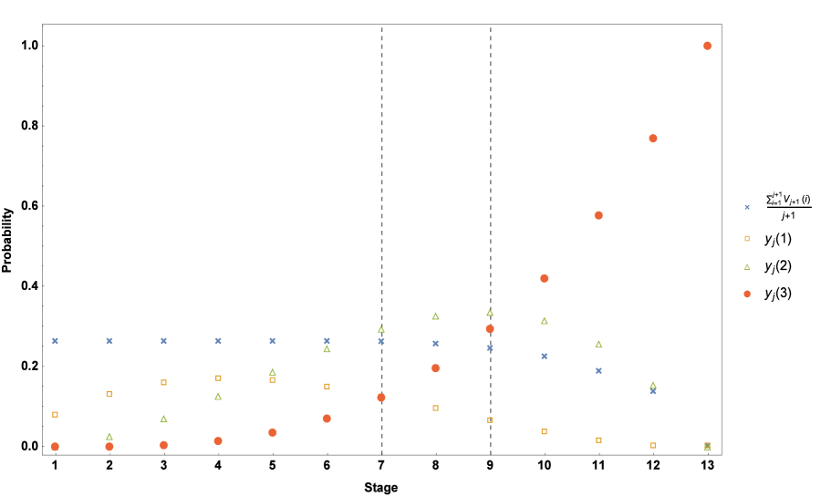
Figure 1: The optimality of $\tau_{3,13}$.

Lemma 2.1.

Let $y_{0}$ be the larger root of the second-order polynomial equation $f_{n}(x)=0$. Then for $n\geq 32$, we have (i) $a_{n}<b_{n}$; (ii) $b_{n}<y_{0}$; (iii) $a_{n}>(n+4)/3$.

Lemma 2.2.

Given $X_{1}=x_{1},X_{2}=x_{2},\dots,X_{j}=x_{j}$, let $h_{j}(x_{j})=h_{j}(x_{1},x_{2},\dots,x_{j})$ be the conditional probability of selecting the 3rd best candidate when $\tau_{3,n}$ is used for stages $j,j+1,\dots,n$. Then for $n\geq 32$,

• $$h_{j}(x_{j})=\begin{cases}\displaystyle\frac{(a_{n}-1)\left[a_{n}^{2}-(1+2n)a_{n}+(n-2)b_{n}+2(n+1)+u_{n}\right]}{n(n-1)(n-2)},&\mathrm{if}\;\;j<a_{n};\\ y_{j}(2),&\mathrm{if}\;\;j\geq a_{n}\;\mathrm{and}\;x_{j}=2;\\[2.84526pt] \displaystyle\frac{j\left[j^{2}+(1-2n)j+(n-2)b_{n}+2+u_{n}\right]}{n(n-1)(n-2)},&\mathrm{if}\;\;a_{n}\leq j\leq b_{n}-1\;\mathrm{and}\;x_{j}\neq 2;\\ y_{j}(3),&\mathrm{if}\;\;j\geq b_{n}\;\mathrm{and}\;x_{j}=3;\\[2.84526pt] \displaystyle\frac{j(j-1)}{n(n-1)(n-2)}\left[(2n-4)\sum_{i=j+1}^{n}\frac{1}{i-2}-(n-j)\right],&\mathrm{if}\;\;j\geq b_{n}\;\mathrm{and}\;x_{j}\neq 2,3.\end{cases}$$

• $$\frac{1}{j+1}\sum_{i=1}^{j+1}h_{j+1}(i)=\begin{cases}\displaystyle\frac{(a_{n}-1)\left[a_{n}^{2}-(1+2n)a_{n}+(n-2)b_{n}+2(n+1)+u_{n}\right]}{n(n-1)(n-2)},&\mathrm{if}\;\;j<a_{n};\\[11.38109pt] \displaystyle\frac{j\left[j^{2}+(1-2n)j+(n-2)b_{n}+2+u_{n}\right]}{n(n-1)(n-2)},&\mathrm{if}\;\;a_{n}\leq j\leq b_{n}-1;\\[11.38109pt] \displaystyle\frac{j(j-1)}{n(n-1)(n-2)}\left[(2n-4)\sum_{i=j+1}^{n}\frac{1}{i-2}-(n-j)\right],&\mathrm{if}\;\;b_{n}\leq j\leq n-1.\end{cases}$$

Lemma 2.3.

For $n\geq 32$, $1\leq j<a_{n}$ and $1\leq x_{j}\leq j$, we have

$$y_{j}(x_{j})<\frac{1}{j+1}\sum_{i=1}^{j+1}h_{j+1}(i).$$

Lemma 2.4.

For $n\geq 32$ and $a_{n}\leq j<b_{n}$, we have (i) $y_{j}(2)\geq\frac{1}{j+1}\sum_{i=1}^{j+1}h_{j+1}(i)$; (ii) $y_{j}(1)<\frac{1}{j+1}\sum_{i=1}^{j+1}h_{j+1}(i)$; (iii) $y_{j}(3)<\frac{1}{j+1}\sum_{i=1}^{j+1}h_{j+1}(i)$.

Lemma 2.5.

For $n\geq 32$ and $b_{n}\leq j\leq n-1$, we have (i) $y_{j}(1)<\frac{1}{j+1}\sum_{i=1}^{j+1}h_{j+1}(i)$; (ii) $y_{j}(2)\geq\frac{1}{j+1}\sum_{i=1}^{j+1}h_{j+1}(i)$; (iii) $y_{j}(3)\geq\frac{1}{j+1}\sum_{i=1}^{j+1}h_{j+1}(i)$.

Proof of Theorem 2.1.

As remarked before, the theorem has been verified for $3\leq n\leq 31$ by numerical computations. For $n\geq 32$, we need to show that $h_{j}$ satisfies

$$h_{j}(x_{j})=\max\left\{y_{j}(x_{j}),\frac{1}{j+1}\sum_{i=1}^{j+1}h_{j+1}(i)\right\}\;\mbox{for}\;\;1\leq j<n.$$ (2.9)

Since $h_{j}(x_{j})$ is the conditional probability of selecting the 3rd best candidate when $\tau_{3,n}$ is used for stages $j,\dots,n$, we have $h_{j}(x_{j})=\frac{1}{j+1}\sum_{i=1}^{j+1}h_{j+1}(i)$ if either ($j<a_{n}$) or ($a_{n}\leq j<b_{n}$ and $x_{j}\neq 2$) or ($b_{n}\leq j<n$ and $x_{j}\neq 2,3$), which together with Lemmas 2.3 – 2.5 establishes (2.9). ∎

Remark 2.2.

Let $d_{1}=\lim_{n\to\infty}a_{n}/n$ and $d_{2}=\lim_{n\to\infty}b_{n}/n$. It is shown in Section 4 that

$$d_{1}=\frac{2}{2\sqrt{e}+\sqrt{4e-6\sqrt{e}}}\approx 0.466\;\;\mbox{and}\;\;d_{2}=\frac{1}{\sqrt{e}}\approx 0.606.$$ (2.10)

It is also shown in Section 4 that as $n\to\infty$, $h_{1}(1)=p(3,n)$, the maximum probability of selecting the 3rd best candidate, tends to

$$p(3,\infty)=2d_{1}^{2}(1-d_{1})=\frac{8\left(2\sqrt{e}-2+\sqrt{4e-6\sqrt{e}}\right)}{\left(2\sqrt{e}+\sqrt{4e-6\sqrt{e}}\right)^{3}}.$$ (2.11)

Note that $p(3,\infty)\approx 0.232<0.25=p(2,\infty)$. These limiting results agree with the asymptotic solution for $k=3$ in Szajowski [11].

3 Some results on $p(k,n)$ and $p(k,\infty)$

In this section, we present several inequalities for $p(k,n)$ and $p(k,\infty):=\lim_{n\to\infty}p(k,n)$.

Theorem 3.1.

For $n\geq 3$ and $1<k<n$, we have $p(1,n)=p(n,n)>p(k,n)$.

Proof.

By symmetry, $p(1,n)=p(n,n)$. (More generally, $p(k,n)=p(n-k+1,n)$.) For the problem of selecting the $k$-th best candidate ($1<k<n$), a (non-randomized) optimal stopping rule $\tau$ is determined by a sequence of subsets $\{S_{j}\}$ such that $S_{j}\subset\{1,2,\dots,j\}\;(j=1,\dots,n)$ and $\tau=\min\{j:X_{j}\in S_{j}\}$. Since stopping at $n$ is enforced (if $\tau>n-1$), we may assume that $S_{n}=\{1,2,\dots,n\}$. Thus,

$$P(R_{\tau}=k)=p(k,n).$$ (3.1)

Define, for $j=1,\dots,n-1$,

$$S_{j}^{\prime}=\begin{cases}\emptyset,&\;\;\mbox{if}\;S_{j}=\emptyset;\\ \{1\},&\;\;\mbox{if}\;S_{j}\neq\emptyset;\end{cases}$$

and $S_{n}^{\prime}=\{1,2,\dots,n\}$. Let $\tau^{\prime}=\min\{j:X_{j}\in S_{j}^{\prime}\}$, which, as a stopping rule, may be applied to selecting the best candidate. Thus

$$P(R_{\tau^{\prime}}=1)\leq\sup_{\nu\in\mathcal{M}_{n}}P(R_{\nu}=1)=p(1,n).$$ (3.2)

Note that for $j=1,\dots,n$,

$$P(R_{j}=1,X_{j}=1)=\frac{1}{n} =P(R_{j}=k)$$

$$\geq P(R_{j}=k,X_{j}\in S_{j}).$$ (3.3)

By (2.2), given $X_{1}=x_{1},\dots,X_{j}=x_{j}$, the conditional distribution of $R_{j}$ depends only on $x_{j}$, implying that $X_{1},\dots,X_{j-1}$ and $(X_{j},R_{j})$ are independent. So if $S_{j}\neq\emptyset$,

$$P(\tau=j,R_{j}=k) =P(X_{i}\notin S_{i},\;i=1,\dots,j-1,\;X_{j}\in S_{j},R_{j}=k)$$

$$=\left[\prod_{i=1}^{j-1}P(X_{i}\notin S_{i})\right]P(X_{j}\in S_{j},R_{j}=k)$$

$$\leq\left[\prod_{i=1}^{j-1}P(X_{i}\notin S_{i}^{\prime})\right]P(X_{j}=1,R_{j}=1)$$ (3.4)

$$=P(\tau^{\prime}=j,R_{j}=1),$$

where the inequality follows from (3.3) and $|S_{i}^{\prime}|\leq|S_{i}|$ for all $i$. (If $S_{j}=\emptyset$, then $P(\tau=j,R_{j}=k)=P(\tau^{\prime}=j,R_{j}=1)=0$.) By (3.1), (3.2) and (3.4), we have

$$p(k,n)=P(R_{\tau}=k) =\sum_{j=1}^{n}P(\tau=j,R_{j}=k)$$

$$\leq\sum_{j=1}^{n}P(\tau^{\prime}=j,R_{j}=1)=P(R_{\tau^{\prime}}=1)\leq p(1,n).$$ (3.5)

It remains to show that (at least) one of the two inequalities in (3.5) is strict (so that $p(k,n)<p(1,n)$). If the stopping rule $\tau^{\prime}$ is not optimal for selecting the best candidate, then the second inequality in (3.5) is strict. Suppose $\tau^{\prime}$ is optimal for selecting the best candidate, which implies, in view of $n\geq 3$, that $S_{1}^{\prime}=\emptyset$ and $S_{n-1}^{\prime}=\{1\}$, which in turn implies that $|S_{n-1}|\geq 1$. If $|S_{n-1}|\geq 2$, then the inequality in (3.4) is strict for $j=n$, implying that the first inequality in (3.5) is strict. Suppose $S_{n-1}=\{\ell\}$ for some $\ell$. Then we have

$$P(R_{n-1}=k,X_{n-1}=\ell)=\begin{cases}\frac{n-k}{n(n-1)},&\;\;\mbox{if}\;k=\ell;\\ \frac{k-1}{n(n-1)},&\;\;\mbox{if}\;k=\ell+1;\\ 0,&\;\;\mbox{if}\;k-\ell\neq 0,1;\end{cases}$$

implying, in view of $1<k<n$, that the inequality in (3.3) is strict for $j=n-1$, which in turn implies that the inequality in (3.4) is strict for $j=n-1$. It follows that the first inequality in (3.5) is strict. The proof is complete. ∎

Theorem 3.2.

For $1\leq k\leq n$, we have $p(k,n)\geq p(k,n+1)\;(\mbox{i.e.}\;p(k,n)\;\mbox{is decreasing in}\;n)$ and $p(k,n)\geq p(k+1,n+1)$. Furthermore, $p(k,\infty):=\lim_{n\to\infty}p(k,n)$ is well defined, and $p(k,\infty)\geq p(k+1,\infty)$.

Proof.

(i) To show $p(k,n)\geq p(k,n+1)$, consider the case of selecting the $k$-th best of $n+1$ candidates. Let the random variable $I\in\{1,\dots,n+1\}$ be such that $R_{I}=n+1$ (i.e. the worst candidate is the $I$-th person to be interviewed). If $I$ is known to the manager (or more precisely, the manager knows the position of the worst candidate before the interview process begins), then the problem of optimally selecting the $k$-th best of the $n+1$ candidates is equivalent to that of optimally selecting the $k$-th best of the $n$ candidates (excluding the worst one). (Indeed, let $X_{i}^{\prime}=X_{i}$ for $1\leq i<I$ and $X_{i}^{\prime}=X_{i+1}$ for $I\leq i\leq n$. Given $I$, $X_{1}^{\prime},\dots,X_{n}^{\prime}$ are (conditionally) independent with each $X_{i}^{\prime}$ being uniform over $\{1,\dots,i\}$.) Thus, when $I$ is known to the manager, the maximum probability of selecting the $k$-th best candidate equals $p(k,n)$, which must be at least as large as $p(k,n+1)$, the maximum probability of selecting the $k$-th best of the $n+1$ candidates when $I$ is unavailable. This proves that $p(k,n)\geq p(k,n+1)$.

(ii) To show $p(k,n)\geq p(k+1,n+1)$, note that

$$p(k,n)=p(n-k+1,n)\geq p(n+1-k,n+1)=p(k+1,n+1),$$ (3.6)

where the two equalities follow from the symmetry property $p(k,n)=p(n-k+1,n)$ and the inequality follows from the decreasing property of $p(k,n)$ in $n$.

(iii) Since $p(k,n)$ is decreasing in $n$, $p(k,\infty):=\lim_{n\to\infty}p(k,n)$ is well defined. By (3.6), we have

$$p(k,\infty)=\lim_{n\to\infty}p(k,n)\geq\lim_{n\to\infty}p(k+1,n+1)=p(k+1,\infty).$$

The proof is complete. ∎

Remark 3.1.

We conjecture that the three inequalities in Theorem 3.2 are all strict. While $p(k,n)$ is decreasing in $n$, in view of $p(1,n)>p(k,n)$ for $1<k<n$ and $p(k,\infty)\geq p(k+1,\infty)$, it may be tempting to conjecture that $p(k,n)\geq p(k+1,n)$ for $1\leq k<\lceil\frac{n}{2}\rceil$. However, this inequality occasionally fails to hold for $k$ close to $(\mbox{but less than})$ $\lceil\frac{n}{2}\rceil$. Our numerical results show that the set $\{(k,n):1\leq k<\lceil\frac{n}{2}\rceil,n\leq 50,p(k,n)<p(k+1,n)\}$ consists of $(2,5),(2,7),(7,15),(9,19),(10,21),(12,25),(21,43),(22,47),(24,49)$ and $(24,50)$. Moreover, it can be shown that $p(2,n)>p(3,n)$ for all $n\geq 8$. Let $\rho=\liminf_{n\to\infty}K(n)/n$ where $K(n)=\max\{1\leq k\leq\lceil\frac{n}{2}\rceil:p(1,n)\geq p(2,n)\geq\cdots\geq p(k,n)\}$. While $0\leq\rho\leq 1/2$, it appears to be a challenging task to find the exact value of $\rho$. Our limited numerical results suggest that $\rho$ may be equal to $1/2$.

Remark 3.2.

It may be of interest to see how fast $p(k,\infty)$ tends to $0$ as $k$ increases. By considering some suboptimal rules, we have derived a crude lower bound $k^{\frac{-k}{k-1}}$ for $p(k,\infty)$. The details are omitted.

The next theorem extends Theorem 3.1 to the setting where the goal is to select a candidate whose rank belongs to a prescribed subset $\Gamma$ of $\{1,\dots,n\}$ (cf. Suchwalko and Szajowski [10]). Let

$$p(\Gamma,n)=\sup_{\tau\in\mathcal{M}_{n}}P(R_{\tau}\in\Gamma).$$

Theorem 3.3.

For any subset $\Gamma$ of $\{1,2,\dots,n\}$ with $|\Gamma|=c\;\;(1\leq c<n)$, we have

$$p(\Gamma,n)\leq p(\{1,2,\dots,c\},n)=p(\{n-c+1,\dots,n\},n).$$

In the proof below, it is convenient to take the convention that ${0\choose 0}:=1$ and ${n\choose k}:=0$ if $n<k$ or $n<0$ or $k<0$, so that

$${n\choose k}={n-1\choose k}+{n-1\choose k-1}\;\;\mbox{for}\;\;(k,n)\in\mathbb{Z}\times\mathbb{Z}\backslash\{(0,0)\},$$ (3.7)

and

$${n\choose k}\geq{n-1\choose k}+{n-1\choose k-1}\;\;\mbox{for}\;\;(k,n)\in\mathbb{Z}\times\mathbb{Z},$$ (3.8)

where $\mathbb{Z}$ is the set of all integers.

Proof of Theorem 3.3.

As in the proof of Theorem 3.1, let $\tau$ be a (non-randomized) optimal stopping rule determined by a sequence of subsets $\{S_{j}\}$ of $\{1,\dots,n\}$ such that $S_{j}\subset\{1,\dots,j\}$, $\tau=\min\{j:X_{j}\in S_{j}\}$ and $P(R_{\tau}\in\Gamma)=p(\Gamma,n)$. Again, as stopping at $n$ is enforced (if $\tau>n-1$), we may assume that $S_{n}=\{1,2,\dots,n\}$. Let $S_{j}^{\prime}=\{1,2,\dots,|S_{j}|\}$, so $|S_{j}^{\prime}|=|S_{j}|$ (in particular, $S_{j}^{\prime}=\emptyset$ if $S_{j}=\emptyset$). Let $\tau^{\prime}=\min\{j:X_{j}\in S_{j}^{\prime}\}$. Claim

$$P(R_{j}\in\{t_{1},t_{2},\dots,t_{c}\},X_{j}\in\{s_{1},s_{2},\dots,s_{d}\})\leq P(R_{j}\in\{1,2,\dots,c\},X_{j}\in\{1,2,\dots,d\})$$ (3.9)

for $1\leq d\leq j\leq n$, $1\leq c\leq n,1\leq t_{1}<t_{2}<\dots<t_{c}\leq n$, and $1\leq s_{1}<s_{2}<\dots<s_{d}\leq j$. If the claim (3.9) is true, then for $j=1,\dots,n$,

$$P(\tau=j,R_{j}\in\Gamma) =P(X_{i}\notin S_{i},\;i=1,\dots,j-1,\;X_{j}\in S_{j},R_{j}\in\Gamma)$$

$$=\left[\prod_{i=1}^{j-1}P(X_{i}\notin S_{i})\right]P(R_{j}\in\Gamma,X_{j}\in S_{j})$$

$$\leq\left[\prod_{i=1}^{j-1}P(X_{i}\notin S_{i}^{\prime})\right]P(R_{j}\in\{1,\dots,c\},X_{j}\in S_{j}^{\prime})\;\;(\mbox{by}\;(\ref{e6}))$$

$$=P(X_{i}\notin S_{i}^{\prime},i=1,\dots,j-1,X_{j}\in S_{j}^{\prime},R_{j}\in\{1,\dots,c\})$$

$$=P(\tau^{\prime}=j,R_{j}\in\{1,\dots,c\}),$$

implying that $p(\Gamma,n)=P(R_{\tau}\in\Gamma)\leq P(R_{\tau^{\prime}}\in\{1,\dots,c\})\leq p(\{1,\dots,c\},n)$.

It remains to establish (3.9). Note that

$$P(R_{j}\in\{t_{1},\dots,t_{c}\}, \;X_{j}\in\{s_{1},\dots,s_{d}\})$$

$$\leq P(R_{j}\in\{t_{1},\dots,t_{c}\})=\frac{c}{n}$$

$$=P(R_{j}\in\{1,\dots,c\})$$

$$=P(R_{j}\in\{1,\dots,c\},X_{j}\in\{1,\dots,d\})\;\;\mbox{(if}\;d\geq c),$$

showing that (3.9) holds for $d\geq c$. Since

$$P(R_{j}=a,X_{j}=b)=\frac{{a-1\choose b-1}{n-a\choose j-b}}{n{n-1\choose j-1}}\;\;\mbox{for all integers}\;\;a>0,b>0,$$

(3.9) is equivalent to

$$\sum_{i=1}^{d}\sum_{\ell=1}^{c}{t_{\ell}-1\choose s_{i}-1}{n-t_{\ell}\choose j-s_{i}}\leq\sum_{i=1}^{d}\sum_{\ell=1}^{c}{\ell-1\choose i-1}{n-\ell\choose j-i},$$ (3.10)

for $1\leq d\leq j\leq n,1\leq c\leq n,1\leq t_{1}<\cdots<t_{c}\leq n$ and $1\leq s_{1}<\cdots<s_{d}\leq j$. Note that (3.10) holds for $d\geq c$ (since (3.9) does for $d\geq c$). Also, from ${n-t_{\ell}\choose j-s_{i}}=0$ for $t_{\ell}>n$ or $s_{i}>j$, it follows easily that for fixed $n$, if (3.10) holds for all $(j,c,d,t_{1},\dots,t_{c},s_{1},\dots,s_{d})$ with $1\leq d\leq j\leq n,1\leq c\leq n,1\leq t_{1}<\cdots<t_{c}\leq n$ and $1\leq s_{1}<\cdots<s_{d}\leq j$, then (3.10) holds for all $(j,c,d,t_{1},\dots,t_{c},s_{1},\dots,s_{d})$ with $1\leq j\leq n,1\leq t_{1}<\cdots<t_{c}$ and $1\leq s_{1}<\cdots<s_{d}$. This (trivial) observation is needed later. To prove (3.10), we proceed by induction on $n$. For $n=1$, necessarily $j=1$ and $c=d=1$ (since $1\leq d\leq j\leq n$ and $1\leq c\leq n$). So (3.10) holds for $n=1$.

Suppose (3.10) holds for (fixed) $n\geq 1$ and for all $(j,c,d,t_{1},\dots,t_{c},s_{1},\dots,s_{d})$ with $1\leq d\leq j\leq n,1\leq c\leq n,1\leq t_{1}<\cdots<t_{c}\leq n$ and $1\leq s_{1}<\cdots<s_{d}\leq j$ (and hence for all $(j,c,d,t_{1},\dots,t_{c},s_{1},\dots,s_{d})$ with $1\leq j\leq n,1\leq t_{1}<\cdots<t_{c}$ and $1\leq s_{1}<\cdots<s_{d}$). We need to show that (3.10) holds for $n+1$ (with $1\leq d<c$), i.e.

$$\sum_{i=1}^{d}\sum_{\ell=1}^{c}{t_{\ell}-1\choose s_{i}-1}{n-t_{\ell}+1\choose j-s_{i}}\leq\sum_{i=1}^{d}\sum_{\ell=1}^{c}{\ell-1\choose i-1}{n-\ell+1\choose j-i},$$ (3.11)

for $1\leq d\leq j\leq n+1,1\leq d<c\leq n+1$, $1\leq t_{1}<t_{2}<\dots<t_{c}\leq n+1$ and $1\leq s_{1}<s_{2}<\dots<s_{d}\leq j$. If $j=1$, then necessarily $d=1$ and $s_{1}=1$, so that both sides of (3.11) equal $c$, implying that (3.11) holds for $j=1$. For $j=n+1$, the left hand side of (3.11) equals

$$\sum_{i=1}^{d}\sum_{\ell=1}^{c}{t_{\ell}-1\choose s_{i}-1}{n-t_{\ell}+1\choose n-s_{i}+1}\leq d,$$

since the two inequalities $t_{\ell}-1\geq s_{i}-1$ and $n-t_{\ell}+1\geq n-s_{i}+1$ hold simultaneously if and only if $t_{\ell}=s_{i}$. The right hand side of (3.11) equals

$$\sum_{i=1}^{d}\sum_{\ell=1}^{c}{\ell-1\choose i-1}{n-\ell+1\choose n-i+1}=d,$$

since ${\ell-1\choose i-1}{n-\ell+1\choose n-i+1}=1$ or $0$ according to whether $i=\ell$ or $i\neq\ell$. Thus, (3.11) holds for $j=n+1$.

We now consider $2\leq j\leq n$. Suppose $n-t_{c}+1=j-s_{d}=0$. Then the left hand side of (3.11) equals

$$\sum_{i=1}^{d}\sum_{\ell=1}^{c-1}{t_{\ell}-1\choose s_{i}-1}{n-t_{\ell}+1\choose j-s_{i}}+{n\choose j-1}$$

$$= \sum_{i=1}^{d}\sum_{\ell=1}^{c-1}{t_{\ell}-1\choose s_{i}-1}\left[{n-t_{\ell}\choose j-s_{i}}+{n-t_{\ell}\choose j-s_{i}-1}\right]+{n\choose j-1}\;\;(\mbox{by}\;(\ref{e3}))$$

$$= \sum_{i=1}^{d}\sum_{\ell=1}^{c-1}{t_{\ell}-1\choose s_{i}-1}{n-t_{\ell}\choose j-s_{i}}+\sum_{i=1}^{d-1}\sum_{\ell=1}^{c-1}{t_{\ell}-1\choose s_{i}-1}{n-t_{\ell}\choose(j-1)-s_{i}}+{n\choose j-1}.$$ (3.12)

By the induction hypothesis (applied to each of the two double sums), (3.12) is less than or equal to

$$\sum_{i=1}^{d}\sum_{\ell=1}^{c-1}{\ell-1\choose i-1}{n-\ell\choose j-i}+\sum_{i=1}^{d-1}\sum_{\ell=1}^{c-1}{\ell-1\choose i-1}{n-\ell\choose(j-1)-i}+{n\choose j-1}$$

$$= \sum_{i=1}^{d-1}\sum_{\ell=1}^{c-1}{\ell-1\choose i-1}\left[{n-\ell\choose j-i}+{n-\ell\choose j-i-1}\right]+\sum_{\ell=1}^{c-1}{\ell-1\choose d-1}{n-\ell\choose j-d}+{n\choose j-1},$$

which by (3.7) is equal to

$$\sum_{i=1}^{d-1}\sum_{\ell=1}^{c-1}{\ell-1\choose i-1}{n-\ell+1\choose j-i}+\sum_{\ell=d}^{c-1}{\ell-1\choose d-1}{n-\ell\choose j-d}+{n\choose j-1}.$$ (3.13)

We need the following identity

$$\sum_{i=d+1}^{c}{c-1\choose i-1}{n-c+1\choose j-i}=\sum_{\ell=d}^{c-1}{\ell-1\choose d-1}{n-\ell\choose j-d-1},$$ (3.14)

which holds by observing that the left hand side is the total number of subsets of $\{1,\dots,n\}$ with $j-1$ elements and with the $d$-th smallest element less than $c$ while the term ${\ell-1\choose d-1}{n-\ell\choose j-d-1}$ on the right hand side is the number of subsets of $\{1,\dots,n\}$ with $j-1$ elements and with the $d$-th smallest element being $\ell$. In view of (3.14),

$${n\choose j-1} =\sum_{i=1}^{d}{c-1\choose i-1}{n-c+1\choose j-i}+\sum_{i=d+1}^{c}{c-1\choose i-1}{n-c+1\choose j-i}$$

$$=\sum_{i=1}^{d}{c-1\choose i-1}{n-c+1\choose j-i}+\sum_{\ell=d}^{c-1}{\ell-1\choose d-1}{n-\ell\choose j-d-1}.$$ (3.15)

We have shown that the left hand side of (3.11) is less than or equal to (3.13), which by (3.15) equals

$$\sum_{i=1}^{d-1}\sum_{\ell=1}^{c-1}{\ell-1\choose i-1}{n-\ell+1\choose j-i}+\sum_{\ell=d}^{c-1}{\ell-1\choose d-1}\left[{n-\ell\choose j-d}+{n-\ell\choose j-d-1}\right]+\sum_{i=1}^{d}{c-1\choose i-1}{n-c+1\choose j-i}$$

$$= \sum_{i=1}^{d-1}\sum_{\ell=1}^{c-1}{\ell-1\choose i-1}{n-\ell+1\choose j-i}+\sum_{\ell=d}^{c-1}{\ell-1\choose d-1}{n-\ell+1\choose j-d}+\sum_{i=1}^{d}{c-1\choose i-1}{n-c+1\choose j-i}\;\;\mbox{(by\;(\ref{e3}))}$$

$$= \sum_{i=1}^{d}\sum_{\ell=1}^{c}{\ell-1\choose i-1}{n-\ell+1\choose j-i},$$

establishing (3.11) for the case that $2\leq j\leq n$ and $n-t_{c}+1=j-s_{d}=0$.

It remains to deal with the case that $2\leq j\leq n$ and $(n-t_{c}+1,j-s_{d})\neq(0,0)$ (implying that $(n-t_{\ell}+1,j-s_{i})\neq(0,0)$ for all $i,\ell$). By (3.7), the left hand side of (3.11) equals

$$\sum_{i=1}^{d}\sum_{\ell=1}^{c}{t_{\ell}-1\choose s_{i}-1}{n-t_{\ell}\choose j-s_{i}}+\sum_{i=1}^{d}\sum_{\ell=1}^{c}{t_{\ell}-1\choose s_{i}-1}{n-t_{\ell}\choose(j-1)-s_{i}}$$

$$\leq \sum_{i=1}^{d}\sum_{\ell=1}^{c}{\ell-1\choose i-1}{n-\ell\choose j-i}+\sum_{i=1}^{d}\sum_{\ell=1}^{c}{\ell-1\choose i-1}{n-\ell\choose(j-1)-i}\;\;\mbox{(by the induction hypothesis)}$$

$$= \sum_{i=1}^{d}\sum_{\ell=1}^{c}{\ell-1\choose i-1}\left[{n-\ell\choose j-i}+{n-\ell\choose j-i-1}\right]$$

$$\leq \sum_{i=1}^{d}\sum_{\ell=1}^{c}{\ell-1\choose i-1}{n-\ell+1\choose j-i}\;\;\mbox{(by (\ref{e4}))}.$$

Note that the first inequality follows from the induction hypothesis applied to each of the two double sums where $t_{c}>n$ or $s_{d}>j-1$ is possible. (Recall that the induction hypothesis applies to all $(j,c,d,t_{1},\dots,t_{c},s_{1},\dots,s_{d})$ with $1\leq j\leq n,1\leq t_{1}<\cdots<t_{c}$ and $1\leq s_{1}<\cdots<s_{d}$.) The proof is complete. ∎

Remark 3.3.

As pointed out by a referee, the identities $(\ref{e313})$ and $(\ref{e314})$ are variants of Chu-Vandermonde convolution formula. $($See the first identity in Table 169 of Graham et al. [5].$)$

4 Proofs of Lemmas 2.1–2.5 and (2.10)–(2.11)

To prove Lemmas 2.1–2.5, we need the following lemma.

Lemma 4.1.

For $n\geq 32$, we have

$$\frac{n-1}{\sqrt{e}}+1<b_{n}<\frac{n-\frac{3}{2}}{\sqrt{e}}+\frac{5}{2}.$$ (4.1)

In particular,

$$\frac{n+5}{2}<b_{n}<\frac{2n-1}{3}.$$ (4.2)

Proof.

By (2.5), we have

$$\frac{1}{2}<\sum_{i=b_{n}}^{n}\frac{1}{i-2}=\sum_{i=b_{n}-2}^{n-2}\frac{1}{i}<\int_{b_{n}-\frac{5}{2}}^{n-\frac{3}{2}}\frac{dx}{x}=\log\left(\frac{n-\frac{3}{2}}{b_{n}-\frac{5}{2}}\right)$$ (4.3)

and

$$\frac{1}{2}\geq\sum_{i=b_{n}+1}^{n}\frac{1}{i-2}=\sum_{i=b_{n}-1}^{n-2}\frac{1}{i}>\int_{b_{n}-1}^{n-1}\frac{dx}{x}=\log\left(\frac{n-1}{b_{n}-1}\right).$$ (4.4)

By (4.3), we have $b_{n}<\frac{n-\frac{3}{2}}{\sqrt{e}}+\frac{5}{2}$; and from (4.4), $b_{n}>\frac{n-1}{\sqrt{e}}+1$, establishing (4.1). Since $\frac{n-\frac{3}{2}}{\sqrt{e}}+\frac{5}{2}<\frac{2n-1}{3}$ and $\frac{n-1}{\sqrt{e}}+1>\frac{n+5}{2}$ (for $n\geq 32$), we have $\frac{n+5}{2}<b_{n}<\frac{2n-1}{3}$. The proof is complete. ∎

From (2.5) and (2.6), we have

$$(b_{n}-2)(n-2) =\frac{(b_{n}-2)(2n-4)}{2}$$

$$<u_{n}=2n-4+(b_{n}-2)(2n-4)\sum_{i=b_{n}+1}^{n}\frac{1}{i-2}$$

$$\leq 2n-4+\frac{(b_{n}-2)(2n-4)}{2}=b_{n}(n-2),$$

i.e.

$$(b_{n}-2)(n-2)<u_{n}\leq b_{n}(n-2).$$ (4.5)

Remark 4.1.

The assumption of $n\geq 32$ is needed for Lemmas 2.1–2.5 since the following proofs of the lemmas rely on $(\ref{ae8})$.

Proof of Lemma 2.1.

(i) Note (cf. Remark 2.1) that $a_{n}=\lceil x_{0}\rceil<x_{0}+1$ where $x_{0}$ is the smaller root of $f_{n}(x)=0$. We now show $f_{n}(b_{n}-1)<0$ (which implies that $a_{n}<x_{0}+1<(b_{n}-1)+1=b_{n}$). We have

$$f_{n}(b_{n}-1) =3(b_{n}-1)^{2}-(1+4n)(b_{n}-1)+(n-2)b_{n}+2(n+1)+u_{n}$$

$$\leq 3(b_{n}-1)^{2}-(1+4n)(b_{n}-1)+(n-2)b_{n}+2(n+1)+b_{n}(n-2)\;\;\mbox{(by (\ref{ae6}))}$$

$$=(b_{n}-3)\left[3b_{n}-(2n+2)\right]<0\;\;\mbox{(by (\ref{ae8})).}$$

This proves (i).

(ii) Note that

$$f_{n}(b_{n}) \leq 3b_{n}^{2}-(1+4n)b_{n}+(n-2)b_{n}+2(n+1)+b_{n}(n-2)$$

$$=(b_{n}-1)\left[3b_{n}-(2n+2)\right]<0\;\;\mbox{(by (\ref{ae8})).}$$

This proves that $b_{n}<y_{0}$.

(iii) By (4.2) and (ii), $y_{0}>b_{n}>\frac{n+5}{2}>\frac{n+4}{3}$. We now show $f_{n}\left(\frac{n+4}{3}\right)>0$ (which implies that $\frac{n+4}{3}<x_{0}\leq\lceil x_{0}\rceil=a_{n}$). By (4.5),

$$f_{n}\left(\frac{n+4}{3}\right) =-n^{2}-3n+4+(n-2)b_{n}+2(n+1)+u_{n}$$

$$>-n^{2}-3n+4+(n-2)b_{n}+2(n+1)+(b_{n}-2)(n-2)\;\;\mbox{(by (\ref{ae6}))}$$

$$=(n-2)\left(2b_{n}-(n+5)\right)>0\;\;\mbox{(by (\ref{ae8})).}$$

The proof is complete. ∎

Proof of Lemma 2.2.

By Lemma 2.1, $a_{n}<b_{n}$. (i) Let

$$Q_{i} =\{X_{\ell}\neq 2\;\mbox{for}\;a_{n}\leq\ell\leq i-1,X_{i}=2\},\;a_{n}\leq i\leq b_{n}-1;$$

$$Q^{\prime}_{i} =\{X_{\ell}\neq 2\;\mbox{for}\;a_{n}\leq\ell\leq b_{n}-1,X_{\ell}\neq 2,3\;\mbox{for}\;b_{n}\leq\ell\leq i-1,X_{i}=2\},\;i\geq b_{n};$$

$$\mbox{and}\;\;Q^{\prime\prime}_{i} =\{X_{\ell}\neq 2\;\mbox{for}\;a_{n}\leq\ell\leq b_{n}-1,X_{\ell}\neq 2,3\;\mbox{for}\;b_{n}\leq\ell\leq i-1,X_{i}=3\},\;i\geq b_{n}.$$

Since $X_{\ell}$ is uniformly distributed over $\{1,2,\dots,\ell\}$, the $X_{\ell}^{\prime}s$ are independent and $R_{i}$ is conditionally independent of $X_{1},\dots,X_{i-1}$ given $X_{i}$, we have

$$P(Q_{i})=\frac{(a_{n}-1)}{i(i-1)},\; P(R_{i}=3|Q_{i})=y_{i}(2)\;\;\mbox{for}\;\;a_{n}\leq i\leq b_{n}-1,$$

$$P(Q^{\prime}_{i})=P(Q^{\prime\prime}_{i})=\frac{(a_{n}-1)(b_{n}-2)}{i(i-1)(i-2)},\; P(R_{i}=3|Q^{\prime}_{i})=y_{i}(2),\;P(R_{i}=3|Q^{\prime\prime}_{i})=y_{i}(3),\;\;\mbox{for}\;\;i\geq b_{n}.$$

Thus, by (2.4) and (2.6), for $j<a_{n}$,

$$h_{j}(x_{j}) =\sum_{i=a_{n}}^{n}P(R_{i}=3\;\mbox{and the $i$-th candidate is selected under}\;\tau_{3,n})$$

$$=\sum_{i=a_{n}}^{b_{n}-1}P(Q_{i})P(R_{i}=3|Q_{i})+\sum_{i=b_{n}}^{n}\Big{[}P(Q^{\prime}_{i})P(R_{i}=3|Q^{\prime}_{i})+P(Q^{\prime\prime}_{i})P(R_{i}=3|Q^{\prime\prime}_{i})\Big{]}$$

$$=\sum_{i=a_{n}}^{b_{n}-1}\frac{(a_{n}-1)}{i(i-1)}y_{i}(2)+\sum_{i=b_{n}}^{n}\left[\frac{(a_{n}-1)(b_{n}-2)}{i(i-1)(i-2)}\left(y_{i}(2)+y_{i}(3)\right)\right]$$

$$=\frac{a_{n}-1}{n(n-1)(n-2)}\left[\sum_{i=a_{n}}^{b_{n}-1}2(n-i)+(b_{n}-2)\sum_{i=b_{n}}^{n}\frac{2n-i-2}{i-2}\right]$$

$$=\frac{a_{n}-1}{n(n-1)(n-2)}\Bigg{[}(2n-a_{n}-b_{n}+1)(b_{n}-a_{n})-(b_{n}-2)(n-b_{n}+1)$$

$$\hskip 113.81102pt\left.+(b_{n}-2)(2n-4)\sum_{i=b_{n}}^{n}\frac{1}{i-2}\right]$$

$$=\frac{(a_{n}-1)\left[a_{n}^{2}-(1+2n)a_{n}+(n-2)b_{n}+2(n+1)+u_{n}\right]}{n(n-1)(n-2)}=:c_{n}.$$ (4.6)

This proves (i) for $j<a_{n}$. The other cases can be treated similarly.

(ii) By (i), for $j<a_{n}-1$, $h_{j+1}(i)$ does not depend on $i$, so that $\frac{1}{j+1}\sum_{i=1}^{j+1}h_{j+1}(i)=c_{n}$. To establish the identity for $j=a_{n}-1$, we have by (i) that $h_{a_{n}}(2)=y_{a_{n}}(2)$ and

$$h_{a_{n}}(i)=\frac{a_{n}\left(a_{n}^{2}+(1-2n)a_{n}+(n-2)b_{n}+2+u_{n}\right)}{n(n-1)(n-2)}\;\;\mbox{for $i\neq 2$ with $1\leq i\leq a_{n}$}.$$

So,

$$\frac{1}{a_{n}}\sum_{i=1}^{a_{n}}h_{a_{n}}(i) =\frac{1}{a_{n}}\left\{y_{a_{n}}(2)+(a_{n}-1)\left[\frac{a_{n}\left(a_{n}^{2}+(1-2n)a_{n}+(n-2)b_{n}+2+u_{n}\right)}{n(n-1)(n-2)}\right]\right\}$$

$$=\frac{1}{a_{n}}\left\{\frac{2a_{n}(a_{n}-1)(n-a_{n})}{n(n-1)(n-2)}+(a_{n}-1)\left[\frac{a_{n}\left(a_{n}^{2}+(1-2n)a_{n}+(n-2)b_{n}+2+u_{n}\right)}{n(n-1)(n-2)}\right]\right\}$$

$$=\frac{(a_{n}-1)\left[a_{n}^{2}-(1+2n)a_{n}+(n-2)b_{n}+2(n+1)+u_{n}\right]}{n(n-1)(n-2)}=c_{n}.$$

This proves (ii) for the case $j<a_{n}$. The other cases can be treated similarly. ∎

Proof of Lemma 2.3.

Since, by Lemma 2.2(ii), $\frac{1}{j+1}\sum_{i=1}^{j+1}h_{j+1}(i)=c_{n}$ for $j<a_{n}$ where $c_{n}$ is defined in (4.6), we need to show

$$\max\{y_{j}(i):i=1,2,3,\;j<a_{n}\}<c_{n},$$ (4.7)

where $y_{j}(i)$ is given in (2.4). Since $y_{j}(2)>y_{j}(3)$ if and only if $2(n-j)>j-2$ (i.e. $j<\frac{2n+2}{3}$) and, since by Lemma 2.1(i) and (4.2), $a_{n}<b_{n}<\frac{2n-1}{3}$, we have $y_{j}(2)>y_{j}(3)$ for $j<a_{n}$, implying that

$$\max_{j<a_{n}}y_{j}(2)>\max_{j<a_{n}}y_{j}(3).$$ (4.8)

Noting that $y_{j}(1)\geq y_{j+1}(1)$ if and only if $j\geq\frac{n-2}{3}$, we have

$$\max_{1\leq j\leq n}y_{j}(1)=y_{\lceil\frac{n-2}{3}\rceil}(1)\leq y_{\lceil\frac{n-2}{3}\rceil+1}(2),$$

where the inequality is due to the fact that $y_{j}(1)\leq y_{j+1}(2)$ for $j\geq(n-2)/3$. By Lemma 2.1(iii), $a_{n}>\frac{n+4}{3}>\lceil\frac{n-2}{3}\rceil+1$. So,

$$\max_{1\leq j\leq n}y_{j}(1)=y_{\lceil\frac{n-2}{3}\rceil}(1)\leq y_{\lceil\frac{n-2}{3}\rceil+1}(2)\leq\max_{j<a_{n}}y_{j}(2).$$ (4.9)

Moreover, $y_{j}(2)\leq y_{j+1}(2)$ if and only if $j\leq\lfloor\frac{2n-1}{3}\rfloor$, which together with $a_{n}<\frac{2n-1}{3}$ implies that

$$\max_{j<a_{n}}y_{j}(2)=y_{a_{n}-1}(2).$$ (4.10)

In view of (4.8), (4.9) and (4.10), (4.7) holds if we can show that

$$y_{a_{n}-1}(2)<c_{n},$$

i.e.

$$3a_{n}^{2}-(4n+7)a_{n}+(n-2)b_{n}+6(n+1)+u_{n}>0,$$

which is equivalent to $f_{n}(a_{n}-1)>0$. This holds by (2.8). The proof is complete. ∎

Proof of Lemma 2.4.

(i) Note that

$$\frac{n(n-1)(n-2)}{j}\left[y_{j}(2)-\frac{1}{j+1}\sum_{i=1}^{j+1}h_{j+1}(i)\right] =2(j-1)(n-j)-j^{2}-(1-2n)j-(n-2)b_{n}-2-u_{n}$$

$$=-3j^{2}+(1+4n)j-(n-2)b_{n}-2(n+1)-u_{n}$$

$$=-f_{n}(j)\geq 0,$$

where the inequality holds since $f_{n}(j)\leq 0$ for $x_{0}\leq a_{n}\leq j<b_{n}<y_{0}$ where $x_{0}$ and $y_{0}$ denote the two roots of $f_{n}(x)=0$.

(ii) Note that

$$\frac{n(n-1)(n-2)}{j}\left[y_{j}(1)-\frac{1}{j+1}\sum_{i=1}^{j+1}h_{j+1}(i)\right]$$

$$= (n-j-1)(n-j)-j^{2}-(1-2n)j-(n-2)b_{n}-2-u_{n}$$

$$= n^{2}-n-(n-2)b_{n}-2-u_{n}$$

$$< n^{2}-n-(n-2)b_{n}-2-(b_{n}-2)(n-2)\;\;\mbox{(by (\ref{ae6}))}$$

$$= (n-2)(n+3-2b_{n})<0\;\;\mbox{(by (\ref{ae8}))}.$$

This proves (ii).

(iii) Note that

$$\frac{n(n-1)(n-2)}{j}\left[y_{j}(3)-\frac{1}{j+1}\sum_{i=1}^{j+1}h_{j+1}(i)\right] =(j-1)(j-2)-j^{2}-(1-2n)j-(n-2)b_{n}-2-u_{n}$$

$$=(n-2)(2j-b_{n})-u_{n}$$

$$<(n-2)(2j-b_{n})-(b_{n}-2)(n-2)\;\mbox{(by (\ref{ae6}))}$$

$$=2(n-2)(j+1-b_{n})\leq 0,$$

where the last inequality follows since $j\leq b_{n}-1$. The proof is complete. ∎

Proof of Lemma 2.5.

We claim that

$$\frac{j-1}{n-j}\sum_{i=j+1}^{n}\frac{1}{i-2}\;\;\mbox{is increasing in}\;\;2\leq j<n;$$ (4.11)

and $$\frac{1}{n-j}\sum_{i=j+1}^{n}\frac{1}{i-2}\;\;\mbox{is decreasing in}\;\;2\leq j<n.$$ (4.12)

Note that for $j=2,\dots,n-2$,

$$\frac{j-1}{n-j}\sum_{i=j+1}^{n}\frac{1}{i-2}-\frac{j}{n-j-1}\sum_{i=j+2}^{n}\frac{1}{i-2} =\frac{1}{n-j}-\frac{n-1}{(n-j)(n-j-1)}\sum_{i=j+2}^{n}\frac{1}{i-2}$$

$$=\frac{n-1}{n-j}\left(\frac{1}{n-1}-\frac{1}{n-j-1}\sum_{i=j+2}^{n}\frac{1}{i-2}\right)<0,$$

establishing (4.11). A similar argument yields (4.12).

(i) By (2.4) and Lemma 2.2(ii), for $b_{n}\leq j\leq n-1$,

$$\frac{n(n-1)(n-2)}{j}\left[y_{j}(1)-\frac{1}{j+1}\sum_{i=1}^{j+1}h_{j+1}(i)\right]$$

$$= (n-j-1)(n-j)-(j-1)\left[(2n-4)\sum_{i=j+1}^{n}\frac{1}{i-2}-(n-j)\right]$$

$$= (n-j)(n-2)\left[1-\frac{2(j-1)}{n-j}\sum_{i=j+1}^{n}\frac{1}{i-2}\right]$$

$$\leq (n-j)\left[1-\frac{2(b_{n}-1)}{n-b_{n}}\sum_{i=b_{n}+1}^{n}\frac{1}{i-2}\right]\;\;\mbox{(by (\ref{ae10}))}$$

$$< (n-j)\left[1-\frac{2(b_{n}-1)}{n-2}\right]$$

$$< 0\;\;\mbox{(since $b_{n}>\frac{n+5}{2}$ by (\ref{ae8}))}.$$

This proves (i).

(ii) By (2.4) and Lemma 2.2(ii), for $b_{n}\leq j\leq n-1$,

$$\frac{n(n-1)(n-2)}{j(j-1)}\left[y_{j}(2)-\frac{1}{j+1}\sum_{i=1}^{j+1}h_{j+1}(i)\right] =3(n-j)-(2n-4)\sum_{i=j+1}^{n}\frac{1}{i-2}$$

$$=(n-j)\left[3-\frac{2n-4}{n-j}\sum_{i=j+1}^{n}\frac{1}{i-2}\right]$$

$$\geq(n-j)\left[3-\frac{2n-4}{n-b_{n}}\sum_{i=b_{n}+1}^{n}\frac{1}{i-2}\right]\;\;\mbox{(by (\ref{ae11}))}$$

$$\geq(n-j)\left[3-\frac{n-2}{n-b_{n}}\right]\;\mbox{(by (\ref{v4e1}))}$$

$$>0\;\;\mbox{(since $b_{n}<(2n-1)/3$ by (\ref{ae8}))}.$$

This proves (ii).

(iii) By (2.4) and Lemma 2.2(ii), for $b_{n}\leq j\leq n-1$,

$$\frac{n(n-1)(n-2)}{j(j-1)}\left[y_{j}(3)-\frac{1}{j+1}\sum_{i=1}^{j+1}h_{j+1}(i)\right] =n-2-(2n-4)\sum_{i=j+1}^{n}\frac{1}{i-2}$$

$$=(n-2)\left[1-2\sum_{i=j+1}^{n}\frac{1}{i-2}\right]$$

$$\geq(n-2)\left[1-2\sum_{i=b_{n}+1}^{n}\frac{1}{i-2}\right]$$

$$\geq 0\;\;\mbox{(by (\ref{v4e1}))}.$$

The proof is complete. ∎

Proof of (2.10)–(2.11).

It follows immediately from Lemma 4.1 that $d_{2}=1/\sqrt{e}$. Let $x_{0}$ be the smaller root of $f_{n}(x)=0$, i.e.

$$x_{0}: =\frac{(1+4n)-\sqrt{(1+4n)^{2}-12[(n-2)b_{n}+2(n+1)+u_{n}]}}{6}$$

$$=\frac{2[(n-2)b_{n}+2(n+1)+u_{n}]}{1+4n+\sqrt{(1+4n)^{2}-12[(n-2)b_{n}+2(n+1)+u_{n}]}}.$$ (4.13)

Since $\frac{b_{n}}{n}\to d_{2}=1/\sqrt{e}$ and $\sum_{i=b_{n}}^{n}\frac{1}{i-2}\to\int_{1/\sqrt{e}}^{1}\frac{dx}{x}=\frac{1}{2}$ as $n\to\infty$,

$$\frac{u_{n}}{n^{2}}=\frac{(b_{n}-2)(2n-4)}{n^{2}}\sum_{i=b_{n}}^{n}\frac{1}{i-2}\to d_{2}\;\;\mbox{as}\;\;n\to\infty.$$ (4.14)

By (4.13), (4.14) and $a_{n}=\lceil x_{0}\rceil$, we have

$$d_{1}=\lim_{n\to\infty}\frac{a_{n}}{n}=\lim_{n\to\infty}\frac{x_{0}}{n}=\frac{2d_{2}}{2+\sqrt{4-6d_{2}}}=\frac{2}{2\sqrt{e}+\sqrt{4e-6\sqrt{e}}},$$

proving (2.10). By Lemma 2.2(i),

$$p(3,n)=h_{1}(1)=\frac{(a_{n}-1)[a^{2}_{n}-(1+2n)a_{n}+(n-2)b_{n}+2(n+1)+u_{n}]}{n(n-1)(n-2)},$$

which together with (2.11) and (4.14) yields

$$p(3,\infty)=\lim_{n\to\infty}p(3,n)=d_{1}(d^{2}_{1}-2d_{1}+2d_{2})=2d^{2}_{1}(1-d_{1})=\frac{8\left(2\sqrt{e}-2+\sqrt{4e-6\sqrt{e}}\right)}{\left(2\sqrt{e}+\sqrt{4e-6\sqrt{e}}\right)^{3}},$$

proving (2.11). ∎

5 A computer program in Mathematica for verification of Theorem 2.1 for $\mathbf{3\leq n\leq 31}$

$\boldsymbol{\text{Clear}[f,u,n,j,x];}\\ \boldsymbol{\text{For}[n=3,n<32,n\text{++},}\\ \boldsymbol{u[\text{n$\_$},\text{j$\_$},\text{x$\_$}]\text{:=}\text{Which}\left[x==1,\frac{(n-j+1)*(j-2)*(j-1)}{n*(n-1)*(n-2)},x==2,\frac{2*(n-j+1)*(n-j)*(j-1)}{n*(n-1)*(n-2)},\right.}\\ \boldsymbol{\left.,x==3,\frac{(n-j+1)*(n-j)*(n-j-1)}{n*(n-1)*(n-2)},\text{True},0\right];}\\ \boldsymbol{\text{For}[j=1,j\leq n,j\text{++},}\\ \boldsymbol{\text{For}[x=1,x\leq n,x\text{++},}\\ \boldsymbol{f[n,j,x]=\text{If}\left[j>1,\text{Max}\left[u[n,j,x],\frac{1}{n-j+2}*\left(\sum_{i=1}^{n-j+2}f[n,j-1,i]\right)\right],\text{Which}[x==3,1,x\neq 3,0]\right]}\\ \boldsymbol{]\;\;\text{(*This sets the values backwards*)}}\\ \boldsymbol{]}\\ \boldsymbol{]}$

$\boldsymbol{\text{Clear}[y,v,b,n];}\\ \boldsymbol{y[\text{n$\_$},\text{j$\_$},\text{x$\_$}]\text{:=}u[n,n+1-j,x];\;\text{(*Define the conditional probability y*)}}\\ \boldsymbol{v[\text{n$\_$},\text{j$\_$},\text{x$\_$}]\text{:=}f[n,n+1-j,x];\;\text{(*Define the value function*)}}\\ \boldsymbol{b[3]=3;\;\text{(*Define the threshold $b_{n}$*)}}\\ \boldsymbol{\text{For}[n=4,n<32,n\text{++},}\\ \boldsymbol{\text{For}\left[i=2,i<n,i\text{++},\text{If}\left[\sum_{k=i+1}^{n}\frac{1}{k-2}\leq\frac{1}{2},\;i\;\;\&\&\;\;\text{Break}[]\right]\right];}\\ \boldsymbol{b[n]=i}\\ \boldsymbol{]}$

$\boldsymbol{\text{Clear}[a,n,j];}\\ \boldsymbol{a[\text{n$\_$}]\text{:=}\text{Ceiling}\left[\frac{\left(1+4n-\sqrt{(1+4n)^{2}-12\left((n-2)b[n]+2(n+1)+(b[n]-2)(2n-4)\sum_{j=b[n]}^{n}\frac{1}{j-2}\right)}\right)}{6}\right];\text{(*Define the threshold $a_{n}$*)}}\\ \boldsymbol{}\\ \boldsymbol{\text{For}[n=3,n<32,n\text{++},}\\ \boldsymbol{\text{If}[a[n]-b[n]>0,\text{Print}[n]\;\&\&\;\text{Break}[]]\;\;\text{(*}\text{This verifies}\;\text{that}\;\;\text{$a_{n}$}<\text{$b_{n}$}\;\text{for}\;3\leq n\leq 31\text{*)}}\\ \boldsymbol{]}$

$\boldsymbol{\text{Clear}[i,j,n,x];}\\ \boldsymbol{\text{For}[n=3,n<32,n\text{++},}\\ \boldsymbol{\text{For}[j=1,j<a[n],j\text{++},}\\ \boldsymbol{\text{For}[x=1,x\leq j,x\text{++},}\\ \boldsymbol{\text{If}\left[y[n,j,x]\geq\frac{1}{j+1}*\sum_{i=1}^{j+1}v[n,j+1,i],\text{Print}[\{n,j,x\}]\;\&\&\;\text{Break}[]\right]}\\ \boldsymbol{]}\\ \boldsymbol{]}\\ \boldsymbol{]\;\;\text{(*}\text{This verifies}\;\text{Lemma}\;2.3\;\text{for}\;3\leq n\leq 31\text{*)}}$

$\boldsymbol{\text{Clear}[i,j,n];}\\ \boldsymbol{\text{For}[n=3,n<32,n\text{++},}\\ \boldsymbol{\text{For}[j=a[n],j<b[n],j\text{++},}\\ \boldsymbol{\text{If}\left[y[n,j,2]<\frac{1}{j+1}*\sum_{i=1}^{j+1}v[n,j+1,i]\left\|y[n,j,1]\geq\frac{1}{j+1}*\sum_{i=1}^{j+1}v[n,j+1,i]\right\|\right.}\\ \boldsymbol{y[n,j,3]\geq\frac{1}{j+1}*\sum_{i=1}^{j+1}v[n,j+1,i],\text{Print}[\{n,j,x\}]\;\&\&\;\text{Break}[]]}\\ \boldsymbol{]}\\ \boldsymbol{]\;\text{(*}\text{This verifies}\;\text{Lemma}\;2.4\;\text{for}\;3\leq n\leq 31\text{*)}}$

$\boldsymbol{\text{Clear}[i,j,n];}\\ \boldsymbol{\text{For}[n=3,n<32,n\text{++},}\\ \boldsymbol{\text{For}[j=b[n],j<n,j\text{++},}\\ \boldsymbol{\text{If}\left[y[n,j,1]\geq\frac{1}{j+1}*\sum_{i=1}^{j+1}v[n,j+1,i]\left\|y[n,j,2]<\frac{1}{j+1}*\sum_{i=1}^{j+1}v[n,j+1,i]\right\|\right.}\\ \boldsymbol{y[n,j,3]<\frac{1}{j+1}*\sum_{i=1}^{j+1}v[n,j+1,i],\text{Print}[\{n,j\}]\;\&\&\;\text{Break}[]]}\\ \boldsymbol{]}\\ \boldsymbol{]\;\text{(*}\text{This verifies}\;\text{Lemma}\;2.5\;\text{for}\;3\leq n\leq 31\text{*)}}$

References

- [1] Chow, Y.-S., Robbins, H. and Siegmund, D. (1971). Great Expectations: the Theory of Optimal Stopping. Houghton Mifflin, Boston, MA.
- [2] Ferguson, T.S. (1989). Who solved the secretary problem? Statistical Science 4, 282–296.
- [3] Ferguson, T.S. Optimal Stopping and Applications. Mathematics Department, UCLA. http://www.math.ucla.edu/tom/Stopping/Contents.html.
- [4] Freeman, P. R. (1983). The secretary problem and its extensions: a review. Int. Statist. Rev. 51, 189–206.
- [5] Graham, R., Knuth, D., and Patashnik, O. (1994). Concrete Mathematics: A Foundation for Computer Science. Addison-Wesley Professional.
- [6] Lindley, D.V. (1961). Dynamic programming and decision theory. Appl. Statist. 10, 39–51.
- [7] Rose, J.S. (1982). A problem of optimal choice and assignment. Oper. Res. 30, 172–181
- [8] Rose, J.S. (1982). Selection of nonextremal candidates from a sequence. J. Optimization Theory Appl. 38, 207–219.
- [9] Samuels, S.M. (1991). Secretary problems. In Handbook of Sequential Analysis (Statist. Textbooks Monogr. 118), eds B. K. Ghosh and P.K. Sen, Marcel Dekker, New York, pp. 381–405.
- [10] Suchwalko, A. and Szajowski, K. (2002). Non standard, no information secretary problems. Sci. Math. Jpn. 56, 443–456.
- [11] Szajowski, K. (1982). Optimal choice problem of -th object. Mat. Stos. 19, 51–65 (in Polish).
- [12] Vanderbei, R.J. (2012). The postdoc variant of the secretary problem. Tech. Report. http://www.princeton.edu/rvdb/tex/PostdocProblem/PostdocProb.pdf