Rank structured approximation method for quasi–periodic elliptic problems

Abstract.

We consider an iteration method for solving an elliptic type boundary value problem $\mathcal{A}u=f$, where a positive definite operator $\mathcal{A}$ is generated by a quasi–periodic structure with rapidly changing coefficients (typical period is characterized by a small parameter $\epsilon$) . The method is based on using a simpler operator $\mathcal{A}_{0}$ (inversion of $\mathcal{A}_{0}$ is much simpler than inversion of $\mathcal{A}$), which can be viewed as a preconditioner for $\mathcal{A}$. We prove contraction of the iteration method and establish explicit estimates of the contraction factor $q$. Certainly the value of $q$ depends on the difference between $\mathcal{A}$ and $\mathcal{A}_{0}$. For typical quasi–periodic structures, we establish simple relations that suggest an optimal $\mathcal{A}_{0}$ (in a selected set of ”simple” structures) and compute the corresponding contraction factor. Further, this allows us to deduce fully computable two–sided a posteriori estimates able to control numerical solutions on any iteration. The method is especially efficient if the coefficients of $\mathcal{A}$ admit low rank representations and algebraic operations are performed in tensor structured formats. Under moderate assumptions the storage and solution complexity of our approach depends only weakly (merely linear-logarithmically) on the frequency parameter $1/\epsilon$, providing the FEM approximation of the order of $O(\epsilon^{1+p})$, $p>0$.

AMS Subject Classification: 65F30, 65F50, 65N35, 65F10

Key words: elliptic problems with periodic and quasi–periodic coefficients, precondition methods, tensor type methods, guaranteed error bounds

1. Introduction

Problems with periodic and quasi–periodic structures arise in various natural sciences models and technical applications. Quantitative analysis of such problems requires special methods oriented towards their specific features. For perfectly periodic structures, efficient methods are developed within the framework of the homogenization theory (see, e.g., [1, 3, 6] and other literature cited therein). However, classical homogenization methods cover only one class of problems (all cells are self similar and the amount of cells is very large). In this paper, we use a different idea and suggest another modus operandi for quantitative analysis of boundary value problems with periodic and quasi–periodic coefficients. It generates approximations converging (in the energy space) to the exact solution and provides guaranteed and computable error estimates. The approach is applicable to (see, e.g., Fig. 1.1, 1.2)

1. periodic structures, in which the amount of cell is considerable (e.g. $10^{3}$–$10^{4}$) but not large enough to neglect the error generated by the respective homogenized model;

2. quasi–periodic structures that contain cells with defects and deformations;

3. multi–periodic structures where the coefficients reflect combined effect of several functions with different periodicity.

In general terms, the idea of the method is as follows. We consider the problem $\mathcal{P}$

(1.1) $$\mathcal{A}u=f,\quad f\in V^{*},$$

where $V$ is a reflexive Banach space with the norm $\|\cdot\|_{V}$, $V^{*}$ is the space conjugate to $V$ (the respective duality pairing is denoted by $<v^{*},v>$), and $\mathcal{A}:V\rightarrow V^{*}$ is a bounded linear operator. It is assumed that the operator $\mathcal{A}$ is positive definite and invertible, so that the problem (1.1) is well posed. However, $\mathcal{P}$ is viewed as a very difficult problem because $\mathcal{A}$ is generated by a complicated physical structure, which may contain a huge amount details. Therefore, attempts to solve (1.1) numerically by standard methods may lead to enormous expenditures. Similar difficulties arise if we wish to verify the quality of a numerical solution.

Assume that the operator $\mathcal{A}$ is approximated by a simplified positive definite operator $\mathcal{A}_{\circ}$ and the inversion of $\mathcal{A}_{\circ}$ is much simpler than inversion of $\mathcal{A}$. By means of $\mathcal{A}_{\circ}$, we construct an iteration method based on solving a ”simple” problem ${\mathcal{P}}_{0}$: $\mathcal{A}_{\circ}u_{\circ}=g$. In other words, the method is based on the operation $g\rightarrow\,\mathcal{A}^{-1}_{\circ}g$. It also includes the operation $v\rightarrow\,\mathcal{A}v$, which can be performed very efficiently by tensor type decomposition methods provided that physical structures generated $\mathcal{A}$ have low rank representations. We prove that iterations generate a sequence of functions converging to the exact solution of (1.1) with a geometrical rate. Furthermore, we deduce explicitly computable and guaranteed a posteriori error estimates adapted to this class of problems. They evaluate the accuracy of approximations computed on each step of the iteration algorithm. These estimates also use only inversion of $\mathcal{A}_{\circ}$ and operations of the type $v\rightarrow\,\mathcal{A}v$. In the iteration methods and error estimates inversion of the operator $\mathcal{A}$ is avoided.

In the paper, we consider one class of problems associated with divergent type elliptic equations where $\mathcal{A}=Q^{*}\Lambda Q$ and $\mathcal{A}=Q^{*}\Lambda_{\circ}Q.$ Here $\Lambda:Y\,\rightarrow\,Y$ is a bounded operator induced by a complicated quasi–periodic structure while $Q:V\,\rightarrow\,Y$ and $Q^{*}:Y\,\rightarrow\,V^{*}$ are conjugate operators, i.e.,

(1.2) $$(y,Qw)=<Q^{*}y,w>\qquad\forall y\in Y\;{\rm and}\;w\in V,$$

where $Y$ is a Hilbert space with the scalar product $(\cdot,\cdot)$ and the norm $\|\cdot\|$. The operators $Q$ and $Q^{*}$ are induced by differential operators or certain finite dimensional approximations of them. Henceforth, it is assumed that $f\in{\mathcal{V}}$, where ${\mathcal{V}}$ is a Hilbert space with the scalar product $(\cdot,\cdot)_{\mathcal{V}}$. This space is intermediate between $V$ and $V^{*}$, i.e., $V\in{\mathcal{V}}\in V^{*}$.

The operator $\mathcal{A}_{\circ}=Q^{*}\Lambda_{\circ}Q$ contains the operator $\Lambda_{\circ}$ generated by a simplified structure. We assume that the operators $\Lambda$ and $\Lambda_{\circ}$ are Hermitiam (i.e., $(\Lambda y,z)=(y,\Lambda z)$ and $(\Lambda_{\circ}y,z)=(y,\Lambda_{\circ}z)$) and satisfy the conditions

(1.3) $${\lambda}^{\circ}_{\ominus}\|y\|^{2}\,\leq\,(\Lambda_{\circ}y,y)\,\leq\,{\lambda}^{\circ}_{\oplus}\|y\|^{2}\qquad\forall y\in Y,$$

(1.4) $${\lambda}_{\ominus}\,\|y\|^{2}\;\;\leq\;\;(\Lambda y,y)\,\leq\,{\lambda}_{\oplus}\,\|y\|^{2},\qquad{\lambda}_{\ominus}<{\lambda}_{\oplus}.$$

Then, the structural operators $\Lambda$ and $\Lambda_{\circ}$ are spectrally equivalent

(1.5) $$c_{1}(\Lambda_{\circ}y,y)\;\leq\;(\Lambda y,y)\,\leq\,c_{2}(\Lambda_{\circ}y,y),$$

where the constants are the minimal and maximal eigenvalues of the generalized spectral problem $\Lambda y-\mu\Lambda_{\circ}y=0$. Obviously, they satisfy the estimates $c_{1}\geq\frac{{\lambda}_{\ominus}}{{\lambda}^{\circ}_{\oplus}}$ and $c_{2}\leq\frac{{\lambda}_{\oplus}}{{\lambda}^{\circ}_{\ominus}}$ (which may be rather coarse).

Concerning the operator $Q$, we assume that there exists a positive constant $c$ such that

(1.6) $$\|Qw\|\,\geq\,c\|w\|_{V}\qquad\forall w\in V.$$

Generalized solutions of the problems ${\mathcal{P}}$ and ${\mathcal{P}}_{0}$ are defined by the variational identities

(1.7) $$(\Lambda Qu,Qw)=<f,w>\qquad\forall\,w\in V,$$

and

(1.8) $$(\Lambda_{\circ}Qu_{0},Qw)=<\widetilde{f},w>\qquad\forall\,w\in V.$$

In Sect. 2, we show that a sequence $\{u_{k}\}$ converging to $u$ in $V$ can be constructed by solving problems (1.8) with specially constructed right hand sides $\widetilde{f}_{k}$ generated by the residual of (1.7). In proving convergence, the key issue is analysis of the spectral radius of the operator

(1.9) $${\mathbb{B}}_{\rho}\,:={\mathbb{I}}-\rho\Lambda^{-1}_{\circ}\Lambda,$$

and selection of such relaxation parameter $\rho$ that provides the best convergence rate. Moreover, iteration procedures of such a type become contracting if the iteration parameter is properly selected. This fact is often used in proving analytical results (e.g., see [25], where classical results on existence and uniqueness of a variational inequality has been established by contraction arguments ). Also, these ideas were used in construction of various numerical methods (see, e.g., [10]). However, achieving our goals requires more than the fact of contraction. We need explicit and realistic estimates of the contraction factor (which are used in error analysis) and a practical method of finding $\Lambda_{\circ}$ with minimal $q$. The latter task leads to a special optimization problem that defines the most efficient ”simplified” operator among a certain class of ”admissible” $\Lambda_{\circ}$. These questions are studied in Sect. 3. In general, $\Lambda$ and $\Lambda_{\circ}$ can be induced by scalar, vector, and tensors functions. We show that selection of the optimal structural operator $\Lambda_{\circ}$ is reduced to a special interpolation type problem, which is purely algebraical and does not require solving a differential problem (therefore selection of a suitable $\Lambda_{\circ}$ can be done a priori). We discuss several examples and suggest the corresponding optimal (or quasi optimal) $\Lambda_{\circ}$, which guarantees convergence of the iteration sequence with explicitly known contraction factor.

Now, it is worth saying about the main differences between our approach and the classical homogenization method developed for regular periodic structures. This method operates with a homogenized boundary value problem $Q^{*}\Lambda_{\rm H}Q\,u_{\rm H}=f$, where $\Lambda_{\rm H}$ is defined by means of an auxiliary problem with periodical boundary conditions in the cell of periodicity. The respective solution $u_{\rm H}$ contains an irremovable (modeling) error depending on the cell diameter $\epsilon$. Moreover, if $\epsilon$ tends to zero, then typically $u_{\rm H}$ converges to $u$ only weakly (e.g., in $L^{2}$). Getting a better convergence (e.g., in $H^{1}$) requires certain corrections, which lead to other (more complicated) boundary value problems in the cell of periodicity. The respective ”corrected” solution $u^{c}_{\rm H}$ also contains an error. Typically, the error is proportional to $\sqrt{\epsilon}$ and can be neglected only if the amount of cells is very large. If our method is applied to perfectly periodical structures then setting $\Lambda_{\circ}:=\Lambda_{\rm H}$ is one possible option. In this case, the homogenized operator (defined without correction procedures) is used for a different purpose: construction of a suitable preconditioning operator. The latter operator generates numerical solutions converging to the exact solution in the energy norm (i.e., the method is free from irremovable errors) and can be applied for a rather wide range of $\epsilon$. In addition, the theory suggests other simpler ways of selecting suitable $\Lambda_{\circ}$. In this context, it is interesting to know weather or not the choice $\Lambda_{\circ}:=\Lambda_{H}$ always yields minimal value of the contraction factor. In Sect. 3, we briefly discuss this question and present an example of that the best $\Lambda_{\circ}$ may differ from $\Lambda_{\rm H}$ .

In Sect. 4, we deduce a posteriori estimates that provide fully computable and guaranteed estimates of the distance to the exact solution $u$ for any numerical approximation $u_{k,h}$ computed for an approximation subspace $V_{h}$. These estimates are established by combining functional type a posteriori estimates (see [31, 29, 32] and references cited therein) and estimates generated by the contraction property of the iteration method (see [30, 37]).

The second part of the paper is devoted to a fast solution method for the basic iteration problem (2.1). The key idea consists of using tensor type representations for approximations, what is quite natural if both coefficients of the respective quasi–periodic structure and the right-hand side admit low rank tensor type representations. We notice that the amount of structures representable in terms of low rank formats is much larger than the amount of periodic structures covered by the homogenization method. The idea of tensor type approximations of partial differential equations traces back to [11]. In computational mechanics this method is known as the Kantorovich–Krylov (or extended Kantorovich) method. However, it is rarely used in modern numerical technologies, which are mainly based upon various finite element technologies. In part, this is due restrictions on the shape of the domain imposed by the Kantorovich method. Henceforth, we assume that the domain $\Omega$ satisfies these restrictions, i.e., it is a tensor type domain (e.g., rectangular) or a union of tensor type domains. Certainly, this fact induces some limitations, which however could be bypassed by known methods (coordinate transformation, domain decomposition, iso-geometric analysis, etc.).

The recent tensor numerical methods for steady state and dynamical problems based on the advanced nonlinear tensor approximation algorithms have been developed in the last ten years. Literature survey on the modern tensor numerical methods for multi-dimensional PDEs can be found in [19, 21, 18]. In the context of problems considered in the paper, we are mainly concerned with another specific feature: very complicated material structure. In this case, direct application of standard finite element methods suffers from the necessity to account huge information encompassed in coefficients (especially in multi dimensional problems). We show that tensor type methods allow us to reduce computations to a collection of one dimensional problems, which can be solved very efficiently using low rank representations with the small storage requests. Similar ideas are applied for computing a posteriori error estimates.

Section 5 discusses numerical aspects of the method and exposes several examples. Typical behavior of quasi-periodic coefficients is described by oscillation around constant, modulated oscillation around given smooth function, or oscillation around piecewise constant function.

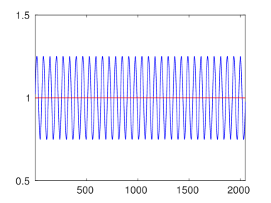
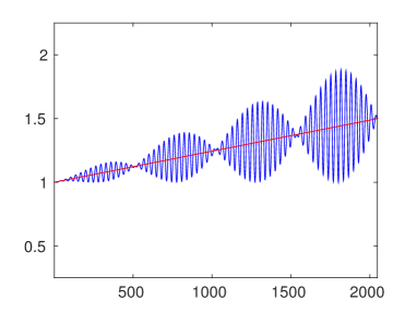
Figure 1.1. Examples of periodic and modulated periodic coefficients in 1D.

Figure 1.1 (1D case) represents examples of highly oscillating (left) and modulated periodic coefficients (right) functions.

Figure 1.2 (2D case) illustrates the well separable equation coefficient obtained by a sum of step-type and uniformly oscillating functions.

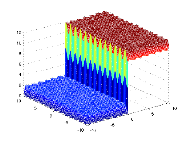
Figure 1.2. An example of modulated piecewise periodic coefficients in 2D.

We show that specially constructed FEM type approximations of PDEs with slightly perturbed or regularly modulated periodic coefficients on $d$-fold $\underbrace{n\times\cdots\times n}$ tensor grids in $\mathbb{R}^{d}$ may lead to the discretized algebraic equations with the low Kronecker rank stiffness matrix of size $n^{d}\times n^{d}$, where $n=O(\frac{1}{\epsilon})$ is proportional to the large frequency parameter $1/\epsilon$. In this case the rank decomposition with respect to the $d$ spacial variables is applied, such that the discrete solution can be calculated in the low-rank separable form, which requires the only $O(dn)$ storage size instead of $O(n^{d})=O(\frac{1}{\epsilon^{d}})$ complexity representations which are mandatory for the traditional FEM techniques (the latter quickly leads to the bottleneck in case of small parameter $\epsilon>0$).

The arising linear system of equations can be solved by preconditioned iteration with the simple preconditioner $\Lambda_{\circ}$, such that the storage and numerical costs scale almost linearly in the univariate discrete problem size $n$, i.e., they are estimated by

$$O(dn\log^{p}(\frac{1}{\epsilon}))\ll O(\frac{1}{\epsilon^{d}}),\quad p>0,$$

where $d$ is the spatial dimension. Numerical examples in Section 5 demonstrate the stable geometric convergence of the preconditioned CG (PCG) iteration with the preconditioner $\Lambda_{\circ}$ and confirm the the low-rank approximate separable representation to the solution with respect to $d$ spacial variables even in the case of complicated quasi-periodic coefficients.

This approach is well suited for applying the quantized-TT (QTT) tensor approximation [20] to functions discretized on large tensor grids of size proportional to the frequency parameter, i.e. $n=O(1/\epsilon)$, as it was demonstrated in the previous paper [23] for the case $d=1$. The use of tensor-structured preconditioned iteration with the adaptive QTT rank truncation may lead to the logarithmic complexity in the grid size, $O(\log^{p}n)$, see [19, 21, 26] for the rank-truncated iterative methods, [15, 16, 14, 13] for various examples of the QTT tensor approximation to lattice structured systems, and [2] for tensor approximation of complicated functions with multiple cusps in $\mathbb{R}^{d}$.

In Section 6, we conclude with the discussion on further perspectives of the presented approach for 2D and 3D elliptic PDEs with quasi periodic coefficients.

2. The iteration method

Let $v\in V$ and $\rho\in{\mathbb{R}}_{+}$. Consider the problem: find $u_{v}$ such that

(2.1) $$(\Lambda_{\circ}Qu_{v},Qw)=\ell^{\circ}_{v}(w)-\rho\,\ell_{v}(w)\qquad\forall w\in V,$$

where

$$\ell_{v}(w):=(\Lambda Qv,Qw)-<f,w>\quad{\rm and}\quad\ell^{\circ}_{v}(w):=(\Lambda_{\circ}Qv,Qw).$$

Obviously, the right hand side of (2.1) is a bounded linear functional on $V$, so that this problem has a unique solution $u_{v}$. Thus, we have a mapping $T_{\rho}:V\rightarrow V$, which becomes a contraction if the parameter $\rho$ is properly selected. Indeed, for any $v_{1}$ and $v_{2}$ in $V$, we obtain

(2.2) $$(\Lambda_{\circ}Q\eta,Qw)=(\Lambda_{\circ}Q\zeta-\rho\Lambda Q\zeta,Qw))\qquad\forall w\in V,$$

where $u_{1}=T_{\rho}v_{1}$, $u_{2}=T_{\rho}v_{2}$, $\zeta:=v_{1}-v_{2}$, and $\eta:=u_{1}-u_{2}$. Hence

(2.3) $$\|\eta\|^{2}_{\circ}:=(\Lambda_{\circ}Q\eta,Q\eta)=(\Lambda_{\circ}Q\zeta,Q\eta)-\rho(\Lambda Q\zeta,Q\eta)\\ =(Q\zeta,\Lambda_{\circ}Q\eta)-\rho(\Lambda^{-1}_{\circ}\Lambda Q\zeta,\Lambda_{\circ}Q\eta)=(Q\zeta-\rho\Lambda^{-1}_{\circ}\Lambda Q\zeta,\Lambda_{\circ}Q\eta)\\ \leq\|\eta\|_{\circ}\left(\Lambda_{\circ}Q\zeta-\rho\,\Lambda Q\zeta,Q\zeta-\rho\,\Lambda^{-1}_{\circ}\Lambda Q\zeta\right)^{1/2}.$$

¿From (2.3) we find that

(2.4) $$\|\eta\|^{2}_{\circ}\leq\,(\Lambda_{\circ}Q\zeta,Q\zeta)-2\rho(\Lambda Q\zeta,Q\zeta)+\rho^{2}(\Lambda^{-1}_{\circ}\Lambda Q\zeta,\Lambda Q\zeta)\\ =(Q\zeta,\Lambda_{\circ}Q\zeta)-2\rho(\Lambda^{-1}_{\circ}\Lambda Q\zeta,\Lambda_{\circ}Q\zeta)+\rho^{2}(\Lambda^{-1}_{\circ}\Lambda\Lambda^{-1}_{\circ}\Lambda Q\zeta,\Lambda_{\circ}Q\zeta)\\ =(({\mathbb{I}}-2\rho\Lambda^{-1}_{\circ}\Lambda+\rho^{2}\Lambda^{-1}_{\circ}\Lambda\Lambda^{-1}_{\circ}\Lambda)Q\zeta,\Lambda_{\circ}Q\zeta)=(\Lambda_{\circ}{\mathbb{B}}^{2}_{\rho}Q\zeta,Q\zeta)\\ \leq(\Lambda_{\circ}{\mathbb{B}}^{2}_{\rho}Q\zeta,{\mathbb{B}}^{2}_{\rho}Q\zeta)^{1/2}(\Lambda_{\circ}Q\zeta,Q\zeta)^{1/2},$$

where ${\mathbb{B}}_{\rho}$ is defined by (1.2). If $\rho$ is selected such that

(2.5) $$(\Lambda_{\circ}{\mathbb{B}}^{2}_{\rho}Q\zeta,Q\zeta)\,\leq\,q^{2}\|\zeta\|^{2}_{\circ},\qquad{\rm for\;some}\;q<1,$$

then (2.4) shows that $T_{\rho}$ is a contractive mapping.

It is not difficult to show that $\rho$ satisfying (2.5) can be always found. Indeed, in view of (1.5)

(2.6) $$(\Lambda_{\circ}{\mathbb{B}}^{2}_{\rho}Q\zeta,Q\zeta)=(\Lambda_{\circ}Q\zeta,Q\zeta)-2\rho(\Lambda Q\zeta,Q\zeta)+\rho^{2}(\Lambda\Lambda^{-1}_{\circ}\Lambda Q\zeta,Q\zeta)\\ \leq(1-2\rho c_{1})(\Lambda_{\circ}Q\zeta,Q\zeta)+\rho^{2}(\Lambda^{-1}_{\circ}\Lambda Q\zeta,\Lambda Q\zeta).$$

Since $\Lambda$ and $\Lambda_{\circ}$ are invertible with trivial kernels, $\mu$ and $y_{\mu}$ are an eigenvalue and the respective eigenfunction of $\Lambda y_{\mu}=\mu\Lambda_{\circ}y_{\mu}$ if and only if they are an eigenvalue and the eigenfunction of the problem $\Lambda\Lambda^{-1}_{\circ}\Lambda y_{\mu}=\mu\Lambda y_{\mu}$. This means that

$$c_{1}(\Lambda y,y)\,\leq\,(\Lambda\Lambda^{-1}_{\circ}\Lambda y,y)\,\leq\,c_{2}(\Lambda y,y)\,\leq\,c^{2}_{2}(\Lambda_{\circ}y,y).$$

Hence

$$(\Lambda^{-1}_{\circ}\Lambda Q\zeta,\Lambda Q\zeta)\leq c^{2}_{2}\|\zeta\|^{2}_{\circ}$$

and (2.6) implies

(2.7) $$(\Lambda_{\circ}{\mathbb{B}}^{2}_{\rho}Q\zeta,Q\zeta)\,\leq\,\left(1-2\rho c_{1}+\rho^{2}c^{2}_{2}\right)\|\zeta\|^{2}_{\circ}.$$

Minimum of the expression in round brackets is attained if $\rho=\rho_{*}:=\frac{c_{1}}{c^{2}_{2}}$. For $\rho=\rho_{*}$, we find that

(2.8) $$q^{2}_{*}:=1-\frac{c^{2}_{1}}{c^{2}_{2}}\,\leq\,\hat{q}^{2}:=1-\frac{{\lambda}_{\ominus}^{2}{{\lambda}^{\circ}_{\ominus}\!}^{2}}{{\lambda}_{\oplus}^{2}{{\lambda}^{\circ}_{\oplus}\!}^{2}}\in\,[0,1).$$

Hence, $T_{\rho}$ is a contractive mapping with explicitly known contraction factor $q_{*}$. Well known results in the theory of fixed points (e.g., see [37]) yield the following result.

Theorem 2.1.

For any $u_{0}\in V$ and $\rho=\rho^{*}$ the sequence $\{u_{k}\}\in V$ of functions satisfying the relation

(2.9) $$(\Lambda_{\circ}Qu_{k},Qw)=(\Lambda_{\circ}Qu_{k-1},Qw)-\rho\Bigl{(}(\Lambda Qu_{k-1},Qw)-<f,w>\Bigr{)}\qquad\forall w\in V$$

converges to $u$ in $V$ and $\|u_{k}-u\|_{\circ}\leq q^{k}_{*}\|u_{0}-u\|_{\circ}$ as $k\rightarrow+\infty$.

Remark 2.2.

¿From (2.4) we obtain

$$\|\eta\|^{2}_{\circ}\leq\frac{1}{\lambda_{0,{\rm min}}}\|{\mathbb{B}}^{2}_{\rho}Q\zeta\|\|\zeta\|_{\circ}\leq\frac{\|{\mathbb{B}}^{2}_{\rho}\|}{\lambda^{2}_{0,{\rm min}}}\|\zeta\|^{2}_{\circ}.$$

This relation yields a simple (but not very sharp) estimate of the contraction factor.

For further analysis, it is convenient to estimate the right hand side of (2.4) by a different method. Let ${\boldsymbol{|}\!\!|}{\mathbb{B}}_{\rho}{\boldsymbol{|}\!\!|}_{\circ}$ denote the operator norm

(2.10) $${\boldsymbol{|}\!\!|}{\mathbb{B}}_{\rho}{\boldsymbol{|}\!\!|}_{\circ}:=\sup\limits_{y\in Y}\frac{\|{\mathbb{B}}_{\rho}y\|_{\circ}}{\|y\|_{\circ}}.$$

Then $\|{\mathbb{B}}_{\rho}y\|_{\circ}\,\leq\,{\boldsymbol{|}\!\!|}{\mathbb{B}}_{\rho}{\boldsymbol{|}\!\!|}_{\circ}\|y\|_{\circ}$ and

$$(\Lambda_{\circ}{\mathbb{B}}^{2}_{\rho}y,y)\,\leq\,{\boldsymbol{|}\!\!|}{\mathbb{B}}_{\rho}{\boldsymbol{|}\!\!|}^{2}_{\circ}\,\|y\|^{2}_{\circ}.$$

Hence, (2.4) yields the estimate

(2.11) $$\|\eta\|_{\circ}\,\leq\,{\boldsymbol{|}\!\!|}{\mathbb{B}}_{\rho}{\boldsymbol{|}\!\!|}_{\circ}\|\zeta\|_{\circ},$$

which shows that $T_{\rho}$ is a contraction provided that

(2.12) $${\boldsymbol{|}\!\!|}{\mathbb{B}}_{\rho}{\boldsymbol{|}\!\!|}_{\circ}\,<\,1.$$

In applications ${\mathbb{B}}_{\rho}$ is a self adjoint bounded operator acting in a finite dimensional space, so that verification of this condition amounts finding $\rho$ which yields the respective spectral radius of ${\mathbb{B}}_{\rho}$ (see Section 4).

3. Selection of $\Lambda_{\circ}$

In this section, we discuss how to select $\Lambda_{\circ}$ in order to minimize $q$ what is crucial for two major aspects of quantitative analysis: convergence of the iteration method and guaranteed a posteriori estimates. We assume that $V$, ${\mathcal{V}}$, and $Y$ are spaces of functions defined in a Lipschitz bounded domain $\Omega$ (namely $y(x)\in\mathbb{T}$ for a.e. $x\in\Omega$ where $\mathbb{T}$ may coincide with $\mathbb{R}$, ${\mathbb{R}}^{d}$, or ${\mathbb{M}}^{d\times d}$) and the operators $\Lambda$ and $\Lambda_{\circ}$ are generated by bounded scalar functions, matrices or tensors. In this case,

$$(\Lambda y,y):=\int\limits_{\Omega}\Lambda(x)y\odot y\,dx,\quad{\rm and}\quad(\Lambda_{\circ}y,y):=\int\limits_{\Omega}\Lambda_{\circ}(x)y\odot y\,dx,$$

where $\odot$ denotes the respective product of scalar, vector, or tensor functions. In view of (2.10) and (2.12), the value of $\rho$ should minimize the quantity $\sup\limits_{y\in Y}\frac{(\Lambda_{\circ}{\mathbb{B}}_{\rho}y,{\mathbb{B}}_{\rho}y)}{(\Lambda_{\circ}y,y)}.$ This procedure yields the contraction factor

(3.1) $$q^{2}={\mathcal{Q}}(\Lambda,\Lambda_{\circ}):=\inf\limits_{\rho}\,\sup\limits_{y\in Y}\frac{\int\limits_{\Omega}\Lambda_{\circ}(x){\mathbb{B}}_{\rho}(x)y\odot{\mathbb{B}}_{\rho}(x)y\,dx}{\int\limits_{\Omega}\Lambda_{\circ}(x)y\odot y\,dx},$$

which computation is reduced to ${\mathbb{B}}_{\rho}(x)$ to solving algebraic problems at a.e. $x\in\Omega$, i.e.,

(3.2) $${\mathcal{Q}}(\Lambda,\Lambda_{\circ}):=\inf\limits_{\rho}\,\sup\limits_{x\in\Omega}\,\sup\limits_{\tau\in{\mathbb{T}}}\frac{\Lambda_{\circ}(x){\mathbb{B}}_{\rho}(x)\tau\odot{\mathbb{B}}_{\rho}(x)\tau}{\Lambda_{\circ}(x)\tau\odot\tau}$$

Let $\mathds{S}$ be a certain set of ”simple” operators defined a priori (e.g., it can be a finite dimensional set formed by piece vise constant or polynomial functions). Then, finding the best ”simplified” operator amounts solving the problem: find $\widehat{\Lambda}_{\circ}\in\mathbb{S}$ such that ${\mathcal{Q}}(\Lambda,\widehat{\Lambda}_{\circ})$ is minimal. In other words, optimal $\widehat{\Lambda}_{\circ}$ is defined by the problem

(3.3)

$$\ \inf\limits_{\,\Lambda_{0}\in\mathds{S},\atop\rho\in\mathbb{R}}\,\sup\limits_{x\in\Omega\atop\tau\in{\mathbb{T}}}\frac{\displaystyle\Lambda_{\circ}(x){\mathbb{B}}_{\rho}(x)\tau\odot{\mathbb{B}}_{\rho}(x)\tau}{\displaystyle\Lambda_{\circ}(x)\tau\odot\tau}\,=\,q^{2}.$$

Notice that (3.3) is an algebraic problem, which should be solved (analytically or numerically) before computations. The respective solution $\widehat{\Lambda}_{\circ}$ defines the best operator to be used in the iteration method (2.9) and yields the respective contraction factor. Below we discuss some particular cases, where analysis of this problem generates optimal (or almost optimal) $\Lambda_{\circ}$.

Problem (3.3) is explicitly solvable if $\Lambda_{\circ}$ and $\Lambda$ have a special structure, namely,

$$\Lambda_{\circ}=a_{\circ}(x){\mathbb{I}},\qquad\Lambda=a(x){\mathbb{I}},$$

where ${\mathbb{I}}$ is the unit operator and $a_{\circ}(x)$ and $a(x)$ are positive bounded functions defined in $\Omega$. Then,

$${\mathbb{B}}_{\rho}(x)=(1-{\mathds{h}}(x)){\mathbb{I}},\qquad{\mathds{h}}(x):=\frac{a(x)}{a_{\circ}(x)}$$

and

$$\sup\limits_{\tau\in{\mathbb{T}}}\frac{\left(1-\rho{\mathds{h}}(x)\right)^{2}\tau\odot\tau}{|\tau|^{2}}\,=\,|1-\rho{\mathds{h}}(x)|^{2}\qquad\forall\,x\in\Omega.$$

Define ${\mathds{h}}_{\ominus}:=\min\limits_{x\in\Omega}{\mathds{h}}(x)$ and ${\mathds{h}}_{\oplus}:=\max\limits_{x\in\Omega}{\mathds{h}}(x)$. It is not difficult to show that

$$\sup\limits_{x\in\Omega}|1-\rho{\mathds{h}}(x)|=\max\{|1-\rho{\mathds{h}}_{\ominus}|,|1-\rho{\mathds{h}}_{\oplus}|\}.$$

Minimization with respect to $\rho$ yields the best value $\rho_{*}=\frac{2}{{\mathds{h}}_{\ominus}+{\mathds{h}}_{\oplus}}$ and the respective value

(3.4) $${\mathcal{Q}}(\Lambda,\Lambda_{\circ})=\left(\frac{{\mathds{h}}_{\oplus}-{\mathds{h}}_{\ominus}}{{\mathds{h}}_{\oplus}+{\mathds{h}}_{\ominus}}\right)^{2}=\left(\frac{1-{\mathcal{J}(a,a_{\circ})}}{1+{\mathcal{J}(a,a_{\circ})}}\right)^{2}<1,\qquad{\mathcal{J}(a,a_{\circ})}=\frac{{\mathds{h}}_{\ominus}}{{\mathds{h}}_{\oplus}}.$$

In accordance with (3.3) identification of the optimal simplified problem is reduced to the problem

(3.5) $$\sup\limits_{a_{0}\in{\mathbb{S}}}\;{\mathcal{J}(a,a_{\circ})}.$$

where ${\mathbb{S}}$ is a given set of functions.

We illustrate the above relations by means of several examples.
Example 1. Constant coefficients. In the simplest case, we set ${\mathbb{S}}=P^{0}$, i.e., $a_{0}$ is a constant. From (3.5) it follows that $q=\displaystyle{\frac{\overline{a}-\underline{a}}{\overline{a}+\underline{a}}}$, where $\underline{a}:=\min\limits_{x\in\Omega}{a}(x)$ and $\overline{a}:=\max\limits_{x\in\Omega}{a}(x)$. Then $\rho_{*}=\frac{2a_{0}}{\overline{a}+\underline{a}}$ and the iteration procedure (2.9) with $\rho=\rho_{*}$ has the form

(3.6) $$\int\limits_{\Omega}Qu_{k}\odot Qw\,dx=\int\limits_{\Omega}\left(1-\frac{2a}{\overline{a}+\underline{a}}\right)Qu_{k-1}\odot Qw\,dx+\frac{2}{\overline{a}+\underline{a}}\int\limits_{\Omega}fw\,dx$$

From Theorem 2.1, it follows that

$$\int\limits_{\Omega}|Q(u_{k}-u)|^{2}\,dx\,\leq C\left(\displaystyle{\frac{\overline{a}-\underline{a}}{\overline{a}+\underline{a}}}\right)^{2k}.$$

Example 2. Oscillation around a given function. Consider a somewhat different example. Let $a(x)$ be a function oscillating around a certain mean function $g(x)$ so that

$$\displaystyle\frac{a(x)}{g(x)}\in[1-\epsilon,1+\epsilon],\quad\epsilon\in(0,1).$$

If $g$ is a relatively simple function, then it is natural to set $a_{\circ}(x)=g(x)$. By (3.4), we find that ${\mathds{h}}_{\oplus}=\,1+\epsilon$, ${\mathds{h}}_{\ominus}=1-\epsilon$, and $q=\epsilon$. Hence the method is very efficient for small $\epsilon$ (i.e., if $a$ oscillates around $g$ with a relatively small amplitude). Figures 1.1 and 1.2 illustrate three examples of quasi-periodic coefficients $a$ and respective $a_{\circ}$ corresponding to the case of oscillation around constant with smooth modulation, oscillation around given smooth function, or oscillation around piecewise constant function.

Example 3. Piecewise constant coefficients. Consider a more complicated case, where $\Omega$ is divided into $N$ nonoverlapping subdomains $\Omega_{i}$ and $\Lambda_{\circ}(x)=c_{i}{\mathbb{I}}$ if $x\in\Omega_{i}$. Define the numbers $a^{(i)}_{\oplus}:=\max\limits_{x\in\Omega_{i}}a(x)$, $a^{(i)}_{\ominus}:=\min\limits_{x\in\Omega_{i}}a(x)$,

$${\mathds{h}}_{\ominus}=\min\left\{\frac{a^{(1)}_{\ominus}}{c_{1}},\frac{a^{(2)}_{\ominus}}{c_{2}},...,\frac{a^{(N)}_{\ominus}}{c_{N}}\right\},\quad{\rm and}\quad{\mathds{h}}_{\oplus}=\max\left\{\frac{a^{(1)}_{\oplus}}{c_{1}},\frac{a^{(2)}_{\oplus}}{c_{2}},...,\frac{a^{(N)}_{\oplus}}{c_{N}}\right\}.$$

Since the constantans $c_{i}$ are defined up to a common multiplier, we can without a loss of generality assume that

(3.7) $$\sum^{(N)}_{i=1}\lambda_{i}=1,\qquad{\rm where}\qquad\lambda_{i}=\frac{1}{c_{i}}.$$

In accordance with (3.5), maximum of ${\mathcal{Q}}(\Lambda,\Lambda_{\circ})$ is attained if

(3.8) $$\frac{\min\left\{\lambda_{1}a^{(1)}_{\ominus},\lambda_{2}a^{(2)}_{\ominus},...,\lambda_{N}a^{(N)}_{\ominus}\right\}}{\max\left\{\lambda_{1}a^{(1)}_{\oplus},\lambda_{2}a^{(2)}_{\oplus},...,\lambda_{N}a^{(N)}_{\oplus}\right\}}\,\rightarrow\,max,$$

where $\lambda_{i}>0$ and satisfy (3.7). If $N=2$, then the problem (3.8) has a simple solution, which shows that the ratio $\frac{\lambda_{1}}{\lambda_{2}}$ (i.e., $\frac{c_{2}}{c_{1}}$) can be any in the interval $[\xi_{1},\xi_{2}]$, where $\xi_{1}=\min\{\frac{a^{(2)}_{\ominus}}{a^{(1)}_{\ominus}},\frac{a^{(2)}_{\oplus}}{a^{(1)}_{\oplus}}\}$ and $\xi_{2}=\max\{\frac{a^{(2)}_{\ominus}}{a^{(1)}_{\ominus}},\frac{a^{(2)}_{\oplus}}{a^{(1)}_{\oplus}}\}$.

It is interesting to compare these results with those generated by homogenized models in the case of perfectly periodic structures. For this purpose, we consider a simple $1$-dimensional problem

$$(au^{\prime})^{\prime}-f=0\qquad{\rm in}\;(0,1)$$

with

$$a(x)=a^{(1)}(x)\qquad{\rm in}\;\Omega_{1}=(0,\beta),\qquad\beta\in(0,1),$$

$$a(x)=a^{(2)}(x)\qquad{\rm in}\;\Omega_{2}=(\beta,1),$$

where $a^{(1)}(x)$ is a perfectly periodical function attaining only two values $a^{(1)}_{\oplus}$ (Lebesgue measure of this set is $\kappa_{1}|\Omega_{1}|$, $\kappa_{1}\in(0,1)$) and $a^{(1)}_{\ominus}$ (Lebesgue measure of this set is $(1-\kappa_{1})|\Omega_{1}|$). Similarly, $a^{(2)}(x)$ is a perfectly periodical function attaining only two values $a^{(2)}_{\oplus}$ (Lebesgue measure of this set is $\kappa_{2}|\Omega_{2}|$, $\kappa_{2}\in(0,1)$) and $a^{(2)}_{\ominus}$ (Lebesgue measure of this set is $(1-\kappa_{2})|\Omega_{2}|$). Assume that the amount of periods is very large and, therefore, the homogenization method can be successfully applied. The corresponding homogenized problem has the following coefficients

$$\widehat{a}^{(1)}:=\left(\frac{1}{\beta}\int\limits^{\beta}_{0}\frac{1}{a^{(1)}(x)}\,dx\right)^{-1}\quad{\rm in}\;\Omega_{1}\quad{\rm and}\quad\widehat{a}^{(2)}:=\left(\frac{1}{1-\beta}\int\limits^{1}_{\beta}\frac{1}{a^{(2)}(x)}\,dx\right)^{-1}\quad{\rm in}\;\Omega_{2}.$$

It is easy to see that

$$\widehat{a}^{(1)}=\frac{a^{(1)}_{\ominus}a^{(1)}_{\oplus}}{\kappa_{1}a^{(1)}_{\ominus}+(1-\kappa_{1})a^{(1)}_{\oplus}}\in(a^{(1)}_{\ominus},a^{(1)}_{\oplus}),\qquad\widehat{a}^{(2)}=\frac{a^{(2)}_{\ominus}a^{(2)}_{\oplus}}{\kappa_{2}a^{(2)}_{\ominus}+(1-\kappa_{2})a^{(2)}_{\oplus}}\in(a^{(2)}_{\ominus},a^{(2)}_{\oplus})$$

Hence

$$\frac{\widehat{a}^{(2})}{\widehat{a}^{(1)}}\in(\zeta_{1},\zeta_{2}),\quad{\rm where}\quad\zeta_{1}:=\frac{\min\{a^{(1)}_{\ominus},a^{(2)}_{\ominus}\}}{\max\{a^{(1)}_{\ominus},a^{(2)}_{\ominus}\}},\quad\zeta_{2}:=\frac{\max\{a^{(1)}_{\ominus},a^{(2)}_{\ominus}\}}{\min\{a^{(1)}_{\ominus},a^{(2)}_{\ominus}\}}.$$

It is clear that $\zeta_{1}\leq\xi_{1}$ and $\zeta_{2}\geq\xi_{2}$. Therefore, homogenized coefficients may not generate the best piece wise constant $a_{\circ}$, which produces the smallest contraction factor $q$.

4. Error estimates

4.1. General estimate

Since $T_{\rho}$ is a contractive mapping, we can use the Ostrowski estimates (see [30, 37, 32]), which yield the estimate of the distance between $v\in V$ and the fixed point:

(4.1) $$\|v-u\|_{\circ}\,\in\left\{\frac{\epsilon}{1+q(\rho)},\,\frac{\epsilon}{1-q(\rho)}\right\},\qquad{\rm where}\;\epsilon:=\|T_{\rho}v-v\|_{\circ}.$$

The is estimate cannot be directly applied because $v_{\rho}:=T_{\rho}v$ is generally unknown (it is the exact solution of a boundary value problem). Instead, we must use a numerical approximation $\widetilde{v}_{\rho}$ (in our analysis, we impose no restrictions on the method by which the function $\widetilde{v}_{\rho}\in V$ was constructed). Thus, the difference $\eta_{\rho}:=v-\widetilde{v}_{\rho}$ is a known function and the quantity $\delta_{\rho}=\|\eta_{\rho}\|_{\circ}$ is directly computable. It is easy to see that

(4.2) $$\delta_{\rho}-\|\widetilde{v}_{\rho}-v_{\rho}\|_{\circ}\,\leq\,\|v_{\rho}-v\|_{\circ}\,\leq\,\delta_{\rho}+\|\widetilde{v}_{\rho}-v_{\rho}\|_{\circ}.$$

To deduce a fully computable majorant of the norm $\|\widetilde{v}_{\rho}-v_{\rho}\|_{\circ}$ we use the method suggested in [31, 32]. First, we rewrite (2.1) in the form

(4.3) $$(\Lambda_{\circ}Qv_{\rho},Qw)=(\Lambda_{\circ}Qv,Qw)-\rho\Bigl{(}(\Lambda Qv,Qw)-<f,w>\Bigr{)}.$$

For any $y\in Y$ and $w\in V_{0}$, we have

$$(\Lambda_{\circ}Q(v_{\rho}-\widetilde{v}_{\rho}),Qw) =(\Lambda_{\circ}Q(v-\widetilde{v}_{\rho}),Qw))-\rho\,\Bigl{(}(\Lambda Qv,Qw)-<f,w>\Bigr{)}$$

$$=(\Lambda_{\circ}Q(v-\widetilde{v}_{\rho})-\rho\Lambda Qv+y,Qw))-<Q^{*}y+\rho f,w>.$$

We estimate the first term in the right hand side of (4.1) as follows:

$$(\Lambda_{\circ}Q(v-\widetilde{v}_{\rho})-\rho\Lambda Qv+y,Q(v_{\rho}-\widetilde{v}_{\rho})))=(Q(v-\widetilde{v}_{\rho})-\rho\Lambda^{-1}_{\circ}\Lambda Qv+\Lambda^{-1}_{\circ}y,\Lambda_{\circ}Q(v_{\rho}-\widetilde{v}_{\rho})))\\ \leq\left(\Lambda_{\circ}Q(v-\widetilde{v}_{\rho})+\tau,Q(v-\widetilde{v}_{\rho})+\Lambda^{-1}_{\circ}\tau\right)^{1/2}\|v_{\rho}-\widetilde{v}_{\rho}\|_{\circ},$$

where $\tau:=y-\rho\Lambda Qv$. The second term meets the estimate

$$<Q^{*}y+f,v_{\rho}-\widetilde{v}_{\rho}>\,\leq\,{\boldsymbol{|}\!\!|}Q^{*}y+\rho f{\boldsymbol{|}\!\!|}\,\|v_{\rho}-\widetilde{v}_{\rho}\|\,\leq\,\frac{1}{({\lambda}^{\circ}_{\ominus})^{1/2}}{\boldsymbol{|}\!\!|}Q^{*}y+\rho f{\boldsymbol{|}\!\!|}\,\|v_{\rho}-\widetilde{v}_{\rho}\|_{\circ},$$

where ${\boldsymbol{|}\!\!|}w^{*}{\boldsymbol{|}\!\!|}\,=\,\sup\limits_{w\in V}\frac{<w^{*},w>}{\|w\|_{\circ}}$ is the dual norm. Hence,

(4.5) $$\|v_{\rho}-\widetilde{v}_{\rho}\|_{\circ}\,\leq\,\left(\Lambda_{\circ}Q\eta_{\rho}+\tau,Q\eta_{\rho}+\Lambda^{-1}_{\circ}\tau\right)^{1/2}+\frac{1}{\sqrt{{\lambda}^{\circ}_{\ominus}}}{\boldsymbol{|}\!\!|}Q^{*}y+\rho f{\boldsymbol{|}\!\!|}=:M_{\oplus}(\eta_{\rho},\tau).$$

Notice that

$$\inf\limits_{y\in Y}M_{\oplus}(\eta_{\rho},\tau)=\|v_{\rho}-\widetilde{v}_{\rho}\|_{\circ}.$$

Indeed, set $y=\Lambda_{\circ}Q(v_{\rho}-v)+\rho\Lambda Qv$. Then, $\tau=\Lambda_{\circ}Q(v_{\rho}-v)$. In view of (4.3), $Q^{*}y+\rho f=0$, and the majorant is equal to $\|v_{\rho}-\widetilde{v}_{\rho}\|^{2}_{\circ}$. Hence, the estimate (4.5) has no gap.

It is worth noting that computation of the majorant $M_{\oplus}$ does not require inversion of the operator $\Lambda$ associated with a complicated quasi–periodic problem.

Remark 4.1.

$M_{\oplus}(\eta_{\rho},\tau)$ is an a posteriori error majorant of the functional type (its derivation is performed by purely functional methods based on generalized formulation of the boundary value problem and special properties of approximations or numerical method are not used). Properties of such type error majorants are well studied (see [31, 32] and the literature cited therein). It is not difficult to show that the last term of $M_{\oplus}(\eta_{\rho},\tau)$ can be estimated via an explicitly computable quantity provided that $y$ has the same regularity as the true flux. However, in our subsequent analysis these advanced forms of the majorant are not required. Therefore we omit this discussion (interested reader can find the respective analysis in [32]). Numerous tests performed for different boundary value problems have confirmed high practical efficiency of error majorants of the functional type. It was shown that $M_{\oplus}$ is a guaranteed and efficient majorant of the global error and generates good indicators of local errors if $y$ is replaced by a certain numerical reconstruction of the exact dual solution. There are many different ways to obtain suitable reconstructions (see [27] for a systematic discussion of computational aspects of this error estimation method). Error majorants of this type can be also used for the evaluation of modeling errors (see [35, 34]).

Now, (4.1), (4.2), and (4.5) yield the following result

Theorem 4.2.

The error $e=v-u$ is subject to the estimate

(4.6) $$\|e\|_{\circ}\,\in\left[\;\max\left\{0,\,\frac{\delta_{\rho}-M_{\oplus}(\eta_{\rho},\tau)}{1+q(\rho)}\right\},\;\frac{\delta_{\rho}+M_{\oplus}(\eta_{\rho},\tau)}{1-q(\rho)}\;\right],$$

where $\tau:=y-\rho\Lambda Qv$ and $y$ is a function in $Y$ and $M_{\oplus}$ is defied by (4.5).

If $Q^{*}y+\rho f=0$ then $M^{2}_{\oplus}(\eta_{\rho},\tau)=(\Lambda_{\circ}Q\eta_{\rho},Q\eta_{\rho})+(\Lambda_{\circ}^{-1}\tau,\tau)-2(Q\eta_{\rho},\tau).$

4.2. Examples

Now we shortly discuss applications of Theorem 4.2 to problems, where $Q$ and $Q^{*}$ are defined by the operators $\nabla$ and ${\rm div}$, respectively, $\Lambda_{\circ}=a_{\circ}(x){\mathbb{I}}$, $\Lambda=a(x){\mathbb{I}}$, $x\in\Omega$, and $V=\stackrel{{\scriptstyle\circ}}{{H}}\!{}^{1}(\Omega)$.

4.2.1. $d=1$

Let $\Omega=(0,1)$. The equation (1.1) has the form $(a(x)u^{\prime})^{\prime}-f=0$. In this case, $Qw=w^{\prime}$, $Q^{*}y=-y^{\prime}$, and (4.3) is reduced to

(4.7) $$\int\limits^{1}_{0}a_{\circ}(v_{\rho}-v)^{\prime}w^{\prime}\,dx+\rho\int\limits^{1}_{0}(av^{\prime}w^{\prime}+fw)\,dx=0.$$

In order to apply Theorem 4.2, we set $y=\rho(g(x)+\mu)$, where $g(x)=-\int^{x}_{0}fdx$ and $\mu$ is a constant. Then $-y^{\prime}-\rho f=0$ and $\tau=\rho(g(x)+\mu)-\rho av^{\prime}=\rho(\mu+g-av^{\prime})$. The best constant $\mu$ is defined by minimization of $M^{2}_{\oplus}(\eta_{\rho},\tau)$, which has the form

$$\int\limits^{1}_{0}(a_{\circ}(\eta^{\prime}_{\rho})^{2}+a_{\circ}^{-1}\rho^{2}(\mu+g-av^{\prime})^{2}-2\eta^{\prime}_{\rho}\rho(\mu+g-av^{\prime})dx$$

Since $\int^{1}_{0}\eta^{\prime}_{\rho}dx=0$, the problem is reduced to minimization of the second term and the best $\mu$ satisfies the equation $\int\limits^{1}_{0}a^{-1}_{\circ}(\mu+g(x)-av^{\prime})dx=0.$ Hence

$$\mu=\bar{\mu}:=\frac{\int^{1}_{0}a^{-1}_{\circ}(av^{\prime}-g)dx}{\int^{1}_{0}a^{-1}_{\circ}\,dx},$$

and (4.6) yields the estimate

(4.8) $$\|e\|_{\circ}\,\in\left[\;\max\left\{0,\,\frac{\delta_{\rho}-I_{\oplus}(v,\widetilde{v}_{\rho})}{1+q(\rho)}\right\},\;\frac{\delta_{\rho}+I_{\oplus}(v,\widetilde{v}_{\rho})}{1-q(\rho)}\right],$$

where

$$I^{2}_{\oplus}(v,\widetilde{v}_{\rho})=\int\limits^{1}_{0}a^{-1}_{\circ}\Bigl{(}a_{\circ}(v-\widetilde{v}_{\rho})^{\prime}-\rho(\bar{\mu}+g-av^{\prime})\Bigr{)}^{2}dx.$$

Here $v$ and $\widetilde{v}_{\rho}$ are two consequent numerical approximations (e.g., finite element approximations $v^{k}_{h}$ and $v^{k+1}_{h}$ computed on a mesh ${\mathcal{I}}_{h}$. Then

$$\eta_{\rho}=\eta^{k}_{h}:=v^{k}_{h}-v^{k+1}_{h}\;{\rm and}\;\delta_{\rho}=\delta^{k}:=\|v^{k}_{h}-v^{k+1}_{h}\|_{\circ}$$

are directly computable. Since $a_{\circ}$ is a ”simple” function, the integrals

$$F_{1}=\int^{1}_{0}\!\!\!a^{-1}_{\circ}\,dx,\;F_{2}=\int^{1}_{0}\!\!\!a^{-1}_{\circ}\,g\,dx,\;F_{3}=\int^{1}_{0}\!\!\!a_{\circ}\left(\eta^{k\,\prime}_{h}\right)^{2}\,dx,\;F_{4}=\int^{1}_{0}\!\!\!a_{\circ}\left(\bar{\mu}+g\right)^{2}\,dx,\;F_{5}=\int^{1}_{0}\!\!\!f\eta^{k}_{h}\,dx$$

are easy to compute. Other integrals

$$G_{1}=\int^{1}_{0}\!\!\!a^{-1}_{\circ}a\,v^{k\,\prime}_{h}\,dx,\;G_{2}=\int^{1}_{0}\!\!\!a\,(v^{k}_{h})^{\prime}\,\eta^{k\,\prime}_{h}\,dx,\;G_{3}=\int^{1}_{0}\!\!\!(\bar{\mu}+g)a^{-1}_{\circ}a\,v^{k\,\prime}_{h}\,dx,\;G_{4}=\int^{1}_{0}\!\!\!a^{-1}_{\circ}\,a^{2}\,\left(v^{k\,\prime}_{h})\right)^{2}\,dx$$

contain highly oscillating coefficient $a$ multiplied by piece wise polynomial mesh functions. If $a$ has a low QTT rank tensor representation [20], then the integrals can be efficiently computed by tensor type methods already discussed in [23]. We have

$$I^{2}_{\oplus}(v,\widetilde{v}_{\rho})=F_{3}+2G_{2}+2\rho F_{5}+\rho^{2}(F_{4}-2G_{3}+G_{4})=:\varepsilon^{k},\qquad\bar{\mu}=\frac{G_{1}-F_{2}}{F_{1}}.$$

Here $\rho=\frac{2}{{\mathds{h}}_{\ominus}+{\mathds{h}}_{\oplus}}$ is selected in accordance with Section 3. The respective contraction factor is $q=\frac{{\mathds{h}}_{\oplus}-{\mathds{h}}_{\ominus}}{{\mathds{h}}_{\ominus}+{\mathds{h}}_{\oplus}}$. Now (4.8) yields easily computable lower and upper bounds of the error encompassed in $v^{k}_{h}$:

$$\frac{\delta^{k}-\varepsilon^{k}}{1+q}\,\leq\,\|v^{k}_{h}-u\|_{\circ}\,\leq\,\frac{\delta^{k}+\varepsilon^{k}}{1-q}$$

4.2.2. $d=2$

Computation of $M_{\oplus}$ for 2d problems can be also reduced to the computation of one dimensional integrals. Certainly on the multidimensional case the amount of integrals is much larger. However the basic tensor decomposition methods remain the same. Below we briefly discuss them with the paradigm of a simple case where

$$f=f^{(1)}(x_{1})f^{(2)}(x_{2})\quad{\rm and}\quad a=a^{(1)}(x_{1})a^{(2)}(x_{2}).$$

Assume that approximations are represented in the form of series formed by one dimensional functions $\phi^{(1)}_{i}$ and $\phi^{(2)}_{j}$ (which may be supported locally or globally), so that

$$v=\sum\limits^{n_{1}}_{i=1}\sum\limits^{n_{2}}_{j=1}\gamma_{ij}\phi^{(1)}_{i}(x_{1})\phi^{(2)}_{j}(x_{2}),\quad\widetilde{v}_{\rho}=\sum\limits^{n_{1}}_{i=1}\sum\limits^{n_{2}}_{j=1}\widetilde{\gamma}_{ij}\phi^{(1)}_{i}(x_{1})\phi^{(2)}_{j}(x_{2}).$$

In this case,

$$\nabla\eta_{\rho}=\left(\sum\limits^{n_{1}}_{i=1}\sum\limits^{n_{2}}_{j=1}\varsigma_{ij}\frac{\partial\phi^{(1)}_{i}}{\partial x_{1}}\phi^{(2)}_{j}\,,\,\sum\limits^{n_{1}}_{i=1}\sum\limits^{n_{2}}_{j=1}\varsigma_{ij}\phi^{(1)}_{i}\frac{\partial\phi^{(2)}_{j}}{\partial x_{2}}\right),\quad{\rm where}\quad\varsigma_{ij}=\gamma_{ij}-\widetilde{\gamma}_{ij}.$$

We define another set of one dimensional functions $W^{(1)}_{k}(x_{1})$ and $W^{(2)}_{l}(x_{2})$, which form the vector function

(4.9) $$y=\Upsilon_{0}+\sum\limits^{m_{1}}_{k=1}\sum\limits^{m_{2}}_{l=1}\sigma_{kl}\Upsilon_{kl},\quad\Upsilon_{kl}=\left\{W^{(1)}_{k}\frac{\partial W^{(2)}_{l}}{\partial x_{2}}\;;\;-\frac{\partial W^{(1)}_{k}}{\partial x_{1}}W^{(2)}_{l}\right\}.$$

Here $\Upsilon_{0}$ is a given function, which can be defined in different ways. In particular, we set $\Upsilon_{0}=\left\{W^{(1)}_{0}(x_{1})W^{(2)}_{0}(x_{2})\,;\,0\right\}$, $W^{(1)}_{0}(x_{1})=\int^{x_{1}}_{0}f^{(1)}dx_{1}$ and $W^{(2)}_{0}=-\rho f^{(2)}$. The functions $\Upsilon_{kl}$ must satisfy the usual linear independence conditions in order to guarantee unique solvability of the respective approximation problem. For any smooth function $w$ vanishing on $\partial\Omega$, we have

$$\int\limits_{\Omega}(\Upsilon_{0}\cdot\nabla w-\rho fw)dx_{1}dx_{2}=0\quad{\rm and}\quad\int\limits_{\Omega}\Upsilon_{kl}\cdot\nabla wdx_{1}dx_{2}=0.$$

Thus, ${\boldsymbol{|}\!\!|}Q^{*}y+\rho f{\boldsymbol{|}\!\!|}={\boldsymbol{|}\!\!|}{\rm div}y-\rho f{\boldsymbol{|}\!\!|}=0$ and we can use the simplified form of $M_{\oplus}$.

In the simplest case $\Lambda_{\circ}=a_{\circ}{\mathbb{I}}$, where $a_{\circ}$ is a constant. The best $y$ minimizes the quantity

(4.10) $$M^{2}_{\oplus}(\eta_{\rho},\tau)=\int\limits_{\Omega}a_{\circ}\nabla\eta_{\rho}\cdot\nabla\eta_{\rho}dx+\int\limits_{\Omega}a^{-1}_{\circ}y\cdot ydx+\rho^{2}\int\limits_{\Omega}a^{-1}_{\circ}a^{2}\nabla v\cdot\nabla vdx\\ -2\int\limits_{\Omega}(\rho a^{-1}_{\circ}a\nabla v+\nabla\eta_{\rho})\cdot y\,dx+2\rho\int\limits_{\Omega}a\nabla\eta_{\rho}\cdot\nabla\eta_{\rho}\,dx,$$

which shows that $y$ must satisfy the relation $y=\rho a\nabla v+a_{\circ}\nabla\eta_{\rho}$. We select $\sigma_{kl}$ that defines Galerkin approximation of this function and arrive at the system

(4.11) $$\sum\limits^{m_{1}}_{k=1}\sum\limits^{m_{2}}_{l=1}\sigma_{kl}\int\limits_{\Omega}\Upsilon_{kl}\cdot\Upsilon_{st}dx_{1}dx_{2}+\int\limits_{\Omega}\Upsilon_{0}\cdot\Upsilon_{st}dx_{1}dx_{2}\\ =\sum\limits^{n_{1}}_{i=1}\sum\limits^{n_{2}}_{j=1}\int\limits_{\Omega}(\rho a\gamma_{ij}+a_{\circ}\varsigma_{ij})\left(\frac{\partial\phi^{(1)}_{i}}{\partial x_{1}}\phi^{(2)}_{j},\phi^{(1)}_{i}\frac{\partial\phi^{(2)}_{j}}{\partial x_{2}}\right)\cdot\Upsilon_{st}dx_{1}dx_{2}$$

Introduce the following matrixes

$${\rm D}^{(1)}=\left\{D^{(1)}_{kl}\right\},\quad D^{(1)}_{kl}=\displaystyle\int^{a}_{0}\frac{\partial W^{(1)}_{k}}{\partial x_{1}}\frac{\partial W^{(1)}_{l}}{\partial x_{1}}dx_{1},\quad {\rm W}^{(1)}=\left\{W^{(1)}_{kl}\right\},\;W^{(1)}_{kl}=\int^{a}_{0}W^{(1)}_{k}W^{(1)}_{l}\,dx_{1},$$

$${\rm D}^{(2)}=\left\{D^{(2)}_{kl}\right\},\quad D^{(2)}_{kl}=\displaystyle\int^{b}_{0}\frac{\partial W^{(2)}_{k}}{\partial x_{2}}\frac{\partial W^{(2)}_{l}}{\partial x_{2}}dx_{2},\quad {\rm W}^{(2)}=\left\{W^{(2)}_{kl}\right\},\quad W^{(2)}_{kl}=\int^{b}_{0}W^{(2)}_{k}W^{(2)}_{l}\,dx_{2},$$

$${\rm F}^{(1)}=\left\{F^{(1)}_{ik}\right\},\quad F^{(1)}_{ik}=\displaystyle\int^{a}_{0}\frac{\partial\phi^{(1)}_{i}}{\partial x_{1}}W^{(1)}_{k}dx_{1},\quad {\rm G}^{(1)}=\left\{G^{(1)}_{ik}\right\},\quad G^{(1)}_{ik}=\int\limits^{a}_{0}\phi^{(1)}_{i}\frac{\partial W^{(1)}_{k}}{\partial x_{1}}\,dx_{1},$$

$${\rm F}^{(2)}=\left\{F^{(2)}_{jl}\right\},\quad F^{(2)}_{jl}=\displaystyle\int^{b}_{0}\phi^{(2)}_{j}\frac{\partial W^{(2)}_{l}}{\partial x_{2}}dx_{2},\quad {\rm G}^{(2)}=\left\{G^{(2)}_{jl}\right\},\quad G^{(2)}_{jl}=\int\limits^{b}_{0}\frac{\partial\phi^{(2)}_{j}}{\partial x_{2}}W^{(1)}_{l}\,dx_{2},$$

$$\widehat{\rm F}^{(1)}=\left\{\widehat{F}^{(1)}_{ik}\right\},\;\widehat{F}^{(1)}_{ik}=\displaystyle\int^{a}_{0}a_{1}(x_{1})\frac{\partial\phi^{(1)}_{i}}{\partial x_{1}}W^{(1)}_{k}dx_{1},\; \widehat{\rm G}^{(1)}=\left\{\widehat{G}^{(1)}_{ik}\right\},\;\widehat{G}^{(1)}_{ik}=\int^{a}_{0}a_{1}(x_{1})\phi^{(1)}_{i}\frac{\partial W^{(1)}_{k}}{\partial x_{1}}\,dx_{1},$$

$$\widehat{\rm F}^{(2)}=\left\{\widehat{F}^{(2)}_{jl}\right\},\;\widehat{F}^{(2)}_{jl}=\displaystyle\int^{b}_{0}a_{2}(x_{2})\phi^{(2)}_{j}\frac{\partial W^{(2)}_{l}}{\partial x_{2}}dx_{2},\; \widehat{\rm G}^{(2)}=\left\{\widehat{G}^{(2)}_{jl}\right\},\;\widehat{G}^{(2)}_{jl}=\int^{b}_{0}a_{2}(x_{2})\frac{\partial\phi^{(2)}_{j}}{\partial x_{2}}W^{(1)}_{l}\,dx_{2}.$$

and vectors

$$\boldsymbol{g}^{(1)}=\{g^{(1)}_{k}\},\quad g^{(1)}_{k}=\displaystyle\int^{a}_{0}W^{(1)}_{0}W^{(1)}_{k}\,dx_{1},\qquad\boldsymbol{g}^{(2)}=\{g^{(2)}_{l}\},\quad g^{(2)}_{l}=\displaystyle\int^{b}_{0}W^{(2)}_{0}\frac{\partial W^{(2)}_{l}}{\partial x_{2}}\,dx_{2}.$$

Notice that all coefficients are presented by one dimensional integrals, which can be efficiently computed with the help of special (tensor type) methods (see, e.g., [20]-[24]).

It is not difficult to see that

$$Y_{klst}:=\int\limits_{\Omega}\Upsilon_{kl}\cdot\Upsilon_{st}\,dx=W^{(1)}_{ks}D^{(2)}_{lt}+D^{(1)}_{ks}W^{(2)}_{lt}$$

and

$$\int\limits_{\Omega}\Upsilon_{0}\cdot\Upsilon_{st}dx_{1}dx_{2}=\int\limits_{\Omega}W^{(1)}_{0}W^{(1)}_{s}W^{(2)}_{0}\frac{\partial W^{(2)}_{t}}{\partial x_{2}}dx_{1}dx_{2}=g^{(1)}_{s}g^{(2)}_{t},$$

where ${\rm Y}=\{Y_{klst}\}$ is the fourth order tensor. Hence the left hand side of the system (4.11) has the form ${\rm Y}{\boldsymbol{\sigma}}+\boldsymbol{g}^{(1)}\otimes\boldsymbol{g}^{(2)}$. In the right hand side we have the term

$$\int\limits_{\Omega}a_{\circ}\varsigma_{ij}\left(\frac{\partial\phi^{(1)}_{i}}{\partial x_{1}}\phi^{(2)}_{j},\phi^{(1)}_{i}\frac{\partial\phi^{(2)}_{j}}{\partial x_{2}}\right)\cdot\Upsilon_{st}dx_{1}dx_{2}=a_{\circ}{\rm H}\boldsymbol{\varsigma},$$

where ${\rm H}=\{H_{ijst}\},\,H_{stij}=F^{(1)}_{is}F^{(2)}_{jt}-G^{(1)}_{is}G^{(2)}_{jt}$. Another term is

$$\int\limits_{\Omega}\rho a\gamma_{ij}\left(\frac{\partial\phi^{(1)}_{i}}{\partial x_{1}}\phi^{(2)}_{j},\phi^{(1)}_{i}\frac{\partial\phi^{(2)}_{j}}{\partial x_{2}}\right)\cdot\Upsilon_{st}dx_{1}dx_{2}=\widehat{\rm H}\boldsymbol{\gamma},$$

where $\widehat{\rm H}=\{\widehat{H}_{ijst}\},\,\widehat{H}_{stij}=\widehat{F}^{(1)}_{is}\widehat{F}^{(2)}_{jt}-\widehat{G}^{(1)}_{is}\widehat{G}^{(2)}_{jt}$.

Now (4.11) implies ${\boldsymbol{\sigma}}={\rm Y}^{-1}(\widehat{\rm H}\boldsymbol{\gamma}+a_{\circ}{\rm H}\boldsymbol{\varsigma}-\boldsymbol{g}^{(1)}\otimes\boldsymbol{g}^{(2)})$ and the value of $M_{\oplus}$ is obtained by (4.6), (4.9), and (4.10).

5. Low-rank solution of the discrete equation

In what follows we assume that $f$ and $a$ admit low rank representation (e.g., $f=\sum_{i=1}^{R_{f}}f^{i}_{1}(x_{1})f^{i}_{2}(x_{2})$, $a=\sum_{j=1}^{R_{a}}a^{j}_{1}(x_{1})a^{j}_{2}(x_{2})$). Then one may assume that the exact FEM solution can be well approximated by $u^{K}(x)=\sum^{K}_{j=1}u^{j}_{1}(x_{1})u^{j}_{2}(x_{2})$, where $K$ depends on the separation rank of $f$ and $a$. In some cases this important property can be rigorously proven (say, for Laplacian like operators). The similar low rank approximation can be observed for the QTT tensor approximation (see [23]). Existence of low rank solution means that for some $K$ we have $u_{K}\approx u$ up to the rank truncation threshold.

Here we sketch the rank-structured computational scheme. In our set of examples the original problem: find $u$ such that

(5.1) $$\int\limits_{\Omega}a(x)\nabla u\cdot\nabla w\,dx=\int\limits_{\Omega}fwdx\qquad\forall w\in V_{0}:=H^{1}_{0}$$

is replaced by the Galerkin problem for low rank representations

(5.2) $$\int\limits_{\Omega}a(x)\nabla u^{K}\cdot\nabla w^{K}\,dx=\int\limits_{\Omega}fwdx\qquad\forall w^{K}\in V^{K}_{0},$$

where $V^{K}_{0}$ is a subset of $V_{0}$ formed by functions of the type

$$w^{K}(x)=\sum^{K}_{j=1}\phi^{j}_{1}(x_{1})\phi^{j}_{2}(x_{2}).$$

Therefore, in terms of the general scheme exposed in the introduction, the Problem $\mathcal{P}$ is now the problem (5.2) and we solve it by iterations with the help of simplified (preconditioned) problem

(5.3) $$\int\limits_{\Omega}a_{\circ}(x)\nabla u_{k}\cdot\nabla w^{K}\,dx=\int\limits_{\Omega}f_{k-1}wdx\qquad\forall w^{K}\in V^{K}_{0},$$

where $a_{\circ}$ is a simple (mean) function and $f_{k-1}$ depends on $u_{k-1}$.

Given the right-hand side, the problem (5.3) is much simpler than the initial equation since the matrix $\Lambda_{\circ}$, generated by the coefficient $a_{\circ}$ is easily invertible. Moreover, the coefficient $a$ may be rather complicated and admits a representation with rank $R$, i.e.,

$$a(x)=\sum^{R}_{s=1}a^{(s)}_{1}(x_{1})...a^{(s)}_{d}(x_{d}),$$

where $R$ is a small integer. When we construct the low-rank Kronecker representation of stiffness matrix for this $a$, which is presented by elements of $4R$ matrices computed by only 1D integrals containing oscillating functions $a^{(s)}_{i}(x_{i})$.

If we use (5.3), then $a_{\circ}$ is a simple function, it may be a even a constant, or a function representable in the form $a^{\circ}_{1}(x_{1})...a^{\circ}_{d}(x_{d})$ with very simple multipliers. Then, the respective Kronecker stiffness matrix $\Lambda_{\circ}$ is computed much easier and has a simple (low rank) form that allows the low rank representation of its inverse.

5.1. Kronecker product representation of the stiffness matrix

We consider the elliptic diffusion equation with quasi-periodic coefficient $a(x)>0$ (whose oscillations are characterized by the parameter $\epsilon$)

(5.4) $${\mathcal{A}}u=-\mbox{div}(a(x)\nabla u)=f(x),\quad x=(x_{1},\ldots,x_{d})\in\Omega=(0,1)^{d},\quad{u}_{|\Gamma}=0,$$

where the function $f$ corresponds to the modified right hand side in the problem (4.3), $\Gamma=\partial\Omega$, and the right-hand side $f(x_{1},\ldots,x_{d})$ can be represented with a low separation rank.

Figure 5.1 illustrates a 2D example of $L\times L$ periodic coefficient with $L=6$ corresponding to the choice $\epsilon=1/L$.

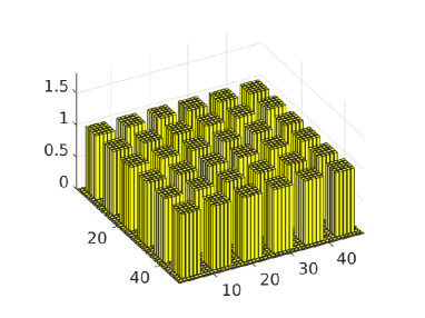
Figure 5.1. Example of the 2D periodic oscillating coefficients (left) and the 1D factor $a_{1}(x_{1})$.

In this example, the scalar coefficient is represented by the separable function $a(x)=C+a_{1}(x_{1})a_{1}(x_{2})$, $C>0$, where the generating univariate function $a_{1}(x_{1})$ has the shape of six uniformly distributed bumps of hight $1$ as shown in Figure 5.1, right. Figure 5.1, left, presents the oscillating part of 2D coefficients function, $a_{1}(x_{1})a_{1}(x_{2})$.

The examples of other possible shapes of the equation coefficient corresponding to the cases (1), (2) and (3) specified in Introduction are presented in Figures 1.1 and 1.2.

We apply the FEM Galerkin discretization of equation (5.4) by means of tensor-product piecewise affine basis functions (instead of ”linear finite elements”)

$$\{\varphi_{\bf i}(x):=\varphi_{i_{1}}(x_{1})\cdots\varphi_{i_{d}}(x_{d})\},\quad{\bf i}=(i_{1},\ldots,i_{d}),\;i_{\ell}\in{\mathcal{I}}_{\ell}=\{1,\ldots,n_{\ell}\},\;\ell=1,\ldots,d,$$

where $\varphi_{i_{k}}$ are 1D finite element basis functions (say, piecewise linear hat functions).

We associate the univariate basis functions with the uniform grid $\{\nu_{j}\}$, $j=1,\ldots,n_{\ell},$ on $[0,1]$ with the mesh size $h=1/(n_{\ell}+1)$. In this construction we have $N=n_{1}n_{2}...n_{d}$ basis functions $\varphi_{\bf i}$. Notice that the univariate grid size $n_{\ell}$ is of the order of $n_{\ell}=O(1/\epsilon)$ designating the total problem size $N=O(1/\epsilon^{d})$.

For ease of exposition we, first, consider the case $d=2$, and further assume that the scalar diffusion coefficient $a(x_{1},x_{2})$ can be represented in the form

$$a(x_{1},x_{2})=\sum\limits^{R}_{k=1}a^{(1)}_{k}(x_{1})a^{(2)}_{k}(x_{2})>0$$

with a small rank parameter $R$.

The $N\times N$ stiffness matrix is constructed by the standard mapping of the multi-index ${\bf i}$ into the $N$-long univariate index $i$ representing all degrees of freedom. For instance, we use the so-called big-endian convention for $d=3$ and $d=2$

$${\bf i}\mapsto i:=i_{3}+(i_{2}-1)n_{3}+(i_{1}-1)n_{2}n_{3},\quad{\bf i}\mapsto i:=i_{2}+(i_{1}-1)n_{2},$$

respectively. Hence all matrices and vectors are defined on the long index $i$ as usual, however, the special Kronecker structure allows the low-storage and low-complexity matrix vector multiplications when appropriate, i.e. when a vector also admits the low-rank Kronecker form representation. In particular, the basis function $\varphi_{\bf i}$ is designated via the long index, i.e. $\varphi_{i}=\varphi_{\bf i}$.

First, we consider the simplest case $R=1$ and let $d=2$. We construct the Galerkin stiffness matrix $A=[a_{ij}]\in\mathbb{R}^{N\times N}$ in the form of a sum of Kronecker products of small ”univariate” matrices. Recall that given $p_{1}\times q_{1}$ matrix $A$ and $p_{2}\times q_{2}$ matrix $B$, their Kronecker product is defined as a $p_{1}p_{2}\times q_{1}q_{2}$ matrix $C$ via the block representation

$$C=A\otimes B=[a_{ij}B],\quad i=1,\ldots,p_{1},\;j=1,\ldots,q_{1}.$$

We say that the Kronecker rank of the matrix $A$ in the representation above equals to $1$. Now the elements of Galerkin stiffness matrix take a form

(5.5) $$a_{ij}=\langle{\mathcal{A}}\varphi_{i},\varphi_{j}\rangle=\int\limits_{\Omega}a^{(1)}(x_{1})a^{(2)}(x_{2})\nabla\varphi_{i}(x)\dot{\nabla}\varphi_{j}(x)dx\\ ={\int\limits^{1}_{0}}a^{(1)}(x_{1})\frac{\partial\varphi_{i_{1}}(x_{1})}{\partial x_{1}}\frac{\partial\varphi_{j_{1}}(x_{1})}{\partial x_{1}}dx_{1}\int\limits^{1}_{0}a^{(2)}(x_{2})\varphi_{i_{2}}(x_{2})\varphi_{j_{2}}(x_{2})dx_{2}\\ +\int\limits^{1}_{0}a^{(1)}(x_{1})\varphi_{i_{1}}(x_{1})\varphi_{j_{1}}(x_{1})dx_{1}\int\limits^{1}_{0}a^{(2)}(x_{2})\frac{\partial\varphi_{i_{2}}(x_{2})}{\partial x_{2}}\frac{\partial\varphi_{j_{2}}(x_{2})}{\partial x_{2}}dx_{2},$$

which leads to the rank-2 Kronecker product representation

$${A}=[a_{ij}]={A}_{1}\otimes M_{2}+M_{1}\otimes{A}_{2},$$

where $\otimes$ denotes the conventional Kronecker product of matrices. Here ${A}_{1}=[a_{i_{1}j_{1}}]\in\mathbb{R}^{n_{1}\times n_{1}}$ and ${A}_{2}=[a_{i_{2}j_{2}}]\in\mathbb{R}^{n_{2}\times n_{2}}$ denote the univariate stiffness matrices and $M_{1}=[m_{i_{1}j_{1}}]\in\mathbb{R}^{n_{1}\times n_{1}}$ and $M_{2}=[m_{i_{2}j_{2}}]\in\mathbb{R}^{n_{2}\times n_{2}}$ define the corresponding weighted mass matrices, e.g.,

$$a_{i_{1}j_{1}}={\int\limits^{1}_{0}}a^{(1)}(x_{1})\frac{\partial\varphi_{i_{1}}(x_{1})}{\partial x_{1}}\frac{\partial\varphi_{j_{1}}(x_{1})}{\partial x_{1}}dx_{1},\quad m_{i_{1}j_{1}}=\int\limits^{1}_{0}a^{(1)}(x_{1})\varphi_{i_{1}}(x_{1})\varphi_{j_{1}}(x_{1})dx_{1}.$$

By simple algebraic transformations (e.g. by lamping of the tri-diagonal mass matrices, which does not effect the approximation order of the FEM discretization) the matrix ${A}$ can be simplified to the form

(5.6) $${A}\mapsto A=A_{1}\otimes D_{2}+D_{1}\otimes A_{2},$$

where $D_{1},D_{2}$ are the diagonal matrices. The matrix $A$ corresponds to the FEM discretization of the initial elliptic PDE with complicated highly oscillating coefficients.

The simple choice of the spectrally equivalent preconditioner $A_{\circ}$ corresponds to the operator Laplacian. In this case the representation in (5.6) is simplified to the discrete Laplacian matrix in the form of rank-$2$ Kronecker sum

(5.7) $${A}\mapsto\Lambda_{\circ}=A_{1}\otimes I_{2}+I_{1}\otimes A_{2},$$

where $I_{1}$ and $I_{2}$ denote the identity matrices of the corresponding size. This matrix will be used in what follows as a prototype preconditioner for solving the linear system of equations

(5.8) $$A{\bf u}={\bf f}.$$

The matrix $A$ is constructed in general for the $R$-term separable coefficient $a(x_{1},x_{2})$ with $R\geq 1$ which leads to the rank-$2R$ Kronecker sum representation

$$A=\sum\limits^{R}_{k=1}[A_{1,k}\otimes D_{2,k}+D_{1,k}\otimes A_{2,k}],$$

with matrices of the respective size.

5.2. Existence of the low-rank solution

In this paper we discuss the approach based on the low rank separable $\epsilon$-approximation of the solution to the equation (5.8) that is considered as the $d$-dimensional real valued array, ${\bf u}\in\mathbb{R}^{n_{1}\times\cdots\times n_{d}}$. In general, for the case $R>1$ this favorable property is not guaranteed by the low Kronecker rank representation to the Galerkin system matrix $A$, discussed in the previous section.

Let $R=1$ and $d=2$, the existence of the low rank approximation to the solution of the equation (5.8) with the low-rank right-hand side

$${\bf f}=\sum\limits^{R_{f}}_{k=1}{\bf f}^{(1)}_{k}\otimes{\bf f}^{(2)}_{k},\quad{\bf f}^{(\ell)}_{k}\in\mathbb{R}^{n_{\ell}},$$

and with the system matrix in the form (5.7) can be justified by plugging the representation (5.7) in the sinc-quadrature approximation to the Laplace integral transform [8]

(5.9) $$\Lambda_{\circ}^{-1}=\int_{\mathbb{R}_{+}}e^{-t\Lambda_{\circ}}dt\approx B_{M}:=\sum\limits_{k=-M}^{M}c_{k}e^{-t_{k}\Lambda_{\circ}}=\sum\limits_{k=-M}^{M}c_{k}e^{-t_{k}A_{1}}\otimes e^{-t_{k}A_{2}},$$

taking into account that the matrices $A_{1}$ and $A_{2}$ commute with $I_{1}$ and $I_{2}$, respectively. Hence, the equation (5.9) represents the accurate rank-$(2M+1)$ Kronecker product approximation to $\Lambda_{\circ}^{-1}$ which can be applied directly to the right-hand side to obtain

$${\bf u}=\Lambda_{\circ}^{-1}{\bf f}\approx B_{M}{\bf f}=\sum\limits_{k=-M}^{M}c_{k}\sum\limits^{R_{f}}_{m=1}e^{-t_{k}A_{1}}{\bf f}^{(1)}_{m}\otimes e^{-t_{k}A_{2}}{\bf f}^{(2)}_{m}.$$

The numerical efficiency of the representation (5.9) can be explained by the fact that the quadrature parameters $t_{k},c_{k}$ can be chosen in such a way that the low Kronecker rank approximation ${B}_{M}$ converges to $\Lambda_{\circ}^{-1}$ exponentially fast in $M$. For example, under the choice $t_{k}=e^{kh}$, $c_{k}=ht_{k}$ with $h=\pi/\sqrt{M}$ there holds [8]

$$\|\Lambda_{\circ}^{-1}-{B}_{M}\|\leq Ce^{-\beta\sqrt{M}}\|\Lambda_{\circ}^{-1}\|,$$

which means that the approximation error $\epsilon>0$ can be achieved with the number of terms $R_{B}=2M+1$ of the order of $R_{B}=O(|\log\epsilon|^{2})$.

Figures 5.2 and 5.3 demonstrate the singular values of the discrete solution on the $n\times n$ grid for $n=95,143,191$ indicating very moderate dependence of the $\epsilon$-rank on the grid size $n$. As in the case of Figure 5.1, in above figures we represent the only oscillating part of the coefficients and omit the small constant $C>0$.

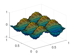
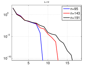
Figure 5.2. Rank decomposition of the solution for $12\times 12$ periodic coefficient.

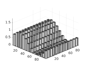
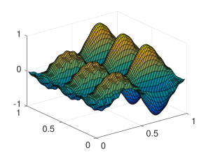
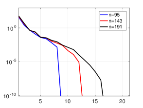
Figure 5.3. Rank decomposition of the solution for $12\times 12$ modulated periodic coefficient.

Further enhancement of the tensor approximation can be based on the application of the quantized-TT (QTT) tensor approximation which has been already applied in [23] to the 1D equations with quasi-periodic coefficients. The power of QTT approximation method is due to the perfect low rank decompositions applied to the wide class of function-related tensors [20], see [23] for the more detailed discussion and a number of numerical examples.

One can apply QTT approximations to problems with quasi periodic coefficients, which can be described by oscillation with smooth modulation around a constant value, oscillation around a given smooth function, or oscillation around piecewise constant function, see Figure 1.1 and examples in [23].

Let the vector ${\bf x}\in\mathbb{C}^{N}$, $N=2^{L}$, be obtained by sampling a continuous function $f\in C[0,1]$ (or even piecewise smooth functions), on the uniform grid of size $N$. For the following examples of univariate functions the explicit QTT-rank estimates of the corresponding QTT tensor representations are valid uniformly in the vector size $N$, see [20]:
(A) $r=1$ for complex exponentials, $f(x)=e^{i\omega x}$, $\omega\in\mathbb{R}$.
(B) $r=2$ for trigonometric functions, $f(x)=\sin{\omega x},f(x)=\cos{\omega x}$, $\omega\in\mathbb{R}$.
(C) $r\leq m+1$ for polynomials of degree $m$.
(D) For a function $f$ with the QTT-rank $r_{0}$ modulated by another function $g$ with the QTT-rank $r$ (say, step-type function, plain wave, polynomial) the QTT rank of a product $f\,g$ is bounded by a multiple of $r$ and $r_{0}$,

$$rank_{QTT}(fg)\leq rank_{QTT}(f)rank_{QTT}(g).$$

(E) Furthermore, the following result holds ([15]): QTT rank for the periodic amplification of a reference function on a unit cell to a rectangular lattice is of the same order as that for the reference function.

The rank of the QTT tensor representation to the 1D Galerkin FEM matrix in the case of oscillating coefficients was discussed in [14, 23].

5.3. Numerical test on the rank decomposition of ${\bf u}$

Figure 5.4 represents the right-hand side $f_{1}(x_{1},x_{2})$ and the respective solution for the discretization to equation (5.4) (with the coefficient depicted in Figure 5.1) on $400\times 400$-grid, where

$$f_{1}(x_{1},x_{2})=\sin(2x_{1})\sin(2x_{2}).$$

The PCG solver for the system of equations (5.8) with the discrete Laplacian inverse as the preconditioner demonstrates robust converges with the rate $q\ll 1$.

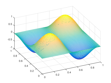
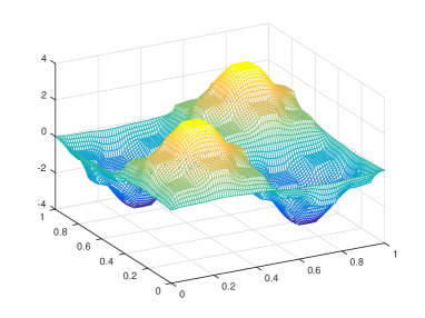
Figure 5.4. The right-hand side and solution for periodic oscillating coefficients shown in Figure 5.1.

Next example demonstrates the rank behavior in the singular value decomposition (SVD) of a matrix representing the solution vector ${\bf u}\in\mathbb{R}^{n_{1}\times n_{2}}$ to the equation (5.8) with $12\times 12$ periodic coefficient shown in Figure 5.2, left. Figure 5.5 represents the rank behavior in the SVD decomposition of the solution in the case of $8\times 8$ periodic coefficient.

It is worth to observe that comparison of Figures 5.2 and 5.5 indicates that the exponential decay of the approximation error in the rank parameter is stable with respect to the size of $L\times L$ lattice structure of the coefficient, i.e. the behavior of the singular values remains almost the same for different parameters $\epsilon=1/L$.

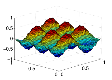
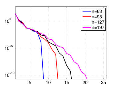
Figure 5.5. Accuracy of the rank decomposition of the solution vs. rank parameter for $8\times 8$ periodic coefficient and grid size $n\times n$.

Our iterative scheme includes only the matrix-vector multiplication with the stiffness matrix $A$ that has the small Kronecker rank $2R$, and the action of the preconditioner defined by the approximate inverse to the Laplacian type matrix. The latter has low Kronecker rank of order $R_{B}=O(|\log\varepsilon|^{2})$ as shown above.

Given rank-$1$ vector ${\bf u}={\bf u}_{1}\otimes{\bf u}_{2}$, the standard property of the Kronecker product matrices

$${A}{\bf u}={A}_{1}{\bf u}_{1}\otimes M_{2}{\bf u}_{2}+M_{1}{\bf u}_{1}\otimes{A}_{2}{\bf u}_{2},$$

indicates that the matrix-vector multiplication enlarges the initial rank by the factor of $2$ and similar with action of preconditioner. Hence each iterative step should be supplemented with certain rank truncation procedure which can be implemented adaptively to the chosen approximation threshold or fixed bound on the rank parameter.

Remark 5.1.

Notice that for $d=3$ the transformed matrix $A$ takes a form

$$A=A_{1}\otimes I_{2}\otimes I_{3}+I_{1}\otimes A_{2}\otimes I_{3}+I_{1}\otimes I_{2}\otimes A_{3},$$

and it obeys the $d$-term Kronecker sum representation in the general. Hence, in the general case of $d\geq 2$ and $R\geq 1$ the Kronecker rank of the matrix ${A}$ is given by

$$\mbox{rank}_{Kron}({A})=d\,R.$$

6. Conclusions

We present a preconditioned iteration method for solving an elliptic type boundary value problem in $\mathbb{R}^{d}$ with the operator generated by a quasi–periodic structure with rapidly changing coefficients characterized by a small length parameter $\epsilon$. We use tensor product FEM discretization that allows to approximate the stiffness matrix $A$ in the form of low-rank Kronecker sum. The preconditioner $\mathcal{A}_{0}$ is constructed based on certain averaging (homogenization) procedure of the initial equation coefficients such that inversion of $\mathcal{A}_{0}$ is much simpler than inversion of $\mathcal{A}$. We prove contraction of the iteration method and establish explicit estimates of the contraction factor $q<1$. For typical quasi–periodic structures we deduce fully computable two–sided a posteriori estimates which are able to control numerical solutions on any iteration.

We apply the tensor-structured approximation which is especially efficient if the equation coefficients admit low rank representations and algebraic operations are performed in tensor structured formats. Under moderate assumptions the storage and solution complexity of our approach depends only weakly (merely linear-logarithmically) on the frequency parameter $1/\epsilon$. Numerical tests demonstrate that the FEM solution allows the accurate low rank separable approximation which is the basic prerequisite for application of the tensor numerical methods to the problems of geometric homogenization.

The approach allows further enhancement based on the quantized-TT (QTT) tensor approximation which is the topic for future research work. Another direction is related to fully tensor structured implementation of the computable two–sided a posteriori error estimates.

Acknowledgements. SR appreciates the support provided by the Max-Planck Institute for Mathematics in the Sciences (Leipzig, Germany) during his scientific visit in 2016. The authors are thankful to Dr. V. Khoromskaia (MPI MIS, Leipzig) for the numerical experiments.

References

- [1] Bakhvalov, N. S., Panasenko, G. Homogenisation: Averaging Processes In Periodic Media: Mathematical Problems In The Mechanics Of Composite Materials. Springer, 1989.
- [2] P. Benner, V. Khoromskaia and B. N. Khoromskij. Range-separated tensor formats for numerical modeling of many-particle interaction potentials. E-preprint, http://arxiv.org/abs/1606.09218, 2016.
- [3] Bensoussan, A., Lions, J.-L., Papanicolaou, G. (1978): Asymptotic analysis for periodic structures. Amsterdam: North-Holland
- [4] S. Brenner and R. Scott. The mathematical theory of finite element methods. Springer, 1994.
- [5] J. P. Davis. Circulant matrices. New York. John Wiley & Sons, 1979.
- [6] Jikov, V.V., Kozlov, S.M., Oleinik, O.A. (1994): Homogenization of differential operators and integral functionals. Berlin: Springer
- [7] Friedman, A. (1976): Partial Differential Equations. R. E. Krieger Pub. Co., Huntington, NY
- [8] I.P. Gavrilyuk, W. Hackbusch and B.N. Khoromskij. Hierarchical Tensor-Product Approximation to the Inverse and Related Operators in High-Dimensional Elliptic Problems. Computing 74 (2005), 131-157.
-
[9]
Antoine Gloria and Felix Otto.
Quantitative estimates on the periodic approximation of the corrector in stochastic homogenization
In: ESAIM / Proceedings, 48 (2015), p. 80-97.
MIS-Preprint 12/2015, DOI: 10.1051/proc/201448003. - [10] R. Glowinski, J.-L. Lions, R. Trémolierés. Analyse numérique des inéquations variationnelles. Dunod, Paris, 1976.
- [11] Kantorovich L. V. and Krylov V. L., Approximate Methods of Higher Analysis. Interscience, New York, 1958.
- [12] V. Kazeev, I. Oseledets, M. Rakhuba, and Ch. Schwab. QTT-finite-element approximation for multiscale problems I: model problems in one dimension. Adv. Comput. Math., 2016. DOI: 10.1007/s10444-016-9491-y.
- [13] V. Kazeev, O. Reichmann, and Ch. Schwab. Low-rank tensor structure of linear diffusion operators in the TT and QTT formats. Linear Algebra and its Applications, v. 438(11), 2013, 4204-4221.
- [14] S. Dolgov, V. Kazeev, and B.N. Khoromskij. The tensor-structured solution of one-dimensional elliptic differential equations with high-dimensional parameters. Preprint 51/2012, MPI MiS, Leipzig 2012.
- [15] V. Khoromskaia and B. N. Khoromskij. Grid-based lattice summation of electrostatic potentials by assembled rank-structured tensor approximation. Comp. Phys. Commun., 185 (12), 2014, pp. 3162-3174.
- [16] V. Khoromskaia, and B.N. Khoromskij. Tensor Approach to Linearized Hartree-Fock Equation for Lattice-type and Periodic Systems. E-preprint arXiv:1408.3839, 2014.
- [17] V. Khoromskaia and B.N. Khoromskij. Fast tensor method for summation of long-range potentials on 3D lattices with defects. Numerical Linear Algebra with Applications, 2016, v. 23: 249-271.
- [18] V. Khoromskaia and B.N. Khoromskij. Tensor numerical methods in quantum chemistry: from Hartree-Fock to excitation energies. Phys. Chem. Chem. Phys., 17:31491 - 31509, 2015.
- [19] B.N. Khoromskij. Tensor-Structured Preconditioners and Approximate Inverse of Elliptic Operators in . J. Constr. Approx. 30 (2009) 599-620.
- [20] B.N. Khoromskij. -Quantics Approximation of - Tensors in High-Dimensional Numerical Modeling. Constr. Approx. 34 (2011) 257–280.
- [21] B.N. Khoromskij. Tensors-structured Numerical Methods in Scientific Computing: Survey on Recent Advances. Chemometr. Intell. Lab. Syst. 110 (2012), 1-19.
- [22] B.N. Khoromskij and G. Wittum. Numerical Solution of Elliptic Differential Equations by Reduction to the Interface. Research monograph, LNCSE, No. 36, Springer-Verlag, 2004.
- [23] B.N. Khoromskij and S. Repin. A fast iteration method for solving elliptic problems with quasiperiodic coefficients. Russ. J. Numer. Anal. Math. Modelling 2015; 30 (6):329-344. E-preprint arXiv:1510.00284, 2015.
- [24] B.N. Khoromskij, S. Sauter, and A. Veit. Fast Quadrature Techniques for Retarded Potentials Based on TT/QTT Tensor Approximation. Comp. Meth. in Applied Math., v.11 (2011), No. 3, 342 - 362.
- [25] J.-L. Lions and G. Stampacchia. Variational inequalities. Comm. Pure Appl. Math. 20 1967 493–519.
- [26] Ivan V Oseledets, and S.V. Dolgov. Solution of linear systems and matrix inversion in the TT-format. SIAM Journal on Scientific Computing, v. 34(5), 2012, A2718-A2739.
- [27] O. Mali, P. Neittaanmaki, S. Repin. Accuracy verification methods. Theory and algorithms. Springer, 2014
- [28] G. I. Marchuk and V. V. Shaidurov. Difference methods and their extrapolations. Applications of Mathematics, New York: Springer, 1983.
- [29] P. Neittaanmaki and S. Repin. Reliable methods for computer simulation. Error control and a posteriori estimates. Elsevier, 2004.
- [30] A. Ostrowski. Les estimations des erreurs a posteriori dans les procédés itératifs, C. R. Acad. Sci, Paris, Sér. A–B 275 (1972), pp. A275–A278.
- [31] S. Repin. A posteriori error estimation for variational problems with uniformly convex functionals, Math. Comput., 69(2000), 230, 481–500.
- [32] S. Repin. A Posteriori Estimates for Partial Differential Equations. Walter de Gruyter, Berlin, 2008.
- [33] S. Repin, T. Samrowski, and S. Sauter. A posteriori error majorants of the modeling errors for elliptic homogenization problems. C. R. Math. Acad. Sci. Paris 351 (2013), no. 23-24, 877-882
- [34] S. Repin, T. Samrowski, and S. Sauter. Combined a posteriori modeling-discretization error estimate for elliptic problems with complicated interfaces. ESAIM Math. Model. Numer. Anal., 46 (2012), no. 6, 1389-1405.
- [35] S. Repin, S. Sauter, and A. Smolianski. A posteriori estimation of dimension reduction errors for elliptic problems on thin domains. SIAM J. Numer. Anal. 42 (2004), no. 4, 1435–1451.
- [36] U. Schollwöck. The density-matrix renormalization group in the age of matrix product states, Ann.Phys. 326 (1) (2011) 96-192.
- [37] E. Zeidler. Nonlinear functional analysis and its applications. I. Fixed-point theorems, Springer-Verlag, New York, 1986.