Nonmodal stability analysis of the boundary layer under solitary waves

Abstract

In the present treatise, a stability analysis of the bottom boundary layer under solitary waves based on energy bounds and nonmodal theory is performed. The instability mechanism of this flow consists of a competition between streamwise streaks and two-dimensional perturbations. For lower Reynolds numbers and early times, streamwise streaks display larger amplification due to their quadratic dependence on the Reynolds number, whereas two-dimensional perturbations become dominant for larger Reynolds numbers and later times in the deceleration region of this flow, as the maximum amplification of two-dimensional perturbations grows exponentially with the Reynolds number. By means of the present findings, we can give some indications on the physical mechanism and on the interpretation of the results by direct numerical simulation in (Vittori & Blondeaux, 2008; Ozdemir et al., 2013) and by experiments in (Sumer et al., 2010). In addition, three critical Reynolds numbers can be defined for which the stability properties of the flow change. In particular, it is shown that this boundary layer changes from a monotonically stable to a non-monotonically stable flow at a Reynolds number of $\mbox{{Re}}_{\delta}=18$.

1 Introduction

In recent years, stability and transition processes in the boundary layer under solitary water waves have received increased attention in the coastal engineering community, cf. (Liu et al., 2007; Vittori & Blondeaux, 2008; Sumer et al., 2010; Ozdemir et al., 2013; Verschaeve & Pedersen, 2014). Motivated by the design of harbors and other coastal installations, this boundary layer is of importance for understanding sediment transport phenomena under water waves and scaling effects in experiments.

In the present treatise, the mechanisms leading to instability and finally to turbulent transition shall be investigated by means of a nonmodal stability analysis. The present boundary layer is not only of interest for the coastal engineering community, but can also serve as a useful generic flow for the investigation of stability and transition mechanisms of boundary layers displaying favorable and adverse pressure gradients, such as the ones developing in front and behind of the location of maximum thickness of an airplane wing or turbine blade profile. In addition, the present flow can be considered a model for the single stroke of a pulsating flow, such as Stokes’ second problem, which is of importance for biomedical applications.

Solitary waves, which are either found as surface or internal waves, are of great interest in the ocean engineering community for several reasons. They are nonlinear and dispersive. When frictional effects due to the boundary layer at the bottom and the top are negligible, the shape of solitary waves is preserved during propagation. Relatively simple approximate analytic solutions exist, see for instance Benjamin (1966), Grimshaw (1971) or Fenton (1972). In addition, these waves are relatively easy to reproduce experimentally. As such, they are often used in order to investigate the effect of a single crest of a train of waves.

The first works on the boundary layer under solitary waves aimed at estimating the dissipative effect on the overall wave (Shuto, 1976; Miles, 1980). The bottom boundary layer has been considered more relevant than the surface boundary layer for viscous dissipation (Liu & Orfila, 2004) and the stability of this boundary layer is also the subject of the present treatise.

The earliest experiments on the bottom boundary layer under solitary waves have been performed for internal waves by (Carr & Davies, 2006, 2010) and for surface waves by Liu et al. (2007). The latter showed that an inflection point develops in the deceleration region behind the crest of the wave. However, instabilities have not been observed in the experiments performed by them (Liu et al., 2007). In 2010, Sumer et al. used a water tunnel to perform experiments on the boundary layer under solitary waves. They observed three flow regimes. By means of a Reynolds number $\mbox{{Re}}_{\delta}$, defined by the Stokes length of the boundary layer and the characteristic particle velocity, as used in Ozdemir et al. (2013) and in the present treatise, these regimes can be characterized as follows. For small Reynolds numbers $\mbox{{Re}}_{\delta}<630$($\approx\mbox{{Re}}_{\rm Sumer}=2\cdot 10^{5}$, i.e. the Reynolds number defined in Sumer et al. (2010)), the flow does not display any instabilities and is close to the laminar solution given in Liu et al. (2007). For a Reynolds number in the range $630\leq\mbox{{Re}}_{\delta}<1000$ ($2\cdot 10^{5}\leq\mbox{{Re}}_{\rm Sumer}<5\cdot 10^{5}$), they observed the appearance of regularly spaced vortex rollers in the deceleration region of the flow. Increasing the Reynolds number further leads to a transitional flow displaying the emergence of turbulent spots growing together and causing transition to turbulence in the boundary layer. This happens at first in the deceleration region. However, the first instance of spot nucleation moves forward into the acceleration region of the flow for increasing Reynolds number. Sumer et al. did not control the level of external disturbances in their experiments nor did they report any information on its characteristics, such as length scale or intensity.

Almost parallel to the experiments by Sumer et al., Vittori and Blondeaux performed direct numerical simulations of this flow (Vittori & Blondeaux, 2008, 2011). Their results correspond roughly to the findings by Sumer et al. in that the flow in their simulations is first observed to display a laminar regime before displaying regularly spaced vortex rollers and finally becoming turbulent. However, the Reynolds numbers at which these regime shifts occur are larger than those in the experiments by Sumer et al.. In particular, Vittori and Blondeaux observed the flow to be laminar until a Reynolds number somewhat lower than $\mbox{{Re}}_{\delta}=1000$, after which the flow in their simulations displays regularly spaced vortex rollers. Transition to turbulence has been observed to occur for Reynolds numbers somewhat larger than $\mbox{{Re}}_{\delta}=1000$. They triggered the flow regime changes by introducing a random disturbance of a specific magnitude in the computational domain before the arrival of the wave. Ozdemir et al. (2013) performed direct numerical simulations using the same approach as Vittori and Blondeaux, but varied the magnitude of the initial disturbance. As a result they found different flow regimes than what Sumer et al. and Vittori and Blondeaux had observed. In the simulations by Özdemir et al. the flow stays laminar until $\mbox{{Re}}_{\delta}=400$, then enters a regime they called ’disturbed laminar’ for $400<\mbox{{Re}}_{\delta}<1500$, where instabilities can be observed. For $\mbox{{Re}}_{\delta}>1500$ regularly spaced vortex rollers appear in the deceleration region of the flow in their simulations giving rise to a $K$-type transition before turbulent break down, if the Reynolds number is large enough. A $K$-type transition is characterized by a spanwise instability giving rise to the development of $\Lambda$-vortices arranged in an aligned fashion, cf. Herbert (1988). For very large Reynolds numbers $\mbox{{Re}}_{\rm Sumer}>2400$, Özdemir et al. reported that the $K$-type transition is replaced by a transition which reminded them of a free stream layer type transition.

Next to investigations based on direct numerical simulations and experiments, modal stability theories have been employed in the works by Blondeaux et al. (2012), Verschaeve & Pedersen (2014) and Sadek et al. (2015). Employing a quasi-static approach for the Orr-Sommerfeld equation, cf. (von Kerczek & Davis, 1974), Blondeaux et al. found that this unsteady flow displayed unstable regions for all of their Reynolds number considered, even those deemed stable by direct numerical simulation.

In order to explain the divergences in transitional Reynolds numbers obtained by direct numerical simulation and experiment, Verschaeve & Pedersen (2014) performed a stability analysis in the frame of reference moving with the wave, where the present boundary layer flow is steady. For steady flows, well-established stability methods can be used. By means of the parabolized stability equation, they showed that for all Reynolds numbers considered in their analysis, the boundary layer displays regions of growth of disturbances. As the flow goes to zero towards infinity, there exists a point on the axis of the moving coordinate where the perturbations reach a maximum amplification before decaying again for a given Reynolds number. Depending on the level of initial disturbances in the flow, this maximum amount of amplification is sufficient for triggering secondary instability, such as turbulent spots or $\Lambda$-vortices, or not. This explains the diverging critical Reynolds numbers observed in direct numerical simulations and experiments for this boundary layer flow. A particular case in point, mentioned in Verschaeve & Pedersen (2014), is the experiment on the boundary layer under internal solitary waves by Carr & Davies (2006). Although, the amplitudes of the generated internal solitary waves in these experiments are relatively large compared to the thickness of the upper layer, the outer flow on the bottom is relatively well approximated by the first order solution of Benjamin (1966), cf. figure 12 in Carr & Davies (2006). In these experiments, the flow displays instabilities for Reynolds numbers much smaller than in the experiments by Sumer et al. (2010) or in the direct numerical simulations by Vittori & Blondeaux (2008) or Ozdemir et al. (2013). Verschaeve & Pedersen (2014) proposed, that due to the characteristic velocity of internal solitary waves being significantly smaller than that for surface solitary waves, they are expected to display instabilities much earlier for comparable levels of background noise.

Sadek et al. (2015) performed a similar modal stability analysis as Verschaeve & Pedersen (2014) by marching Orr-Sommerfeld eigenmodes forward in time using the linearized and two-dimensional nonlinear Navier-Stokes equations. They observed that only for Reynolds numbers larger than $\mbox{{Re}}_{\delta}=90$, Orr-Sommerfeld eigenmodes display growth and consequently defined this Reynolds number to be the critical Reynolds number where the flow changes from a stable to an unstable regime.

The modal stability theories employed in Blondeaux et al. (2012), Verschaeve & Pedersen (2014) and Sadek et al. (2015) capture only parts of the picture. In all of these works, only two-dimensional disturbances are considered. In addition, the amplifications computed in Verschaeve & Pedersen (2014) and Sadek et al. (2015) describe only the so-called exponential growth of the most unstable eigenfunction of the Orr-Sommerfeld equation. As shown in Butler & Farrell (1992); Trefethen et al. (1993); Schmid & Henningson (2001); Schmid (2007), perturbations can undergo significant transient growth even when modal stability theories predict the flow system to be stable. Nonmodal theory formulates the stability problem as an optimization problem for the perturbation energy. In the present treatise, optimal perturbations are computed for the unsteady boundary layer flow under a solitary wave, complementing the modal analysis performed in (Blondeaux et al., 2012; Verschaeve & Pedersen, 2014; Sadek et al., 2015). In particular, we shall investigate the following questions.

In Sadek et al. (2015), a critical Reynolds number is found based on a modal analysis. However, as perturbations can display growth even for cases where modal analysis predicts stability, this question needs to be treated in the framework of energy methods (Joseph, 1966). Using an energy bound derived in (Davis & von Kerczek, 1973), we shall show that a critical Reynolds number $\mbox{{Re}}_{A}>0$ can be found, such that for all Reynolds numbers smaller than $\mbox{{Re}}_{A}$, the flow is monotonically stable, meaning that all perturbations are damped for all times.

Ozdemir et al. (2013) supposed that a by-pass transition starts to develop in their simulations for some cases, but could not explain why then suddenly two-dimensional perturbations emerge producing a $K$-type transition typical for growing Tollmien-Schlichting waves. In the present treatise, we shall show that nonmodal theory is able to describe this competition between streaks and two-dimensional perturbations (i.e. nonmodal Tollmien-Schlichting waves), which allows us to predict the onset of growth of streaks and two-dimensional perturbations, their maximum amplification and the point in time when this maximum is reached. Furthermore, the dependence on the Reynolds number of the maximum amplification shall be investigated. The results obtained in the present treatise indicate why in the direct numerical simulations by Vittori & Blondeaux (2008, 2011) and Ozdemir et al. (2013), in all cases investigated, two dimensional perturbations lead to turbulent break-down, although one would expect, at least for some cases, turbulent break-down via three dimensional structures for a purely random seeding. On the other hand Sumer et al. (2010) observed the growth of two-dimensional structures only for a certain range of Reynolds numbers, before the appearance of turbulent spots. A $K$-type transition has not been observed in their experiments. Turbulent spots are in general attributed to the secondary instability of streamwise streaks, see for example (Andersson et al., 2001; Brandt et al., 2004). Though, the random break-down of Tollmien-Schlichting waves is also thought to produce turbulent spots, cf. (Shaikh & Gaster, 1994; Gaster, 2016). The present analysis is limited to the primary instability of streamwise streaks and nonmodal Tollmien-Schlichting waves. It gives, however, indications for a possible secondary instability mechanism of competing streaks and Tollmien-Schlichting waves.

The present treatise is organized as follows. In the following section, section 2, we describe the flow system and present equations for energy bounds and the nonmodal governing equations. The solutions of these equations applied to the present flow are presented and discussed in section 3. In section 4, we shall relate the current findings to results obtained previously in the literature. The present treatise is concluded in section 5.

2 Description of the problem

2.1 Specification of base flow

The outer flow of the present boundary layer is given by the celebrated first order solution for the inviscid horizontal velocity for solitary waves (Benjamin, 1966; Fenton, 1972). For a given point at the bottom, the outer flow can thus be written as in Sumer et al. (2010):

$$U_{\rm outer}^{*}(t^{*})=U_{0}{\rm sech}^{2}\left(\omega_{0}t^{*}\right).$$ (1)

In the limit of vanishing amplitude of the solitary wave, not only the nonlinearities in the inviscid solution become negligible, but they can also be neglected in the boundary layer equations. Following Liu & Orfila (2004), the horizontal component in the boundary layer $U_{\rm base}$ can be written as

$$U_{\rm base}=U_{\rm outer}+u_{bl},$$ (2)

where $u_{bl}$ contains the rotational part of the velocity and ensures that the no-slip boundary condition is satisfied. Neglecting the nonlinearities, we obtain the following boundary layer equations for $u_{bl}$ (Liu et al., 2007; Park et al., 2014):

$$\frac{\partial}{\partial t}u_{bl} = \frac{1}{2}\frac{\partial^{2}}{\partial z^{2}}u_{bl}$$ (3)

$$u_{bl}(0,t) = -U_{\rm outer}(t)$$ (4)

$$u_{bl}(\infty,t) = 0$$ (5)

$$u_{bl}(z,-\infty) = 0$$ (6)

Equation (3) is the linearized momentum equation. Equations (4) and (5) are the boundary conditions of the problem, with equation (4) representing the no-slip boundary condition and equation (5) representing the outer flow boundary condition. Equation (6) is the initial condition, which is advanced in time from $-\infty$. The resulting base flow $U_{\rm base}$, equation (2), is valid on the entire time axis $t\in(-\infty,\infty)$. The scaling used in equations (3-6) is given by $\omega_{0}$ for the time,

$$t=\omega_{0}t^{*},$$ (7)

by $U_{0}$ for the velocity,

$$U_{\rm outer}=\frac{1}{U_{0}}U_{\rm outer}^{*},$$ (8)

and by the Stokes boundary layer thickness $\delta$ for the wall normal variable $z$:

$$z=\frac{z^{*}}{\delta},$$ (9)

where

$$\delta=\sqrt{\frac{2\nu}{\omega_{0}}}.$$ (10)

For the solution of equations (3-6), a Shen-Chebyshev discretization in wall normal direction is chosen, whereas the resulting system is integrated in time by means of a Runge-Kutta integrator, cf. reference (Shen, 1995) and appendix A for details. Summing up, we consider solitary waves of small amplitudes for which formula (1) is a good approximation of the outer flow, such as the solitary wave experiments in Carr & Davies (2006, 2010); Liu et al. (2007) or the water channel experiments in Sumer et al. (2010) and Tanaka et al. (2011). As shown in Verschaeve & Pedersen (2014), for larger amplitude solitary waves the nonlinear effects are not negligible anymore and significant qualitative differences arise, making the present nonmodal approach not applicable anymore.

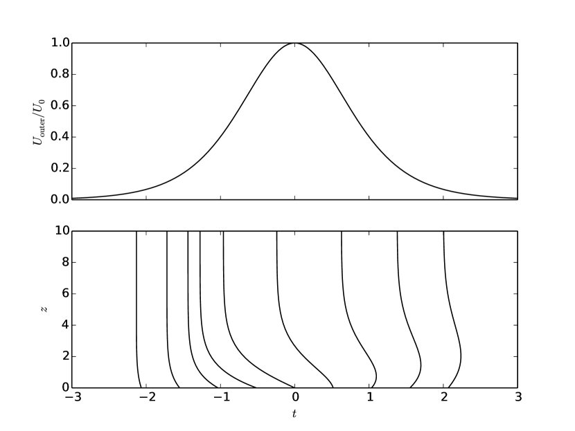
Figure 1: Inviscid outer flow $U_{\rm outer}$ at the bottom and profiles of the horizontal velocity component in the boundary layer under a solitary wave moving from right to left. The profiles have been multiplied by 40. The value at $z=0$ of the profiles shown corresponds to the point in time $t$, at which the profile has been taken. The horizontal velocity vanishes at $z=0$ in order to satisfy the no-slip boundary condition.

2.2 Stability analysis by means of an energy bound

In the present treatise, we use the same definition for the Reynolds number as in Ozdemir et al. (2013). This Reynolds number $\mbox{{Re}}_{\delta}$ is based on the Stokes length $\delta$ and the characteristic velocity $U_{0}$:

$$\mbox{{Re}}_{\delta}=\frac{U_{0}\delta}{\nu}=U_{0}\sqrt{\frac{2}{\nu\omega_{0}}},$$ (11)

where $\nu$ is the kinematic viscosity of the fluid. The Reynolds number $\mbox{{Re}}_{\rm Sumer}$ used in Sumer et al. (2010) is related to $\mbox{{Re}}_{\delta}$ by the following formula:

$$\mbox{{Re}}_{\delta}=\sqrt{2\mbox{{Re}}_{\rm Sumer}}.$$ (12)

We introduce a perturbation velocity $\mathbf{u}^{\prime}=(u^{\prime},v^{\prime},w^{\prime})$ in the streamwise, spanwise and wall normal direction, defined by:

$$\mathbf{u}^{\prime}=\left(u^{\prime},v^{\prime},w^{\prime}\right)=\left(u_{ns},v_{ns},w_{ns}\right)-\left(U_{\rm base}\left(z,t\right),0,0\right),$$ (13)

where $(u_{ns},v_{ns},w_{ns})$ satisfies the Navier-Stokes equations. The energy of the perturbation is given by:

$$E_{p}=\frac{1}{2}\int\limits_{V}u^{\prime 2}+v^{\prime 2}+w^{\prime 2}\,dV,$$ (14)

which is integrated over $V=\{(x,y,z)\,|\,z>0\}$. For time dependent flows in infinite domains, Davis & von Kerczek (1973) derived a bound for the perturbation energy of the nonlinear Navier-Stokes equations:

$$\frac{E_{p}(t)}{E_{p,0}}\leq\exp\frac{\mbox{{Re}}_{\delta}}{2}\int\limits_{t_{0}}^{t}\mu(t^{\prime})\,dt^{\prime},$$ (15)

where $\mu$ is the largest eigenvalue of the following linear system:

$$\frac{1}{\mbox{{Re}}_{\delta}}\Delta\mathbf{u}^{\prime}-\mathbf{S}_{\rm base}(t)\cdot\mathbf{u}^{\prime}-\nabla p = \frac{1}{2}\mu\mathbf{u}^{\prime}$$ (16)

$$\nabla\cdot\mathbf{u}^{\prime} = 0,$$ (17)

where the tensor $\mathbf{S}_{\rm base}$ is the rate of strain tensor given by the base flow, equation (2). We remark that Davis & von Kerczek (1973) appear to have overlooked a sign and a factor two in their equations. As the rate of strain tensor depends on time, the eigenvalue $\mu$ is a function of $t$. If $\mu<0$ for all times, then the flow is monotonically stable for this Reynolds number, meaning that all perturbations will decay for all times. This allows us to investigate, if there exists a Reynolds number $\mbox{{Re}}_{A}$, at which $\mu$ switches sign from negative to positive at some point in time. As the base flow is independent of $x$ and $y$, we consider a single Fourier component of $\mathbf{u}^{\prime}$:

$$(u^{\prime},v^{\prime},w^{\prime})(x,y,z,t)=(u,v,w)(z,t)\exp{\rm i}\left(\alpha x+\beta y\right).$$ (18)

This allows us to eliminate $p$ from the equations (16-17), resulting into

$$\frac{1}{\mbox{{Re}}_{\delta}}{\mathcal{L}}^{2}w+\frac{{\rm i}\alpha}{2}\left\{\frac{\partial^{2}}{\partial z^{2}}U_{\rm base}w+2\frac{\partial}{\partial z}U_{\rm base}\frac{\partial}{\partial z}w\right\}+\frac{{\rm i}\beta}{2}\frac{\partial}{\partial z}U_{\rm base}\zeta = \frac{1}{2}\mu{\mathcal{L}}w,$$ (19)

$$-\frac{1}{\mbox{{Re}}_{\delta}}{\mathcal{L}}\zeta-\frac{{\rm i}\beta}{2}\frac{\partial}{\partial z}U_{\rm base}w = \frac{1}{2}\mu(-\zeta)$$ (20)

where ${\mathcal{L}}$ is the Laplacian defined by:

$${\mathcal{L}}=-k^{2}+\frac{\partial^{2}}{\partial z^{2}},$$ (21)

where $k^{2}=\alpha^{2}+\beta^{2}$. The system of four equations (16-17), has been reduced to two, by means of the normal vorticity component $\zeta$:

$$\zeta={\rm i}\left(\alpha v-\beta u\right).$$ (22)

A Galerkin formulation for the system (19-20) is chosen based on Shen-Legendre polynomials for the biharmonic equation for the normal component $w$ and Shen-Legendre polynomials for the Poisson equation for the normal vorticity $\zeta$, cf. reference (Shen, 1994). Thereby, the Hermitian property of the system (19-20) is conserved in the discrete setting, guaranteeing purely real eigenvalues. Details of the implementation are given in appendix A.

2.3 The nonmodal stability equations

The nonmodal stability analysis is based on the linearized Navier-Stokes equations, which can be written in the present setting as follows,

$$\left(\frac{2}{\mbox{{Re}}_{\delta}}\frac{\partial}{\partial t}+{\rm i}\alpha U_{\rm base}-\frac{1}{\rm Re_{\delta}}\mathcal{L}\right)\mathcal{L}w-{\rm i}\alpha w\frac{\partial^{2}}{\partial z^{2}}U_{\rm base} = 0,$$ (23)

$$\left(\frac{2}{\mbox{{Re}}_{\delta}}\frac{\partial}{\partial t}+{\rm i}\alpha U_{\rm base}-\frac{1}{\rm Re_{\delta}}\mathcal{L}\right)\zeta-{\rm i}\beta w\frac{\partial}{\partial z}U_{\rm base} = 0.$$ (24)

We refer to Schmid & Henningson (2001); Schmid (2007) for a thorough derivation of equations (23) and (24). Given an initial perturbation $(w_{0},\zeta_{0})$ at time $t_{0}$, equations (23) and (24) can be integrated to obtain the temporal evolution of $(w,\zeta)$ for $t>t_{0}$. Nonmodal theory formulates the stability problem as finding the initial condition $(w_{0},\zeta_{0})$ maximizing the perturbation energy $E(t)$ of $(w,\zeta)$ at time $t>t_{0}$. This perturbation energy $E$ is the sum of two contributions, one from the wall normal component $w$ and one from the normal vorticity component $\zeta$:

$$E(t)=E_{w}(t)+E_{\zeta}(t)=\frac{1}{2}\int\limits_{0}^{\infty}\frac{1}{k^{2}}\left|\frac{\partial}{\partial z}w\right|^{2}+\left|w\right|^{2}\,dz+\frac{1}{2}\int\limits_{0}^{\infty}\frac{1}{k^{2}}\left|\zeta\right|^{2}\,dz.$$ (25)

The optimization problem can then be formulated by maximizing $E$ for a perturbation $(w,\zeta)$ satisfying (23) and (24) and having an initial energy $E_{0}$. One way of solving this optimization problem is by means of the adjoint equation as in Luchini & Bottaro (2014). Another approach for finding the optimal perturbation, which is employed in the present treatise, consists in formulating the discrete problem first and computing the evolution matrix $\mathbf{X}(t,t_{0})$ of the system of ODEs, cf. references Trefethen et al. (1993); Schmid & Henningson (2001); Schmid (2007) for details. The energy $E$ is then given in terms of $\mathbf{X}$ and the initial condition. Details of the implementation are given in appendix A. By computing $E(t)$ one way or the other, we can compute the amplification $G$ from time $t_{0}$ to $t$ of the optimal perturbation for wave numbers $\alpha$ and $\beta$:

$$G(\alpha,\beta,t_{0},t,\mbox{{Re}}_{\delta})=\max_{(w_{0},\zeta_{0})}\frac{E(t)}{E(t_{0})}.$$ (26)

We remark that the initial condition $(w_{0},\zeta_{0})$ from which the optimal perturbation starts, might be different for each point in time $t$, when tracing $G$ as a function of $t$, cf. section 3. The maximum amplification $G_{\max}(\mbox{{Re}}_{\delta})$, which can be reached for a given Reynolds number $\mbox{{Re}}_{\delta}$, is obtained by maximizing $G$ over time, initial time and wavenumbers:

$$G_{\max}=\max_{\alpha,\beta,t_{0},t}G.$$ (27)

In the following, we shall distinguish between three types of perturbations:

• streamwise streaks.
  These are perturbations independent of the streamwise coordinate $x$. They can be computed by setting $\alpha=0$.

• Two-dimensional perturbations.
  These perturbations are independent of the spanwise coordinate $y$ and can be computed by setting $\beta=0$. In this case, equations (23) and (24) are decoupled. These two-dimensional perturbations can be considered nonmodal Tollmien-Schlichting waves resulting from an optimization of the initial conditions of (23) and (24). Therefore, they display larger growth than modal Tollmien-Schlichting waves resulting from the Orr-Sommerfeld equation. This shall be presented more in detail in section 4.

• Oblique perturbations.
  These are all remaining perturbations with $\alpha\neq 0$ and $\beta\neq 0$.

3 Results and discussion

3.1 Monotonic stability

In this section, we shall determine the critical Reynolds number $\mbox{{Re}}_{A}$ behind which perturbations display growth. To this aim, the energy criterion in Davis & von Kerczek (1973) shall be used. We solve equations (19) and (20) for a given pair of wave numbers $(\alpha,\beta)$ and note the Reynolds number $\mbox{{Re}}_{\delta}$ for which the largest eigenvalue $\mu$ changes from minus to plus. At first, we compute the curves of critical Reynolds numbers $\mbox{{Re}}_{\delta}(\alpha)$ and $\mbox{{Re}}_{\delta}(\beta)$ by setting $\beta=0$ and $\alpha=0$, respectively. These curves are plotted in figure 2. As it turns out, all other cases, i.e. $\alpha\neq 0$ and $\beta\neq 0$, have their critical Reynolds number lying in the region between these two curves. From figure 2, we can infer that the flow is monotonically stable for all Reynolds numbers $\mbox{{Re}}_{\delta}$ smaller than $\mbox{{Re}}_{A}=18$. The physical significance of this critical Reynolds number is, however, limited. For example, the water depth of a surface solitary wave with amplitude ratio $\epsilon=0.1$ would be approximately $1\,{\rm cm}$ for this case. For these small water depths, other physical effects, such as capillary effects and not least the dissipative effect of the boundary layers on the solitary wave, are not negligible anymore. The solitary wave solution would thus not be valid in the first place. From figure 2, we observe that streamwise streaks will grow first. Two-dimensional perturbations, on the other hand, can only grow for flows with a Reynolds number larger than $\mbox{{Re}}_{B}=38$.

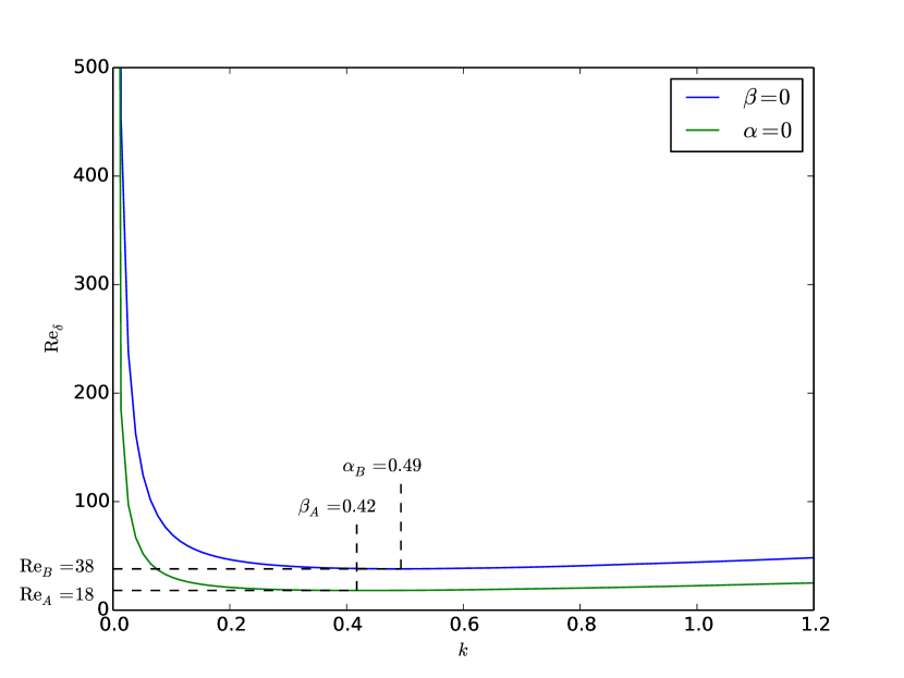
Figure 2: Isolines of $\mu=0$ for the energy bound of Davis & von Kerczek (1973), equations (19) and (20), as a function of the wave number $k^{2}=\alpha^{2}+\beta^{2}$ and the Reynolds number $\mbox{{Re}}_{\delta}$. The blue and green lines correspond to the cases $\beta=0$ and $\alpha=0$, respectively. All other cases have their critical Reynolds number in the space between these lines.

3.2 Optimal perturbation

3.2.1 Theoretical considerations

Before turning to the computation of the amplification $G$, equation (26), we shall first consider a scaling argument, as in Gustavsson (1991); Schmid & Henningson (2001). For streamwise streaks ($\alpha=0$), equations (23) and (24) can be written as:

$$\left(\frac{\partial}{\partial t}-\frac{1}{2}\mathcal{L}\right)\mathcal{L}{w} = 0,$$ (28)

$$\left(\frac{\partial}{\partial t}-\frac{1}{2}\mathcal{L}\right)\tilde{\zeta}-{\rm i}\beta{w}\frac{\partial}{\partial z}U_{\rm base} = 0,$$ (29)

where $\tilde{\zeta}$ is scaled by $\mbox{{Re}}_{\delta}/2$:

$$\tilde{\zeta}=\frac{2}{\mbox{{Re}}_{\delta}}\zeta(z,t).$$ (30)

Equation (28) corresponds to slow viscous damping of $w$, as also the homogeneous part of equation (29) for $\tilde{\zeta}$. On the other hand the second term in (29) represents a forcing term which varies on the temporal scale of the outer flow. Therefore, streamwise streaks display temporal variations on the time scale of the outer flow. As for steady flows (Gustavsson, 1991; Schmid & Henningson, 2001), the energy $E_{\zeta}$ is proportional to the square of the Reynolds number for the present unsteady flow:

$$E_{\zeta}\propto\mbox{{Re}}_{\delta}^{2}.$$ (31)

For large Reynolds numbers $E_{\zeta}$ will dominate. Therefore, the maximum amplification $G$ for streamwise streaks is expected to behave as

$$\max_{\beta,t_{0},t}G(\alpha=0,\beta,t_{0},t,\mbox{{Re}}_{\delta})\approx\mbox{{Re}}^{2}_{\delta}\quad\mbox{{Re}}_{\delta}>>1.$$ (32)

This quadratic growth of streamwise streaks can be contrasted to the exponential growth of $E_{w}$ for perturbations with $\alpha>0$, as we shall see in the following. To this aim, we use a decomposition (or integrating factor) as in the parabolized stabiltiy equation (Bertolotti et al., 1992) for the normal velocity component $w$:

$$w=\tilde{w}(z,t)\exp\int\limits_{t_{0}}^{t}\omega(t^{\prime})\,dt^{\prime},$$ (33)

where the imaginary part of $\omega$ accounts for the oscillatory character of $w$ and the real part of $\omega$ is the growth rate of the perturbation. In order to define the shape function $\tilde{w}$ univocally, all growth is restricted to $\omega$. Somewhat different to (Bertolotti et al., 1992), we define the normalization condition on the entire kinetic energy $\tilde{E}$ of the shape function $\tilde{w}$ :

$$\tilde{E}=\frac{1}{2}\int\limits_{0}^{\infty}\frac{1}{k^{2}}|D\tilde{w}|^{2}+|\tilde{w}|^{2}\,dz,$$ (34)

where we have write $D=\partial/\partial z$. Thus, the normalization constraint on $\tilde{w}$ is given by the following two conditions:

$$\int\limits_{0}^{\infty}\frac{\partial\tilde{w}^{\dagger}}{\partial t}\mathcal{L}\tilde{w}\,dz=\int\limits_{0}^{\infty}\tilde{w}^{\dagger}\mathcal{L}\frac{\partial\tilde{w}}{\partial t}\,dz=0$$ (35)

From this, it follows, that we can define the energy of the shape function to be unity for all times:

$$\frac{\partial}{\partial t}\int\limits_{0}^{\infty}\tilde{w}^{\dagger}\mathcal{L}\tilde{w}\,dz=0\quad\mbox{or}\quad\tilde{E}=-\frac{1}{2k^{2}}\int\limits_{0}^{\infty}\tilde{w}^{\dagger}\mathcal{L}\tilde{w}\,dz=1.$$ (36)

Equation (23) becomes then:

$$\partial_{t}\mathcal{L}\tilde{w}+\omega\mathcal{L}\tilde{w}=\frac{1}{2}\mathcal{L}^{2}\tilde{w}+{\rm i}\alpha\frac{1}{2}\mbox{{Re}}_{\delta}\left(D^{2}U_{0}-U_{0}\mathcal{L}\right)\tilde{w}$$ (37)

Multiplying by $\tilde{w}^{\dagger}$ and integrating in $z$, leads to a formula for $\omega$:

$$\omega=-\frac{1}{4k^{2}}\int\limits_{0}^{\infty}\tilde{w}^{\dagger}\mathcal{L}^{2}\tilde{w}\,dz-\frac{{\rm i}\alpha}{4k^{2}}\mbox{{Re}}_{\delta}\int\limits_{0}^{\infty}\tilde{w}^{\dagger}D^{2}U_{\rm base}\tilde{w}-\tilde{w}^{\dagger}U_{\rm base}\mathcal{L}\tilde{w}\,dz$$ (38)

The growth rate, ie. the real part of $\omega$, is given by:

$$\omega_{r}=-\frac{1}{4k^{2}}\int\limits_{0}^{\infty}\mathcal{L}\tilde{w}^{\dagger}\mathcal{L}\tilde{w}\,dz+\mbox{{Re}}_{\delta}\frac{\alpha}{4k^{2}}\int\limits_{0}^{\infty}DU_{\rm base}\left\{\tilde{w}_{r}D\tilde{w}_{i}-\tilde{w}_{i}D\tilde{w}_{r}\right\}\,dz$$ (39)

The first term on the right hand side represents viscous dissipation and is always negative. The second term, however, can, depending on $U_{\rm base}$ and $\tilde{w}$, be positive or negative. Only when this term is positive and in magnitude larger than the viscous dissipation, growth of $E_{w}$ can be observed. We observe that this term is multiplied by $\alpha/(\alpha^{2}+\beta^{2})$, which for a given $\alpha$ is maximal for $\beta=0$. This indicates that the possible growth rate for two-dimensional perturbations is larger than that for oblique perturbations when considering exponential growth in $E_{w}$ and neglecting quadratic growth in $E_{\zeta}$. We shall return to this point, when discussing the numerical results. For the decomposition in equation (33), the continuity equation can be written as:

$${\rm i}\alpha\tilde{u}+{\rm i}\beta\tilde{v}=-D\tilde{w},$$ (40)

where we have normalized the horizontal velocities:

$$\tilde{u}=u\exp-\int\limits_{t_{0}}^{t}\omega\,dt^{\prime},\quad\tilde{v}=v\exp-\int\limits_{t_{0}}^{t}\omega\,dt^{\prime}.$$ (41)

Then the growth rate $\omega_{r}$, equation (39), can be written as:

$$\omega_{r} = -\frac{1}{4k^{2}}\int\limits_{0}^{\infty}|\mathcal{L}\tilde{w}|^{2}\,dz-\frac{\mbox{{Re}}_{\delta}}{4}\int\limits_{0}^{\infty}\left(\tilde{u}^{\dagger}_{k},\tilde{w}^{\dagger}\right)\mathbf{S}_{k}\left(\begin{array}[]{c}\tilde{u}_{k}\\ \tilde{w}\end{array}\right),$$ (44)

where $\tilde{u}_{k}$ is the projection of the horizontal velocity vector onto the wavenumber vector $\mathbf{k}=(\alpha,\beta)$,

$$\tilde{u}_{k}=\frac{1}{k}\left(\alpha\tilde{u}+\beta\tilde{v}\right),$$ (45)

and $\mathbf{S}_{k}$, the two dimensional rate of strain tensor of the projection of the base flow on the wavenumber vector $\mathbf{k}$:

$$\mathbf{S}_{k}=\frac{1}{2}\left(\begin{array}[]{cc}0&DU_{k}\\ DU_{k}&0\end{array}\right),\quad U_{k}=\frac{1}{k}\alpha U_{\rm base}.$$ (46)

When considering two-dimensional perturbations ($\beta=0$), the growth rate $\omega_{r}$ simplifies to

$$\omega_{r} = -\frac{1}{4\alpha^{2}}\int\limits_{0}^{\infty}|\mathcal{L}\tilde{w}|^{2}\,dz-\frac{\mbox{{Re}}_{\delta}}{4}\int\limits_{0}^{\infty}\left(\tilde{u}^{\dagger},\tilde{w}^{\dagger}\right)\mathbf{S}_{2D}\left(\begin{array}[]{c}\tilde{u}\\ \tilde{w}\end{array}\right),$$ (49)

where the $\mathbf{S}_{2D}$ is the two-dimensional rate of strain tensor of the base flow:

$$\mathbf{S}_{2D}=\frac{1}{2}\left(\begin{array}[]{cc}0&DU_{\rm base}\\ DU_{\rm base}&0\end{array}\right).$$ (50)

In this case (ie. $\beta=0$), equations (23) and (24) are decoupled. As can be seen from equation (24), the normal vorticity $\zeta$ experiences only dampening. Growth can, therefore, only arise in the energy $E_{w}$ associated to the normal velocity component $w$, equation (25). As mentioned above, the first term on the right hand side in equation (49) is always negative and represents the viscous dissipation stabilizing the flow. As the eigenvalues of $\mathbf{S}_{2D}$ are given by $DU_{\rm base}/2$ and $-DU_{\rm base}/2$, the second term on the right hand side in equation (49) can, depending on $\tilde{w}$, be positive or negative. All possible growth of two-dimensional perturbations is thus due to the second term where the velocity vector $\left(\tilde{u},\tilde{w}\right)^{T}$ is being tilted by the rate of strain tensor $\mathbf{S}_{2D}$. Equation (49) is an illustrative formula for the Orr-mechanism. The growth mechanism itself is thus always inviscid. This holds for any two-dimensional perturbation, also those being the eigenfunctions of the Orr-Sommerfeld equation, the modal Tollmien-Schlichting waves, which are commonly thought of as slow viscous instabilities, cf. for example (Jimenez, 2013) and (Brandt et al., 2004). Whether growth of two-dimensional perturbations is fast or slow is, as formula (49) suggests, primarily a property of the base flow profile $U_{\rm base}$. As we shall see below, velocity profiles having an inflection point allow for larger growth rates than profiles without.

As the Reynolds number multiplies the second term in equation (49), we can conclude that for large $\mbox{{Re}}_{\delta}$, the maximum amplification of two-dimensional perturbations roughly behaves like:

$$\max_{\alpha,t_{0},t}G(\alpha,\beta=0,t_{0},t,\mbox{{Re}}_{\delta})\approx e^{c\mbox{{Re}}_{\delta}},\quad\mbox{{Re}}_{\delta}>>1$$ (51)

where $c$ is some constant. This exponential growth of the maximum amplification with the Reynolds number has also been observed for other flows displaying an adverse pressure gradient. For example, Biau (2016) observed that the maximum amplification of two-dimensional perturbations for Stokes’ second problem grows exponentially with the Reynolds number.

In the following, we shall see that the competition of the maximum amplification between the quadratic growth in $\mbox{{Re}}_{\delta}$ of streamwise streaks, equation (32), and the exponential growth in $\mbox{{Re}}_{\delta}$ of two-dimensional structures, equation (51), composes the essential primary instability mechanism of this flow.

3.2.2 Numerical results

The amplification $G$, equation (26), for the present flow problem depends on five parameters, the wavenumbers $\alpha$ and $\beta$, the initial time $t_{0}$, the time $t$ and the Reynolds number $\mbox{{Re}}_{\delta}$. We start our numerical analysis by tracing the evolution of $\max_{\alpha,\beta}G$ for a given Reynolds number $\mbox{{Re}}_{\delta}$ and a given initial time $t_{0}$. In figure 3, we plot the temporal evolution of $\max_{\alpha,\beta}G$ for the Reynolds numbers $\mbox{{Re}}_{\delta}=141,316,447$ and $1000$ ($\mbox{{Re}}_{\rm Sumer}=10^{4},5\cdot 10^{4},10^{5},5\cdot 10^{5}$) and initial times $t_{0}=-8,-6,\ldots,6$. For the case $\mbox{{Re}}_{\delta}=141$, cf. figure 3a, we observe that growth of perturbations is mainly restricted to the deceleration region of the flow, i.e. where $t>0$. Only the optimal perturbation starting at $t_{0}=-2$ displays some growth before the arrival of the crest of the solitary wave. Among the initial conditions $t_{0}$ chosen, the optimal perturbation with $t_{0}=0$ displays the maximum amplification at $t_{\max}=1.5$ with $G\approx 20$. This is due to the acceleration region of the flow ($t<0$) having a damping effect on the perturbations starting before $t=0$. On the other hand the perturbations starting at later times $t_{0}\geq 2$ already miss out a great deal of the destabilizing effect of the adverse pressure gradient. All curves display a maximum at some time. For some cases, this maximum lies outside of the plotting domain. For a slightly larger Reynolds number, cf. figure 3b with $\mbox{{Re}}_{\delta}=316$, we observe a qualitatively similar behavior for the perturbations starting at $t_{0}<0$ with the difference that growth of these perturbations sets in somewhat earlier in time than in the $\mbox{{Re}}_{\delta}=141$ case and leads also to higher amplifications. However, the optimal perturbation starting at $t_{0}=0$ behaves differently than the corresponding one for the $\mbox{{Re}}_{\delta}=141$ case. At early times, i.e. for $t\lesssim 2$, the evolution of this perturbation is similar to the $\mbox{{Re}}_{\delta}=141$ case. The perturbation grows to a maximum $G\approx 100$ at $t\approx 1.5$, before decaying again, but, at time $t\approx 2$, the amplification curve displays a kink and a sudden growth to $G\approx 2000$ at time $t_{\max}=8.2$. A similar, however, less expressive kink is also visible in the curve for $t_{0}=2$. Increasing the Reynolds number to $\mbox{{Re}}_{\delta}=447$, cf. figure 3c, does not change the picture qualitatively. However, the maximum amplification of the optimal perturbation starting at $t_{0}=0$ has increased by a factor of approximately thousand compared to the $\mbox{{Re}}_{\delta}=316$ case. In comparison, the maximum of the optimal perturbation starting at $t_{0}=-2$ has only increase by a factor of approximately 1.25 when going from $\mbox{{Re}}_{\delta}=316$ to $\mbox{{Re}}_{\delta}=447$. This violent growth for the optimal perturbation starting at $t_{0}$ is also visible for the $\mbox{{Re}}_{\delta}=1000$ case, cf. figure 3d. However, for this case, even the curves of the perturbations starting at earlier times display a similar kink and sudden growth in the deceleration region.

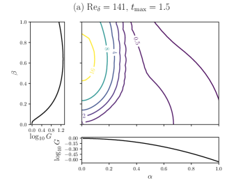
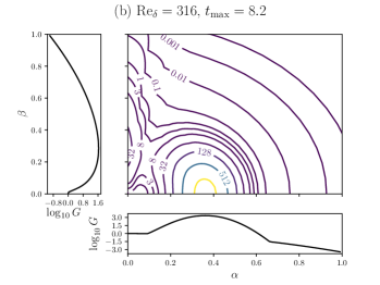
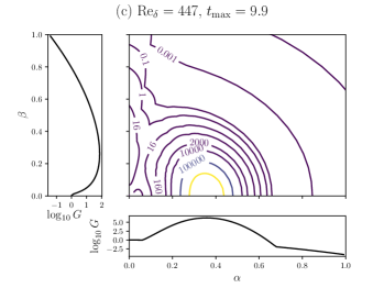
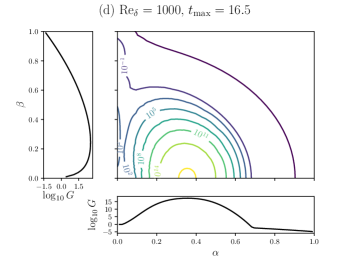
Figure 4: Contour plots of the amplification $G(\alpha,\beta,t_{0}=0,t_{\max},\mbox{{Re}}_{\delta})$ at $t_{\max}=1.5,8.2,9.9,16.5$ for the cases $\mbox{{Re}}_{\delta}=141,316,447,1000$, respectively. The plots to the left and below the contour plot show a slice along the $\beta$- and $\alpha$-axes, respectively.

In figure 4, we show contour plots of the amplification $G(\alpha,\beta,t_{0}=0,t_{\max},\mbox{{Re}}_{\delta})$ at $t_{\max}=1.5,8.2,9.9,16.5$ for the cases $\mbox{{Re}}_{\delta}=141,316,447,1000$, respectively. For the case $\mbox{{Re}}_{\delta}=141$, cf. figure 4a, we find a single maximum lying on the $\beta$-axis. On the other hand, the $\mbox{{Re}}_{\delta}=316$ case is different, cf. figure 4b. Whereas all two-dimensional perturbations display decay at $t_{\max}=1.5$ for the $\mbox{{Re}}_{\delta}=141$ case, the amplification of two-dimensional perturbations displays a peak at around $\alpha=0.35$ for the $\mbox{{Re}}_{\delta}=316$ case. A second peak, lying on the $\beta$ axis, is significantly smaller than the peak of two-dimensional perturbations on the $\alpha$-axis. Increasing the Reynolds number, cf. figures 4c and 4d, increases the magnitude of the peaks, with the peak on the $\alpha$-axis growing faster with $\mbox{{Re}}_{\delta}$ than the peak on the $\beta$-axis. This competition between streamwise streaks and two-dimensional structures is characteristic for flows with adverse pressure gradients and has also been observed for steady flows. The Falkner-Skan boundary layer with adverse pressure gradient displays contour levels similar to the present ones, cf. for example Levin & Henningson (2003, figure 10d) or Corbett & Bottaro (2000). Another example is the flow of three dimensional swept boundary layers investigated in Corbett & Bottaro (2001).

The competition between streamwise streaks and two-dimensional perturbations can also be observed in the temporal evolution of the amplification of the optimal perturbation. In figure 5, we compare the temporal evolution of $\max_{\beta}G(\alpha=0,\beta,t_{0}=0,t,\mbox{{Re}}_{\delta}=316)$, $\max_{\alpha}G(\alpha,\beta=0,t_{0}=0,t,\mbox{{Re}}_{\delta}=316)$ and $\max_{\alpha,\beta}G(\alpha,\beta,t_{0}=0,t,\mbox{{Re}}_{\delta}=316)$. For early times ($0<t\lesssim 2$) the streamwise streaks display a larger amplification than the two-dimensional perturbations, but at time $t\approx 2$, the two-dimensional perturbations overtake the streaks. Maximizing over $\alpha$ and $\beta$, chooses either perturbation displaying maximum amplification. The amplification of oblique perturbations seems to be most often smaller than that of streamwise streaks or two-dimensional perturbations. This allows us to trace the maximum amplification $G_{\max}$, equation (27), by considering only the amplification of the cases $(\alpha=0,\beta)$ and $(\alpha,\beta=0)$ instead of maximizing over all possible wave numbers $(\alpha,\beta)$. Growth of streamwise streaks is associated to the lift-up effect (Ellingsen & Palm, 1975), whereas the growth of two-dimensional perturbations is associated to the Orr-mechanism (Jimenez, 2013). We remark that other growth mechanisms exists, such as the Reynolds stress mechanism, cf. Butler & Farrell (1992), which can lead to the maximum amplification of streaks not being exactly on the $\beta$ axis, but having a non-zero $\alpha$-component. However, as also shown for other flows (Butler & Farrell, 1992), this $\alpha$-component is negligibly small and, therefore, not considered in the present treatise. In figure 6, the amplification of streamwise streaks and two-dimensional perturbations maximized over the initial time $t_{0}$ and time $t$ is plotted against the Reynolds number. As predicted in section 3.1 by the energy bound of Davis & von Kerczek (1973), streamwise streaks start to grow for Reynolds numbers larger than $\mbox{{Re}}_{A}=18$, whereas two-dimensional perturbations start growing for $\mbox{{Re}}_{B}>38$. We can define a third critical Reynolds number $\mbox{{Re}}_{C}=170$ for this flow, which stands for the value when the maximum amplification of two-dimensional perturbations overtakes the maximum amplification of streamwise streaks. This happens for rather low levels of amplification, the maximum amplification being $G_{\max}=28$ for $\mbox{{Re}}_{\delta}=170$. As in Biau (2016) for Stokes second problem, the amplification of two-dimensional perturbations is observed to be exponential. For flows with a Reynolds number larger than $\mbox{{Re}}_{C}$, which are most relevant cases, the dominant perturbations are therefore likely to be two-dimensional (up to secondary instability). This supports the observation by Vittori & Blondeaux (2008) and Ozdemir et al. (2013) of a transition process via the development of two-dimensional vortex rollers. However, when starting early, i.e. for initial times $t_{0}<-1$, streamwise streaks start growing before two-dimensional structures, as can be seen in figure 3d. The competition between streamwise streaks and two-dimensional structures to first reach secondary instability, might therefore not only be determined by the maximum amplification reached, but also by the point in time, when the amplification of the perturbation is sufficient to trigger secondary instability, be it streaks or two-dimensional perturbations. We shall discuss this point further in section 4.

When plotting the maximum amplification of streamwise streaks in a log-log plot, cf. figure 7, we find the expected quadratic behavior of the maximum amplification. In line with this quadratic growth in $\mbox{{Re}}_{\delta}$, a straightforward calculation, cf. appendix B, shows that when normalizing the energy $E=E_{w}+E_{\zeta}$, equation (25) of the initial condition of the optimal streamwise streak to one, the amplitude of the initial normal vorticity scales inversely with the Reynolds number, whereas the amplitude of the normal velocity converges to a constant in the asymptotic limit:

$$\max_{z}\zeta(z,t_{0})\propto\frac{1}{\mbox{{Re}}_{\delta}},\quad\max_{z}w(z,t_{0})\propto{\rm const}\quad\mbox{for}\quad\mbox{{Re}}_{\delta}\rightarrow\infty.$$ (52)

This can also be observed in figure 8, where we show that for larger Reynolds numbers, the graphs of $|\zeta|\cdot\mbox{{Re}}_{\delta}$ and $|w|$ collapse. In order to visualize the spatial structure of the optimal streamwise streak, we consider the case $\mbox{{Re}}_{\delta}=500$ with a maximum amplification of:

$$\max_{\beta,t_{0},t}G(\alpha=0,\beta,t_{0},t,\mbox{{Re}}_{\delta}=500)=238.6,$$ (53)

where the parameters at maximum are given by:

$$\beta=0.64,\quad t_{0}=0.11,\quad t=1.53.$$ (54)

In figure 9, contour plots of the real part of the initial condition at $t_{0}=0.11$ of the optimal perturbation in the $(y,z)$-plane is shown. When advancing this initial condition to $t=1.53$, where the energy of the streamwise streak is maximum, cf. figure 10, we observe that the amplitude of the normal velocity component $w$ has decreased by approximately a factor of two, whereas the amplitude of the normal vorticity $\zeta$ increased by approximately a factor of five hundred.

For two-dimensional perturbations, on the other hand, the energy is distributed between the normal component $w$ and the horizontal component $u={\rm i}Dw/\alpha$. As can be observed from figure 11, for increasing Reynolds number the amplitude of $w$ decreases. Following, its share of the initial energy goes down as well. Since the initial energy is normalized to one, this implies that the energy contribution associated to $u$ must increase. Corresponding to this energy increase, we observe that the amplitude of $u$ increases for increasing Reynolds number, cf. figure 12. We choose the case $\mbox{{Re}}_{\delta}=1000$ in order to visualize the spatial structure of the optimal two-dimensional perturbation. For this case the maximum amplification is given by:

$$\max_{\alpha,t_{0},t}G(\alpha,\beta=0,t_{0},t,\mbox{{Re}}_{\delta}=1000)=1.34\cdot 10^{18},$$ (55)

where the parameters at maximum are given by:

$$\alpha=0.33,\quad t_{0}=0.26,\quad t=14.2.$$ (56)

In figure 13, contour plots in the $(x,z)$-plane of the real part of $w\cdot\exp{\rm i}\alpha x$ at initial time $t_{0}$ and at time $t$ when it reaches maximal amplification are plotted. Initially, the perturbation is confined to a thin layer inside the boundary layer. While reaching its maximum amplification its spatial structure grows in wall normal direction.

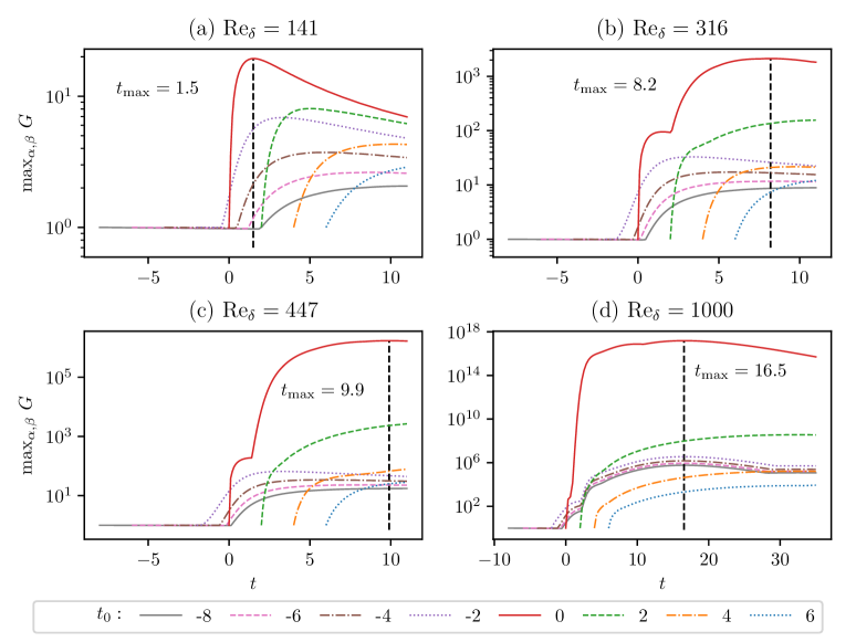
Figure 3: Temporal evolution of the amplification $G$ maximized over the wavenumbers $\alpha$ and $\beta$ for different Reynolds numbers $\mbox{{Re}}_{\delta}$ and initial times $t_{0}$.

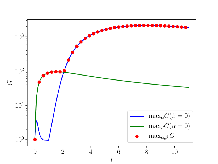
Figure 5: Temporal evolution of $\max_{\beta}G(\alpha=0,\beta,t_{0}=0,t,\mbox{{Re}}_{\delta}=316)$, $\max_{\alpha}G(\alpha,\beta=0,t_{0}=0,t,\mbox{{Re}}_{\delta}=316)$ and $\max_{\alpha,\beta}G(\alpha,\beta,t_{0}=0,t,\mbox{{Re}}_{\delta}=316)$.

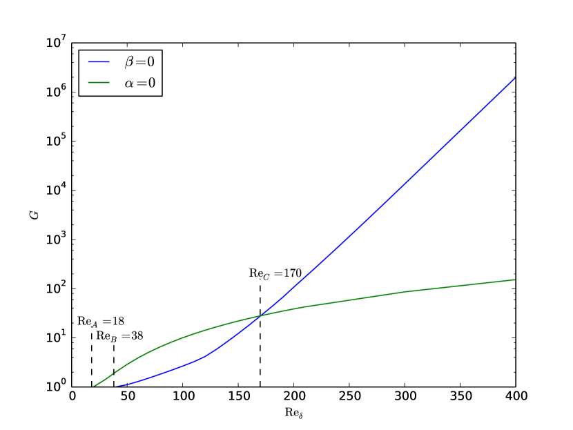
Figure 6: Maximum amplification of streamwise streaks $\max_{\beta,t_{0},t}G(\alpha=0,\beta,t_{0},t,\mbox{{Re}}_{\delta})$ and two-dimensional perturbations $\max_{\alpha,t_{0},t}G(\alpha,\beta=0,t_{0},t,\mbox{{Re}}_{\delta})$.

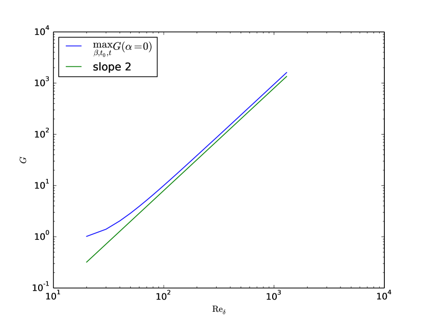
Figure 7: Maximum amplification of streamwise streaks, $\max_{\beta,t_{0},t}G(\alpha=0,\beta,t_{0},t,\mbox{{Re}}_{\delta})$, versus Reynolds number.

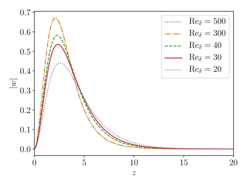
(a) $w$

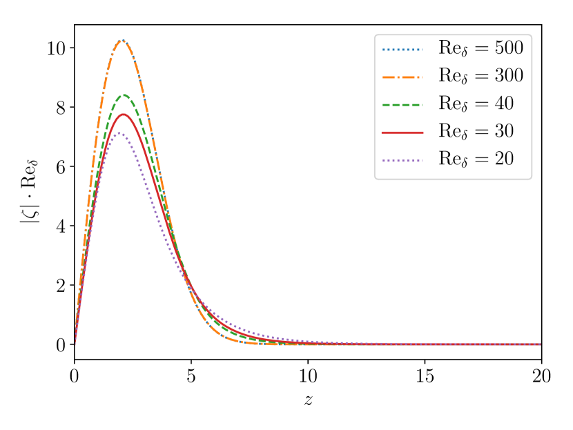
(b) $\zeta$

Figure 8: Initial condition for the streamwise streak with maximum amplification, $\max_{\beta,t_{0},t}G(\alpha=0,\beta,t_{0},t,\mbox{{Re}}_{\delta})$, for different Reynolds numbers.

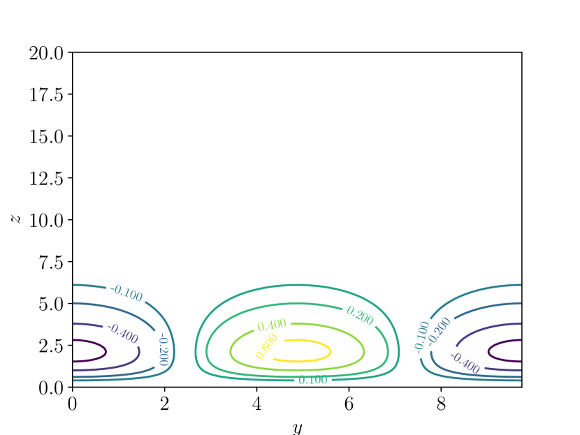
(a) $w(z,t_{0})\cdot\exp{\rm i}\beta y$

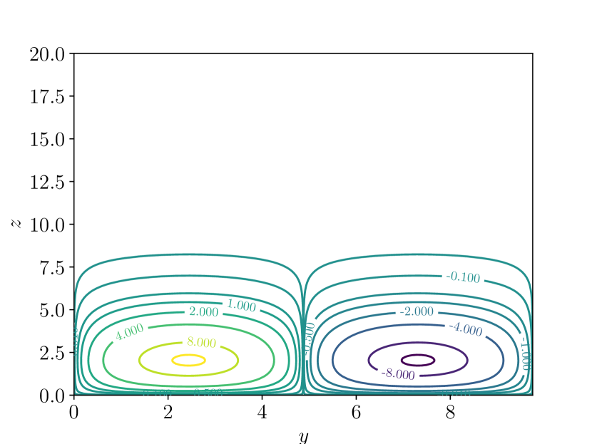
(b) $\zeta(z,t_{0})\cdot\exp{\rm i}\beta y\cdot\mbox{{Re}}$

Figure 9: Contour plots of the real part of $w(z,t_{0})\cdot\exp{\rm i}\beta y$ and the real part of $\zeta(z,t_{0})\cdot\exp{\rm i}\beta y\cdot\mbox{{Re}}$, which are the initial condition at $t_{0}$ for the optimal perturbation for the case $\mbox{{Re}}=500$, $\beta_{\max}=0.64$, $t_{0}=0.11$, $t=1.53$.

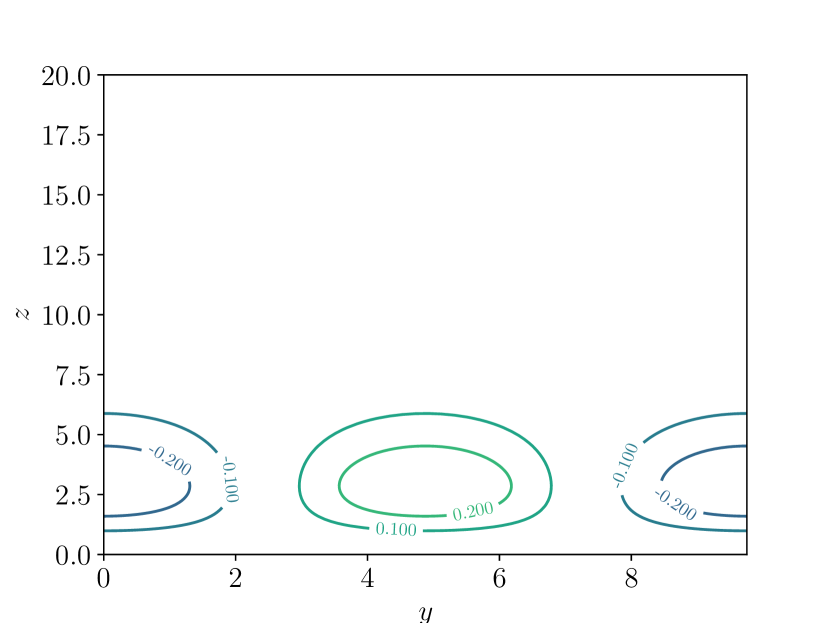
(a) $w(z,t)\cdot\exp{\rm i}\beta y$

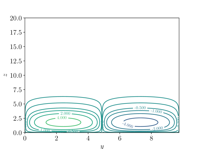
(b) $\zeta(z,t)\cdot\exp{\rm i}\beta y\cdot\mbox{{Re}}_{\delta}\cdot 10^{-3}$

Figure 10: Contour plots of the real part of $w(z,t)\cdot\exp{\rm i}\beta y$ and the real part of $\zeta(z,t)\cdot\exp{\rm i}\beta y\cdot\mbox{{Re}}\cdot 10^{-3}$, which are obtained by advancing the initial condition in figure 9 to time $t=1.53$ for the optimal perturbation for the case $\mbox{{Re}}=500$, $\beta_{\max}=0.64$, $t_{0}=0.11$.

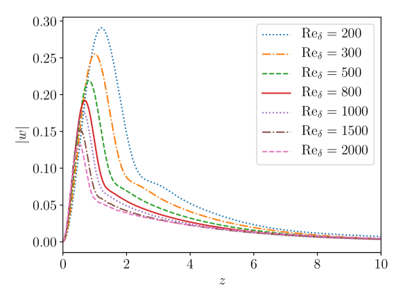
Figure 11: Initial condition $w$ for the two-dimensional perturbations with maximum amplification, $\max_{\alpha,t_{0},t}G(\alpha,\beta=0,t_{0},t,\mbox{{Re}}_{\delta})$, for different Reynolds numbers.

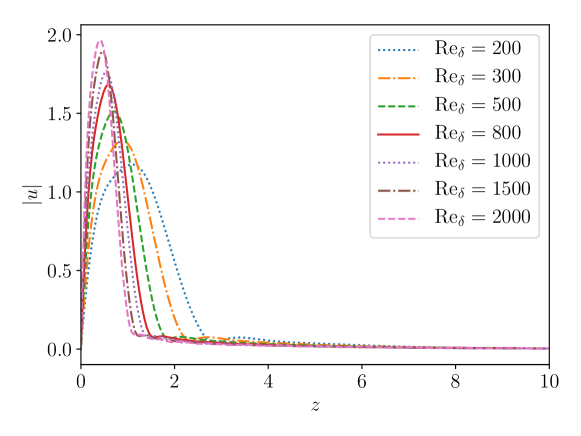
Figure 12: The horizontal component $u={\rm i}Dw/\alpha$ of the initial condition for two-dimensional perturbations with maximum amplification, $\max_{\alpha,t_{0},t}G(\alpha,\beta=0,t_{0},t,\mbox{{Re}}_{\delta})$, for different Reynolds numbers.

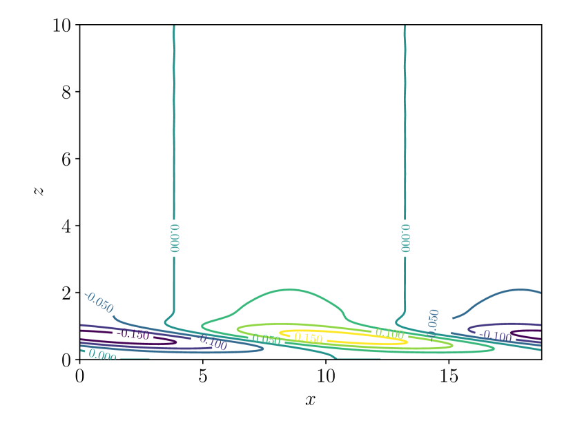
(a) $t_{0}=0.26$

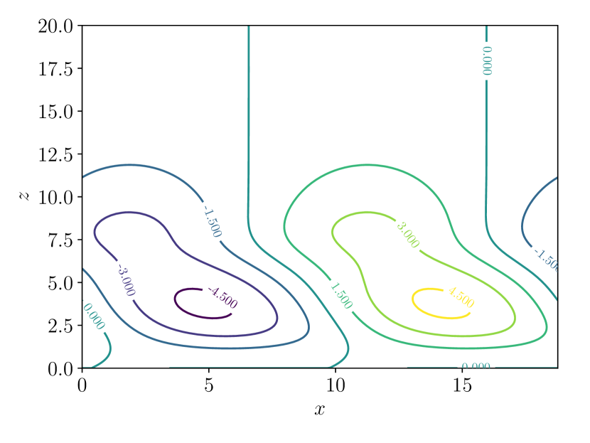
(b) $t=14.2$

Figure 13: Contour plots of the real part of $w\cdot\exp{\rm i}\alpha x$, at initial time $t_{0}=0.26$ and at $t=14.2$ ($w$ multiplied by $10^{-8}$), when it reaches its maximum amplification, for the optimal perturbation for the case $\mbox{{Re}}=1000$ with $\alpha_{\max}=0.33$.

4 Relation to previous results in the literature

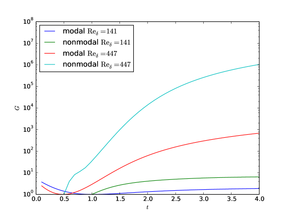
Figure 14: Amplification $G(\alpha=0.35,\beta=0,t_{0},t,\mbox{{Re}}_{\delta})$ of the nonmodal two-dimensional perturbation versus corresponding amplification of the modal Tollmien-Schlichting wave with $\alpha=0.35$ computed by means of the Orr-Sommerfeld equation, for $\mbox{{Re}}_{\delta}=141,447$. The initial time $t_{0}$ is taken from the minimum of the modal Tollmien-Schlichting waves.

A question which suggests itself immediately, is the relation between the present nonmodal stability analysis and the modal stability analyses performed previously in Blondeaux et al. (2012), Verschaeve & Pedersen (2014) and Sadek et al. (2015). Naturally, the amplifications of the optimal perturbations are expected to be larger than the corresponding ones of the modal Tollmien-Schlichting waves. This can be seen in figure 14, where we have solved the Orr-Sommerfeld equation for the present problem in a quasi-static fashion for the wave number $\alpha=0.35$ and Reynolds numbers $\mbox{{Re}}_{\delta}=141$ and $\mbox{{Re}}_{\delta}=447$. The amplification of the optimal perturbation can be several orders of magnitude larger than that of the corresponding modal Tollmien-Schlichting wave. On the other hand the main conclusions by Verschaeve & Pedersen (2014) are still supported by the present analysis. Although attempted by several experimental and direct numerical studies (Vittori & Blondeaux, 2008; Sumer et al., 2010; Ozdemir et al., 2013), a well defined transitional Reynolds number cannot be given for this flow. As also pointed out in the present analysis, depending on the characteristics of the external perturbations, such as length scale and intensity, the flow might transition to turbulence for different Reynolds numbers. Without control of the external perturbations, any experiment on the stability properties of this flow will hardly be repeatable. On the other hand, as we have shown above, a critical Reynolds number $\mbox{{Re}}_{A}$ can be defined for which the present flow switches from a monotonically stable to a non-monotonically stable flow. This critical Reynolds number has, however, little practical bearing.

Concerning the direct numerical simulations by Vittori & Blondeaux (2008, 2011) and Ozdemir et al. (2013), the present study gives an indication for the transition process happening via two-dimensional vortex rollers observed in their direct numerical simulations. In addition, we are able to answer the question raised by Ozdemir et al. (2013) about the possible mechanism of a by-pass transition. However, quantitative differences between the direct numerical results by Ozdemir et al. (2013) and the present ones exist. Ozdemir et al. (2013) introduced a random disturbance at $t_{0}=-\pi$ with different amplitudes in their simulations and monitored the evolution of the amplitude of these disturbances, cf. figure 10 in Ozdemir et al. (2013). From this figure, we see the characteristic kink of two-dimensional perturbations overtaking streamwise streaks appearing in their simulations only for $\mbox{{Re}}_{\delta}=2000$ and higher. If we compare this to the optimal perturbations with initial times $t_{0}=-4$ and $t_{0}=-2$ in figure 3, we see this kink developing already for a much lower Reynolds number, namely $\mbox{{Re}}_{\delta}=1000$, cf. figure 3d. The reasons for this discrepancy are unclear. Although Ozdemir et al. (2013) employed perturbation amplitudes with values up to 20 % of the base flow, which might trigger nonlinear effects, the acceleration region of the flow has a strong damping effect, such that the initial perturbation growth starting in the deceleration region is most likely governed by linear effects. We might, however, point out that, in order for a Navier-Stokes solver to capture the growth of two-dimensional perturbations correctly an extremely fine resolution in space and time is needed, as can be seen in Verschaeve & Pedersen (2014, Appendix A) for modal Tollmien-Schlichting waves. In particular, when the resolution requirements are not met, these perturbations tend to be damped instead of amplified. In this respect, it is interesting to note, that Vittori & Blondeaux (2008, 2011) found that regular vortex tubes appeared in their simulation for a Reynolds number around $\mbox{{Re}}_{\delta}=1000$ ($\mbox{{Re}}_{\rm Sumer}=5\cdot 10^{5}$), which corresponds relatively well with the present findings. However, it cannot be excluded that this is for the wrong reason, as a larger level of background noise resulting from, for example the numerical approximation error by their low order solver, might be present in their simulations.

The Reynolds number in the experiments by Liu et al. (2007) lies in the range $\mbox{{Re}}_{\delta}=72-143$ which is larger than $\mbox{{Re}}_{A}=18$. However, as can be seen from figure 3, the maximum amplification for these cases is around a factor of $30$. Therefore, without any induced disturbance, growth of streamwise streaks from background noise is probably not observable and has not been observed in Liu et al. (2007). On the other hand, in the experiments by Sumer et al. (2010) vortex rollers appeared in the range $630\leq\mbox{{Re}}_{\delta}<1000$. Assuming that the initial level of external perturbations in the experiments is higher than in the direct numerical simulations, the observation by Sumer et al. fits the present picture. However, for $\mbox{{Re}}_{\delta}>1000$, they observed the development of turbulent spots in the deceleration region of the flow. This is in contrast to the results by Ozdemir et al. (2013) of a $K$-type transition. The present analysis supports the finding of a transition process via the growth of two-dimensional perturbations. However, whether these nonmodal Tollmien-Schlichting waves break down via a $K$-type transition as in Ozdemir et al. (2013) or whether they break up randomly producing turbulent spots (Shaikh & Gaster, 1994; Gaster, 2016) is difficult to say from this primary instability analysis. In addition, more information on the initial disturbances in the experiments is needed to make any conclusions. Whereas random noise is applied in Vittori & Blondeaux (2008, 2011) and Ozdemir et al. (2013), the initial disturbance in Sumer et al. (2010) might stem from residual motion in their facility, exhibiting probably certain characteristics. Depending on these characteristics, other perturbations than the one showing optimal amplification, might induce secondary instability. In addition, it cannot be excluded that a completely different instability mechanism is at work in the experiments of Sumer et al. (2010). The focus in the present analysis is on the response to initial conditions and does not take into account any response to external forcing, which would be modeled by adding a source term to the equations (23) and (24). It is possible that the present flow system displays some sensitivity to certain frequencies of vibrations present in the experimental set-up altering the behavior of the system for larger Reynolds numbers. In particular, different perturbations, such as streamwise streaks, might be favored, leaving the possibility open that the turbulent spots, nevertheless, result from the break-down of streamwise streaks (Andersson et al., 2001; Brandt et al., 2004).

5 Conclusions

In the present treatise, a nonmodal stability analysis of the bottom boundary layer flow under solitary waves is performed. Two competing mechanism can be identified: Growing streamwise streaks and growing two-dimensional perturbations (nonmodal Tollmien-Schlichting waves). By means of an energy bound, it is shown that the present flow is monotonically stable for Reynolds numbers below $\mbox{{Re}}_{\delta}=18$ after which it turns non-monotonically stable, with streamwise streaks growing first. Two-dimensional perturbations display growth only for Reynolds numbers larger than $\mbox{{Re}}_{\delta}=38$. However, their maximum amplification overtakes that of streamwise streaks at $\mbox{{Re}}_{\delta}=170$. As for steady flows, the maximum amplification of streamwise streaks displays quadratic growth with $\mbox{{Re}}_{\delta}$ for the present unsteady flow. On the other hand, the maximum amplification of two-dimensional perturbations shows a near exponential growth with the Reynolds number in the deceleration region of the flow. Therefore, during primary instability, the dominant perturbations in the deceleration region of this flow are to be expected two-dimensional. This corresponds to the findings in the direct numerical simulations by Vittori & Blondeaux (2008) and Ozdemir et al. (2013) and in the experiments by Sumer et al. (2010) of growing two-dimensional vortex rollers in the deceleration region of the flow. However, further investigation of the secondary instability mechanism and of receptivity to external (statistical) forcing is needed in order to explain the subsequent break-down to turbulence in the boundary layer.

The boundary layer under solitary waves is a relatively simple model for a boundary layer flow with a favorable and an adverse pressure gradient. But just for this reason it allows to analyze stability mechanisms being otherwise shrouded in more complicated flows.

The implementation of the numerical method has been done using the open source libraries Armadillo (Sanderson & Curtin, 2016), FFTW (Frigo & Johnson, 2005) and GSL (Galassi et al., 2009). At this occasion, the first author would like to thank Caroline Lie for pointing out a mistake in Verschaeve & Pedersen (2014). In figures 20,22,24 and 26 in Verschaeve & Pedersen (2014), the frequency $\omega$ is incorrectly scaled. However, this does not affect any of the conclusions of the article. The first author apologizes for any inconvenience this might represent.

Appendix A Numerical implementation

A.1 Numerical implementation for the energy bound

We expand $\zeta$ and $w$ in equations (19-20) on the Shen-Legendre polynomials $\phi_{j}$ and $\psi_{j}$ for the Poisson and biharmonic operator, respectively, cf. (Shen, 1994):

$$\zeta=\sum\limits_{j=0}^{N-2}\zeta_{j}\phi_{j}(z)\quad w=\sum\limits_{j=0}^{N-4}w_{j}\psi_{j}(z),$$ (57)

where $N$ is the number of Legendre polynomials. The semi infinite domain $[0,\infty)$ is truncated at $h$, where $h$ is chosen large enough by numerical inspection. The basis functions $\phi_{j}$ and $\psi_{j}$ are linear combinations of Legendre polynomials, such that a total number of $N$ Legendre polynomials is used for each expansion in (57). The basis functions $\phi_{j}$ satisfy the homogeneous Dirichlet conditions, whereas $\psi_{j}$ honors the clamped boundary conditions. A Galerkin formulation is then chosen for the discrete system:

$$\left(\begin{array}[]{cc}\mathbf{A}&\mathbf{B}\\ \mathbf{B}^{T}&\mathbf{D}\end{array}\right)\left(\begin{array}[]{c}\mathbf{w}\\ \bm{\zeta}\end{array}\right)=\mu\left(\begin{array}[]{cc}\mathbf{E}&\mathbf{0}\\ \mathbf{0}&\mathbf{H}\end{array}\right)\left(\begin{array}[]{c}\mathbf{w}\\ \bm{\zeta}\end{array}\right).$$ (58)

The elements of the matrices are given by:

$$A_{ij} = \frac{1}{\mbox{{Re}}}\left\{\int\limits_{0}^{h}D^{2}\psi_{i}D^{2}\psi_{j}\,dz+2\left(\alpha^{2}+\beta^{2}\right)\int\limits_{0}^{h}D\psi_{i}D\psi_{j}\,dz+\left(\alpha^{2}+\beta^{2}\right)^{2}\int\limits_{0}^{h}\psi_{i}\psi_{j}\,dz\right\}$$ (59)

$$+\frac{{\rm i}\alpha}{2}\left\{\int\limits_{0}^{h}\psi_{i}\partial_{z}^{2}U_{\rm base}\psi_{j}\,dz+2\int\limits_{0}^{h}\psi_{i}\partial_{z}U_{\rm base}\partial_{z}\psi_{j}\,dz\right\}$$

$$B_{ij} = \frac{{\rm i}\beta}{2}\int\limits_{0}^{h}\psi_{i}\partial_{z}U_{\rm base}\phi_{j}\,dz$$ (60)

$$D_{ij} = \frac{1}{\mbox{{Re}}}\left\{\int\limits_{0}^{h}D\phi_{i}D\phi_{j}\,dz+\left(\alpha^{2}+\beta^{2}\right)\int\limits_{0}^{h}\phi_{i}\phi_{j}\,dz\right\}$$ (61)

$$2E_{ij} = -\int\limits_{0}^{h}D\psi_{i}D\psi_{j}\,dz-\left(\alpha^{2}+\beta^{2}\right)\int\limits_{0}^{h}\psi_{i}\psi_{j}\,dz$$ (62)

$$2H_{ij} = -\int\limits_{0}^{h}\phi_{i}\phi_{j}\,dz$$ (63)

For the verification and validation of the method, manufactured solutions have been used. In addition, the Reynolds numbers $\mbox{{Re}}_{A}$ and $\mbox{{Re}}_{B}$ for Stokes’ second problem have been computed, resulting into $\mbox{{Re}}_{A}=18.986$ and $\mbox{{Re}}_{B}=38.951$, corresponding well with the numbers $19.0$ and $38.9$ obtained by Davis & von Kerczek (1973, table 1).

A.2 Numerical implementation for the nonmodal analysis

The basis functions $\psi_{j}$ and $\phi_{j}$ for $w$ and $\zeta$ are in this case given by the Shen-Chebyshev polynomials, cf. Shen (1995), instead of the Shen-Legendre polynomials as before. This allows us to use the fast Fourier transform for computing derivatives. The equations (23-24) are written in discrete form as:

$$\frac{2}{\mbox{{Re}}_{\delta}}\left(\begin{array}[]{cc}\mathbf{L}^{\psi}&0\\ 0&\mathbf{M}^{\phi}\end{array}\right)\frac{d}{dt}\left(\begin{array}[]{c}\mathbf{w}\\ \bm{\zeta}\end{array}\right)=\left(\begin{array}[]{cc}\mathbf{L}^{OSE}&\mathbf{0}\\ \mathbf{L}^{C}&\mathbf{L}^{SC}\end{array}\right)\left(\begin{array}[]{c}\mathbf{w}\\ \bm{\zeta}\end{array}\right),$$ (64)

where the elements of the matrices are given by:

$$M_{ij}^{\psi} = \int\limits_{0}^{h}\psi_{i}\psi_{j}\,dz$$ (65)

$$G_{ij}^{\psi} = \int\limits_{0}^{h}\frac{d}{dz}\psi_{i}\frac{d}{dz}\psi_{j}\,dz$$ (66)

$$A^{\psi}_{ij} = \int\limits_{0}^{h}\frac{d^{2}}{dz^{2}}\psi_{i}\frac{d^{2}}{dz^{2}}\psi_{j}\,dz$$ (67)

$$M_{ij}^{\phi} = \int\limits_{0}^{h}\phi_{i}\phi_{j}\,dz$$ (68)

$$G^{\phi}_{ij} = \int\limits_{0}^{h}\frac{d}{dz}\phi_{i}\frac{d}{dz}\phi_{j}\,dz$$ (69)

$$P^{1}_{ij} = \int\limits_{0}^{h}\partial_{z}^{2}U_{\rm base}\psi_{i}\psi_{j}\,dz$$ (70)

$$P^{2}_{ij} = \int\limits_{0}^{h}U_{\rm base}\psi_{i}\left(D^{2}-(\alpha^{2}+\beta^{2})\right)\psi_{j}\,dz$$ (71)

$$P^{3}_{ij} = \int\limits_{0}^{h}U_{\rm base}\phi_{i}\phi_{j}\,dz$$ (72)

$$L^{\psi}_{ij} = -G_{ij}^{\psi}-(\alpha^{2}+\beta^{2})M_{ij}^{\psi}$$ (73)

$${L}_{ij}^{OSE} = {\rm i}\alpha P^{1}_{ij}-{\rm i}\alpha P^{2}_{ij}+\frac{1}{\rm Re}\left(A_{ij}^{\psi}+2\left(\alpha^{2}+\beta^{2}\right)G_{ij}^{\psi}+\left(\alpha^{2}+\beta^{2}\right)^{2}M_{ij}^{\psi}\right)$$ (74)

$${L}^{C}_{ik} = {\rm i}\beta\int\limits_{0}^{h}\partial_{z}U_{0}\phi_{i}\psi_{k}\,dz$$ (75)

$${L}^{SC}_{ij} = -{\rm i}\alpha P^{3}_{ij}+\frac{1}{\rm Re}\left(-G_{ij}^{\phi}-(\alpha^{2}+\beta^{2})M_{ij}^{\phi}\right)$$ (76)

For the Shen-Chebyshev polynomials, $\mathbf{L}^{\psi}$ and $\mathbf{M}^{\phi}$ are sparse banded matrices. Therefore, the system (64) can be efficiently advanced in time, allowing us to compute the evolution matrix $\mathbf{X}(t,t_{0})$ for a wide range of parameters. The amplification $G$, equation (26), for the discrete case can then be computed as suggested in Trefethen et al. (1993); Schmid & Henningson (2001); Schmid (2007). We write

$$\mathbf{q}=\left(\begin{array}[]{c}\mathbf{w}\\ \bm{\zeta}\end{array}\right),$$ (77)

and note that the energy $E$, equation (25), in the discrete case is given by:

$$E=\mathbf{q}^{*}\mathbf{W}\mathbf{q},$$ (78)

where

$$\mathbf{W}=\frac{1}{2}\left(\begin{array}[]{cc}\frac{1}{k^{2}}\mathbf{G}^{\psi}+\mathbf{M}^{\psi}&0\\ 0&\frac{1}{k^{2}}\mathbf{M}^{\phi}\end{array}\right).$$ (79)

Matrices $\mathbf{G}^{\psi}$, $\mathbf{M}^{\psi}$ and $\mathbf{M}^{\phi}$ are defined in equations (66), (65) and (68), respectively. The Cholesky factorization of $\mathbf{W}$ is given by:

$$\mathbf{F}^{T}\mathbf{F}=\mathbf{W}.$$ (80)

The coefficients $\mathbf{q}(t)$ at time $t$ can be obtained by means of the evolution matrix $\mathbf{X}$:

$$\mathbf{q}(t)=\mathbf{X}(t,t_{0})\mathbf{q}_{0},$$ (81)

where $\mathbf{q}_{0}$ is the initial condition at $t_{0}$. From this it follows that $\mathbf{X}(t_{0},t_{0})$ reduces to the identity matrix. The amplification $G$ can then be computed by

$$G(\alpha,\beta,t_{0},t,\mbox{{Re}}_{\delta}) = \max_{\mathbf{q}_{0}}\frac{\mathbf{q}(t)^{\dagger}\mathbf{W}\mathbf{q}(t)}{\mathbf{q}_{0}^{\dagger}\mathbf{W}\mathbf{q}_{0}}$$ (82)

$$= \max_{\mathbf{q}_{0}}\frac{\mathbf{q}_{0}^{\dagger}\mathbf{X}^{\dagger}\mathbf{W}\mathbf{X}\mathbf{q}_{0}}{\mathbf{q}_{0}^{\dagger}\mathbf{W}\mathbf{q}_{0}}$$ (83)

$$= \max_{\mathbf{b}}\frac{\mathbf{b}^{\dagger}\mathbf{F}^{-T}\mathbf{X}^{\dagger}\mathbf{W}\mathbf{X}\mathbf{F}^{-1}\mathbf{b}}{\mathbf{b}^{\dagger}\mathbf{b}}$$ (84)

$$= \left|\left|\mathbf{F}\mathbf{X}\mathbf{F}^{-1}\right|\right|^{2},$$ (85)

where the matrix norm $\left|\left|\mathbf{F}\mathbf{X}\mathbf{F}^{-1}\right|\right|$ is given by the maximum singular value of $\mathbf{F}\mathbf{X}\mathbf{F}^{-1}$, cf. Trefethen et al. (1993); Schmid & Henningson (2001); Schmid (2007).

The present method consists of two steps. First, the evolution matrix $\mathbf{X}$ needs to be computed by solving equation (64) with the identity matrix as initial condition at time $t_{0}$. Then the amplification $G$ can be computed using $\mathbf{X}$. In order to verify the well functioning of the present time integration, the following manufactured solution has been used:

$$w=\cos(\omega_{1}t)\sin^{2}(5\pi z)\quad\zeta=\cos(\omega_{2}t)\sin(3\pi z)\quad U_{\rm base}=\cos(\omega_{3}t)\left(1-\exp\left(-2z\right)\right).$$ (86)

A forcing term is defined by the resulting term, when injecting the above solution into equations (23) and (24). Equations (64) are advanced by means of the adaptive Runge-Kutta-Cash-Karp-54 time integrator included in the boost library. The absolute and relative error of the time integration are set to $10^{-10}$. For verification, we use the above manufactured solution with the following parameter values:

$$\mbox{{Re}}_{\delta}=123\quad\alpha=0.3\quad\beta=0.234\quad h=1\quad\omega_{1}=1.234\quad\omega_{2}=1.123\quad\omega_{3}=0.4567\quad t_{0}=0,$$ (87)

and compare reference and numerical solution by computing a mean error on the Chebyshev knots. The behavior of the error for increasing $N$ is displayed in figure 15. We observe that the error displays exponential convergence until approximately $10^{-9}$, when the error contribution due to the time integration becomes dominant. In addition, the analytic solution of the energy of this problem can be used to verify parts of the amplification computation (results not shown).

For validation purposes, the case of transient growth for Poiseuille flow with a Reynolds number $\mbox{{Re}}=1000$ and $\alpha=1$ in Schmid (2007) has been computed by means of the present method for $N=65$. As can be seen from figure 16, the results by the present method correspond well to the data digitized from figure 3 in Schmid (2007).

Furthermore, the validation with an unsteady base flow is performed by means of Stokes second problem whose base flow is given by

$$U_{\rm base}=\exp(-z)\cos\left(\frac{2}{\mbox{{Re}}_{\delta}}t-z\right).$$ (88)

The results in Luo & Wu (2010) define a test case for the present method. In Luo & Wu (2010), the temporal evolution of eigenmodes of the Orr-Sommerfeld equation for $t_{0}=0$ is investigated. They consider three cases defined by $\mbox{{Re}}_{\delta}=1560$, $1562.8$ and $1566$ and $\alpha=0.3$ and $\beta=0$. As initial condition, the eigenmodes corresponding to the following eigenvalues $\omega_{\rm OSE}$ for each $\mbox{{Re}}_{\delta}$ are used:

$$\begin{array}[]{l|r}\mbox{{Re}}_{\delta}&\omega_{\rm OSE}\\ \hline\cr 1560&-0.004847-0.196045{\rm i}\\ 1562.8&-0.00482994-0.196076{\rm i}\\ 1566&-0.00481052-0.196111{\rm i}\end{array}$$

As a main result from the investigation in Luo & Wu (2010), the maximum amplitude of the perturbation for $\mbox{{Re}}_{\delta}=1560$ decreases from cycle to cycle, whereas for $\mbox{{Re}}_{\delta}=1562.8$ the maximum amplitude displays almost no growth from cycle to cycle. However, for $\mbox{{Re}}_{\delta}=1566$, the maximum amplitude increases from cycle to cycle. This can also be observed when using the present method, cf. figure 17, where we have used $N=97$. The amplitude is in our case defined by the ratio between the perturbation energy at time $t$ and at time $t_{0}=0$. Luo & Wu (2010) defined the amplitude differently, namely by the first coefficient of the expansion of the perturbation on all Orr-Sommerfeld modes. Therefore, the exact numerical values in figure 17 and in figure 7 in Luo & Wu (2010) are not comparable. When comparing the growth rate $\omega$ of the present perturbation, given by:

$$\omega=\frac{1}{E}\frac{dE}{dt}$$ (89)

with the growth rate given by the real part of the eigenvalue resulting from the Orr-Sommerfeld equation for the case $\mbox{{Re}}_{\delta}=1566$, we confirm the observation by (Luo & Wu, 2010, figure 10) that during one cycle the growth rate is relatively well approximated by the Orr-Sommerfeld solution. In addition, the growth rate taken from figure 10 in Luo & Wu (2010) by digitization follows closely the present one, even if the definition of the amplitude is a different one, cf. figure 18.

Returning to the present flow, we shall consider the case

$$\mbox{{Re}}_{\delta}=1000\quad\alpha=0.6\quad\beta=0.14\quad h=30\quad t_{0}=0\quad t=6,$$ (90)

for determining the discretization parameters. Before solving the nonmodal equations (64), the base flow solution needs to be generated. This is done by numerically solving the boundary layer equations (3-6), applying the same discretization techniques as for the nonmodal equations (23-24). The present boundary layer solver has been verified by comparison to the solution obtained by means of the integral formula in Liu et al. (2007). An important ingredient in the numerical solution of the boundary layer equations (3-6) is the choice of a finite value $t_{-\infty}$ for imposing the boundary condition (5). As the outer flow dies off exponentially towards $t\rightarrow\pm\infty$, we choose $t_{-\infty}=-8$ and $t_{-\infty}=-12$ as starting point. For these values the magnitude of the outer flow amounts to $U_{\rm outer}(t_{-\infty}=-8)=4.50141\cdot 10^{-7}$ and $U_{\rm outer}(t_{-\infty}=-12)=1.51005\cdot^{-10}$, respectively. Choosing $N=129$, we solve the above nonmodal example problem, equation (90), for $U_{\rm base}$ computed with $t_{-\infty}=-8$ and $t_{-\infty}=-12$. The resulting amplification $G$ is given by:

$$G(0.6,0.14,0,6,1000)=1.11855\cdot 10^{9} \mbox{for}\quad t_{-\infty}=-8$$ (91)

$$G(0.6,0.14,0,6,1000)=1.11869\cdot 10^{9} \mbox{for}\quad t_{-\infty}=-12.$$ (92)

Choosing $t_{-\infty}=-12$ and varying the number of Chebyshev polynomials $N$, we observe the following values for G:

$$\begin{array}[]{r|l}N&G(0.6,0.14,0,6,1000)\\ \hline\cr 33&2.22803\cdot 10^{13}\\ 49&3.51768\cdot 10^{8}\\ 65&1.13902\cdot 10^{9}\\ 97&1.11865\cdot 10^{9}\\ 129&1.11869\cdot 10^{9}\end{array}$$

For the simulations in section 3, computations with $N=97$ and $N=129$ have been performed to ensure that the results are accurate.

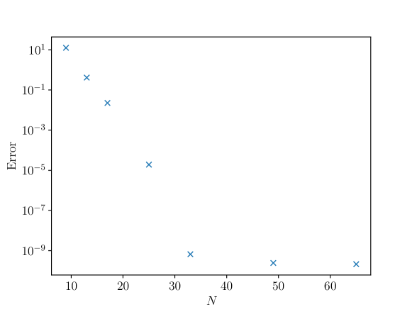
Figure 15: Error convergence of the manufactured problem given by equation 86.

Figure 16: Amplification $G(\alpha=1.,\beta=0,t_{0}=0.,t,\mbox{{Re}}=1000.)$ of the nonmodal perturbation for Poiseuille flow. The present results collapse onto the data from figure 3 in Schmid (2007).

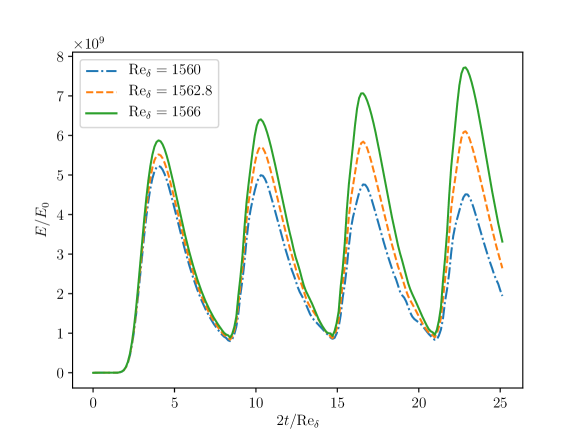
Figure 17: Temporal evolution of the amplitude $E/E_{0}$ when advancing the Orr-Sommerfeld eigenmode at time $t_{0}=0$ forward in time with the present method.

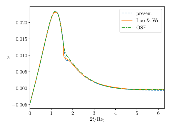
Figure 18: Growth rate of the perturbation when advancing the Orr-Sommerfeld eigenmode at time $t_{0}=0$ forward in time with the present method.

Appendix B Scaling of the initial condition for streamwise streaks

For streamwise streaks ($\alpha=0$), we have the governing equations given by equations (28) and (29). We shall first find the general solution of $\tilde{\zeta}$.

The sine transform of $\tilde{\zeta}$ is defined as:

$$\Theta(\gamma,t)=\int\limits_{0}^{\infty}\tilde{\zeta}\sin(\gamma z)\,dz$$ (93)

Taking the sine transform of equation (29), gives us:

$$\frac{\partial}{\partial t}\Theta+\frac{1}{2}\left(\gamma^{2}+\beta^{2}\right)\Theta-F=0,$$ (94)

where

$$F(\gamma,t)={\rm i}\beta\int\limits_{0}^{\infty}wDU_{\rm base}\sin(\gamma z)\,dz.$$ (95)

Solving equation (94) gives us for $\Theta$:

$$\Theta(\gamma,t)=\left(\Theta(\gamma,0)+\int\limits_{0}^{t}\frac{F(\gamma,\tau)}{e^{-\frac{1}{2}\left(\beta^{2}+\gamma^{2}\right)\tau}}\,d\tau\right)e^{-\frac{1}{2}\left(\beta^{2}+\gamma^{2}\right)t}.$$ (96)

The general solution of $\tilde{\zeta}$ can thus be written as:

$$\tilde{\zeta} = \frac{2}{\pi}\int\limits_{0}^{\infty}\Theta(\gamma,0)e^{-\frac{1}{2}\left(\beta^{2}+\gamma^{2}\right)t}\sin(\gamma z)\,d\gamma$$ (97)

$$+\frac{2}{\pi}\int\limits_{0}^{\infty}e^{-\frac{1}{2}\left(\beta^{2}+\gamma^{2}\right)t}\int\limits_{t_{0}}^{t}\frac{F(\gamma,\tau)}{e^{-\frac{1}{2}\left(\beta^{2}+\gamma^{2}\right)\tau}}\,d\tau\sin(\gamma z)\,d\gamma.$$

Motivated by the findings in section (3.2.2), we shall assume that in the asymptotic limit $\mbox{{Re}}_{\delta}\rightarrow\infty$, the initial condition of $w$ and $\tilde{\zeta}$ can approximately be written as:

$$w=w_{m}(\mbox{{Re}}_{\delta})\hat{w}(z,t_{0})\quad\tilde{\zeta}=\zeta_{m}(\mbox{{Re}}_{\delta})\hat{\zeta}(z,t_{0}),$$ (98)

where only the coefficients $w_{m}$ and $\zeta_{m}$ depend on $\mbox{{Re}}_{\delta}$. Subsequently, using equation (97), we can write $w$ and $\tilde{\zeta}$ as:

$$\tilde{\zeta} = \zeta_{m}a(z,t)+w_{m}b(z,t),$$ (99)

$$w = w_{m}c(z,t),$$ (100)

where $a$, $b$ and $c$ are some functions of $z$ and $t$, with $b(z,t_{0})=0$. The energy $E=E_{w}+E_{\zeta}$, equation (25), is then given by:

$$E_{w}(t) = w_{m}^{2}\frac{1}{2}\int\limits_{0}^{\infty}\frac{1}{\beta^{2}}|Dc|^{2}+|c|^{2}\,dz,$$ (101)

$$E_{\zeta}(t) = \frac{1}{2}\frac{\mbox{{Re}}_{\delta}^{2}}{4}\int\limits_{0}^{\infty}\frac{1}{\beta^{2}}\left(\zeta_{m}^{2}a^{2}+2\zeta_{m}w_{m}ab+w_{m}^{2}b^{2}\right)\,dz.$$ (102)

We can thus write:

$$E_{w}(t_{0}) = w_{m}^{2}A_{0},$$ (103)

$$E_{w}(t) = w_{m}^{2}A_{1},$$ (104)

$$E_{\zeta}(t_{0}) = \mbox{{Re}}_{\delta}^{2}\zeta_{m}^{2}B_{0},$$ (105)

$$E_{\zeta}(t) = \mbox{{Re}}_{\delta}^{2}\left(\zeta_{m}^{2}B_{1}+2\zeta_{m}w_{m}B_{2}+w_{m}^{2}B_{3}\right),$$ (106)

where $A_{0}$, $A_{1}$, $B_{0}$, $B_{1}$, $B_{2}$ and $B_{3}$ are independent of $\mbox{{Re}}_{\delta}$. The normalization constraint for the initial condition reads:

$$E_{w}(t_{0})+E_{\zeta}(t_{0})=w_{m}^{2}A_{0}+\mbox{{Re}}_{\delta}^{2}\zeta_{m}^{2}B_{0}=1,$$ (107)

From which we find:

$$w_{m}^{2}=\frac{1}{A_{0}}\left(1-\mbox{{Re}}_{\delta}^{2}B_{0}\zeta_{m}^{2}\right)$$ (108)

As the right hand side needs to be positive for all $\mbox{{Re}}_{\delta}$, this motivates the following ansatz for $\zeta_{m}$ in the limit of $\mbox{{Re}}_{\delta}\rightarrow\infty$:

$$\zeta_{m}=\frac{d}{\mbox{{Re}}_{\delta}^{\theta}},$$ (109)

where $\theta\geq 1$ and $d$ some constant. For the energy at time $t$, we can write:

$$E(t) = w_{m}^{2}A_{1}+\mbox{{Re}}_{\delta}^{2}\left(\zeta_{m}^{2}B_{1}+2\zeta_{m}w_{m}B_{2}+w_{m}^{2}B_{3}\right)$$ (110)

$$= \frac{1}{{A_{0}}}\Big{(}2d\,{{\mbox{{Re}}_{\delta}}}^{-\theta+2}\sqrt{A_{0}}\,{B_{2}}\,\sqrt{{{\left({{\mbox{{Re}}_{\delta}}}^{2\,\theta}-{B_{0}}\,{{\mbox{{Re}}_{\delta}}}^{2}{d}^{2}\right){{\mbox{{Re}}_{\delta}}}^{-2\,\theta}}}}$$

$$\quad\quad+{d}^{2}\left({A_{0}}\,{B_{1}}-{A_{1}}\,{B_{0}}\right){{\mbox{{Re}}_{\delta}}}^{2-2\,\theta}-{{\mbox{{Re}}_{\delta}}}^{-2\,\theta+4}{B_{0}}\,{B_{3}}\,{d}^{2}+{B_{3}}\,{{\mbox{{Re}}_{\delta}}}^{2}+{A_{1}}\Big{)}.$$

As the energy is maximum for the optimal perturbation, we must have

$$\frac{\partial E}{\partial\theta}=0.$$ (112)

Solving this equation for $\theta$ gives us four solutions

$$\theta_{1,2,3,4}=1/2\,{\frac{1}{\ln\left({\mbox{{Re}}_{\delta}}\right)}\left(-\ln\left(2\right)+2\,\ln\left(\pm{\frac{d}{{B_{2}}}\sqrt{\frac{F_{\pm}}{A_{0}}}}\right)\right)},$$ (113)

where

$$F_{\pm} = \pm\sqrt{D}+\left({{B_{3}}}^{2}{{\mbox{{Re}}_{\delta}}}^{4}+2\,{A_{1}}\,{B_{3}}\,{{\mbox{{Re}}_{\delta}}}^{2}+{{A_{1}}}^{2}\right){{B_{0}}}^{2}$$ (114)

$$+\left(\left(-2\,{B_{1}}\,{B_{3}}+4\,{{B_{2}}}^{2}\right){{\mbox{{Re}}_{\delta}}}^{2}-2\,{A_{1}}\,{B_{1}}\right){A_{0}}\,{B_{0}}+{{A_{0}}}^{2}{{B_{1}}}^{2}$$

$$D = \left(\left(-{B_{3}}\,{{\mbox{{Re}}_{\delta}}}^{2}-{A_{1}}\right){B_{0}}+{A_{0}}\,{B_{1}}\right)^{2}$$

$$\left(\left({B_{3}}\,{{\mbox{{Re}}_{\delta}}}^{2}+{A_{1}}\right)^{2}{{B_{0}}}^{2}-2\,{A_{0}}\,\left(\left({B_{1}}\,{B_{3}}-2\,{{B_{2}}}^{2}\right){{\mbox{{Re}}_{\delta}}}^{2}+{A_{1}}\,{B_{1}}\right){B_{0}}+{{A_{0}}}^{2}{{B_{1}}}^{2}\right)$$

Taking the limit $\mbox{{Re}}_{\delta}\rightarrow\infty$, we obtain:

$$\lim_{\mbox{{Re}}_{\delta}\rightarrow\infty}\theta_{i}=2\quad\mbox{for}\quad i=1,2,3,4.$$ (116)

From this it follows, that for $\mbox{{Re}}_{\delta}>>1$, we have approximately

$$\tilde{\zeta}(z,t_{0})\propto\frac{1}{\mbox{{Re}}_{\delta}^{2}},$$ (117)

from which relation (52) can directly be obtained.

References

- Andersson et al. (2001) Andersson, P. , Brandt, L. , Bottaro, A. & Henningson, D. S. 2001 On the breakdown of boundary layer streaks. Journal of Fluid Mechanics 428, 29–60.
- Benjamin (1966) Benjamin, T. B. 1966 Internal waves of finite amplitude and permanent form. Journal of Fluid Mechanics 25, 241–270.
- Bertolotti et al. (1992) Bertolotti, F. , Herbert, T. & Spalart, P. 1992 Linear and nonlinear stability of the Blasius boundary layer. Journal of Fluid Mechanics 242, 441–474.
- Biau (2016) Biau, D. 2016 Transient growth of perturbations in stokes oscillatory flows. Journal of Fluid Mechanics 794, 10.
- Blondeaux et al. (2012) Blondeaux, P. , Pralits, J. & Vittori, G. 2012 Transition to turbulence at the bottom of a solitary wave. Journal of Fluid Mechanics 709, 396–407.
- Brandt et al. (2004) Brandt, L. , Schlatter, P. & Henningson, D. S. 2004 Transition in boundary layers subject to free-stream turbulence. Journal of Fluid Mechanics 517, 167–198.
- Butler & Farrell (1992) Butler, K. M. & Farrell, B. F. 1992 Three-dimensional optimal perturbations in viscous shear flow. Physics of Fluids A 4, 1637–1650.
- Carr & Davies (2006) Carr, M. & Davies, P. A. 2006 The motion of an internal solitary wave of depression over a fixed bottom boundary in a shallow, two-layer fluid. Physics of Fluids 18, 016601–10.
- Carr & Davies (2010) Carr, M. & Davies, P. A. 2010 Boundary layer flow beneath an internal solitary wave of elevation. Physics of Fluids 22, 026601–1–8.
- Corbett & Bottaro (2000) Corbett, P. & Bottaro, A. 2000 Optimal perturbations for boundary layers subject to stream-wise pressure gradient. Physics of Fluids 12 (1), 120–130.
- Corbett & Bottaro (2001) Corbett, P. & Bottaro, A. 2001 Optimal linear growth in swept boudary layers. Journal of Fluid Mechanics 435, 1–23.
- Davis & von Kerczek (1973) Davis, S. H. & von Kerczek, C. 1973 A reformulation of energy stability theory. Archive for Rational Mechanics and Analysis pp. 112–117.
- Ellingsen & Palm (1975) Ellingsen, T. & Palm, E. 1975 Hydrodynamic stability. Physics of Fluids 18, 487.
- Fenton (1972) Fenton, J. 1972 A ninth-order solution for the solitary wave. Journal of Fluid Mechanics 53, 257–271.
- Frigo & Johnson (2005) Frigo, M. & Johnson, S. G. 2005 The design and implementation of FFTW3. In Proceedings of the IEEE, , vol. 93, pp. 216–231.
- Galassi et al. (2009) Galassi, M. , Davies, J. , Theiler, B. , Gough, B. , Jungman, G. , Alken, P. , Booth, M. & Rossi, F. 2009 GNU Scientific Library Reference Manual. Network Theory Ltd.
- Gaster (2016) Gaster, M. 2016 Boundary layer transition initiated by a random excitation. In Book of Abstracts International Congress of Theoretical and Applied Mechanics.
- Grimshaw (1971) Grimshaw, R. 1971 The solitary wave in water of variable depth. part 2. Journal of Fluid Mechanics 46, 611–622.
- Gustavsson (1991) Gustavsson, L. H. 1991 Energy growth of three-dimensional disturbances in plane Poiseuille flow. Journal of Fluid Mechanics 224, 241–260.
- Herbert (1988) Herbert, T. 1988 Secondary instability of boundary layers. Annual Review of Fluid Mechanics 20, 487–526.
- Jimenez (2013) Jimenez, J. 2013 How linear is wall-bounded turbulence? Physics of Fluids 25, 110814–1–19.
- Joseph (1966) Joseph, D. D. 1966 Nonlinear stability of the boussinesq equations by the method of energy. Archive for Rational Mechanics and Analysis 22, 163.
- von Kerczek & Davis (1974) von Kerczek, C. & Davis, S. H. 1974 Linear stability theory of oscillatory stokes layers. Journal of Fluid Mechanics 62, 753–773.
- Levin & Henningson (2003) Levin, O. & Henningson, D. S. 2003 Exponential vs algebra growth and transition prediction in boundary layer flow. Flow, Turbulence and Combustion 70, 183–210.
- Liu & Orfila (2004) Liu, P. L.-F. & Orfila, A. 2004 Viscous effects on transient long-wave propagation. Journal of Fluid Mechanics 520, 83–92.
- Liu et al. (2007) Liu, P. L.-F. , Park, Y. S. & Cowen, E. A. 2007 Boundary layer flow and bed shear stress under a solitary wave. Journal of Fluid Mechanics 574, 449–463.
- Luchini & Bottaro (2014) Luchini, P. & Bottaro, A. 2014 Adjoint equations in stability analysis. Annual Review of Fluid Mechanics 46, 493–517.
- Luo & Wu (2010) Luo, J. & Wu, X. 2010 On the linear instability of a finite stokes layer: Instantaneous versus floquet modes. Physics of Fluids 22, 1–13.
- Miles (1980) Miles, J. W. 1980 Solitary waves. Annual Review of Fluid Mechanics 12, 11–43.
- Ozdemir et al. (2013) Ozdemir, C. E. , Hsu, T.-J. & Balachandar, S. 2013 Direct numerical simulations of instability and boundary layer turbulence under a solitay wave. Journal of Fluid Mechanics 731, 545–578.
- Park et al. (2014) Park, Y. S. , Verschaeve, J. C. G. , Pedersen, G. K. & Liu, P. L.-F. 2014 Corrigendum and addendum for boundary layer flow and bed shear stress under a solitary wave. Journal of Fluid Mechanics 753, 554–559.
- Sadek et al. (2015) Sadek, M. M. , Parras, L. , Diamessis, P. J. & Liu, P. L.-F. 2015 Two-dimensional instability of the bottom boundary layer under a solitary wave. Physics of Fluids 27, 044101–1–25.
- Sanderson & Curtin (2016) Sanderson, C. & Curtin, R. 2016 Armadillo: a template-based C++ library for linear algebra. Journal of Open Source Software 1, 26.
- Schmid (2007) Schmid, P. J. 2007 Nonmodal stability theory. Annual Review of Fluid Mechanics 39, 129–162.
- Schmid & Henningson (2001) Schmid, P. J. & Henningson, D. S. 2001 Stability and Transition in Shear Flows. New York: Springer-Verlag.
- Shaikh & Gaster (1994) Shaikh, F. N. & Gaster, M. 1994 The non-linear evolution of modulated waves in a boundary layer. Journal of Engineering Mathematics 28, 55–71.
- Shen (1994) Shen, J. 1994 Efficient spectral-galerkin method i. direct solvers for the second and fourth order equations using legendre polynomials. Siam Journal of Scientific Coputing 15, 1489–1505.
- Shen (1995) Shen, J. 1995 Efficient spectral-galerkin method ii. direct solvers of second fourth order equations by using chebyshev polynomials. SIAM Journal of Scientific Computing 16 (1), 74–87.
- Shuto (1976) Shuto, N. 1976 Transformation of nonlinear long waves. In Proceedings of 15th Conference on Coastal Enginearing.
- Sumer et al. (2010) Sumer, B. M. , Jensen, P. M. , Sørensen, L. B. , Fredsøe, J. , Liu, P. L.-F. & Carstensen, S. 2010 Coherent structures in wave boundary layers. part 2. solitary motion. Journal of Fluid Mechanics 646, 207–231.
- Tanaka et al. (2011) Tanaka, H. , Winarta, B. , Suntoyo & Yamaji, H. 2011 Validation of a new generation system for bottom boundary layer beneath solitary wave. Coastal Engineering 59, 46–56.
- Trefethen et al. (1993) Trefethen, L. N. , Trefethen, A. E. , Reddy, S. C. & Driscoll, T. A. 1993 Hydrodynamic stability witwith eigenvalues. Science 261, 578–584.
- Verschaeve & Pedersen (2014) Verschaeve, J. C. G. & Pedersen, G. K. 2014 Linear stability of boundary layers under solitary waves. Journal of Fluid Mechanics 761, 62–104.
- Vittori & Blondeaux (2008) Vittori, G. & Blondeaux, P. 2008 Turbulent boundary layer under a solitary wave. Journal of Fluid Mechanics 615, 433–443.
- Vittori & Blondeaux (2011) Vittori, G. & Blondeaux, P. 2011 Characteristics of the boundary layer at the bottom of a solitary wave. Coastal Engineering 58, 206–213.