The shear viscosity of two-flavor crystalline color superconducting quark matter

Abstract

We present the first calculation of the shear viscosity for two-flavor plane wave (FF) color superconducting quark matter. This is a member of the family of crystalline color superconducting phases of dense quark matter that may be present in the cores of neutron stars. The paired quarks in the FF phase feature gapless excitations on surfaces of crescent shaped blocking regions in momentum space and participate in transport. We calculate their contribution to the shear viscosity. We note that they also lead to dynamic screening of transverse $t^{1}$, $t^{2}$, $t^{3}$ gluons which are undamped in the $2{\rm{SC}}$ phase. The exchange of these gluons is the most important mechanism of the scattering of the paired quarks. We find that the shear viscosity of the paired quarks is roughly a factor of $100$ smaller compared to the shear viscosity of unpaired quark matter. Our results may have implications for the damping of $r-$modes in rapidly rotating, cold neutron stars.

I Introduction

The discovery of neutron stars with masses close to $2M_{\odot}$ Demorest et al. (2010); Antoniadis et al. (2013), (see Ref. Ozel and Freire (2016) for a recent review), has provided a strong constraint on the equation of state of matter in neutron stars Page and Reddy (2006); Ozel et al. (2010); Y Potekhin (2010); Lattimer (2012); Prakash (2015) ruling out large parameter spaces in various models of dense matter. (For quark matter see Ref. Ranea-Sandoval et al. (2016).) Refinements in the measurements on the radii of neutron stars provide additional constraints on the equation of state Steiner et al. (2013); Lattimer and Steiner (2014).

In addition to analyzing constraints on the equation of state, characterising the nature of the phases of matter in neutron stars will require observationally constraining the transport properties of neutron stars. These observations can help eliminate models of dense matter inconsistent with the data Page and Reddy (2006). Transport properties are sensitive to the spectrum of excitations above the equilibrium state (which is essentially the ground state because the temperatures of neutron stars are much smaller than the other relevant energy scales). These excitations can differ substantially for phases with similar equations of state.

For example, the short time (time scales of many days) thermal evolution already constrains the thermal conductivity and the specific heat of matter in the neutron star crust (Chamel and Haensel (2008); Page and Reddy (2012) and references therein). Neutrino cooling on much longer time scales ($10^{5}$ years) depends on the phase of matter inside the cores (see Ref. Pethick (1992); Yakovlev et al. (2001, 2003) for a review). A neutron star of mass around $1.4M_{\odot}$, with a core of only protons, electrons and neutrons cools “slowly”. The presence of condensates, strange particles, or unpaired quark matter in the cores, leads to “fast” cooling. One hopes that observations of the temperatures and the ages of neutron stars will be able to tell us whether neutron star cores feature such exotic phases.

A set of observables sensitive to the viscosity of matter in the cores of neutron stars are the spin frequencies, temperatures, and the spin-down rates of fast rotating neutron stars Alford and Schwenzer (2014). In the absence of viscous damping, the fluid in rotating neutron stars is Andersson (1998); Andersson and Kokkotas (1998) unstable to a mode which couples to gravity which radiates away the angular momentum of the star. If the mode grows the neutron stars are expected to spin down rapidly. This is the famous $r$-mode instability.

The connection between the viscosity and the spin observables is subtle because it depends on the amplitude Lindblom et al. (2001); Alford et al. (2012a) (determined by non-linear physics) at which the $r$-mode saturates if the star winds up in the regime where the $r$-mode is unstable in the linear approximation. But the essence of the connection can be understood easily Andersson (1998); Andersson and Kokkotas (1998); Alford et al. (2012b) by ignoring the saturation dynamics. In this regime the amplitude of the mode changes with time as,

$${\cal{A}}e^{-(\Gamma_{\rm{GW}}+\Gamma_{\rm{Bulk}}+\Gamma_{\rm{Shear}})t}$$ (1)

where $\Gamma_{\rm{GW}}<0$. $\Gamma_{\rm{Bulk}}$ and $\Gamma_{\rm{Shear}}$ are both positive and depend on the bulk and shear viscosities throughout the star and therefore depend on the phase of matter in the core and the temperature of the star. The magnitude of $\Gamma_{\rm{GW}}$ grows with the rotational frequency, $\Omega$, of the star Andersson (1998).

If $\Omega$ is large enough such that $\Gamma_{\rm{GW}}+\Gamma_{\rm{Bulk}}+\Gamma_{\rm{Shear}}<0$, the neutron star can be expected to spin down rapidly. This will continue till $\Omega$ is small enough that the shear and bulk viscosities can damp the $r$-modes. This argument implies that at any given temperature $T$, the neutron star frequency should be below a maximum Alford and Schwenzer (2014) determined by the shear and bulk viscosities at that temperature. The shear moduli dominate at smaller $T$ and the bulk moduli at larger temperatures, and the crossover point depends on the phase.

Assuming there are no other damping mechanisms and that the $r$-modes do not saturate at unnaturally small amplitudes, fluids in neutron stars Flowers and Itoh (1976, 1979) made up of only neutrons, protons and electrons do not have sufficient viscosity to damp $r$-modes in many rapidly rotating neutron stars Andersson et al. (2000); Bildsten and Ushomirsky (2000); Jaikumar et al. (2008); Alford and Schwenzer (2014). Large damping at the crust-core interface Bildsten and Ushomirsky (2000); Levin and Ushomirsky (2001); Lindblom et al. (2000) could stabilize the $r$-mode in such stars, but would require unnaturally large shear moduli for hadronic matter Rupak and Jaikumar (2013) and may not be sufficient even for extremely favourable assumptions about this contribution Alford and Schwenzer (2014). Appearance of various condensates and strange particles like hyperons could enhance the viscosity of the hadronic phase. This is a very active field of research Lindblom and Mendell (2000); Lindblom and Owen (2002); Haensel et al. (2000, 2001, 2002); Shternin and Yakovlev (2008); Haskell and Andersson (2010); Manuel and Tolos (2013); Colucci et al. (2013).

At some high enough density we expect that a description based on deconfined quarks (and gluons) is a better description for dense matter than a description in terms of hadrons (though it is hard to say how high with existing techniques) Jaikumar et al. (2006) and hence it is worthwhile if the transport properties of quark matter are consistent with observations.

Viscosities of unpaired quark matter have been extensively analyzed in the literature Madsen (1992); Heiselberg and Pethick (1993). They are dominated by excitations of quarks near their Fermi surfaces and are efficient due to the large density of states of low energy excitations. Models of neutron stars featuring a core of unpaired quarks Jaikumar et al. (2008); Alford and Schwenzer (2014) are consistent with the observations of their rotation frequencies. (Interactions between quarks might play an important role Schwenzer (2012) in this agreement.) Similarly, neutrino emission in unpaired quark matter would lead to “fast” cooling of neutron stars Iwamoto (1980, 1982).

However, quarks in the cores of neutron stars are likely to be in a paired phase (see Refs. Rajagopal and Wilczek (2000); Alford et al. (2001a, 2008a) for reviews). Pairing affects the spectrum of quasi-particles and can change the transport properties qualitatively. For example, at asymptotically high density, quark matter exists in the Color Flavor Locked (${\rm{CFL}}$) phase Alford et al. (1999a). All the fermionic excitations in this phase are gapped and transport is carried out by Goldstone modes. The shear viscosity of the Goldstone mode associated with ${\rm{U}}(1)_{B}$ breaking was calculated in Manuel et al. (2005); Mannarelli et al. (2008). A star made only of CFL matter is not consistent with the observed rotational frequencies Manuel et al. (2005); Rupak and Jaikumar (2010), but in a star featuring a core of CFL surrounded by hadronic matter (hybrid neutron star) some mechanism involving dynamics at the interface (analogous to the one discussed in Ref. Alford and Han (2016)) might be able to saturate $r$-mode amplitudes at a level consistent with observations.

At intermediate densities, the nature of the pairing pattern of quark matter is not known Alford et al. (2008a). We review some of the candidate phases below (Sec. II). One exciting possibility is that quarks form a crystalline color superconductor Alford et al. (2001b). (See Ref. Anglani et al. (2014) for a recent review.) These phases are well motivated ground states for quark matter at intermediate densities Rajagopal and Sharma (2006); Ippolito et al. (2007) although their analysis is challenging because the condensate is position dependent Cao et al. (2015). Unlike the ${\rm{CFL}}$ phase, crystalline color superconductors feature gapless fermionic excitations. Therefore, we expect transport properties of these phases to resemble unpaired quark matter.

Neutrino emission in the crystalline color superconducting phases for the simplest three-flavor condensate was computed in Ref. Anglani et al. (2006). Stars featuring these phases in the core do indeed cool rapidly Anglani et al. (2006); Hess and Sedrakian (2011) and this rules out the presence of these phases in several neutron stars which have been observed to cool slowly Yakovlev et al. (2001, 2003). It is possible that these stars have a smaller central density (because they are lighter) than the fast rotating neutron stars for which observations are consistent with a phase with a large viscosity to damp $r$-modes. Such interesting questions can be answered by more observations and microscopic calculations of the transport properties of various phases of quark matter.

In this paper we present the first calculation of the shear viscosity in the simplest member in the family of the crystalline color superconducting phases: the two-flavor Fulde-Ferrel (FF) Fulde and Ferrell (1964) phase. The shear viscosity depends on the spectrum of the low energy modes as well as their strong interactions. Hence it is different from the neutrino emissivity where the strong interactions between quasi-particles do not play a role.

In the two-flavor FF phase, (just like the isotropic $2{\rm{SC}}$ phase Alford et al. (1998); Rapp et al. (1998), reviewed below) the “blue” ($b$) colored up ($u$) and down ($d$) quarks do not participate in pairing. Their transport properties were analyzed in Ref. Alford et al. (2014). But because of the presence of gapless modes, (unlike the $2{\rm{SC}}$ phase), the “red” ($r$) and “green” ($g$) colored $u$ and $d$ quarks also contribute to the viscosity.

We argue that $ur-dg-ug-dr$ quarks scatter dominantly via exchange of transverse $t^{1}$, $t^{2}$, and $t^{3}$ gluons (for details see Sec. III.4). These gluons are Landau damped (in the $2{\rm{SC}}$ phase the longitudinal and transverse $t^{1}$, $t^{2}$, and $t^{3}$ gluons are neither screened nor Landau damped Alford et al. (2000a); Rischke (2000a); Rischke et al. (2001); Rischke and Shovkovy (2002)). The polarization tensor of the $t^{1}$, $t^{2}$, and $t^{3}$ gluons are anisotropic.

Therefore, both the quasi-particle dispersions and their interactions are anisotropic, and the usual techniques to simplify the collision integral in the Boltzmann equation Heiselberg and Pethick (1993) are not applicable, making its evaluation challenging. Furthermore, the Boltzamann analysis needs to be modified to accommodate the fact that the excitations are Bogoliubov quasi-particles. To address this we find it convenient to separate the modes in the two Bogoliubov branches (Eq. 43) into modes (Eq. 46) corresponding to momenta ($|{\bf{p}}|$) greater than the chemical potential ($\mu$) (in the absence of pairing these are associated with particle states) and $|{\bf{p}}|<\mu$ (in the absence of pairing these are associated with hole states).

Quasi-particle modes near the gapless surface dominate transport, but the shape of the surface of gapless modes in the FF phase is non-trivial. In addition, the momentum transferred between the quasi-particles can be large and a small momentum expansion can not be always made. Therefore we evaluate the collision integral (Eq. 21) numerically.

The main result of the computation is given in Fig. 8 and Eq. 126. The central conclusion is that the viscosity of the $ur-dg-ug-dr$ quarks is reduced compared to their contribution in unpaired quark matter by a factor of roughly $100$. The detailed analyses and the dependence on the shear viscosity on $T$ and the splitting between the Fermi surfaces $\delta\mu$, are shown in Sec. V.2.

The reduction of the viscosity by a large factor depends on the properties of the mediators between the quasi-particles. For example, if we use Debye screened longitudinal gluons (this is appropriate for one flavor FF pairing and is also a good model for condensed matter systems like the FF phase in cold atoms) then the viscosity of the paired fermions is the unchanged from its value in the absence of pairing: the geometric factors associated with the reduced area of the Fermi surface cancel out. (See Sec. V.1 for details.) We give an intuitive argument to clarify the difference between long ranged and short ranged interactions. These results (Sec. V.1), though not directly relevant for the two-flavor FF phase, provide intuition for the three-flavor crystalline phases where both longitudinal and transverse gluons are screened, and may also be relevant for condensed matter systems where transverse gauge bosons don’t play a role.

To understand some aspects of the numerical results obtained for the FF phase (Sec. V) we use our formalism to calculate the viscosity in isotropically paired systems with Fermi surface splitting in Sec. IV. For these systems it is possible to compare the numerical results with simple analytic expressions in certain limits. The results of Sec. IV — the shear viscosity of fermions participating in isotropic pairing and interacting via a simple model interaction (the exchange of Debye screened longitudinal gluons) — are not novel, but clarify some physical aspects of the of the problem. For example we study the role played by the scattering of paired fermions with phonons in suppressing their transport that have not been highlighted before. While the role played by phonon-fermion scattering is only of academic importance in the extreme limits $\Delta\gg T$ and $\Delta\ll T$, it may be important in the intermediate regime where $\Delta>T$ but not $\Delta\gg T$.

The plan of the paper is as follows. We quickly review the low energy excitations in some relevant phases of quark matter in Sec. II to compare and contrast with the FF phase. In Sec. III we set up the problem. The basic formalism is the multi-component Boltzmann transport equation (Sec. III.1) which we solve in the relaxation time approximation. We describe the low energy modes (Secs. III.2, III.3) and their interactions (Sec. III.4). We also clarify the role played by phonons in Sec. III.5. In Sec. IV we show results for isotropic pairing. In Sec. V we show results for the FF phase. We summarize the results and speculate about some implications for neutron star phenomenology in Sec. VI. A quick review of the gapless fermionic modes in FF phases (Appendix A) and the details about the numerical implementation of the collision integrals (Appendix B) are given in the Appendix.

II Review

We now review some proposed phases of quark matter in neutron stars. We discuss the excitation spectra and the interactions between the quasi-particles in the phases and this will help us in identifying the ingredients required in setting up the Boltzmann transport equation for the crystalline phase. Experts in the field can skip to the end of the section and start from Sec. III.1.

In the absence of attractive interactions, fermions at a finite chemical potential $\mu$ and a temperature much smaller than $\mu$ are expected to form a Fermi gas, filling up energy levels up to the Fermi sphere.

For massless weakly coupled quarks in the absence of pairing, the excitation spectrum is simply

$$E=|\xi|=||{\bf{p}}|-\mu|$$ (2)

where $\xi=|{\bf{p}}|-\mu$ is the radial displacement of the momentum vector from the Fermi surface. The excitations at the Fermi surface (defined by $\xi=0$) are gapless, can be excited thermally, and therefore fermions near the Fermi surface are very efficient at transporting momentum and charge. They exhibit “fast” neutrino cooling and sufficiently large viscosities to damp $r$-modes.

The interactions between the quarks are mediated by gluons (eight gluons corresponding to the generators $t^{1},\dots t^{8}$ ) and the photon. In the absence of pairing, the longitudinal components of these mediators are Debye screened Madsen (1992). The transverse components of the mediators (magnetic components) are unscreened in the presence of static fluctuations of the current, and are only dynamically screened (Landau damping). Consequently, they have a longer range compared to the longitudinal gauge bosons and dominate scattering in relativistic systems Heiselberg and Pethick (1993).

Pairing, induced by the attractive color interaction between the quarks, qualitatively affects the transport properties of quark matter.

At asymptotically high densities (corresponding to a quark number chemical potential $\mu$ sufficiently larger than the strange quark mass), the strange quark mass can be ignored, and the lagrangian is symmetric under ${\rm{SU}}(3)$ transformations between the up ($u$ or $1$), down ($d$ or $2$) and ($s$ or $3$) quarks. They can all be treated as massless and form Cooper pairs in a pattern that locks the color and flavor symmetries (CFL phase) Alford et al. (1999a)

$$\begin{split}\langle\psi_{cfsL}(r)\psi_{c^{\prime}f^{\prime}s^{\prime}L}(r)\rangle&=\sum_{I}\Theta\epsilon_{Icc^{\prime}}\epsilon_{Iff^{\prime}}\epsilon_{ss^{\prime}}\\ \langle\psi_{cfR}^{{\dot{s}}}(r)\psi_{c^{\prime}f^{\prime}R}^{{\dot{s}}^{\prime}}(r)\rangle&=-\sum_{I}\Theta\epsilon_{Icc^{\prime}}\epsilon_{Iff^{\prime}}\epsilon^{{\dot{s}}{\dot{s}}^{\prime}}\;.~{}\end{split}$$ (3)

$s,s^{\prime}$ are the Weyl spinor indices, $f$ are flavor indices that run from $1$ to $3$. $c,c^{\prime}$ are color labels that run over $1$ (colloquially red or $r$), $2$ (green or $g$), and $3$ (blue or $b$). The left handed quarks ($L$) and the right handed quarks ($R$) pair among themselves and can be treated independently. The condensate is translationally invariant, which corresponds to pairing between quarks of opposite momenta.

The ${\rm{SU}}(3)$ color symmetries and the global ${\rm{SU}}(3)_{L}$ and ${\rm{SU}}(3)_{R}$ flavor symmetries are broken by the condensate to a global subgroup consisting of simultaneous color and flavor transformations,

$$\begin{split}{\rm{SU}}(3)_{c}\times{\rm{SU}}(3)_{L}\times{\rm{SU}}(3)_{R}\times{\rm{U}}(1)_{B}\rightarrow{\rm{SU}}(3)_{c+L+R}Z_{2}\;.\end{split}$$ (4)

A diagonal subgroup of the ${\rm{SU}}(3)_{L}\times{\rm{SU}}(3)_{R}$ is weakly gauged by the electric charge $Qe$, where $Qe$ is a diagonal matrix in the flavor space with entries equalling the electric charges of the $u$, $d$ and $s$ quarks, and a linear combination of the $t^{8}$ and $Q$ (known as $\tilde{Q}$) is unbroken Alford et al. (1999a, 2000a).

The fermionic excitations are $9$ Bogoliubov quasi-particles Alford et al. (1999a) (for each hand) which are all gapped. In the NJL model Nambu and Jona-Lasinio (1961), the condensate $\Theta$ is related to the gap in the excitation spectrum, $\Delta_{0{\rm{CFL}}}$ as follows Alford et al. (1999a),

$$\begin{split}\Delta_{0{\rm{CFL}}}=\lambda\Theta\;,\end{split}$$ (5)

where $\lambda$ is a measure of the interaction strength between quarks (the condensate $\Theta$, as well as $\Delta_{0{\rm{CFL}}}$ depend on $\mu$, but we are not explicitly writing the dependence here.)

Using the BCS theory one can show that eight fermionic quasi-particles in the CFL phase have excitation energies Alford et al. (1999b, 2000b); Casalbuoni et al. (2001a)

$$E=\sqrt{\xi^{2}+\Delta_{0{\rm{CFL}}}^{2}}$$ (6)

and another branch of quasi-particles have (approximately) the spectrum of excitation

$$E=\sqrt{\xi^{2}+4\Delta_{0{\rm{CFL}}}^{2}}\;.$$ (7)

$\Delta_{0{\rm{CFL}}}$ is expected to be of the order of a few $10$s of MeV while the temperatures of the neutron stars of interest is at most a few keV, and therefore the quarks do not participate in transport.

Pairing also qualitatively modifies the propagation of the gauge fields. The Debye screening of the longitudinal gauge bosons is proportional to the susceptibility of the free energy to changes in the color gauge potential and therefore is largely unaffected if $(\Delta_{0{\rm{CFL}}}/\mu)^{2}\ll 1$ (as we shall assume). But pairing generates a Meissner mass for the transverse gluons. In the limit $e\rightarrow 0$ all the eight gluons have equal Meissner masses. Turning on the weak electromagnetic interaction, ($e\ll g$ where $g$ is the strong coupling) Alford et al. (1999a); Rischke (2000b); Casalbuoni et al. (2001a) leads to a mixing between the transverse gauge fields and a linear combination of the gauge fields associated with the $\tilde{Q}$ charge does not develop a Meissner mass while the orthogonal combination has a Meissner mass approximately equal to that of the other gluons.

Since the fermions are all gapped, the low energy theory consists of the Goldstone modes (“phonons”) associated with the broken global symmetries Alford et al. (1999a); Son and Stephanov (2000a, b); Casalbuoni and Gatto (1999); Rho et al. (2000a); Hong et al. (2000); Manuel and Tytgat (2000); Rho et al. (2000b). While the phonon viscosity Manuel et al. (2005) formally diverges at small $T$, what this really means is that the hydrodynamic approximation breaks down at a temperature small enough that mean free path becomes equal to the size of the neutron star (or vortex separation Mannarelli et al. (2008)). Flow on smaller length scales is dissipationless, and the $r$-modes can not be efficiently damped at very small temperatures. The conclusion from the discussion of the unpaired and the CFL phase of quark matter is that the phenomenology of $r$-mode damping suggests that phases featuring gapless fermionic excitations might be consistent with the data.

Even at the highest densities expected in neutron stars Page and Reddy (2006), the strange quark mass can not be ignored. The finite strange quark mass stresses Rajagopal and Schmitt (2006) the cross species pairing (Eq. 3) in the CFL phase.

To understand the origin of this stress, note that in the absence of pairing, the Fermi surfaces of the quarks in neutral quark matter in weak equilibrium Refs. Alford et al. (1999b, 2001b) are given Bowers (2003) by

$$\begin{split}p_{F}^{d}=p_{F}^{u}+\frac{m_{s}^{2}}{4\mu},\;\;\;\;p_{F}^{s}=p_{F}^{u}+\frac{m_{s}^{2}}{4\mu}~{}\end{split}$$ (8)

implying in particular that the splitting between the $u-d$ and the $d-s$ Fermi surfaces

$$2\delta p_{F}=\frac{m_{s}^{2}}{4\mu}\;.~{}$$ (9)

On the other hand pairing between fermions of opposite momenta (Eq. 3) is strongest if the pairing species have equal Fermi momenta. This argument suggests that when $\delta p_{F}\sim\Delta_{0{\rm{CFL}}}$, the symmetric pairing pattern in Eq. 3 may get disrupted. A detailed analysis Alford et al. (2005a) bears out this intuition. For ${m_{s}^{2}}/{\mu}>2\Delta_{0{\rm{CFL}}}$, a condensate with unequal pairing strengths between various species has a lower free energy than the condensate in Eq. 3 .

$$\begin{split}\langle\psi_{cfsL}(r)\psi_{c^{\prime}f^{\prime}s^{\prime}L}(r)\rangle=\sum_{I}\Theta_{I}\epsilon_{Icc^{\prime}}\epsilon_{Iff^{\prime}}\epsilon_{ss^{\prime}}\;.~{}\end{split}$$ (10)

The pairing between the $s$ and the $d$ quarks is the weakest because the splitting between their Fermi surfaces is the largest (Eq.8). The $s$ and the $u$ pairing is also reduced, while the $u-d$ pairing is not significantly affected Alford et al. (2005a).

The resultant phase has a remarkable property that certain fermionic excitations are gapless Alford et al. (2000b). To see how this behavior arises, note that if two fermions $i$ and $j$ with a chemical potential difference $|\mu_{i}-\mu_{j}|=2\delta\mu$, form Cooper pairs with a gap parameter $\Delta$ ($\Delta=\lambda\Theta$ is not the gap in the excitation spectrum for finite $\delta\mu$), the Bogoliubov quasi-particles have eigen-energies

$$E_{\pm}=\delta\mu\pm\sqrt{\xi^{2}+\Delta^{2}}~{}\;.$$ (11)

For $\Delta<\delta\mu$, the set of gapless fermions lie on the surface

$$|\xi|=\pm\sqrt{\delta\mu^{2}-\Delta^{2}}~{}\;.$$ (12)

The gapless CFL phase was found to be unstable in Refs. Casalbuoni et al. (2005a); Fukushima (2005); Alford and Wang (2005). The Meissner mass squared of some of the gluons is negative in this phase. (This chromomagnetic instability was found earlier in the $2{\rm{SC}}$ phase Huang and Shovkovy (2004a, b) that we discuss below.) This instability can be seen as an instability towards the formation of a position dependent condensate Giannakis and Ren (2005a); Fukushima (2006), which bear resemblance to the LOFF (Larkin, Ovcinnikov, Fulde, Ferrell) phases Fulde and Ferrell (1964); Larkin and Ovchinnikov (1964) previously considered in condensed matter systems. (It has been argued in Refs. Gorbar et al. (2006); Kiriyama et al. (2006) that the chromomagnetic instability might instead lead to a condensation of gluons, a possibility we won’t explore further here.) We review the LOFF phases in Sec. II.1, and the possibility that LOFF phases are the ground state of baryonic matter in the cores of neutron stars motivates the analysis of transport in FF phases, which is the prime objective of present manuscript.

Restricting, for the moment, to spatially homogeneous and isotropic condensates, another possibility that has been considered in detail in the literature Alford et al. (1998); Rapp et al. (1998) is one where the stress due to the $s$ quark mass lead to the $s$ quarks dropping out from pairing. The $u$ and $d$ quarks form a two-flavor, two color condensate ($2{\rm{SC}}$ pairing)

$$\begin{split}\langle\psi_{cfs}\psi_{c^{\prime}f^{\prime}s^{\prime}}\rangle=\Theta_{3}\epsilon_{3cc^{\prime}}\epsilon_{3ff^{\prime}}\epsilon_{ss^{\prime}}~{}\;.\end{split}$$ (13)

The $u-b$, the $d-b$ are also unpaired, while the $ur$ quarks pair with the $dg$ quarks and the $ug$ with the $dr$.

Taking, for the moment, equal $u$ and $d$ Fermi surfaces, $2{\rm{SC}}$ pairing (Eq. 13) leaves a ${\rm{SU}}(2)$ sub group of color unbroken. The symmetry breaking pattern is

$$\begin{split}{\rm{SU}}(3)_{c}\times{\rm{SU}}(2)_{L}\times{\rm{SU}}(2)_{R}&\times{\rm{U}}(1)_{B}\rightarrow\\ {\rm{SU}}(2)_{(r-g)}\times{\rm{SU}}(2)_{L}\times&{\rm{SU}}(2)_{R}\times{\rm{U}}(1)_{\tilde{B}}\;,\end{split}$$ (14)

Since the ${\rm{SU}}(2)$ transformations associated with $r-g$ quarks are unbroken, the $t^{1},t^{2},t^{3}$ gluons do not pick up a Meissner mass Alford et al. (2000a); Rischke (2000a). As we shall see, because of this, the $t^{1},t^{2},t^{3}$ gluons play a special role in the two-flavor FF phase that we consider.

If the strange quark mass is large enough that their contribution to the thermodynamics can be ignored, the longitudinal components of the $t^{1},t^{2},t^{3}$ gluons remain un-screened Rischke (2000a); Rischke and Shovkovy (2002). This can be intuitively understood as follows. Debye screening (at low $T$) requires the presence of ungapped excitations (here ungapped fermions) that can couple with the relevant gauge field. Here, the $r$ and $g$ quarks of both $u$ and $d$ quarks are gapped (with a gap $\Delta_{\rm{2SC}0}$) due to pairing. Furthermore, the condensate is also neutral under the $t^{1},t^{2},t^{3}$ gluons. Therefore, both longitudinal and transverse gluons $t^{1},t^{2},t^{3}$ can mediate long range interactions between quarks, and give rise to confinement on an energy scale much smaller than $\Lambda_{\rm{QCD}}$ Rischke et al. (2001). The color transformations corresponding to the $t^{4}\dots t^{7}$ generators and the associated transverse gauge fields do develop a Meissner mass. The longitudinal components of the $t^{4}\dots t^{7}$ gauge fields are Debye screened Rischke (2000a); Rischke and Shovkovy (2002). Similarly, the $t^{8}$ gluons feature Meissner and Debye screening Rischke (2000a); Rischke and Shovkovy (2002). As in the case of the CFL phase, the transverse components of a linear combination of $t^{8}$ and $Q$ gauge bosons ($\tilde{Q}$ photon) have $0$ Meissner mass. Electrical neutrality is maintained by electrons. Finally, since no global symmetries are broken by the condensate, there are no Goldstone modes.

The low energy dynamics are therefore dominated by the unpaired $u-b$ and $d-b$ quarks interacting predominantly via the $\tilde{Q}$ photon and the electrons interacting via the photons. Transport in this phase has been analyzed in detail in Ref. Alford et al. (2014). The bulk viscosity for the $2{\rm{SC}}$ phase was computed in Ref. Alford and Schmitt (2007). Since the $b$ quarks are unpaired, the transport properties in this mode are similar to that in unpaired quark matter and hence we expect that viscosities should be large enough to damp $r$-mode instabilities if a large volume of $2{\rm{SC}}$ matter is present in the cores of neutron stars.

For weak and intermediate coupling strengths Abuki and Kunihiro (2006); Ruester et al. (2005), the $2{\rm{SC}}$ phase has a smaller free energy compared to the CFL phase and unpaired quark matter, only for temperatures larger than a few MeV Alford and Rajagopal (2002); Steiner et al. (2002); Abuki and Kunihiro (2006); Ruester et al. (2005). For large couplings Abuki and Kunihiro (2006); Ruester et al. (2005) however, it is favoured over the ${\rm{CFL}}$ and the unpaired phase over a range of chemical potentials expected to be present in some region in the cores of neutron stars ($350$ to $400$MeV) and the occurrence of a $2{\rm{SC}}$ phase may provide a plausible mechanism for the damping of $r$-modes. It is however worth exploring other compelling possibilities, viable in particular for intermediate and weak coupling.

As in the case of three-flavor pairing, the requirements of neutrality and weak equilibrium tend to split the $u-d$ Fermi surfaces Shovkovy and Huang (2003) and impose a stress on pairing. For large enough stress ($\delta\mu\sim\Delta_{\rm{2SC}0}$), the $u$ and $d$ quarks that participate in pairing exhibit gapless excitations as suggested by Eqs. 12 and 13 Shovkovy and Huang (2003); Huang and Shovkovy (2003).

The low energy theory of the gapless $2{\rm{SC}}$ phase features the unpaired $b$ quarks near the Fermi surface, as well as Bogoliubov quasi-particles (linear combinations of $ur-dg-ug-dr$ quarks and holes) near the gapless spheres (Eq. 12). The gapless quasi-particles interact via the $t^{1},t^{2},t^{3}$, and $t^{8}$ gluons and the photon with each other. They can also exchange $t^{4}\dots t^{7}$ gluons to change to $b$ quarks. In terms of the participants in the low energy theory, this phase resembles the two-flavor FF phase that we shall study in detail in the paper.

The transverse $t^{1},t^{2},t^{3}$ gluons remain massless since the ${\rm{SU}}(2)_{c(r-g)}$ is unbroken in the gapless phase. (The global ${\rm{SU}}(2)_{L}\times{\rm{SU}}(2)_{R}$ in Eq. 14 are no longer relevant because it is broken by $\delta\mu$.) The presence of gapless excitations generates a Debye screening mass Huang and Shovkovy (2004a, b) for the longitudinal modes of all the gauge fields.

However, like three-flavor pairing, the $2{\rm{SC}}$ phase with gapless Bogoliubov excitations is unstable Huang and Shovkovy (2004a) since the Meissner mass squared of a linear combination of photon and the $t^{8}$ gluon (orthogonal to the $\tilde{Q}$ photon) becomes negative for $\delta\mu>\Delta_{2{\rm{SC}}0}$. In addition, the mass squared of $t^{4},t^{5},t^{6}$, and the $t^{7}$ gluons become negative for $\delta\mu>\Delta_{2{\rm{SC}}0}/\sqrt{2}$ Huang and Shovkovy (2004a). As in three-flavor case, this instability can be seen as an instability towards the formation for a LOFF phase.

Finally, it is possible that the stress due to $\delta\mu$ disrupts the inter species pairing altogether and leads to the formation of Cooper pairs of a single flavor Alford et al. (2003); Schäfer (2000); Buballa et al. (2003); Schmitt (2005). If the pairing is weaker than keV scale, then for hotter neutron stars it will be irrelevant and results found for unpaired quark matter shall apply. For stronger pairing, only few transport properties of these single flavor states have been studied (see Ref. Schmitt et al. (2006) for the calculation of neutrino emissivity and Ref. Schmitt et al. (2003) for electronic properties.) and it will be interesting to calculate their viscosities. Some of the phases feature gapless fermionic modes and would be expected to behave similarly to unpaired quark matter, though more detailed analyses would be interesting.

The two points we want to take away from this brief review are (a) the analyses of $r$-mode damping suggest that if a quark matter core damps the $r$-modes, then it features gapless fermionic excitations (b) at neutron star densities for a range of parameters, uniform and isotropic pairing phases are unstable towards the formation of a position dependent condensate. We now review the salient features of phases with such pairing.

II.1 LOFF phase

A natural candidate for a position dependent pairing condensate is the LOFF phase which was proposed as the plausible ground state for stressed quark matter Alford et al. (2001b); Kundu and Rajagopal (2002) before the discovery of the chromomagnetic instabilities. The motivation for this proposal is that a condensate of the form,

$$\begin{split}\langle\psi_{i}(r)\psi_{j}(r)\rangle&=\Theta e^{2i{\bf{b}}\cdot{\bf{r}}}\;,~{}\end{split}$$ (15)

allows pairing along rings on split Fermi surfaces for $b=|{\bf{b}}|>\delta\mu$ Alford et al. (2001b)  ($b,\delta\mu$ and $\Delta$ are all taken to be much smaller than $\mu$). ${\bf{b}}$ defines the wave-vector for the periodic variation of the condensate.

In the NJL model, the phase with condensate Eq. 15 is preferred over unpaired matter as well as the space independent condensate for $\delta\mu\in[0.707\Delta_{0},0.754\Delta_{0}]$ Alford et al. (2001b). At the upper end, the transition from the crystalline phase to the normal phase is second order as we increase $\delta\mu$, and $\Theta\rightarrow 0$ smoothly as $\delta\mu\rightarrow 0.754\Delta_{0}$ from the left. The crystalline phase is favoured over normal matter for $\delta\mu<0.754\Delta_{0}$, where $\Delta_{0}$ is the two-flavor gap for $\delta\mu=0$. The most favoured momentum $b$ near $\delta\mu=0.754\Delta_{0}$ is

$$b=\zeta\delta\mu\;,~{}$$ (16)

with $\zeta\approx 1.1996786...$ Larkin and Ovchinnikov (1964); Fulde and Ferrell (1964); Bowers and Rajagopal (2002); Bowers (2003); Mannarelli et al. (2006). (This number is conventionally called $\eta$ in the literature but in this manuscript we give it a different symbol to avoid confusion with the viscosity $\eta$.) The homogeneous phase with pairing parameter $\Delta_{0}$ is favoured for $\delta\mu<0.707$. (For single gluon exchange the window of favorability is larger Leibovich et al. (2001).)

Intuitively one expects Bowers and Rajagopal (2002) that condensates featuring multiple plane waves

$$\begin{split}\langle\psi_{i}(r)\psi_{j}(r)\rangle&=\Theta\sum_{m}e^{2i{\bf{b}}_{m}\cdot{\bf{r}}}\;,~{}\end{split}$$ (17)

can pair quarks along multiple rings and give a stronger Free energy benefit as long at the pairing rings do not overlap. The set of plane waves $\{{\bf{b}}_{m}\}$ define a crystal structure. A detailed calculation Bowers and Rajagopal (2002) till the $6$th order in the pairing parameter in the Ginsburg-Landau approximation confirms this. A more recent sophisticated numerical analyses reveals Cao et al. (2015) that higher order terms are important for determining the favoured crystal structure, and may predict different favoured crystal structures than what the Ginsburg-Landau analysis predicts.

For the three-flavor problem, the form of the LOFF condensate Casalbuoni et al. (2005b); Mannarelli et al. (2006); Rajagopal and Sharma (2006) is

$$\begin{split}\langle\psi_{cfs}(r)\psi_{c^{\prime}f^{\prime}s^{\prime}}(r)\rangle=\sum_{I}\sum_{\{{\bf{q}}_{m}\}^{I}}\Theta_{I}e^{2i{\bf{q}}_{m}\cdot{\bf{r}}}\epsilon_{Icc^{\prime}}\epsilon_{Iff^{\prime}}\epsilon_{ss^{\prime}}.~{}\end{split}$$ (18)

Within the Ginzburg-Landau approximation Rajagopal and Sharma (2006), condensates of the form Eq. 18 for two crystalline phases have a lower free energy than unpaired quark matter as well as homogeneous pairing phases over a wide range of parameters of $\mu$, $\Delta$ and $m_{s}$ that are expected to exist in neutron star cores  Ippolito et al. (2007).

Therefore it is natural to evaluate its transport properties and test whether they are consistent with existing and future observations. As mentioned above, neutrino emissivity for a three-flavor LOFF phase with the simplest three flavor crystal structure were computed in Ref. Anglani et al. (2006).

In this paper we take the first step in the calculation of the shear viscosity in crystalline color superconductors. To simplify the calculations we ignore the $s$ quarks completely and consider phases with a single plane wave condensate,

$$\begin{split}\langle\psi_{cfs}(r)\psi_{c^{\prime}f^{\prime}s^{\prime}}(r)\rangle=\Theta_{3}e^{2i{\bf{b}}\cdot{\bf{r}}}\epsilon_{3cc^{\prime}}\epsilon_{3ff^{\prime}}\epsilon_{ss^{\prime}}\;,~{}\end{split}$$ (19)

which corresponds to taking $\Theta_{1}=\Theta_{2}=0$ in Eq. 18, as well as limiting the set of momentum vectors $\{{\bf{b}}_{m}\}^{3}$ to just one vector ${\bf{b}}$. This is also known as the Fulde-Ferrel (FF) state.

Eq. 19 models FF pairing between $u$ and $d$ quarks with Fermi surfaces split by $2\delta\mu=\mu_{d}-\mu_{u}$ [which can be thought of as the measure of the strange quark mass $\delta\mu\sim m_{s}^{2}/(4\mu)$ Alford et al. (1999b) (Eq. 8) in $2{\rm{SC}}+s$ Alford et al. (2008a) or the electron chemical potential $\delta\mu\sim\mu_{e}/2$ Shovkovy and Huang (2003) in the $2{\rm{SC}}$ phase without $s$ quarks]. This simplifies the calculations significantly since the dispersions of the fermions Alford et al. (2001b) in the FF state have a compact analytic form (Eq. 42). We shall see that even with these approximations, the calculation of the viscosity contributions of the $ur-ug-dr-dg$ quarks is non-trivial because of pairing.

Eq. 19 can be seen as denoting pairing between two Fermi surfaces with radii $\mu\pm\delta\mu$ and centres displaced by $2{\bf{b}}$. For $b>\delta\mu$, the two Fermi surfaces intersect. For $\Theta_{3}\rightarrow 0$ (true near the second order phase transition between the inhomogeneous and unpaired phase), the pairing parameter is small and pairing can not occur when either the $u$ or the $d$ momentum state is unoccupied Alford et al. (2001b). (See Appendix A for a quick reminder.) The boundary of these “pairing regions” feature gapless fermionic excitations. This suggests that the contributions of the paired $ur-dg-ug-dr$ quarks is not very different from their contributions in unpaired quark matter.

However, the shapes of the gapless “Fermi surfaces” in LOFF pairing is quite complicated, and their areas drop rapidly as $\Theta_{3}$ increases as we decrease $\delta\mu$ from $0.754\Delta_{0}$. Therefore, it is not clear how their contributions behave in the neutron star core. We answer this question in this paper. In the following section we develop the formalism to calculate shear viscosity coefficient in crystalline color superconducting phase.

III Formalism

This section develops the theoretical aspect of calculation of transport coefficients in the LOFF phase. We start our discussion with Boltzmann equation in an anisotropic system.

III.1 Boltzmann transport equation

In a system of multiple species, the relaxation times $\tau_{i}$ for the species $i$ can be found by solving a matrix equation,

$$L_{i}^{(n)}=\sum_{j}[R^{(n)}_{ij}]\tau^{(n)}_{j}\;,~{}$$ (20)

where $L_{i}$ is related to the phase space of quasi-particles that participate in transport, and $[R_{ij}]$ is the collision integral. We have labelled the collisional integral with an additional index $(n)$ associated with the tensor structure of the transport property we are considering.

To be concrete, consider a situation where transport is dominated by fermionic particles and their interaction with each other provides the most important scattering mechanism. Following the notation of Ref. Alford et al. (2014) the Boltzmann transport equation for each species $i$ can be written as,

$$\begin{split}L_{i}^{(n)}&=\frac{1}{\gamma^{(n)}}\int\frac{d^{3}p_{i}}{(2\pi)^{3}}\frac{df_{0}^{i}}{d\epsilon}(\phi_{i}^{ab}\psi_{i}^{ab})\\ \sum_{j}[R^{(n)}_{ij}]\tau^{(n)}_{j}&=-\sum_{234}\frac{1}{\gamma^{(n)}}\frac{1}{T}\nu_{2}\int\;\frac{d^{3}p_{i}}{(2\pi)^{3}}\frac{d^{3}p_{2}}{(2\pi)^{3}}\frac{d^{3}p_{3}}{(2\pi)^{3}}\frac{d^{3}p_{4}}{(2\pi)^{3}}\\ &|{\cal{M}}(i2\rightarrow 34)|^{2}\\ &(2\pi)^{4}\delta(\sum p^{\mu})[f_{i}f_{2}(1-f_{3})(1-f_{4})]\\ &3\phi_{i}.[\tau^{(n)}_{i}\psi_{i}^{(n)}+\tau^{(n)}_{2}\psi_{2}^{(n)}-\tau^{(n)}_{3}\psi_{3}^{(n)}-\tau^{(n)}_{4}\psi_{4}^{(n)}]\\ \;,~{}\end{split}$$ (21)

where $f$ is the Fermi-Dirac distribution function. ${\cal{M}}(12\rightarrow 34)$ refers to the transition matrix element for the scattering of the initial state featuring $1,2$ (defined by momenta $p_{1}$, $p_{2}$ and additional quantum numbers like spin, color and flavor) to the final state $2,4$. The sum over $2,3,4$ runs over all the species that interact with $i$.

The form of the flows $\phi$ and $\psi$ in Eq. 21, relevant for the calculation of the shear viscosity, are given by

$$\begin{split}\phi_{i}^{ab}&=p^{a}v^{b}\;\\ \psi_{i}^{ab}&=\Pi^{(n)ab\alpha\beta}\phi_{i}^{ab},\end{split}$$ (22)

where

$$v^{a}=\frac{dE}{dp^{a}}\;.$$ (23)

$\Pi^{(n)ab\alpha\beta}$ are operators that project the shear viscosity tensor into susbspaces, $(n)$, invariant under the rotational symmetries of the system. $\gamma^{n}$ defined by

$$\begin{split}\gamma^{(n)}=\Pi^{(n)ab\alpha\beta}\delta^{a\alpha}\delta^{b\beta}\end{split}$$ (24)

are the dimensions of these subspaces.

For example, in an isotropic system, the shear viscosity tensor should be invariant under all rotations, and the only projection operator is the traceless symmetric tensor

$$\begin{split}\Pi^{ab\alpha\beta}&=(\frac{1}{2}\delta^{a\alpha}\delta^{b\beta}+\frac{1}{2}\delta^{a\beta}\delta^{b\alpha}\\ &-\frac{1}{3}\delta^{ab}\delta^{\alpha\beta})\;,\end{split}$$ (25)

with $\gamma=5$.

We will consider system where the condensate chooses a particular direction and such systems have $5$ independent forms. In particular, we will focus on $n=0$ for which

$$\begin{split}\Pi^{(0)}&=(\frac{3}{2})(b_{a}b_{b}-\frac{1}{3}\delta_{ab})(b_{\alpha}b_{\beta}-\frac{1}{3}\delta_{\alpha\beta})\\ \gamma^{(0)}&=1\;.\end{split}$$ (26)

The contribution to the viscosity tensor for each species $i$ is given by

$$\eta_{i}^{ab\alpha\beta}=\sum_{(n)}\eta_{i}^{(n)}\Pi^{(n)ab\alpha\beta}\;,$$ (27)

where

$$\begin{split}\eta_{i}^{(n)}=(-\frac{3}{2}\gamma^{(n)}\nu_{i})[L_{i}^{(n)}]\tau_{i}^{(n)}~{}\;.\end{split}$$ (28)

To evaluate Eq. 21 we need to identify the relevant species and the interactions between them. We do these in turn in the next two sections.

III.2 Quark species

We shall consider phases with a condensate of the form

$$\begin{split}\langle\psi_{cfs}(r)\psi_{c^{\prime}f^{\prime}s^{\prime}}(r)\rangle=\Theta_{3}(r)\epsilon_{3cc^{\prime}}\epsilon_{3ff^{\prime}}\epsilon_{ss^{\prime}}\;.~{}\end{split}$$ (29)

We shall ignore the contribution of the $s$ quarks which, if present ($2{\rm{SC}}+s$ phase Shovkovy and Huang (2003)), are unpaired. Only $ur-dg$ and $ug-dr$ quark pairs participate in pairing. The $ub$ and $db$ ($b$ color) quarks as well as the electrons are unpaired.

Transport effected by the $ub$ and the $db$ quarks, as well as by the electrons in the homogeneous and isotropic ${\rm{2SC}}$ phase has been studied in detail in Ref. Alford et al. (2014). Since they are unpaired, techniques from condensed matter theory for calculating the transport in Fermi liquids can be used to simplify the calculation, although there are new features associated with the fact that the quarks are relativistic Baym et al. (1990) and due to the non-trivial color and flavor structure of the interaction Alford et al. (2014).

Here we want to focus on the effect of crystalline pairing on the quark transport. In the full three-flavor theory with $\Theta_{1},\Theta_{2}\neq 0$, the $ub$ and $db$ species as well as the strange quarks will participate in crystalline pairing (Eq. 18). Therefore we need to develop techniques to calculate fermionic transport properties in the presence of a crystalline order parameter. In this paper, we shall limit ourselves to the calculation of transport in the two-color two-flavor subsystem of $ur-dg-ug-dr$ quarks. Even in this two-color, two-flavor subspace, the theory of transport is quite rich and we will learn valuable lessons that will help in future attempts to extend the calculations to the three-flavor problem.

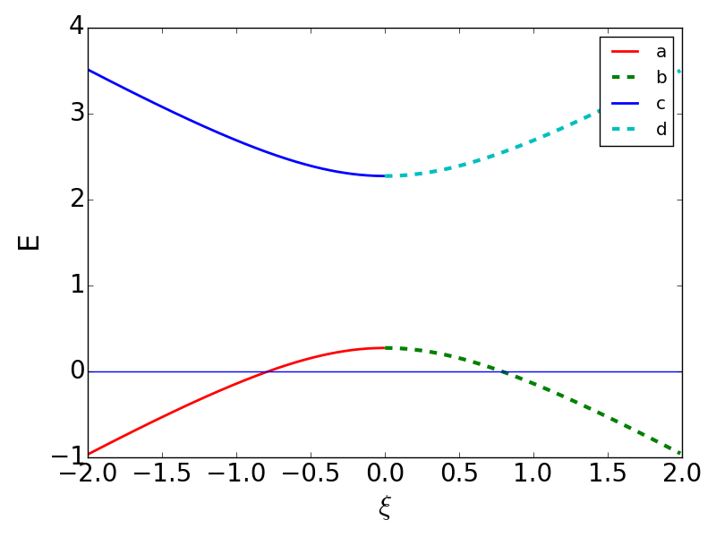
Figure 1: (color online) The four (Eq. 46) branches [solid red ($a,\xi<0$), dashed green ($b,\xi>0$), solid blue ($c,\xi<0$), and dashed cyan ($d,\xi>0$) ] for $\mu=100$, $\Delta=1$MeV, $\delta\mu=1.4$MeV, $b=1.3$MeV, and $\cos\theta=-0.1$ (Eq. 43). The gap between the lower and upper branches is $2\Delta$, and for $\Delta\ll T$ only excitations near $E=0$ participate in transport. 

III.3 Spectrum of excitations

The mean field lagrangian for $ur$, $ug$, $dr$, and $dg$ quarks  Rajagopal and Wilczek (2000) quarks is given by

$$\begin{split}{{\cal{L}}}&=-2\frac{\Delta^{*}\Delta}{\lambda}+\\ &\frac{1}{2}\Psi^{\dagger}_{4L}\left(\begin{array}[]{cc}i\bar{\sigma}^{\mu}\partial_{\mu}+\mu_{u}&-\Delta e^{2i{\bf{b}}\cdot{\bf{r}}}\\ -\Delta^{*}e^{-2i{\bf{b}}\cdot{\bf{r}}}&i\sigma^{\mu}\partial_{\mu}-\mu_{d}\end{array}\right)\Psi_{4L}+(L\rightarrow R)\;,~{}\end{split}$$ (30)

where

$$\begin{split}\Psi_{4L}(x)&=\left(\begin{array}[]{c}u_{rLa}(x)\\ u_{gLa}(x)\\ -\epsilon^{{\dot{a}}{\dot{b}}}d^{*}_{gL{\dot{b}}}(x)\\ +\epsilon^{{\dot{a}}{\dot{b}}}d^{*}_{rL{\dot{b}}}(x)\end{array}\right)\end{split}$$ (31)

or more compactly as

$$\begin{split}\Psi_{4L}(x)&=\left(\begin{array}[]{c}u_{L}(x)\\ -[\epsilon^{c}]d^{C}_{L}(x)\\ \end{array}\right)\end{split}$$ (32)

where, $[\epsilon^{c}]_{cc^{\prime}}=\epsilon_{cc^{\prime}}$ is the antisymmetric matrix in a two dimensional sub-space of color.

For the $ur$, $dg$ quarks, it can be written as

$$\begin{split}{{\cal{L}}}&=-\frac{\Delta^{*}\Delta}{\lambda}+\\ &\frac{1}{2}\Psi^{\dagger}_{L}\left(\begin{array}[]{cc}i\bar{\sigma}^{\mu}\partial_{\mu}+\mu_{u}&-\Delta e^{2i{\bf{b}}\cdot{\bf{r}}}\\ -\Delta^{*}e^{-2i{\bf{b}}\cdot{\bf{r}}}&i\sigma^{\mu}\partial_{\mu}-\mu_{d}\end{array}\right)\Psi_{L}+(L\rightarrow R)~{}\end{split}$$ (33)

where Rajagopal and Wilczek (2000),

$$\Delta=\lambda\Theta_{3}$$ (34)

and the two dimensional Nambu-Gorkov spinors $\Psi$ are defined as

$$\begin{split}\Psi_{L}(x)&=\left(\begin{array}[]{c}u_{rLa}(x)\\ -\epsilon^{{\dot{a}}{\dot{b}}}d^{*}_{gL{\dot{b}}}(x)\end{array}\right)=\left(\begin{array}[]{c}u_{rL}(x)\\ -d_{gL}^{C}(x)\end{array}\right)\\ \Psi_{L}^{\dagger}(x)&=(u_{rL{\dot{a}}}^{*}(x),-\epsilon^{ac}d_{gLc}(x))=(u_{rL}^{\dagger}(x),-d_{gL}^{C\dagger}(x))\;,\end{split}$$ (35)

where $x=(t,{\bf{r}})$.

Similarly, the Nambu-Gorkov spinor for $ug-dr$

$$\begin{split}\Xi_{L}(x)&=\left(\begin{array}[]{c}u_{gLa}(x)\\ \epsilon^{{\dot{a}}{\dot{b}}}d^{*}_{rL{\dot{b}}}(x)\end{array}\right)=\left(\begin{array}[]{c}u_{gL}(x)\\ d_{rL}^{C}(x)\end{array}\right)\\ \Xi_{L}^{\dagger}(x)&=(u_{gL{\dot{a}}}^{*}(x),\epsilon^{ac}d_{rLc}(x))=(u_{gL}^{\dagger}(x),d_{rL}^{C\dagger}(x))\;,\end{split}$$ (36)

has the same form as Eq. 33.

For $h=-1/2$, ${\bf{p}}\cdot\sigma=-p=-|{\bf{p}}|$, (This the correct helicity for $L$ handed quarks. These are the “large” components in the Fourier decomposition of the Dirac spinor Mannarelli et al. (2006).) and the dispersion relation for the paired quarks is obtained by diagonalising finding the energy eigenvalues of

$$\left(\begin{array}[]{cc}(E-|{\bf{p}}+{\bf{b}}|)+\mu_{u}&-\Delta\\ -\Delta^{*}&(E+|{\bf{p}}-{\bf{b}}|)-\mu_{d}\end{array}\right)\;.$$ (37)

The eigenvalues and the eigenvectors are given by,

$$\begin{split}E_{1}=&(|{\bf{p}}+{\bf{b}}|-|{\bf{p}}-{\bf{b}}|+2\delta\mu)/2\\ &-\sqrt{\xi^{2}+\Delta^{2}}\\ \Psi_{1}=\left(\begin{array}[]{c}\Phi_{11}\\ \Phi_{12}\end{array}\right)&=\left(\begin{array}[]{c}\frac{1}{\sqrt{2}}\sqrt{1-\frac{\xi}{\epsilon}}\\ -e^{-i\phi}\frac{1}{\sqrt{2}}\sqrt{1+\frac{\xi}{\epsilon}}\end{array}\right)~{}\end{split}$$ (38)

and,

$$\begin{split}E_{2}=&(|{\bf{p}}+{\bf{b}}|-|{\bf{p}}-{\bf{b}}|+2\delta\mu)/2\\ &+\sqrt{\xi^{2}+\Delta^{2}}\\ \Psi_{2}=\left(\begin{array}[]{c}\Phi_{21}\\ \Phi_{22}\end{array}\right)&=\left(\begin{array}[]{c}\frac{1}{\sqrt{2}}\sqrt{1+\frac{\xi}{\epsilon}}\\ e^{-i\phi}\frac{1}{\sqrt{2}}\sqrt{1-\frac{\xi}{\epsilon}}\end{array}\right)~{}\end{split}$$ (39)

$\xi=(|{\bf{p}}+{\bf{b}}|+|{\bf{p}}-{\bf{b}}|-2{\mu})/2$, $\epsilon=\sqrt{\xi^{2}+\Delta^{2}}$ and $\phi$ is the phase of $\Delta$. $\mu=(\mu_{u}+\mu_{d})/2$ is the mean of the chemical potentials and $\mu_{d}-\mu_{u}=2\delta\mu$.

The Bogoliubov coefficients can be arranged in a orthonormal matrix form,

$$\begin{split}[\Phi]=\left(\begin{array}[]{cc}\Phi_{11}&\Phi_{21}\\ \Phi_{12}&\Phi_{22}\end{array}\right)~{}\end{split}$$ (40)

We simplify the momentum integrals Eq. 21 in the limit $\mu\gg\delta\mu,\;b,\;\Delta$, and $\mu,\gg T$. Near the Fermi surface

$$\begin{split}\frac{d^{3}p}{(2\pi)^{3}}&=\frac{p^{2}dpd\Omega}{(2\pi)^{3}}\approx\mu^{2}d\xi\frac{d\Omega}{(2\pi)^{3}}~{}\;.\end{split}$$ (41)

In this approximation

$$\begin{split}E_{1}({\bf{p}})&=\delta\mu+{\bf{b}}\cdot{\bf{v}}_{F}-\sqrt{\xi^{2}+\Delta^{2}}\\ E_{2}({\bf{p}})&=\delta\mu+{\bf{b}}\cdot{\bf{v}}_{F}+\sqrt{\xi^{2}+\Delta^{2}}~{}\;,\end{split}$$ (42)

or in polar coordinates with $\hat{b}=\hat{z}$,

$$\begin{split}E_{1}(\xi,\theta)&=\delta\mu+b\cos\theta-\sqrt{\xi^{2}+\Delta^{2}}\\ E_{2}(\xi,\theta)&=\delta\mu+b\cos\theta+\sqrt{\xi^{2}+\Delta^{2}}~{}\;,\end{split}$$ (43)

where $\xi=p-\mu$ and ${\bf{v}}_{F}=(d\xi/dp)\hat{p}=\hat{p}$ is the Fermi velocity.

The mode decomposition of $\Psi$ is

$$\begin{split}\Psi_{L}(x)&=\int\frac{d^{4}p}{(2\pi)^{4}}e^{-ip_{\mu}x^{\mu}}[\\ &\phantom{+}(2\pi)\delta(p^{0}-E_{1})\left(\begin{array}[]{c}\Phi_{11}e^{i{\bf{b}}\cdot{\bf{r}}}\xi_{-}(p)\\ \Phi_{12}e^{-i{\bf{b}}\cdot{\bf{r}}}\xi_{-}(p)\end{array}\right)\gamma_{L}\\ &+(2\pi)\delta(p^{0}-E_{2})\left(\begin{array}[]{c}\Phi_{21}e^{i{\bf{b}}\cdot{\bf{r}}}\xi_{-}(p)\\ \Phi_{22}e^{-i{\bf{b}}\cdot{\bf{r}}}\xi_{-}(p)\end{array}\right)\chi_{L}]~{}\;,\end{split}$$ (44)

where $\xi(-)$ is the two component spinor satisfying

$${\bf{p}}\cdot\sigma\xi_{-}(p)=-p\xi_{-}(p)\;.$$ (45)

Now, with the two energy eigenstates Eq. 42 in hand, it is tempting to treat Eq. 21 as a two species problem in the eigenstates Eq. 38 and Eq. 39 which corresponds to an appropriate linear combination of $u$ particles and $d$ holes (Eq. 44).

Since, $u$ and $d$ quarks have different couplings (which is the case for $\tilde{Q}$ “photons”) with the gauge fields, we treat it as a four species problem, labelling the species as

$$\begin{split}a&\rightarrow E_{1},\;\xi<0\\ b&\rightarrow E_{1},\;\xi>0\\ c&\rightarrow E_{2},\;\xi<0\\ d&\rightarrow E_{2},\;\xi>0~{}\;.\end{split}$$ (46)

This labelling also clarifies the contributions to the shear viscosity from the various branches of the Bogoliubov dispersions (Fig.(1)).

The matrix equation, Eq. 21, is now a $4\times 4$ matrix equation which gives the four relaxation times $\tau_{i}$ and the viscosities can be found by using Eq. 28.

III.4 Interactions

The interactions between the quarks are mediated by the gauge bosons: the gluons and the photon. The gluon-quark vertex is

$$S_{g}=(g)\int d^{4}x\bar{\psi}\gamma^{\mu}t^{m}\psi A_{\mu}^{m}$$ (47)

where $g$ is the strong coupling constant, and the photon-quark vertex is

$$S_{e}=(-e)\int d^{4}x\bar{\psi}\gamma^{\mu}Q\psi A_{\mu}$$ (48)

where $t^{m}$ are the Gell-Mann matrices and $Q={\rm{diag}}\{2/3,-1/3\}$ in flavor space.

To contrast with the properties of the mediators in the FF phase, we revise the main features in the unpaired phase. Transport in the unpaired phase is dominated by the quarks and the electron. The mediators of their interactions have the following properties.

The longitudinal components of the gluons as well as the photon are Debye screened. The relevant propagators for the gauge boson are

$$\begin{split}\frac{i}{-{\bf{q}}^{2}-\Pi_{l}(q)}[\hat{q}_{i}\hat{q}_{j}]\delta^{ab}~{}\end{split}$$ (49)

where $(\omega,{\bf{q}})=p_{3}^{\mu}-p_{1}^{\mu}=p_{2}^{\mu}-p_{4}^{\mu}$ is the four momentum carried by the gauge field, ${\bf{q}}^{2}={\bf{q}}_{i}{\bf{q}}_{i}$, $q=|{\bf{q}}|$, and $\Pi_{l}$  is longitudinal polarization tensor. We have neglected $\omega^{2}$ in the propagator. In the limit of small ${\bf{q}}$,

$$\begin{split}\Pi_{l}(q)\approx\Pi_{l}(0)=m_{D}^{2}=2N_{f}(\frac{g}{2})^{2}\frac{\mu^{2}}{\pi^{2}}~{}\;,\end{split}$$ (50)

up to corrections of the order $(\delta\mu/\mu)^{2}$. $N_{f}=2$ in the two-flavor FF problem.

In the absence of pairing the transverse gluons are dynamically screened

$$\begin{split}\frac{i}{\omega^{2}-{\bf{q}}^{2}-\Pi_{t}(q)}[\delta_{ij}-\hat{q}_{i}\hat{q}_{j}]\delta^{ab}~{}\end{split}$$ (51)

where $\Pi_{t}$ is transverse polarization function, which in the limit of small $\omega,q$,

$$\begin{split}\Pi_{t}(\omega,q)\approx(\frac{-i\pi\omega}{4q})2N_{f}(\frac{g}{2})^{2}\frac{\mu^{2}}{\pi^{2}}~{}\;.\end{split}$$ (52)

Since the energy exchange, $\omega$, is governed by the temperature, while the momentum exchange can be much larger (typically of the order of $g\mu$), the transverse gluons have a longer range compared to the longitudinal and therefore their exchange is the dominant scattering mechanism for the quarks. Consequently, the momentum exchange $q$ that dominates the collision integral for the transverse gauge bosons is $\sim(T\Pi_{l}(0))^{1/3}$ Baym et al. (1990), while for the longitudinal gauge bosons it is $\sim(\Pi_{l}(0))^{1/2}$.

Similarly, for the photon the Debye screening mass can be obtained from Eq. 50 by replacing $2N_{f}(\frac{g}{2})^{2}$ by $N_{c}e^{2}(Q_{u}^{2}+Q_{d}^{2})$ and the transverse polarization $\Pi_{t}$ can be obtained from Eq. 52 by replacing $2N_{f}(\frac{g}{2})^{2}$ by $N_{c}e^{2}(Q_{u}^{2}+Q_{d}^{2})$ with $N_{c}=3$.

We now consider the gauge bosons in the two-flavor FF phase. As far as the Debye screening masses are concerned, these are determined by the total density of gapless states. For gluons that couple with the species that participate in pairing, this density of states is affected by two competing effects.

First, there is a geometric factor associated with a reduction in size of the surface of gapless excitations Alford et al. (2001b) (Appendix A),

$$\begin{split}\frac{\mu^{2}}{\pi^{2}}\rightarrow\frac{\mu^{2}}{\pi^{2}}(1-2\frac{\Delta}{b}),\end{split}$$ (53)

since the blocking region is absent for $\cos\theta\in[\frac{\delta\mu-\Delta}{b},\frac{\delta\mu+\Delta}{b}]$.

Second, the Fermi velocity on the surface of gapless excitations is reduced due to pairing. In spherical coordinates, the Fermi velocity is given by

$$\begin{split}\frac{dE}{d{\bf{p}}}(\xi,\theta)&=\hat{p}\frac{\xi}{\sqrt{\xi^{2}+\Delta^{2}}}|_{\xi=\sqrt{(\delta\mu+b\cos\theta)^{2}-\Delta^{2}}}+\frac{b}{p}\hat{\theta}\\ &\approx\hat{p}\frac{\xi}{\sqrt{\xi^{2}+\Delta^{2}}}|_{\xi=\sqrt{(\delta\mu+b\cos\theta)^{2}-\Delta^{2}}}<\hat{p}\;.\end{split}$$ (54)

The reduction of the velocity enhances the density of states at the gapless point Alford et al. (2005b) for certain values of $\theta$.

Consequently, we expect that for the gluons

$$\begin{split}\Pi_{l}(0)=2N_{f}(\frac{g}{2})^{2}\frac{\mu^{2}}{\pi^{2}}f(\frac{\Delta}{\delta\mu},\frac{b}{\delta\mu})~{}\end{split}$$ (55)

where $f$ is expected to be of order $1$ Casalbuoni et al. (2002). Similar arguments hold for the photon.

We leave a detailed analysis of screening of the longitudinal modes for future work. The two main points we want to emphasize are as follows. First the longitudinal $t^{1},t^{2},t^{3}$ gluons are screened and hence unlike in the $2{\rm{SC}}$ phase Rischke et al. (2001) the $ur-dg-ug-dr$ quarks are not confined. Second, the longitudinal modes of all the mediators are screened and therefore can be ignored compared to the Landau damped transverse mediators while calculating the transport properties. The transverse screening masses for the gauge bosons in the two-flavor FF phase were analyzed in detail in Ref. Giannakis and Ren (2005a, b) and we summarize the main conclusions here.

In contrast with unpaired phase, in the two-flavor FF phase, the Meissner masses for the $t^{4}\dots t^{7}$ gluons are non-zero Giannakis and Ren (2005a, b); Ciminale et al. (2006). The FF condensate cures the instability seen in the gapless $2{\rm{SC}}$ phase, and the squares of all the four Meissner masses are positive, and are functions of $\Delta,\delta\mu,\mu$, and $b$.

The Meissner masses tend to $0$ as $\Delta\rightarrow 0$ and hence naturally

$$m_{M}^{2}\sim(\frac{g}{2})^{2}\frac{\mu^{2}}{\pi^{2}}\frac{\Delta^{2}}{\delta\mu^{2}}\;.$$ (56)

$\Delta^{2}$ tends to $0$ at $\delta\mu=0.754\Delta_{2{\rm{SC}}0}$, i.e., the transition point. Away from the transition point, $\Delta$ is much larger than $T$, and screening is strong if the Meissner mass is non-zero.

The fate of the $t^{8}$ and the photon is more interesting. As in the $2{\rm{SC}}$ phase, the condensate is neutral under the linear combination associated with the $\tilde{Q}$ charge which is unscreened. The $\tilde{Q}$ photon is weakly coupled to the quarks and is less important than the unscreened gluons Rajagopal and Wilczek (2000). The orthogonal linear combination,

$$\begin{split}A_{\mu}^{X}=\cos\varphi A_{\mu}^{8}+\sin\varphi A_{\mu}^{Q}\;,\end{split}$$ (57)

with

$$\begin{split}\cos\varphi=\frac{\sqrt{3}g}{\sqrt{e^{2}+3g^{2}}}\;,\end{split}$$ (58)

is strongly coupled.

Because ${\bf{b}}$ chooses a particular direction, the transverse polarization tensor is not invariant in the range of the transverse projection operator

$$[\delta_{ij}-\hat{q}_{i}\hat{q}_{j}]~{}\;.$$ (59)

Ref. Giannakis and Ren (2005b) showed that a further projection by $b^{i}b^{j}$ (note that Ref. Giannakis and Ren (2005b) uses $q$ to denote what we call ${\bf{b}}$ and $k$ to denote what we call $q$) gives a polarization tensor which vanishes in the $0$ momentum limit (the “longitudinal transverse gluon”). The projection on to $\delta^{ij}-b^{i}b^{j}$ (the “transverse transverse gluon”) has a finite Meissner mass.

While the “longitudinal transverse” part of $A_{\mu}^{X}$ is long ranged as well as strongly coupled, its contribution is smaller compared to the $t^{1}$, $t^{2}$, $t^{3}$ gluons as we argue below (below Eq. 75). The transverse $t^{1},t^{2},t^{3}$ gluons are massless as in the $2{\rm{SC}}$ phase Casalbuoni et al. (2002); Giannakis and Ren (2005b). What has not been appreciated in the literature is that they are Landau damped.

To express the transverse polarization tensor in a compact form we choose an orthogonal basis for the range of Eq. 59 as follows.

$$\begin{split}\hat{y}^{\prime}&=\frac{\hat{b}\times\hat{q}}{|\hat{b}\times\hat{q}|}\\ \hat{x}^{\prime}&=\hat{y}^{\prime}\times\hat{b}~{}\;.\end{split}$$ (60)

On general grounds,

$$\begin{split}\Pi^{i^{\prime}j^{\prime}}_{t}(\omega,{\bf{q}})=(\frac{-i\pi\omega}{4q})\Bigl{[}2N_{f}(\frac{g}{2})^{2}\frac{\mu^{2}}{\pi^{2}}\Bigr{]}h^{i^{\prime}j^{\prime}}_{t}(\frac{\Delta}{\delta\mu},\frac{b}{\delta\mu},\cos\theta_{bq})~{}\;.\end{split}$$ (61)

For unpaired quark matter $h^{i^{\prime}j^{\prime}}=\delta^{i^{\prime}j^{\prime}}$.

Numerical results for the Landau damping coefficient for $b/\delta\mu=\zeta$ are well described by the expressions

$$\begin{split}h^{x^{\prime}x^{\prime}}_{t}(\frac{\Delta}{\delta\mu},\frac{b}{\delta\mu},\cos\theta_{bq})&\approx 1-(\frac{\Delta}{b})^{1/4}\frac{1}{1.65}(1-\cos\theta_{bq}^{4})^{1/2}\\ h^{y^{\prime}y^{\prime}}_{t}(\frac{\Delta}{\delta\mu},\frac{b}{\delta\mu},\cos\theta_{bq})&\approx 1-(\frac{\Delta}{b})\frac{1}{1.75}(1-\cos\theta_{bq}^{2})^{1/2}\\ h^{x^{\prime}y^{\prime}}_{t}(\frac{\Delta}{\delta\mu},\frac{b}{\delta\mu},\cos\theta_{bq})&\approx 0\;.~{}\end{split}$$ (62)

We note that $h<1$, which is expected because the gapless surface (For a quick refresher on the gapless modes in the FF phase see Appendix A. For details see Alford et al. (2001b); Bowers and Rajagopal (2002); Bowers (2003); Mannarelli et al. (2006)) in the FF phase has a smaller surface area compared to the unpaired phase The details of the calculation will be given elsewhere InP .

To summarize, scattering between the $ur-dg-ug-dr$ quarks is dominated by exchange of the transverse $t^{1},t^{2},t^{3}$ gluons. Their propagator is of the form

$$\begin{split}iD_{\mu\nu}^{ab}&=\frac{i}{\omega^{2}-q^{2}-\Pi_{t}^{i^{\prime}j^{\prime}}(\omega,{\bf{q}})}[{\cal{P}}_{\mu\nu}^{i^{\prime}j^{\prime}}]\delta^{ab}~{}\;.\end{split}$$ (63)

The projection operator,

$${\cal{P}}_{\mu\nu}^{i^{\prime}j^{\prime}}=\delta_{\mu}^{i^{\prime}}\delta_{\nu}^{j^{\prime}}$$ (64)

projects into the subspace spanned by the unit vectors $e_{i}^{\prime},e_{j}^{\prime}$ (Eq. 60), $\Pi_{t}^{i^{\prime}j^{\prime}}(\omega,{\bf{q}})$ are given by Eq. 61.

The interaction can be written in terms of the Nambu-Gorkov spinors  as follows.

$$\begin{split}S_{g}&=(g)\int d^{4}x\bar{\psi}\gamma^{\mu}t^{m}\psi A_{\mu}^{m}\\ &=(g)\int d^{4}x\bar{\psi}_{L}\bar{\sigma}^{\mu}t^{m}\psi_{L}A_{\mu}^{m}+(g)\int d^{4}x\bar{\psi}_{R}{\sigma}^{\mu}t^{m}\psi_{R}A_{\mu}^{m}\;.\end{split}$$ (65)

Going to momentum bases and using Eq. 44 we obtain,

$$\begin{split}&{\cal{L}}_{AL}=\int\frac{d^{4}p_{1}}{(2\pi)^{4}}\frac{d^{4}p_{3}}{(2\pi)^{4}}\\ &{g}\left((\Phi^{*}_{11}\;\Phi^{*}_{12})\gamma_{L}^{\dagger}(2\pi)\delta(p_{3}^{0}-E_{1})+(\Phi^{*}_{21}\;\Phi^{*}_{22})\chi_{L}^{\dagger}(2\pi)\delta(p_{3}^{0}-E_{2})\right)\\ &\left(\begin{array}[]{cc}1\xi_{-}^{\dagger}(p_{3}){\bar{\sigma}}^{\mu}\xi_{-}(p_{1})t^{m}&0\\ 0&-1\xi_{-}^{\dagger}(p_{3})C{\bar{\sigma}}^{T\mu}C^{\dagger}\xi_{-}(p_{1})\epsilon_{c}^{\dagger}(t^{m})^{T}\epsilon_{c}\\ \end{array}\right)\\ &\left((\begin{array}[]{c}\Phi_{11}\\ \Phi_{12}\end{array})\gamma_{L}(2\pi)\delta(p_{1}^{0}-E_{1})+(\begin{array}[]{c}\Phi_{21}\\ \Phi_{22}\end{array})\chi_{L}(2\pi)\delta(p_{1}^{0}-E_{2})\right)\\ &A^{a}_{\mu}(p_{3}-p_{1})\;.\end{split}$$ (66)

Now we can use the conjugation relation for $t^{1},\;t^{2},\;t^{3}$ generators,

$$\begin{split}-1\epsilon_{c}^{\dagger}(t^{m})^{T}\epsilon_{c}&=t^{m}\;,\end{split}$$ (67)

and the $t^{m}$ get decoupled from the Nambu-Gorkov structure. [This step won’t work for the other ${\rm{SU}}(3)$ generators and works because the ${\rm{SU}}(2)$ subgroup generated by $t^{1}\dots t^{3}$ is unbroken in two-flavor FF. See Eq. 99 for an analysis of a broken generator.] We also use the conjugation relation for ${\bar{\sigma}}^{\mu}$,

$$\begin{split}C{\bar{\sigma}}^{T\mu}C^{\dagger}=\sigma^{\mu}\;,\end{split}$$ (68)

to simplify the spin structure. This gives,

$$\begin{split}&{\cal{L}}_{AL}=\int\frac{d^{4}p_{1}}{(2\pi)^{4}}\frac{d^{4}p_{3}}{(2\pi)^{4}}{g}\\ &\left((\Phi^{*}_{11}\;\Phi^{*}_{12})\gamma_{L}^{\dagger}(2\pi)\delta(p_{3}^{0}-E_{1})+(\Phi^{*}_{21}\;\Phi^{*}_{22})\chi_{L}^{\dagger}(2\pi)\delta(p_{3}^{0}-E_{2})\right)\\ &\left(\begin{array}[]{cc}1\xi_{-}^{\dagger}(p_{3}){\bar{\sigma}}^{\mu}\xi_{-}(p_{1})&0\\ 0&1\xi_{-}^{\dagger}(p_{3})\sigma^{\mu}\xi_{-}(p_{1})\\ \end{array}\right)\\ &\left((\begin{array}[]{c}\Phi_{11}\\ \Phi_{12}\end{array})\gamma_{L}(2\pi)\delta(p_{1}^{0}-E_{1})+(\begin{array}[]{c}\Phi_{21}\\ \Phi_{22}\end{array})\chi_{L}(2\pi)\delta(p_{1}^{0}-E_{2})\right)\\ &t^{m}A^{m}_{\mu}(p_{3}-p_{1})~{}\;.\end{split}$$ (69)

Similarly, for $R$ we obtain

$$\begin{split}&{\cal{L}}_{AR}=\int\frac{d^{4}p_{1}}{(2\pi)^{4}}\frac{d^{4}p_{3}}{(2\pi)^{4}}{g}\\ &\left((\Phi^{*}_{11}\;\Phi^{*}_{12})\gamma_{R}^{\dagger}(2\pi)\delta(p_{3}^{0}-E_{1})+(\Phi^{*}_{21}\;\Phi^{*}_{22})\chi_{R}^{\dagger}(2\pi)\delta(p_{3}^{0}-E_{2})\right)\\ &\left(\begin{array}[]{cc}1\xi_{+}^{\dagger}(p)\sigma^{\mu}\xi_{+}(p)&0\\ 0&1\xi_{+}^{\dagger}(p){\bar{\sigma}}^{\mu}\xi_{+}(p)\\ \end{array}\right)\\ &\left((\begin{array}[]{c}\Phi_{11}\\ \Phi_{12}\end{array})\gamma_{R}(2\pi)\delta(p_{1}^{0}-E_{1})+(\begin{array}[]{c}\Phi_{21}\\ \Phi_{22}\end{array})\chi_{R}(2\pi)\delta(p_{1}^{0}-E_{2})\right)\\ &t^{m}A^{m}_{\mu}(p_{3}-p_{1})~{}\;.\end{split}$$ (70)

A nice way to separate the spinor and the Nambu-Gorkov structure is to re-combine the $L$ (69) and $R$ (69) components

$$\begin{split}&{\cal{L}}_{ALR}=\int\frac{d^{4}p_{1}}{(2\pi)^{4}}\frac{d^{4}p_{3}}{(2\pi)^{4}}\\ &{g}\left(\bar{u}_{s}(p_{3})\gamma^{\mu}u_{s}(p_{1})\right)\\ &\left((\Phi^{*}_{11}\;\Phi^{*}_{12})\gamma_{s}^{\dagger}(2\pi)\delta(p_{3}^{0}-E_{1})+(\Phi^{*}_{21}\;\Phi^{*}_{22})\chi_{s}^{\dagger}(2\pi)\delta(p_{3}^{0}-E_{2})\right)\\ &\left((\begin{array}[]{c}\Phi_{11}\\ \Phi_{12}\end{array})\gamma_{s}(2\pi)\delta(p_{1}^{0}-E_{1})+(\begin{array}[]{c}\Phi_{21}\\ \Phi_{22}\end{array})\chi_{s}(2\pi)\delta(p_{1}^{0}-E_{2})\right)\\ &t^{m}A_{\mu}^{m}(p_{3}-p_{1})~{}\;.\end{split}$$ (71)

The final ingredient we need is the simplification of the color structure in the interaction. For this we use the relation ($a=1,2,3$)

$$\begin{split}t^{m}_{ij}t^{m}_{kl}=[\frac{-1}{4}\delta_{ij}\delta_{kl}+\frac{1}{2}\delta_{il}\delta_{kj}]\end{split}$$ (72)

Summing over the final colors ($j,l$) and averaging over the initial colors ($i,k$) gives (the sum over colors runs over only two colors $r$ and $g$)

$$\begin{split}\frac{1}{4}t^{m}_{ij}t^{m}_{kl}t^{n*}_{ij}t^{n*}_{kl}&=\frac{1}{4}t^{m}_{ij}t^{m}_{kl}t^{n}_{ji}t^{n}_{lk}\\ &=\frac{3}{16}\;.\end{split}$$ (73)

Therefore, the square of the scattering matrix element averaged over initial color and spin and summed over the final color and spin are given by 

$$\begin{split}|i\bar{\cal{M}}|^{2}&=3(\frac{g}{2})^{4}\\ &|(\Phi^{*}_{i_{3}1}\;\Phi^{*}_{i_{3}2})\left(\begin{array}[]{c}\Phi_{i_{1}1}\\ \Phi_{i_{1}2}\end{array}\right)|^{2}|(\Phi^{*}_{i_{4}1}\;\Phi^{*}_{i_{4}2})\left(\begin{array}[]{c}\Phi_{i_{2}1}\\ \Phi_{i_{2}2}\end{array}\right)|^{2}\\ &\frac{1}{4}\frac{1}{2p_{1}2p_{2}2p_{3}2p_{4}}{\rm{tr}}[p\!\!\!/_{3}\gamma^{\mu}p\!\!\!/_{1}\gamma^{\nu}]{\rm{tr}}[p\!\!\!/_{4}\gamma^{\sigma}p\!\!\!/_{2}\gamma^{\lambda}]{D}_{\mu\sigma}{D}_{\nu\lambda}\\ &=3(\frac{g}{2})^{4}\delta_{i_{1}i_{3}}\delta_{i_{2}i_{4}}\\ &\frac{1}{4}\frac{1}{2p_{1}2p_{2}2p_{3}2p_{4}}{\rm{tr}}[p\!\!\!/_{3}\gamma^{\mu}p\!\!\!/_{1}\gamma^{\nu}]{\rm{tr}}[p\!\!\!/_{4}\gamma^{\sigma}p\!\!\!/_{2}\gamma^{\lambda}]{D}_{\mu\sigma}{D}_{\nu\lambda}~{}\;,\end{split}$$ (75)

where $i_{1},\;i_{2},\;i_{3},\;$ and $i_{4}$ run over $1,\;2$ where $1$ corresponds to $\gamma$ and $2$ to $\xi$. Note that the orthogonality of $[\Phi]$ (Eq. 40) ensures that $i_{1}=i_{3}$ and $i_{2}=i_{4}$, and the nature of the Bologliubov particles doesn’t change at the vertex. This can be traced to the residual ${\rm{SU}}(2)$ symmetry. The factor ${1}/{(2p_{1}2p_{2}2p_{3}2p_{4})}$ appears in $|{\cal{M}}|^{2}$ due to the convention of the phase space integrals in Eq. 21: the spinors $u_{s}$ are normalized to be dimensionless.

Eq. 75 can also be used to complete the argument that we made earlier about why the exchange of transverse $A^{X}$ is less important than the exchange of $t^{1}$, $t^{2}$, $t^{3}$ even though they have $0$ Meissner mass. In matrix elements the exchange of $A^{X}$ comes with a coherence factor (Eq. 99) where two terms of similar size cancel. This is because $\Phi_{i_{3}1},\;\Phi_{i_{3}1},\;\Phi_{i_{1}2}^{*}$, and $\Phi_{i_{1}2}$ in Eq. 99 are all roughly $1/\sqrt{2}$ for $\xi\approx 0$ and in Eq. 99 their products appear with a $-$ sign. On the other hand the coherence factors in Eq. 75 add for $t^{1},t^{2},t^{3}$ gluons. Therefore we expect the numerical contribution from $A_{\mu}^{X}$ to be smaller than the contribution from $t^{1},t^{2},t^{3}$ gluons. (There is an additional reduction by a factor of $\sim 1/2$ because the “transverse transverse gluon” is massive.) Therefore we neglect the scatterings mediated by $A_{\mu}^{X}$. This numerical suppression is not parametric and in a future, more complete calculation, these scatterings should be included. We note that $A_{\mu}^{X}$ induces coupling between the $b$ quarks and the paired quarks and complicates the Boltzmann equation Eq. 21 significantly.

There are additional mediators of quark-quark interactions in the two-flavor FF phase. Phonons Casalbuoni et al. (2001b) associated with the periodicity of the condensate Mannarelli et al. (2007); Radzihovsky and Vishwanath (2009), are derivatively coupled to the fermion fields.

The interaction between quark species $i$ and $j$, and phonon $\varphi^{a}$ can generically be written as

$$\begin{split}{\cal{L}}_{\varphi\psi}=\frac{c_{\mu}}{f_{\varphi}^{ij}}\partial_{\mu}\varphi^{a}\bar{\psi}_{j}\gamma^{\mu}\psi_{i}~{}\;.\end{split}$$ (76)

where $c_{\mu}$ is naturally of the order of $v_{F}$.

Therefore, the scattering matrix in the absence of pairing can be written as

$$\begin{split}i{\cal{M}}\sim(\frac{c_{\mu}q_{\mu}c_{\nu}q_{\nu}}{(f_{\varphi}^{ij})^{2}})\frac{i}{\omega^{2}-v_{\varphi}^{2}q^{2}}[\bar{u}_{3}\gamma^{\mu}u_{1}][\bar{u}_{4}\gamma^{\mu}u_{2}]\end{split}$$ (77)

where $q_{\mu}=(\omega,{\bf{q}})_{\mu}$ is the four momentum carried by the phonon. For $\omega\ll q$

$$\begin{split}i{\cal{M}}\sim(\frac{c_{i}^{2}}{(f_{\varphi}^{ij})^{2}})\frac{i}{-v_{\varphi}^{2}}[\bar{u}_{3}\gamma^{0}u_{1}][\bar{u}_{4}\gamma^{0}u_{2}]~{}\;.\end{split}$$ (78)

This should be compared with the matrix element for the exchange of a Debye screened gauge field.

$$\begin{split}i{\cal{M}}\sim(ig)^{2}\frac{i}{q^{2}+m_{D}^{2}}[\bar{u}_{3}\gamma^{0}u_{1}][\bar{u}_{4}\gamma^{0}u_{2}]\\ \sim-i(g)^{2}\frac{1}{m_{D}^{2}}[\bar{u}_{3}\gamma^{0}u_{1}][\bar{u}_{4}\gamma^{0}u_{2}]~{}\;.\end{split}$$ (79)

Noting that both $m_{D}$ and $f_{\varphi}$ can be related to thermodynamic susceptibilities Son and Stephanov (2000a), and that $v_{\varphi}\sim 1$ in relativistic systems

$$\begin{split}m_{D}^{2}\sim g^{2}f_{\varphi}^{2}\end{split}$$ (80)

we see that Eq. 78 is of the same order as Eq. 79 . Therefore, the contributions to quark-quark scattering from phonon exchanges can be ignored in our calculation.

III.5 Contribution of phonons

Phonons, the Goldstone modes associated with broken symmetries, are also low energy modes. Here we make a quick estimate of their contribution to transport and to the collision integral. They are not relevant in the FF phase but play an important role in gapped phases.

III.5.1 Quark-Phonon scattering

For quark-phonon scattering, the collision term is

$$\begin{split}[\Gamma_{i}(p_{i})]&=-\sum_{3}\int\;\frac{d^{3}l}{(2\pi)^{3}}\frac{d^{3}p_{3}}{(2\pi)^{3}}(2\pi)^{4}\\ &[{\hat{f}}_{i}{\hat{b}}_{2}(1-{\hat{f}}_{3})\delta^{(4)}(p_{i}+l-p_{3})|{\cal{M}}(il\rightarrow 3)|^{2}\\ &+{\hat{f}}_{i}(1+{\hat{b}}_{2})(1-{\hat{f}}_{3})\delta^{(4)}(p_{i}-l-p_{3})|{\cal{M}}(i\rightarrow 3l)|^{2}\\ &-{\hat{f}}_{3}{\hat{b}}_{2}(1-{\hat{f}}_{i})\delta^{(4)}(p_{i}-l-p_{3})|{\cal{M}}(i\rightarrow 3l)|^{2}\\ &-{\hat{f}}_{3}(1+{\hat{b}}_{2})(1-{\hat{f}}_{i})\delta^{(4)}(p_{i}+l-p_{3})|{\cal{M}}(il\rightarrow 3)|^{2}]\;,\end{split}$$ (81)

where ${\hat{f}}$ and ${\hat{b}}$ are non-equilibrium distribution functions, and $l^{\mu}=(\omega,{\bf{l}})$ is the four momentum of the phonon satisfying $(\omega)^{2}-v_{\varphi}^{2}({\bf{l}}^{2})=0$.

To the lowest order in gradient of the fluid velocity $u_{a}$, ${\hat{f}}_{i}-f_{i}=\delta f_{i}=-\frac{df^{i}}{d\epsilon}[\Phi^{i}]$, where

$$\begin{split}\Phi^{i}=\sum_{(n)}\Phi^{(n)}_{i}=\sum_{(n)}3\tau^{(n)}_{i}\psi^{(n)iab}\frac{1}{2}(\partial_{a}u_{b}+\partial_{b}u_{a})\end{split}$$ (82)

Substituting Eq. 82 in the Boltzmann equation one can obtain the analogue of Eq. 21

$$\begin{split}&[R^{(n)}_{i}]=-\frac{1}{\gamma^{(n)}}\frac{1}{T}\nu_{2}\int\;\frac{d^{3}p_{i}}{(2\pi)^{3}}\frac{d^{3}l}{(2\pi)^{3}}\frac{d^{3}p_{3}}{(2\pi)^{3}}(2\pi)^{4}3\phi_{i}\cdot\\ &[f_{i}b_{2}(1-f_{3})\delta^{(4)}(p_{i}+l-p_{3})(\tau_{i}\psi_{i}^{(n)})|{\cal{M}}(il\rightarrow 3)|^{2}\\ &+f_{i}(1+b_{2})(1-f_{3})\delta^{(4)}(p_{i}-l-p_{3})(\tau_{i}\psi_{i}^{(n)})|{\cal{M}}(i\rightarrow 3l)|^{2}\\ &-f_{3}b_{2}(1-f_{i})\delta^{(4)}(p_{i}-l-p_{3})(\tau_{3}\psi_{3}^{(n)})|{\cal{M}}(i\rightarrow 3l)|^{2}\\ &-f_{3}(1+b_{2})(1-f_{i})\delta^{(4)}(p_{i}+l-p_{3})(\tau_{3}\psi_{3}^{(n)})|{\cal{M}}(il\rightarrow 3)|^{2}]\;.\end{split}$$ (83)

where $b$ is the Bose distribution.

The scattering matrix element associated with the vertex Eq. 76 is given by

$$\begin{split}|{\cal{M}}|^{2}&=|\frac{i}{f^{ij}_{\varphi}}\frac{1}{\sqrt{2\omega}\sqrt{2p_{1}}\sqrt{2p_{3}}}|^{2}4[2p_{i}\cdot lp_{3}\cdot l-p_{i}\cdot p_{3}l^{2}]|\\ &\sim\frac{l^{2}}{(f^{ij}_{\varphi})^{2}\omega}\sim\frac{\omega}{(f^{ij}_{\varphi})^{2}}\end{split}$$ (84)

where we have taken $c_{\mu}$ to be $1$ for convenience.

Simplifying the momentum integrals for the fermions ($d^{3}p_{i}$ and $d^{3}p_{3}$) as in Eq. 41, noting that $\xi_{1}$, $\xi_{3}$ and $\omega$ are all of the order of $T$, and that $\phi$ and $\psi$ are of the order of $\mu$, we can see without evaluating the integrals that,

$$\begin{split}[R_{(q-{\rm{ph}})ij}]&\sim\frac{\mu^{3}T^{4}}{(f_{\varphi}^{ij})^{2}}\sim\mu T^{4},~{}\end{split}$$ (85)

where we have used a rough estimate for $f_{\varphi}$: $f_{\varphi}\sim\mu$.

When unpaired quarks participate in transport and $T$ is much less than the chemical potential $\mu$, the contribution from Eq. 85 is subleading compared to the collision term associated with quark-quark scattering in Eq. 96. This is simple to understand because the phase space for fermions near the Fermi surface is enhanced. We shall see in Sec. IV.2.1 that this is not true for paired systems.

III.5.2 Momentum transport via phonons

If phonons are present in the low energy theory then they can also transport energy and momentum. While this is not the main topic of the paper, we make a quick estimate to see how this contribution compares with the fermionic contribution.

The kinetic theory estimate for the shear viscosity of the phonon gas is,

$$\begin{split}\eta\sim\langle n\rangle\langle p\rangle v_{\varphi}\tau_{\varphi}\;.\end{split}$$ (86)

The density of phonons at temperature $T$ is given by $\langle n\rangle\sim\frac{T^{3}}{v_{\varphi}^{3}}$ and $\langle p\rangle\sim\frac{T}{v_{\varphi}}$. Consequently,

$$\begin{split}\eta\sim\frac{1}{v_{\varphi}^{3}}T^{4}\tau_{\varphi}\;.\end{split}$$ (87)

$\tau_{\varphi}$ is very sensitive to the nature of the excitations present in the low energy theory. For example, if all the fermionic modes are gapped, then the phonons only scatter with each other. Since the phonons are coupled derivatively, the relaxation time in these cases is very long due to the small density of phonons at low temperatures, and hence the viscosity is very large. It is well known that in the absence of gapless fermions these “phonons” dominate the viscosity at low $T$ (Ref. Landau and Khalatnikov (1949); Maris (1973))

For example, if the dominant scattering rate is $2\rightarrow 2$ scattering  Rupak and Schäfer (2007); Manuel and Tolos (2011)

$$\begin{split}\eta\sim\frac{1}{v_{\varphi}^{3}}\frac{f_{\varphi}^{8}}{T^{5}}\;.\end{split}$$ (88)

In both the unpaired phase and in the FF phase, phonons can scatter off gapless fermionic excitations which have a large density of states near the Fermi surface. This effect is simply the Landau damping of the phonons. The scattering rate of the phonons is $\Gamma\sim 1/\tau\sim\frac{\mu^{2}}{f_{\varphi}^{2}}T$ Aguilera et al. (2009). A quick estimate gives

$$\begin{split}\eta\sim\frac{1}{v_{\varphi}^{3}}\frac{f_{\varphi}^{2}}{\mu^{2}}T^{3}~{}\;.\end{split}$$ (89)

In the next section we will compare the phonon contribution Eq.89 with the fermion contribution.

IV Results for a simple interaction for isotropic pairing

As discussed in the previous section, pairing affects transport properties of fermions in two important ways. First, it modifies the dispersion relations of the fermions. Second, it changes the mediator interactions.

To get some understanding of how the modification of the dispersion relations due to pairing affects transport (which is the dominant effect because of the exponential thermal factors in Eq. 21), we solve the Boltzmann equations with and without pairing for a simple system featuring two species of quarks $1$ and $2$ interacting via a single abelian gauge field $A_{\mu}$ which couples to the two species in the following manner

$$\begin{split}{\cal{L}}_{A\psi}=\frac{g}{2}\bar{\psi}A_{\mu}\gamma^{\mu}\psi~{}\;,\end{split}$$ (90)

where

$$\begin{split}\psi=(\psi_{1},\psi_{2})^{T}\;.\end{split}$$ (91)

Furthermore, we focus on scattering via longitudinal $A_{\mu}$, which is not affected by pairing. We approximate the polarization tensor of the longitudinal mode of $A_{\mu}$ by the Debye screened mass which has the standard form as given in Eq.(50) with $N_{f}=1$.

The square of the matrix element averaged over initial spins and summed over the final spins Alford et al. (2014) (after making some simplifying approximations) is given by

$$\begin{split}|i\bar{\cal{M}}&(i_{1}i_{2}\rightarrow i_{3}i_{4})|^{2}=(\frac{ig}{2})^{4}\times\\ &[\frac{1}{{\bf{q}}^{2}+\Pi_{l}(0)}]^{2}[1-\frac{q^{2}}{4p_{1}p_{3}}][1-\frac{q^{2}}{4p_{2}p_{4}}]\;.~{}\end{split}$$ (92)

We first review the results for the unpaired phase and then see how pairing modifies them.

IV.1 Unpaired fermions

The dispersions are given by Eq. 43 with $b=0$, $\Delta=0$. Dropping the absolute sign in $\xi$, $E=\delta\mu\pm\xi$ and we don’t need to distinguish between the $\xi>0$ and $\xi<0$ modes. For convenience here we can put $\delta\mu=0$ and the two species can be treated as identical. (The corrections to the results are suppressed by $\delta\mu/\mu$.)

In this case the left hand side of Eq. 21 is simply given by the integral,

$$\begin{split}L_{1}^{\rm{un}}=\frac{1}{\gamma^{(n)}}\frac{2\pi\mu^{2}}{(2\pi)^{3}}&\frac{1}{T}\int_{-\infty}^{\infty}d\xi\frac{1}{(e^{\xi/T}+1)}\frac{1}{(e^{-\xi/T}+1)}\\ &\int d\cos\theta\mu^{2}\frac{3}{2}(\cos^{2}\theta-\frac{1}{3})^{2}\;.\end{split}$$ (93)

Using $\gamma^{(0)}=1$, we obtain,

$$\begin{split}[L_{i}^{\rm{un}}]=\left(\begin{array}[]{c}-\frac{4}{15}\frac{\mu^{4}}{(2\pi)^{2}}\\ -\frac{4}{15}\frac{\mu^{4}}{(2\pi)^{2}}\end{array}\right)~{}\;.\end{split}$$ (94)

(We will use the superscript “${\rm{un}}$” to denote the values of $L$, $R$, $\tau$ and $\eta$ for one unpaired species.)

The right hand side of Eq. 21 can be obtained following Refs. Heiselberg and Pethick (1993); Alford et al. (2014). The interaction Eq. 90 does not change flavor, and hence the species index $3$ is the same as $i$, and $2$ the same as $4$. There are two relevant integrals which give,

$$\begin{split}s_{1}^{\rm{un}}&=-\frac{1}{\gamma^{(n)}}\frac{1}{T}\nu\int\;\frac{d^{3}p_{i}}{(2\pi)^{3}}\frac{d^{3}p_{2}}{(2\pi)^{3}}\frac{d^{3}p_{3}}{(2\pi)^{3}}\frac{d^{3}p_{4}}{(2\pi)^{3}}\\ &|{\cal{M}}(i2\rightarrow 34)|^{2}\\ &(2\pi)^{4}\delta(\sum p^{\mu})[f_{i}f_{2}(1-f_{3})(1-f_{4})]\\ &3\phi_{i}.[\psi_{i}^{(n)}-\psi_{3}^{(n)}]\\ &\approx-\nu\frac{g^{4}}{16\cdot 5}\frac{\pi^{3}}{(2\pi)^{5}}\frac{\mu^{4}T^{2}}{\sqrt{\Pi_{l}(0)}}\\ s_{2}^{\rm{un}}&=-\frac{1}{\gamma^{(n)}}\frac{1}{T}\nu\int\;\frac{d^{3}p_{i}}{(2\pi)^{3}}\frac{d^{3}p_{2}}{(2\pi)^{3}}\frac{d^{3}p_{3}}{(2\pi)^{3}}\frac{d^{3}p_{4}}{(2\pi)^{3}}\\ &|{\cal{M}}(i2\rightarrow 34)|^{2}\\ &(2\pi)^{4}\delta(\sum p^{\mu})[f_{i}f_{2}(1-f_{3})(1-f_{4})]\\ &3\phi_{i}.[\psi_{2}^{(n)}-\psi_{4}^{(n)}]\\ &\approx 0\;.~{}\end{split}$$ (95)

The analytic approximations for the collision integrals are obtained by assuming $q\ll\mu$ dominates the integral. (Only an interference between transverse and longitudinal gauge field exchange contributes to $s_{2}$.)

The matrix $R$ is related to $s^{\rm{un}}$ by,

$$\begin{split}[R^{\rm{un}}_{ij}]&=\left(\begin{array}[]{cc}(2s^{\rm{un}}_{1}+s^{\rm{un}}_{2})&s^{\rm{un}}_{2}\\ s^{\rm{un}}_{2}&(2s^{\rm{un}}_{1}+s^{\rm{un}}_{2})\end{array}\right)\\ &=-\frac{g^{3}T^{2}\mu^{3}\nu}{640\pi\sqrt{2}}\left(\begin{array}[]{cc}1&0\\ 0&1\end{array}\right)~{}\;,\end{split}$$ (96)

where the final form is obtained by taking Eq. 50 with $N_{f}=1$ in Eq. 95.

Eqs. 96, 94 can be used to compute the viscosity for unpaired quarks with which we can compare the results in the paired system. In the approximation $q\ll\mu$ one obtains

$$\begin{split}\tau_{1}^{{\rm{un}}}&=\tau_{2}^{{\rm{un}}}=\frac{L_{1}^{\rm{un}}}{2s_{1}^{\rm{un}}}=\frac{256\sqrt{\Pi_{l}(0)}}{3\nu g^{4}T^{2}}\\ &=\frac{128\sqrt{2}\mu}{3g^{3}\pi T^{2}\nu}\\ \eta_{1}^{\rm{un}}&=\eta_{2}^{\rm{un}}=-\frac{3}{2}\nu{L_{1}^{\rm{un}}}{\tau^{\rm{un}}}=\frac{128\sqrt{\Pi_{l}(0)}\mu^{4}}{15g^{4}\pi^{2}T^{2}}\\ &=\frac{64\sqrt{2}\mu^{5}}{15g^{3}\pi^{3}T^{2}}~{}\;,\end{split}$$ (97)

where the final forms are obtained by taking Eq. 50 with $N_{f}=1$.

The total viscosity of the system is

$$\eta^{\rm{un}}=\eta_{1}^{\rm{un}}+\eta_{2}^{\rm{un}}=2\eta_{1}^{\rm{un}}\;.$$ (98)

Typically the system described above will feature additional low energy modes. For example, to ensure the neutrality of the system a background of oppositely charged particles is necessary, and fluctuations in their density is gapless. (A real world example is the electron “gas” in a lattice of ions.) Quarks can scatter off these “phonons”. In Sec. III.5.1 we made a quick estimate of how these processes affect quark transport and found that $R_{ij}^{{\rm{q-ph}}}\sim\mu T^{4}$, which is parametrically smaller than Eq. 96. Therefore they can be ignored for unpaired quark matter. However, these scattering processes will turn out to be important in the next section.

Finally, it is easy to see that the viscosity of unpaired quarks (Eq. 97) is much larger than that of phonons in the presence of unpaired fermions (Eq. 89).

IV.2 Paired fermions

We now consider the effect of isotropic pairing on transport to get some intuition into the anisotropic problem. For $b=0$, we can simplify the integrals $R_{ij}$ (Eq. 21) using rotational symmetry (Appendix B). In Sec. IV.2.1 we take ${\delta\mu}=0$ and see how pairing affects the fermionic contribution to viscosity. In Sec. IV.2.2 we take $\delta\mu\neq 0$ and see how the gapless modes that arise when $\Delta<\delta\mu$ contribute to transport. In the FF phase, the fermions at the boundary of the blocking regions are gapless and we expect to see that they share some features of the system considered in Sec. IV.2.2.

The scattering matrix element for Bogoliubov quasi-particles (following the steps used for obtaining Eq. 75) for an interaction of the form Eq. 90 is given by

$$\begin{split}|i\bar{\cal{M}}&(i_{1}i_{2}\rightarrow i_{3}i_{4})|^{2}=(\frac{ig}{2})^{4}\\ &|[\Phi_{i_{3}1}^{*}\Phi_{i_{3}1}-\Phi_{i_{1}2}^{*}\Phi_{i_{1}2}][\Phi_{i_{4}1}^{*}\Phi_{i_{4}1}-\Phi_{i_{2}2}^{*}\Phi_{i_{2}2}]|^{2}\\ &[\frac{1}{{\bf{q}}^{2}+\Pi_{l}(0)}]^{2}[1-\frac{q^{2}}{4p_{1}p_{3}}][1-\frac{q^{2}}{4p_{2}p_{4}}]~{}\end{split}$$ (99)

where $i$’s run over $1,\;2$ corresponding to the two eigenstates Eq. 43. $\Phi$’s are the coherence factors Eq. 38, Eq. 39. There are vertex corrections Schrieffer (1983) for the longitudinal mode but since we are are only looking for qualitative insight for the simple interaction in this section, we do not consider these here.

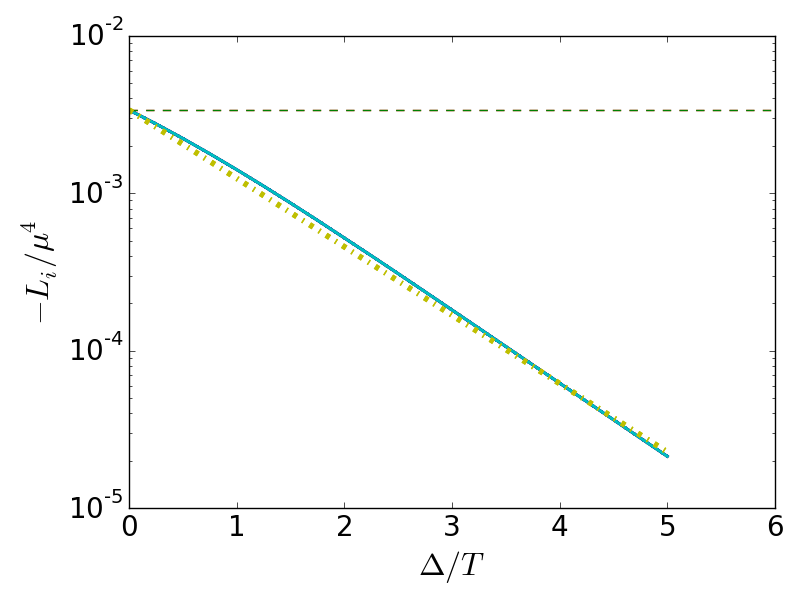
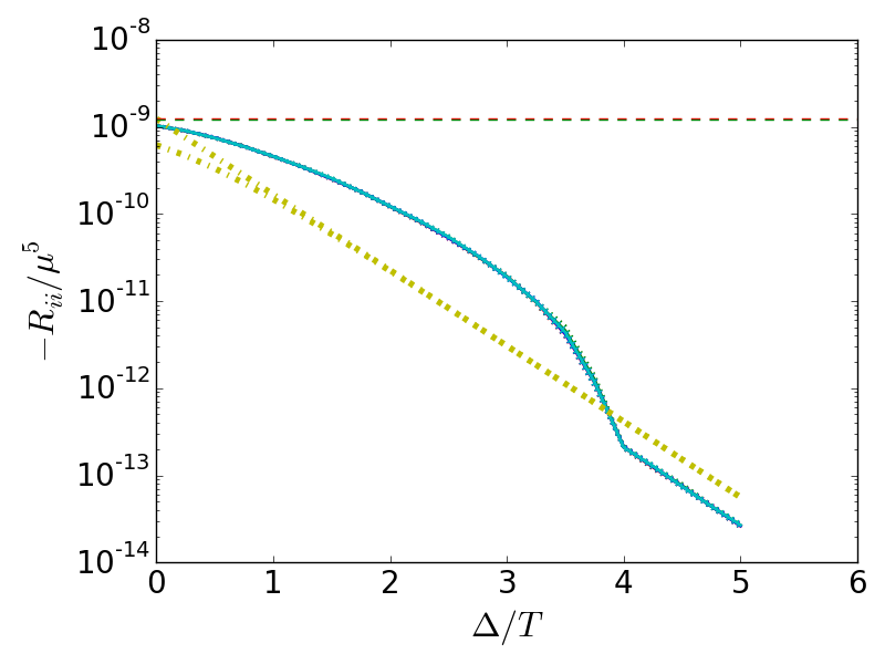
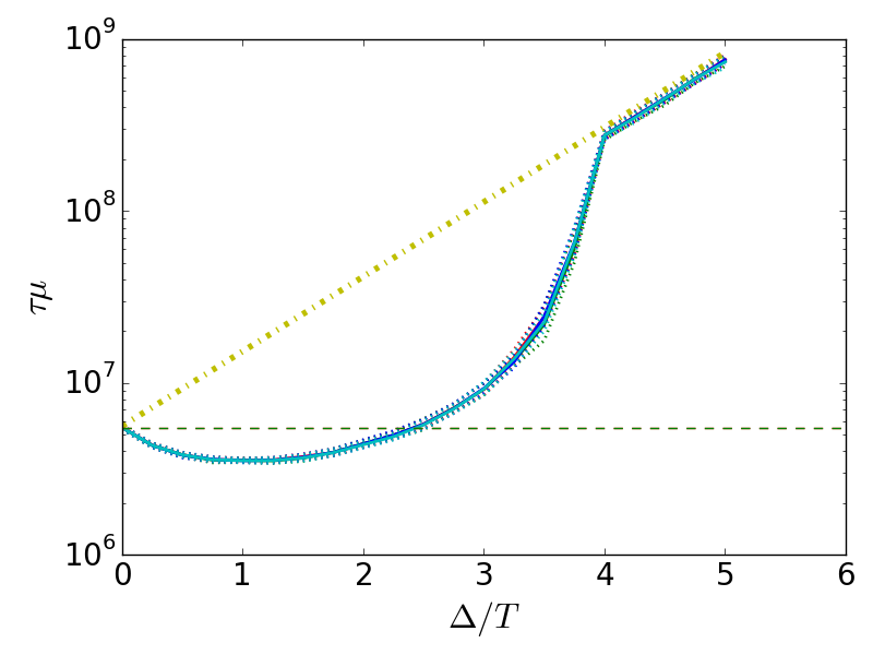
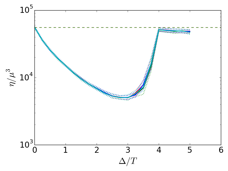
Figure 2: (color online) Plots of $L_{i}$, the diagonal entries of $R$, $\eta_{i}$ and $\tau_{i}$ (anticlockwise from top left) for $|\bar{{\cal{M}}}|^{2}$ given in Eq. 99. The overall scale is set by $\mu$. Keeping $T/\mu=3.34\times 10^{-4}$ fixed and $\delta\mu=0$, we plot these as a function of $\Delta/T$ for the “four species” $i=$, $a$, $b$, $c$, and $d$ (Eq. 46). The four solid curves [red ($a$), green ($b$), blue ($c$), and cyan ($d$) online which are indistinguishable in the plots] denote the results for the four species. The dotted curves (not visibly distinguishable in the plots) signify the errors in the numerical integration for $R$ (Eq. 133). The dashed horizontal curves (green online) are proportional to values for unpaired quarks (see text). The dot dashed curves (yellow online) show an exponential fall off, $\propto\exp(-\Delta/T)$, for $L_{i}$ (Eq. 103), an exponential fall off, $\propto\exp(-2\Delta/T)$, for $R_{ii}$ (Eq. 104), and an exponential increase, $\propto\exp(\Delta/T)$, for $\tau_{i}$. The horizontal dashed line for $L$ [$R$, $\tau$, $\eta$] corresponds to $L^{\rm{un}}/2$ (Eq. 94) [$R_{11}^{\rm{un}}$ (Eq. 96), $\tau_{1}^{\rm{un}}$ and $\eta_{1}^{\rm{un}}/2$ (Eq. 97)].  

IV.2.1 BCS pairing

We first consider the standard BCS pairing with $\delta\mu=0$. The results are shown in Fig. 2. The top left panel shows $L_{i}$ $i=a,\;b,\;c,\;d$ (Eq. 46). In this symmetric situation, $L_{i}$ are equal for all the species and are represented by four overlapping curves (red, green, blue and cyan online). Similarly, $R_{ii}$ ($i$ not summed) are all equal. (This is shown on the top right panel. We don’t show the cross terms.) Results for $\tau$ (Eq. 20) and $\eta_{i}$ (Eq. 28) are shown in the bottom left and right panel respectively.

$\Delta\rightarrow 0$— When the pairing parameter $\Delta\rightarrow 0$ ($0$ of the $x$-axis in Fig. 2), we get back a system of unpaired fermions and one should obtain the result in Sec. IV.1 in the language of Bogoliubov quasi-particles (Eq. 46).

$L_{i}$ is given by half the values given in Eq. 94 (the factor of $1/2$ arises because we restrict the integrals in $\xi$ to $\xi>0$ or $<0$ corresponding to Eq. 46)

$$\begin{split}[L](\Delta=0)=\frac{1}{2}L_{1}^{{\rm{un}}}\left(1,1,1,1\right)\end{split}$$ (100)

The dashed horizontal line (green online) on the top left panel of Fig. 2 corresponds to $L_{i}=\frac{1}{2}L_{1}^{{\rm{un}}}$ (Eq. 100, Eq. 94). A numerical evaluation of the integral for $L_{i}$ in Eq. 21 agrees with the analytic result Eq. 94 to a very high accuracy. For the collision integral, we numerically find that to a high accuracy the matrix $R_{ij}$ has the form

$$\begin{split}R_{ij}(\Delta=0)=2s_{1}^{\rm{un}}\left(\begin{array}[]{cccc}\frac{1}{2}+{\rm{f}}(\frac{T}{\mu},\frac{1}{g})&0&0&\frac{1}{2}-{\rm{f}}(\frac{T}{\mu},\frac{1}{g})\\ 0&\frac{1}{2}+{\rm{f}}(\frac{T}{\mu},\frac{1}{g})&\frac{1}{2}-{\rm{f}}(\frac{T}{\mu},\frac{1}{g})&0\\ 0&\frac{1}{2}-{\rm{f}}(\frac{T}{\mu},\frac{1}{g})&\frac{1}{2}+{\rm{f}}(\frac{T}{\mu},\frac{1}{g})&0\\ \frac{1}{2}-{\rm{f}}(\frac{T}{\mu},\frac{1}{g})&0&0&\frac{1}{2}+{\rm{f}}(\frac{T}{\mu},\frac{1}{g})\end{array}\right)\end{split}$$ (101)

(with $s^{\rm{un}}_{2}=0$ and $s^{\rm{un}}_{1}$ given in Eq. 95 ). The dashed horizontal lines (green online) on the top right panel of Fig. 2 corresponds to $R_{11}^{\rm{un}}=2s_{1}^{{\rm{un}}}$ (Eq. 101, Eq. 96).

The structure of the matrix Eq. 101 is easy to understand. The diagonal entries correspond to scattering of species $i$ with $i$. For $\Delta=0$ the branch $a$ is connected to $d$ and $b$ to $c$, and these scattering contributions are finite and they add up to $2s_{1}^{{\rm{un}}}$. In a wide range of $T\ll\mu$, ${\rm{f}}(\frac{T}{\mu},\frac{1}{g})$ is relatively insensitive to $T/\mu$ and increases with increasing $\frac{1}{g}$ (weak coupling). This is because ${\rm{f}}(\frac{T}{\mu},\frac{1}{g})$ is related to the scatterings between $a$ and $d$ (or $b$ and $c$) species which is more prominent if the scatterings that dominate the collision integral are small angle ($q\sim g\mu\ll\mu$).

Finally, the contribution to the collisional integral from scattering of particles in the branch $a$ with $b$ or $c$ is $0$ from rotational symmetry (just like $s_{2}^{{\rm{un}}}=0$ in Eq. 95). For $g=1$ in Eq. 50, ${\rm{f}}(\frac{T}{\mu},\frac{1}{g})\approx 0.32$.

From Eq. 100 and Eq. 101 one can easily obtain relaxation time $\tau_{i}(\Delta=0)=\tau_{1}^{{\rm{un}}}$ and hence the shear viscosity is $\eta_{i}=\frac{1}{2}\eta_{1}^{{\rm{un}}}$ for all four species. The total viscosity is given by

$$\eta(\Delta=0)=\sum_{i}\eta_{i}(\Delta=0)=4\eta_{i}(\Delta=0)=2\eta_{1}^{{\rm{un}}}~{}\;.$$ (102)

The dashed horizontal line (green online) on the bottom left (bottom right) panel of Fig. 2 corresponds to $\tau_{i}$ ($\eta_{i}=\eta_{1}^{{\rm{un}}}/2$) (Eq. 97).

$\Delta\gg T$— As $\Delta$ is increased, the participation of fermions in transport is thermally suppressed. Since $L_{i}$ involves single particle excitations, it is easy to see that

$$L_{i}(\Delta)\approx L_{i}(\Delta=0)e^{-\Delta/T}~{}\;.$$ (103)

This is shown in Fig. 2 by the dot-dashed curve (yellow online). Similarly, since $R_{i}$ involve two particle excitations, we expect that

$$R_{ij}(\Delta)\sim R_{ij}(\Delta=0)e^{-2\Delta/T}~{}\;.$$ (104)

We see in Fig. 2 that this turns out to be true for $\Delta/T$ larger than $4$ and the suppression for $\Delta/T\lesssim 4$ while present, is a little weaker. Consequently, one can quickly deduce that $\tau_{i}(\Delta)\sim\tau_{i}(\Delta=0)e^{\Delta/T}$: the few thermally excited quarks rarely scatter with each other. The large relaxation time compensates for the small number of momentum carrying fermions and for $\Delta/T\gtrsim 4$ the viscosity converges back to the value for unpaired quark matter.

This result is puzzling since we expect the paired fermions to be frozen at temperatures smaller than the pairing gap and hence not contribute to the viscosity. We expect only the low energy phonons to participate in transport at low energies Rupak and Schäfer (2007).

We argued in the previous section (Sec. IV.1) that in the absence of pairing for $T\ll\mu$, the contribution to the quark collision integral $R$ from quark-phonon scattering (Eq. 96) is sub-dominant to the contribution from quark-quark scattering (Eq. 85). Pairing, however, affects these two contributions differently. Since quark-phonon scattering involves only one gapped mode, we expect the $R_{ij(q-{\rm{ph}})}(\Delta)\sim R_{ij(q-{\rm{ph}})}(0)e^{-\Delta/T}$ rather than as in Eq. 104 and dominates scattering. Then $\tau_{i}$ doesn’t grow exponentially and $\eta_{i}$ is exponentially suppressed.

More systematically, for $\Delta\gg T$

$$\begin{split}L_{i}\approx\frac{-2}{15}\frac{\mu^{4}}{(2\pi)^{2}}e^{-\Delta/T},\;\;\;\;\;\;{i=a,b,c,d}~{}\end{split}$$ (105)

and (Eqs. 104, 85),

$$\begin{split}R_{ii}(\Delta)\approx&[-\frac{1}{2}\frac{g^{3}T^{2}\mu^{3}\nu}{640\pi\sqrt{2}}e^{-2\Delta/T}-c\mu T^{4}e^{-\Delta/T}]\\ \approx&-c\mu T^{4}e^{-\Delta/T}\;\;\;\;\;\;{i=a,b,c,d}~{}\end{split}$$ (106)

where we have taken $\Pi_{l}(0)=(g\mu/(2\pi))^{2}$ and $c$ is a number ${\cal{O}}(1)$. Hence,

$$\begin{split}\tau_{i}\approx\frac{2c}{15(2\pi)^{2}}\frac{\mu^{3}}{T^{4}}\;\;\;\;\;\;{i=a,b,c,d}\;.~{}\end{split}$$ (107)

Therefore, the fermionic contribution to the shear viscosity is given by

$$\begin{split}\eta_{i}=-3\tau_{i}L_{i}\approx\frac{4}{75(2\pi)^{4}}\frac{\mu^{7}}{T^{4}}e^{-\Delta/T}\;\;\;\;\;\;{i=a,b,c,d}\;,~{}\end{split}$$ (108)

which is subdominant to the phonon contribution (Eq. 88, since we are assuming no other gapless fermions are present).

This entire argument relies on the existence of a gapless mode in the low energy theory, but in most of the paired systems we know such a mode is present. If the symmetry broken by the fermion condensate is global or has a global component  then the pairing itself gives rise to a Goldstone mode which can scatter off fermions. If the symmetry broken by the condensate is local rather than global, then pairing does not by itself give rise to a phonon mode. For example in ordinary BCS superconductors the local $U(1)\rightarrow Z_{2}$ gives a mass to the transverse photons (the Meissner effect). However even in this case there is a Goldstone mode associated with the breaking of translational symmetry by the underlying lattice.  

Therefore the common statement that the paired fermions don’t contribute to transport at low temperatures is generically true, but subtle. Things are cleaner if there are fermionic modes that are gapless, in which case they dominate transport when $\mu\gg T$. This is the situation we shall explore next.

In drawing Figs. 2 we have taken $g=1$. Obtaining results for arbitrary $g$ is simple. The top left panel ($L_{i}$) doesn’t depend on the collisions and is not modified. The square of the matrix element, $|{\cal{M}}|^{2}$, scales as ${g^{4}}$ and $\sqrt{\Pi_{l}}$ scales as $g$. Consequently $\tau_{i}$ and $\eta_{i}$ scale as ${1}/{g^{3}}$.

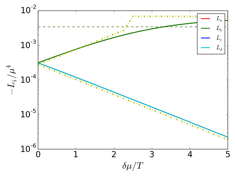
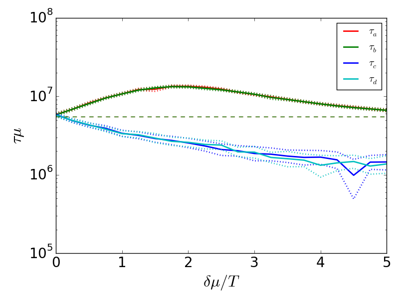
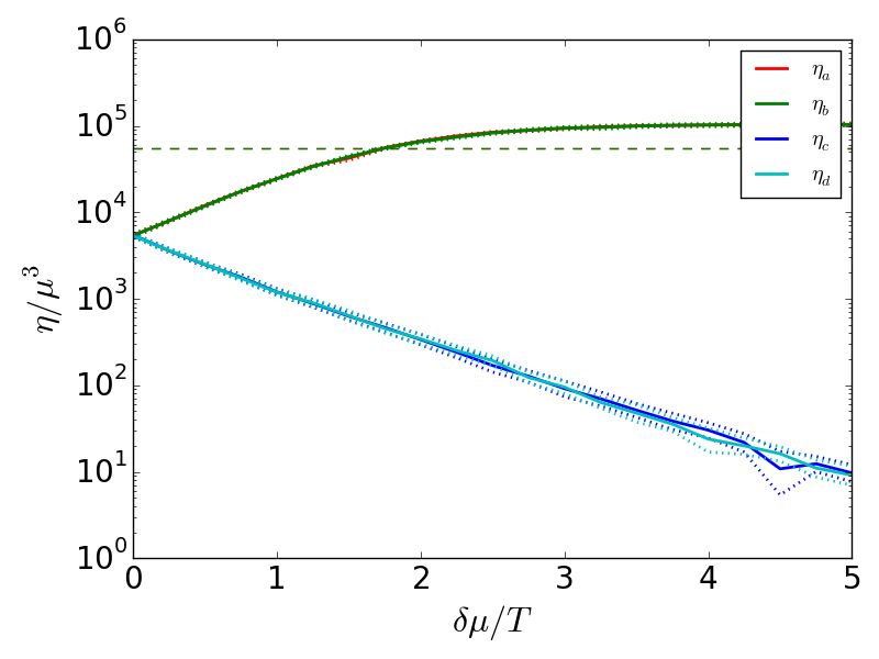
Figure 3: (color online) Plots of $L_{i}$, the diagonal entries of $R$, $\eta_{i}$ and $\tau_{i}$ (anticlockwise from top left) with $|\bar{{\cal{M}}}|^{2}$ given in Eq. 99 for the four species $a$, $b$, $c$, and $d$ (Eq. 46). The dashed horizontal lines correspond to the values for unpaired matter (see the caption of Fig. 2 for details). The pairing is isotropic (${\bf{b}}=0$). $T/\mu=3.34\times 10^{-4}$ and $\Delta/T=2.5$ are held fixed, and $\delta\mu$ is varied from $0$ to $2\Delta$. For $\Delta>\delta\mu$ ($\delta\mu/T<2.5$ in all the plots) all fermionic excitations are gapped and all components of $R$ are exponentially suppressed. For $\Delta<\delta\mu$, branches $a$ and $b$ feature gapless fermionic excitations. The asymptotic value ($\delta\mu\gg\Delta$) for $\eta_{a}=\eta_{b}=2\eta^{\rm{un}}_{1}$. The dot dashed curves (yellow online) for $L$ are the simple forms given in Eq. 110 for $\delta\mu>\Delta$, and Eq. 109 for $\delta\mu<\Delta$. The error bands are shown by the dashed curves of the color of the corresponding solid curves, and are associated with errors in the five dimensional Monte Carlo integration used for evaluating $R_{ij}$ (Eq. 133). $\tau_{c}$, $\tau_{d}$ are noisy but don’t affect the final result for $\eta$.  

IV.2.2 Isotropic gapless pairing

To analyze the effect of gapless fermions in this simple system let us consider an isotropic gapless paired phase (${\bf{b}}\rightarrow 0$, $\Delta>\delta\mu$). As discussed in Sec. II, this phase is unstable, but the analyses will give us insight into the anisotropic calculation. In Fig. 3 we keep $\Delta>T$ fixed ($\Delta/T=2.5$), and consider the effect of increasing $\delta\mu$ keeping $b$ equal to $0$.

Based on the discussion in Sec. IV.2.1, we expect that for $\Delta>\delta\mu$ both $L_{i}$ and $R_{ij}$ to be exponentially suppressed from the unpaired value. Whereas for $\Delta<\delta\mu$ (Eq. 42) $E_{1}=0$ for $\xi=\pm\sqrt{\delta\mu^{2}-\Delta^{2}}$ and therefore the branches $a$ and $b$ in Eq. 46 are gapless while the branches $c$ and $d$ are gapped. Therefore, for $\delta\mu>\Delta$ we expect $L_{i}$, and $R_{ij}$ corresponding $a$ and $b$ to be unsuppressed compared to the unpaired value.

More specifically, for $\Delta-\delta\mu\gg T$

$$\begin{split}L_{a,b}(\Delta,\delta\mu)&\approx\frac{1}{2}L_{1}^{{\rm{un}}}e^{-\frac{(\Delta-\delta\mu)}{T}}=L_{a}(\Delta=0,\delta\mu=0)e^{-\frac{(\Delta-\delta\mu)}{T}}\\ L_{c,d}(\Delta,\delta\mu)&\approx\frac{1}{2}L_{1}^{{\rm{un}}}e^{-\frac{(\Delta+\delta\mu)}{T}}=L_{a}(\Delta=0,\delta\mu=0)e^{-\frac{(\Delta+\delta\mu)}{T}}~{}\;.\end{split}$$ (109)

In the top left panel of Fig. 3, the curves for $L_{i}$ for the $a$ and $b$ branches (red and green online) split from the $c$ and $d$ branches (blue and cyan online) on switching on a small $\delta\mu$. The splitting increases as we increase $\delta\mu$ and for $\delta\mu-\Delta\gg T$, near the gapless surfaces $\xi=\pm\sqrt{\delta\mu^{2}-\Delta^{2}}$, both $a$ and $b$ branches resemble unpaired fermions. Therefore,

$$\begin{split}L_{a,b}(\Delta,\delta\mu)_{\delta\mu\gg\Delta}&\rightarrow L_{1}^{{\rm{un}}}=2L_{a}(\Delta=0,\delta\mu=0)\\ L_{c,d}(\Delta,\delta\mu)&\approx\frac{1}{2}L_{1}^{{\rm{un}}}e^{-\frac{(\Delta+\delta\mu)}{T}}~{}\;.\end{split}$$ (110)

The limiting behaviors Eq. 109 and Eq. 110 are shown by dot dashed curves (yellow online) on the top left panel of Fig. 3.

Similarly, for $\Delta-\delta\mu\gg T$ we expect $R_{ii}$ for each $i$ to be suppressed compared to $R^{{\rm{un}}}_{ii}$. For example, for $\delta\mu=0$, we see that for $\Delta/T=2.5$, $R_{ii}(\Delta=2.5T,\delta\mu=0)\approx R^{{\rm{un}}}_{ii}/15$. The suppression factor of $15$ is consistent with $R_{ii}(\Delta=2.5T,\delta\mu=0)/R^{{\rm{un}}}_{ii}$ in Fig. 2.)

As $\delta\mu$ is increased, the gapless branches $a$ (green online), $b$ (red online) split from $c$ (blue online) and $d$ (cyan online), and eventully for $\delta\mu-\Delta\gg T$

$$\begin{split}R_{aa,bb}(\Delta,\delta\mu)|_{\delta\mu\gg\Delta}\rightarrow R_{1}^{{\rm{un}}}\end{split}$$ (111)

the top right panel of Fig. 3 shows this behavior clearly. $R_{cc,dd}(\Delta,\delta\mu)\sim R_{1}^{{\rm{un}}}\exp(-2(\Delta+\delta\mu)/T)$. The off-diagonal terms of $R$ are also exponentially suppressed.

This pattern is repeated for $\tau$ and $\eta$: $\tau_{a}$ ($\eta_{a}$), $\tau_{b}$ ($\eta_{b}$) tend towards $\tau_{1}^{\rm{un}}$ ($\eta_{1}^{\rm{un}}$) for $\delta\mu-\Delta\gg T$ while $\tau_{c}$ ($\eta_{c}$), $\tau_{d}$ ($\eta_{d}$) are weakly (exponentially) suppressed. All this is just a complicated way to obtain the well understood result (for eg. see Ref. Alford et al. (2005a)) that the transport in gapless superfluids is dominated by fermionic modes near the gapless surfaces (Eq. 12) and the result for the total viscosity in the limit $\delta\mu-\Delta\gg T$ is the same as for an unpaired system,

$$\eta(\delta\mu\gg\Delta)=\sum_{i}\eta_{i}\approx\eta_{a}+\eta_{b}\approx 2\eta_{1}^{{\rm{un}}}~{}\;.$$ (112)

In light of the simple and intuitive result Eq. 112, the analysis of this section seems needlessly complicated: one could restrict to modes near the gapless spheres (mode $a$ near $\xi=-\sqrt{\delta\mu^{2}-\Delta^{2}}$ and mode $b$ near $\xi=+\sqrt{\delta\mu^{2}-\Delta^{2}}$) and neglect modes $c$ and $d$. Near the gapless $\xi$, the dispersion of the modes can be approximated as linear, which means that standard Fermi liquid techniques would lead to Eq. 112 for gapless fermions if $\delta\mu\gg\Delta$.

While the discussion of the isotropic gapless phase clarifies some aspects of the calculation of the collision integrals for the FF phase, the details of the analysis is more subtle because the pairing pattern is anisotropic. In the following section we present the results for anisotropic pairing.

V Results for anisotropic pairing

From the dispersions Eq. 43, one can think of the problem in terms of an angle dependent Fermi surface splitting,

$$\delta\mu_{\rm{eff}}(\cos\theta)=\delta\mu+b\cos\theta\;.$$ (113)

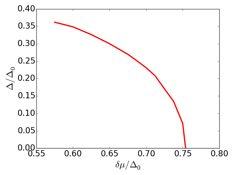
Figure 4: (color online) Plot of $\Delta/\Delta_{0}$ versus ${\delta\mu}/\Delta_{0}$ for $b=\zeta\delta\mu$ from Mannarelli et al. (2006). $\Delta_{0}$ is the gap for the $2{\rm{SC}}$ phase in the absence of the Fermi surface split. At $\delta\mu=0.754\Delta_{0}$, $\Delta=0$.  

For $\delta\mu+b\cos\theta>\Delta$, species $a$ and $b$ are gapless, for $\Delta>\delta\mu+b\cos\theta>-\Delta$ all four modes are gapped, and for $\delta\mu+b\cos\theta<-\Delta$ modes $c$ and $d$ are gapless (Eq. 43) Alford et al. (2001b); Bowers (2003). Therefore, the shape of the gapless surface depends on the values of $\delta\mu$ and the gap parameter $\Delta$ which is a function of $\delta\mu$. Furthermore, even the nature of the gapless modes changes with the angle depending upon whether $|\delta\mu_{\rm{eff}}(\cos\theta)|\gg\Delta$ (in which case the dispersion near the gapless modes is linear and the mode velocity $v\approx 1$) or $|\delta\mu_{\rm{eff}}(\cos\theta)|\approx\Delta$ (in which case the dispersion near the gapless modes is quadratic and the mode velocity $v\approx 0$). Consequently, the results for the FF phase can not be obtained by a simple extension of the isotropic analysis and a detailed calculation of the collision integral is necessary. We perform this analysis for a simple model for quark interactions: exchange of Debye screened, longitudinal gluons described by Eqs. 79 90, in the next section (Sec. V.1). In Sec. V.2 we show the analysis for the two-flavor FF phase with the realistic interaction: exchange of dynamically screened, transverse $t^{1}$, $t^{2}$, and $t^{3}$ gauge bosons.

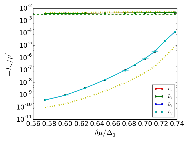
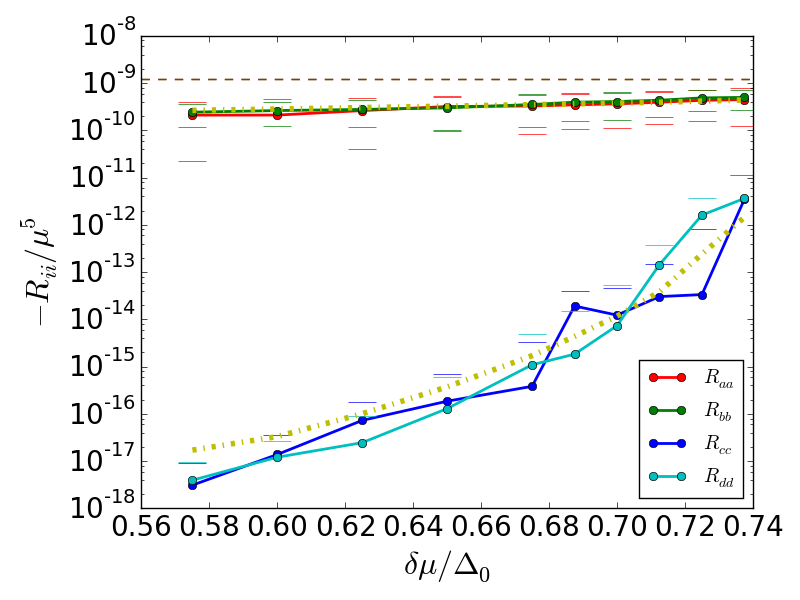
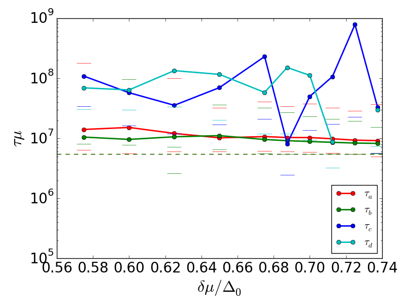
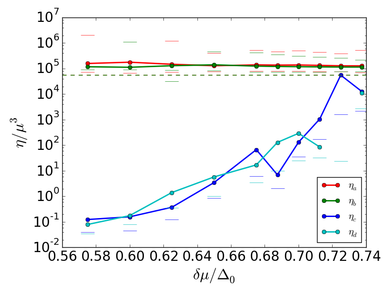
Figure 5: (color online) Plots of $L_{i}$, the diagonal entries of $R$, $\eta_{i}$ and $\tau_{i}$ (anticlockwise from top left) with $|\bar{{\cal{M}}}|^{2}$ given in Eq. 99 for the four species $a$, $b$, $c$, and $d$ (Eq. 46). The pairing is anisotropic with $b=1.19\delta\mu$ and $\Delta$ is taken from Fig. 4. $T/\mu=3.34\times 10^{-4}$ is held fixed and $T/\Delta_{0}=0.02$. The central values are given by filled circles and the error bars are are shown by the dashes of the corresponding color. The error bars for $R_{ij}$ are associated with errors in the seven dimensional Monte Carlo integration used for evaluating $R_{ij}$ (Eq. 134) and are propagated to $\tau$ and $\eta$. The large errors in $\tau_{c}$ and $\tau_{d}$ (blue and cyan online) do not affect the final $\eta$. The dashed horizontal lines correspond to the values for unpaired matter (see the caption of Fig. 2 for details). The upper dot dashed curves in the panels for $L_{a}$ and $L_{b}$ ($R_{aa}$, $R_{bb}$) [yellow online] are associated with geometric reduction due to a smaller gapless surface as described in Eq. 115 (Eq. 116). The lower dot dashed curves in the panels for $L_{c}$ and $L_{d}$ ($R_{cc}$, $R_{dd}$) [yellow online] are associated with exponential reduction due to pairing. The results are discussed from Eqs. 115 to Eq. 118 in the text.  

V.1 Debye screened gluon exchange

To evaluate the integrals $L_{i}$ and $R_{ij}$ appearing in Eq. 21 with the dispersions Eq. 43 for any given $T$ and $\delta\mu$, we need $\Delta$ and $b$ as a function of $\delta\mu$. For a given $b$ and $\delta\mu$, $\Delta$ can be found by solving the gap equation for the FF phase Mannarelli et al. (2006).

We take the solution of the gap equation, $\Delta$ as a function of $\delta\mu$, from Fig. $3$ in Ref. Mannarelli et al. (2006). The calculations in Ref. Mannarelli et al. (2006) were performed for three-flavor pairing with an FF pairing pattern for $ud$ and $sd$ pairing. When the angle $\phi$ between the two plane waves is $0$, the two pairing rings on the $u$ interfere minimally and hence we use the corresponding solution to the gap equation (green curve in Fig. $3$ in Ref. Mannarelli et al. (2006)), reproduced in Fig. 4.

Near the second order phase transition at $\delta\mu<0.754\Delta_{0}$, $\Delta/\Delta_{0}\ll 1$ and $b=\zeta\delta\mu$ minimizes the free energy. Here, $\Delta_{0}$ is the gap in the $2{\rm{SC}}$ phase in the absence of Fermi surface splitting and the precise value of $\zeta$ is $1.1996786...$ Larkin and Ovchinnikov (1964); Fulde and Ferrell (1964); Bowers and Rajagopal (2002); Bowers (2003); Mannarelli et al. (2006). $\Delta$ is zero at the transition and increases with decreasing $\delta\mu$ Fig. 4. In this paper we will use $b/\delta\mu=1.19$ for the entire range $\delta\mu/\Delta_{0}\in(0.575,0.75)$.

Even though the FF phase is not favoured compared to the homogeneous pairing phase (in which the paired fermions are gapped since $\Delta=\Delta_{0}>\delta\mu$) for $\delta\mu<0.707\Delta$, we will explore this range because of the possibility that the higher plane wave states may be favoured in a wider region and may be governed by similar physics. (Also see Ref. Leibovich et al. (2001).)

In Fig. 5 we plot the results for $L$, $R$, $\tau$ and $\eta$ as a function of $\delta\mu$ with $b$ and $\Delta$ chosen as described above. For a fixed $\mu$, which sets the overall scale, there are two dimensionless ratios that are needed to specify the transport properties of the FF phase as a function of $\delta\mu$, $T/\mu$, and $\Delta_{0}/\mu$. We show the results for $T/\mu=3.34\times 10^{-4}$ and $\Delta_{0}/\mu=1.67\times 10^{-2}$ in Fig. 5 though the results should be unchanged as long as the hierarchy of scales $T\ll\Delta_{0}$ and $\Delta_{0}\ll\mu$ are satisfied.

To get a concrete feel for numbers, one can take $\mu=300$MeV, $\Delta_{0}=5$MeV (which is on the lower edge of $\Delta_{0}$ for model studies) and $T=0.1$MeV. We choose $\Delta_{0}=5$MeV so that the exponential suppression $\exp(-\Delta/T)$ is small enough to be clearly visible in the results, but still large enough to be accessible within numerical errors.

First considering $L_{i}$ (top left panel of Fig. 5) as a function of $\delta\mu$, we note that the branches $a$ and $b$ are gapless for

$$\begin{split}\cos\theta\in[\frac{-\delta\mu+\Delta}{b},1]~{}\end{split}$$ (114)

throughout the range $\delta\mu/\Delta_{0}\in(0.575,0.75)$ (Appendix A). The gapless surface is the boundary of a crescent with arc-length $1+\frac{\delta\mu-\Delta}{b}$ instead of $2$. Therefore, we expect $L_{a}=L_{b}=L^{{\rm{un}}}\times{\rm{g}}(\frac{\delta\mu}{b},\frac{\Delta}{b})$ where ${\rm{g}}$ is a dimensionless function smaller than $1$ corresponding to the limited range for which the modes are gapless. The following geometric estimate turns out to be reasonably accurate

$$\begin{split}L_{a}=L_{b}&\approx L^{{\rm{un}}}\times\frac{1}{2}(1+\frac{\delta\mu}{b}-\frac{\Delta}{b})~{}\;.\end{split}$$ (115)

This is shown by the upper dot dashed line (yellow online).

On the other hand, the branches $c$ and $d$ are gapped for $\delta\mu/\Delta_{0}<0.735$ and hence $L_{c}$ and $L_{d}$ are exponentially suppressed. A rough estimate is $L_{c}=L_{d}\sim e^{-\Delta/T}$. The lower dot dashed curve (yellow online) is $L^{{\rm{un}}}e^{-\Delta/T}$ and shows the right form up to a scale. The proportionality factor depends upon $T$.

Similarly, $R_{ij}$ is expected to be suppressed by the square of the phase space factor,

$$\begin{split}R_{aa}=R_{bb}&\approx\frac{1}{2}R^{{\rm{un}}}_{11}\times(\frac{1}{2}(1+\frac{\delta\mu}{b}-\frac{\Delta}{b}))^{2}~{}\;.\end{split}$$ (116)

This is shown by the upper dot dashed line (yellow online) on the top right panel of Fig. 5. $R_{cc}$ and $R_{dd}$ are exponentially suppressed and their evaluation is noisy (see Appendix B for details). However, a reasonable estimate is $R_{cc}=R_{cc}\approx R^{{\rm{un}}}_{11}\times e^{-\Delta/T}$. We stop the results for $\delta\mu/\Delta_{0}=0.74$ since for larger $\delta\mu$, $\Delta\rightarrow 0$ and the numerical evaluation of the integral is noisy.

From Eqs. 115 and  116 we expect,

$$\begin{split}\tau_{a}&=\tau_{b}\approx 2\tau^{{\rm{un}}}\\ \eta_{a}&=\eta_{b}\approx\eta^{{\rm{un}}}~{}\;.\end{split}$$ (117)

$\tau_{c}$ and $\tau_{d}$ are noisy but do not contribute significantly to the final $\eta$ and can be ignored.

Consequently,

$$\eta(b\neq 0)=\sum_{i}\eta_{i}\approx\eta_{a}+\eta_{b}\approx 2\eta_{1}^{{\rm{un}}}~{}\;.$$ (118)

This is a remarkable result and is once again a consequence of the intricate interplay between $\tau$ and $\eta$ that we saw in Sec. IV.2.1. The reduced phase space due to pairing increases $\tau_{a}$ and $\tau_{b}$ by the same factor as it decreases $L_{a}$ and $L_{b}$ because $R$ goes as the square of this factor. Consequently, in the product, the two effects cancel out.

The key results that we obtained in this section are that

1. $L_{a}$ and $L_{b}$ are only geometrically suppressed by the smaller gapless surface (Eq. 115)

2. $L_{c}$ and $L_{d}$ are exponentially suppressed

3. For Debye screened mediators, $R_{aa}$ and $R_{bb}$ are only geometrically suppressed (Eq. 116)

4. $R_{cc}$ and $R_{dd}$ are exponentially suppressed

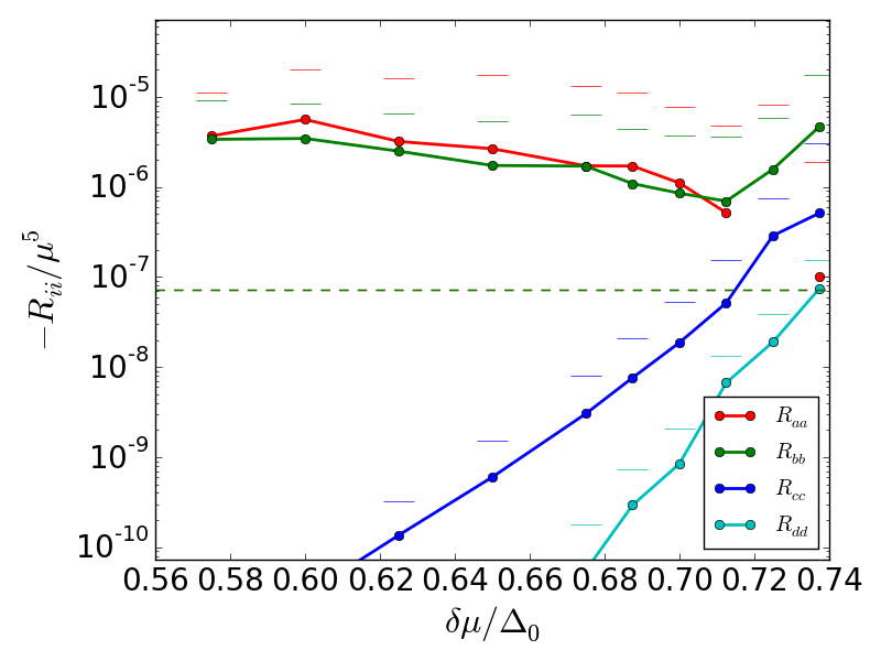
Figure 6: (color online) Plots of the diagonal entries of $R$ for the four species $a$, $b$, $c$, and $d$ (Eq. 46) with $|\bar{{\cal{M}}}|^{2}$ given by Eq. 119. The pairing is anisotropic with $b=1.19\delta\mu$ and $\Delta$ is taken from Fig. 4. $T/\mu=3.34\times 10^{-4}$ is held fixed and $T/\Delta_{0}=0.02$ (the same as in Fig. 5). The central values are given by filled circles and the error bars (from the Monte Carlo integration for $R$) are are shown by the dashes of the corresponding color. The dashed horizontal line corresponds to $R_{11}$ for unpaired matter with the interaction specified by Eqs. 51, 52.

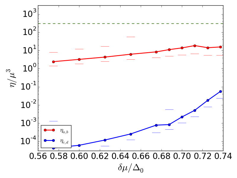
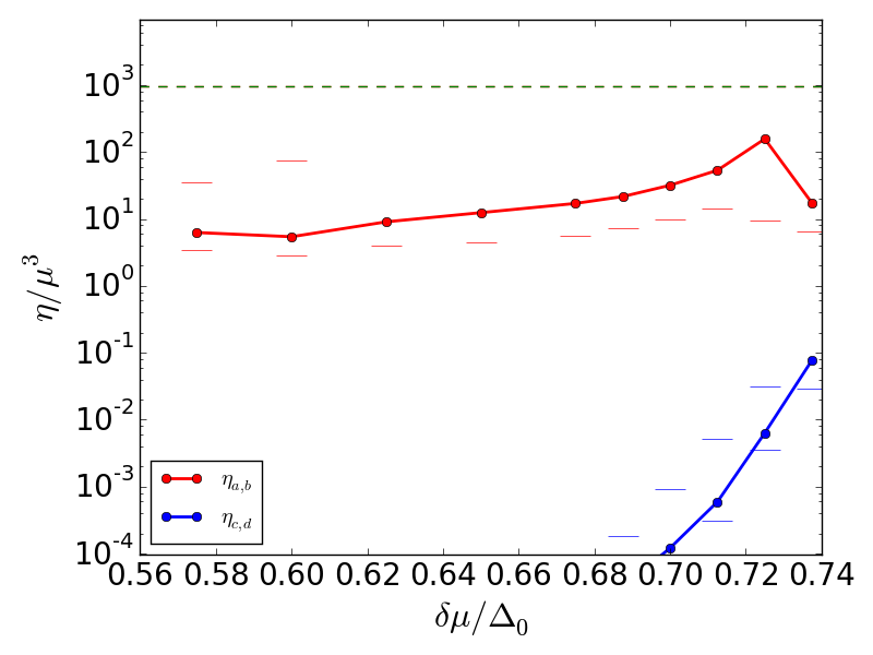
Figure 7: (color online) Plots of $\eta_{i}$ (anticlockwise from top left) for the four species $a$, $b$, $c$, and $d$ (Eq. 46) for anisotropic pairing with ${\bf{b}}=1.19\delta\mu$. $T/\mu=3.34\times 10^{-4}$ is held fixed and $T/\Delta_{0}=0.025$, $T/\Delta_{0}=0.05$, $T/\Delta_{0}=0.1$, $T/\Delta_{0}=0.2$.  

V.2 Two-flavor FF phase using $t^{1}$, $t^{2}$, $t^{3}$ exchange

Now we use the interaction mediated by the Landau damped $t^{1}$, $t^{2}$, $t^{3}$ to calculate $\eta$ in the two-flavor FF phase. In the Eq. 21 the left hand sides, $L_{i}$, depend only on the spectrum of quasi-particles and not the interaction. Therefore, they are not modified. For $T/\Delta_{0}=0.02$ they are as shown in the top left panel of Fig. 5 in Sec. V.1.

The difference from Sec. V.1 appears in the collision integral $[R_{ij}]$, where the square of the matrix element $|{\cal{M}}(12\rightarrow 34)|^{2}$ in Eq. 21 (or Eq. 134) is given by Eq. 75 instead of Eq. 99. As discussed in Sec. III.4, the matrix element in the collision integral is (Eq. 75)

$$\begin{split}|i\bar{\cal{M}}|^{2}&=3(\frac{g}{2})^{4}\delta_{i_{2}i_{4}}\delta_{i_{1}i_{3}}\\ &\frac{1}{4}\frac{1}{2p_{1}2p_{2}2p_{3}2p_{4}}{\rm{tr}}[p\!\!\!/_{3}\gamma^{\mu}p\!\!\!/_{1}\gamma^{\nu}]{\rm{tr}}[p\!\!\!/_{4}\gamma^{\sigma}p\!\!\!/_{2}\gamma^{\lambda}]{D}_{\mu\sigma}{D}_{\nu\lambda}~{}\;.\end{split}$$ (119)

Evaluating the Dirac traces we obtain,

$$\begin{split}|\bar{{\cal{M}}}|^{2}&=3\bigl{(}\frac{g}{2}\bigr{)}^{4}\Bigl{(}L_{t}^{xx}\frac{1}{|{\bf{q}}^{2}-w^{2}+\Pi^{xx}_{t}|^{2}}+L_{t}^{yy}\frac{1}{|{\bf{q}}^{2}-w^{2}+\Pi^{yy}_{t}|^{2}}\\ &+2\Re e[L_{t}^{xy}\frac{1}{{\bf{q}}^{2}-w^{2}+\Pi^{xx}_{t}}\frac{1}{{\bf{q}}^{2}-w^{2}+(\Pi^{yy}_{t})^{*}}]\Bigr{)}\;,~{}\end{split}$$ (120)

where,

$$\begin{split}L_{t}^{xx}&=(\cos(\phi_{1})\cos(\phi_{2}))^{2}\\ L_{t}^{yy}&=(\sin(\phi_{1})\sin(\phi_{2}))^{2}\\ L_{t}^{xy}&=\frac{1}{4}(\sin(2\phi_{1})\sin(2\phi_{2}))\\ L_{t}^{yx}&=L_{t}^{xy}\;,~{}\end{split}$$ (121)

and $\Pi^{xx}_{t}$, $\Pi^{yy}_{t}$ are specified by Eqs. 61 62. In an isotropic system $\Pi^{xx}_{t}=\Pi^{yy}_{t}=\Pi$ for which Eq. 120 matches the expressions in Refs. Heiselberg and Pethick (1993); Alford et al. (2014).

Before exploring the main results of anisotropic pairing with anisotropic Landau damping, we quickly review well known results for the the simpler unpaired system. For isotropic Landau damping (Eq. 52) a rough estimate Heiselberg and Pethick (1993); Alford et al. (2014) is

$$\begin{split}\frac{R_{11}^{t\;{\rm{un}}}}{R_{11}^{{\rm{un}}}}&\approx 3\bigl{(}\frac{4\sqrt{2}g\mu}{\pi^{2}T}\bigr{)}^{1/3}~{}\;,\end{split}$$ (122)

where $R_{11}^{{\rm{un}}}$ is given by Eq. 96. For $T/\mu=3.34\times 10^{-4}$ and $g=1$ the estimated enhancment factor is numerically about $36$. Evaluating the collision integral numerically, one obtains $R_{11}^{t\;{\rm{un}}}/\mu^{5}\approx-7.2\times 10^{-8}$ shown by the dashed horizontal line (green online) in Fig. 6 . Comparing with the numerical result for the longitudinal gluon exchange, $R_{11}^{{\rm{un}}}/\mu^{5}\approx-1.23\times 10^{-9}$ from the dashed horizontal line in (green online) on the top right column of Fig. 5, we see that numerically the enhancement factor is $\sim 58$, which shows that the estimate (Eq. 122) is in the right ballpark. This also impies we can ignore the longitudinal gluons. This also applies to the FF phase.

The non-trivial results shown in Fig. 6 are the values of $R_{aa}$ and $R_{bb}$ for the FF phase. The pairing is anisotropic with $b=1.19\delta\mu$ and $\Delta$ is taken from Fig. 4. $T/\mu=3.34\times 10^{-4}$ is held fixed and $T/\Delta_{0}=0.02$ (the same as the parameters used in Fig. 5). The geometric suppression due to the smaller gapless surface (Eq. 116) would lead to a reduction in $R_{aa}$ and $R_{bb}$. The actual numerical evaluation for $R_{aa}$ and $R_{bb}$ shows that they are enhanced over the unpaired isotropic result. This can be understood as follows.

For small ${\bf{q}}$,

$$\begin{split}E_{{\bf{p}}_{3}}-E_{{\bf{p}}_{1}}&\approx\frac{dE_{{\bf{p}}_{1}}}{d\xi_{p_{1}}}\delta\xi_{p_{1}}+\frac{dE_{{\bf{p}}_{1}}}{d\cos\theta_{p_{1}}}\delta\cos\theta_{p_{1}}\approx v_{p_{1}}\delta\xi_{p_{1}}~{}\;,\end{split}$$ (123)

where

$$\begin{split}v_{p_{1}}&=\frac{dE_{{\bf{p}}_{1}}}{d\xi_{p_{1}}}=\frac{\xi_{{\bf{p}}}}{\sqrt{\xi_{{\bf{p}}}^{2}+\Delta^{2}}}\;,\;\;\delta\xi_{p_{1}}=|{\bf{p}}_{1}+{\bf{q}}|-|{\bf{p}}_{1}|\;.\end{split}$$ (124)

Therefore, the energy conserving $\delta$ functions can be approximately written as $\delta({v_{p_{1}}}\delta\xi_{p_{1}}-\omega)\delta(-{v_{p_{2}}}\delta\xi_{p_{2}}-\omega)$. For $|\delta\mu+b\cos\theta|\approx\Delta$, the dispersion is gapless for $\xi\approx 0$ (Eq. 129) implying $v_{p}\rightarrow 0$ and the jacobian for the $\delta$ functions diverges. Higher order terms in the Taylor expansion of $\xi_{p}$ prevent $R_{ij}$ from diverging, but this shows up as an increase in $R_{ij}$. A similar phenomenon for the isotropic gapless CFL phase was seen earlier in Ref. Alford et al. (2005b).

There are two reasons why this effect is not seen in Fig. 5 where the interaction is mediated by Eq. 90. First, the relative $-$ sign between the coherence factor in Eq. 99 compared with the $+$ sign in Eq. 75 implies that the matrix element Eq. 99 tends to $0$ if $\xi\rightarrow 0$ while Eq. 75 does not (we also discussed a similar effect in Sec. III.4). Second, this effect is more important if the collision integral is dominated by small ${\bf{q}}$ compared to $\mu$ and the linear expansion (Eq. 123) is accurate: The effect is therefore more pronounced where the exchanged gauge boson is Landau damped. 

With the collision integral $R$ in hand, we can calculate $\tau$ and $\eta$. The results for $\eta$ for four different values of the temperatures, $T/\Delta_{0}=0.025$, $T/\Delta_{0}=0.05$, $T/\Delta_{0}=0.1$, $T/\Delta_{0}=0.2$, are shown in Fig. 7 and clearly show a reduction in $\eta$ by a factor of roughly $100$ associated with the enhancement in the collision integral.

One technical comment about the numerical evaluation is that because of the more peaked nature of the integrand due to the two reasons mentioned above, the Monte Carlo integration for $R_{ij}$ (Eq. 134) converges very slowly. Therefore to improve the statistics, we have averaged $R_{aa}$ and $R_{bb}$ (which should be equal), and $R_{ab}$ and $R_{ba}$ (which should be equal) while making Fig. 7 and added the errors in quadrature. Similarly, we have combined the data for the $c$ and $d$ branches in Fig. 7

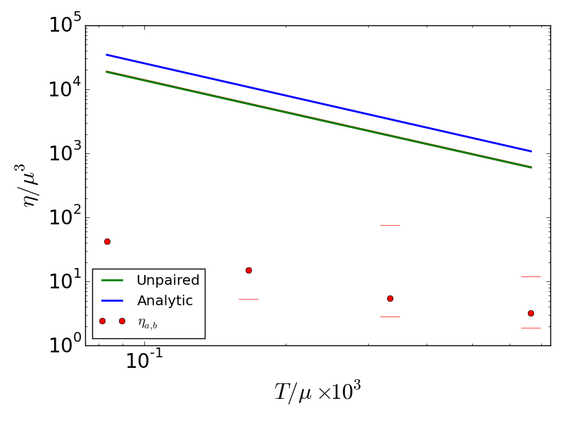
Figure 8: (color online) $\eta_{i}$ for species $a$ and $b$ for anisotropic pairing with $\Delta/\Delta_{0}=0.35$, $\delta\mu/\Delta_{0}=0.6$, and ${\bf{b}}=1.19\delta\mu$ as a function of $T$. The viscosities are obtained from Fig. 7.  

Fig. 8 shows viscosity as a function of $T$ for anisotropic phases for $\delta\mu/\mu=10^{-2}$. The blue curve is the analytic estimate

$$\begin{split}\eta^{t\;{\rm{un}}}_{1}=\eta_{1}^{{\rm{un}}}\frac{1}{3}\bigl{(}\frac{4\sqrt{2}g\mu}{\pi^{2}T}\bigr{)}^{-1/3}~{}\end{split}$$ (125)

based on Eq. 122, where $\eta_{1}^{{\rm{un}}}$ is given in Eq. 97.

The green curve is the numerical evaluation of the viscosity in the unpaired phase using Eq. 133. The result for the FF phase is denoted by the solid points with errors denoted by error bars. The error bars are large enough that we do not attempt a fit but a rough description of the data in this $T$ range is given by

$$\begin{split}\eta\sim 10^{-2}\eta^{t\;{\rm{un}}}_{1}~{}\;.\end{split}$$ (126)

Since $\eta$ is relatively flat with respect to $\delta\mu$ for all the $T$’s in a wide range of $T\ll\Delta$ (Fig. 6), we propose Eq. 126 as a fair parameterization of the shear viscosity in the FF phase for $T\ll\Delta$ throughout the two-flavor FF window. Eq. 126 is a concise summary of our main result.

VI Conclusions

We present the first calculation of the shear viscosity of the two-flavor FF phase of quark matter.

We identify the low energy quasi-particles that play an important role in transporting momentum and energy at low $T$. Due to the large density of states near the Fermi surface, the $u$ and $d$ quarks, and the electrons dominate transport properties if they are gapless. The “blue” $u$ and $d$ quarks, and the electrons do not participate in pairing and their viscosity is the same as in the $2{\rm{SC}}$ phase, calculated in Ref. Alford et al. (2014).

The $ur-dg-ug-dr$ quarks pair and form Bogoliubov quasi-particles. The main difference between the two-flavor FF and the $2{\rm{SC}}$ phase is that the spectra of Bogoliubov quasi-particles feature gapless modes near surfaces that form the boundaries of crescent shaped blocking regions. The technical advance made in the paper is the calculation of their viscosity.

The other low energy modes, the phonons associated with the compressions and rarefactions of the iso-phase surfaces of the order parameter Mannarelli et al. (2007), are Landau damped and do not contribute significantly to energy-momentum transport at low temperatures.

By comparing the strength and the ranges of the particles that mediate quark interactions (see Sec. III.4 for details) we conclude that the dominant mechanism of scattering of the $ur-dg-ug-dr$ Bogoliubov quasi-particles in the two-flavor FF phase is the exchange of transverse $t^{1}$, $t^{2}$ and $t^{3}$ gluons which are Landau damped. Note in particular that the longitudinal $t^{1}$, $t^{2}$ and $t^{3}$ gluons are Debye screened and can be ignored. The Landau damping is anisotropic. The gluon polarization tensor is given in Eqs. 61 62. (More details about the calculation of the gluon polarization will be given in a forthcoming publication InP .) We also show that the scattering of the Bogoliubov quasi-particles via exchange of the Goldstone modes, and due to their absorption and emission is subdominant for $T\ll\mu$ and can be ignored.

We give a novel formalism to describe the scattering of Bogoliubov quasi-particles. We separate the two branches of the quasi-particle dispersions (Eq. 43) into $\xi>0$ and $\xi<0$ (Eq. 46, Fig. 1) modes. This doubles the dimension of the collision integral matrix $[R_{ij}]$, with four modes $a$, $b$, $c$ and $d$ (Eq. 46). The utility of this formalism is that it interpolates between two pairing regimes. When $T$ is comparable to $\Delta$ (near the superconducting phase transition) the collision integral includes processes involving $a+c\rightarrow a+c$ (“inter-band” processes). When $T\ll\Delta$ the collision integral only features $a+a\rightarrow a+a$, $b+b\rightarrow b+b$, and $a+b\rightarrow a+b$ (“intra-band” processes). Pair breaking processes are frozen. For isotropic gapless pairing in this regime ($b=0$, $\delta\mu>\Delta$) a simpler formalism involving only the $E_{1}$ branch (Eq. 43) would be sufficient. The subtlety in the FF phases is that both $E_{1}$ and $E_{2}$ branches can become gapless depending on the values of $b$, $\delta\mu$, $\Delta$ and the angle $\theta$ of the momentum with the $\hat{b}$ direction. Our formalism allows for all these possibilities.

Our main result is given in Fig. 7 and Fig. 8. The key result is that the viscosity of the $ur-dg-ug-dr$ quarks for a wide range of $\delta\mu$ in the LOFF window is reduced by a factor of roughly $10^{-2}$ compared to the viscosity of unpaired quarks interacting via Landau damped transverse gluons. This is summarized in a compact parameterization of the viscosity Eq. 126.

This is a surprising result. In the $2{\rm{SC}}$ phase the $ur-dg-ug-dr$ quarks are fully gapped and are frozen. In the FF phase the geometric area of the gapless surface is reduced by pairing. But at the same time the phase space for collisions is also reduced by the square of the geometric factor. Hence this simple argument suggests that the shear viscosity should be comparable to that for unpaired quarks. Indeed this is precisely what happens if the interaction between the quarks is assumed to be mediated by Debye screened longitudinal gluons corresponding to the broken generators, as shown in Fig. 5. For long range interactions (dominated by smaller momentum exchanges), however there is an additional effect due to the increase of the density of states satisfying the energy conservation equation due to small velocities over a part of the Fermi surface. The collision integral is enhanced and the shear viscosity is reduced (Eq. 126). This effect is particularly pronounced for $t^{1}$, $t^{2}$, $t^{3}$ gluons because the coherence factors in the matrix element don’t cancel (Eq. 75).

Comparing the shear viscosity of the paired quarks in the FF phase with the contribution of the $ub$ and $db$ quarks Ref. Alford et al. (2014) we note that it is suppressed due to two effects. First, the paired quarks dominantly scatter via Landau damped gluons. As discussed above (Eq. 126), the viscosity is further reduced by a factor $100$ due to pairing effects. In contrast the transverse gluons exchanged by $b$ quarks all have a Meissner mass and only the transverse $\tilde{Q}$ photon is Landau damped. For $(\mu/T)^{1/3}\gtrsim(\alpha_{s}^{3/2}/\alpha^{5/3})$, $\tilde{Q}$ exchange dominates $b-b$ scattering and $\eta_{\rm{paired}}/\eta_{b}\sim 10^{-2}\alpha_{s}^{5/3}/\alpha^{5/3}$. For $(\mu/T)^{1/3}\lesssim(\alpha_{s}^{3/2}/\alpha^{5/3})$, gluon exchange dominates $b-b$ scattering and $\eta_{\rm{paired}}/\eta_{b}\sim 10^{-2}(T/\mu)^{1/3}$. This implies that the sum of the viscosities due to the $b$ quarks and the electrons calculated for the $2{\rm{SC}}$ phase in Alford et al. (2014) gives the shear viscosity of the two-flavor FF phase to a very good approximation.

In this paper we have only given results for the projection operator $\Pi^{(0)}$. It will be interesting to repeat the calculation for the other projection operators $\Pi^{(1)}$ and $\Pi^{(2)}$ ($\Pi^{(3)}$ and $\Pi^{(4)}$ are Hall projections and the associated viscosities are expected to be zero in a system without magnetic fields). The difference between the three is related to the anisotropy in the shear viscosity tensor and might have interesting implications, although condensation in multiple direction will tend to isotropise the shear viscosity.

Looking ahead, one can think of several advances that can improve upon our calculation; for example considering more complicated pairing patterns and including the strange quark. In the following discussion we attempt to present a plausible picture of how the shear viscosity of these more realistic phases might behave based on the intuition gained from our calculation, and make some speculations about the physical implications for neutron star phenomenology.

For example, one can consider more realistic two-flavor LOFF structures Bowers and Rajagopal (2002) involving multiple plane waves. Even these more complex condensates Casalbuoni et al. (2001b) feature gapless fermionic excitations, and while the details are more complicated, the two main features (a) gapless quasi-particle excitations over a Fermi surface with a complicated shape (b) transverse $t^{1}$, $t^{3}$, and $t^{3}$ gluons are Landau damped, are expected to be present also in these more complicated phases. Consequently the shear viscosity of the $ur-dg-ug-dr$ quarks can be ignored as in the FF phase.

Depending on the strange quark mass and the coupling strength between quarks, quark matter in neutron stars may also feature strange quarks. In the $2{\rm{SC}}+s$ phase, the electron number is suppressed and numerous unpaired strange quarks contribute to transport. One expects their contributions to be comparable to that of the $ub$ and $db$ quarks in the $2{\rm{SC}}$ phase. The same is also expected for the two FF$+s$ phase.   In all these cases our calculation suggests that whether unpaired $s$ quarks are present or not it is impossible to distinguish two flavor LOFF pairing from $2{\rm{SC}}$ pairing by comparing the shear viscosity of the two phases. The paired quarks are suppressed, though not exponentially.

Qualitative differences, however, are expected to arise if the strange quarks are also paired. That is, the three-flavor FF Mannarelli et al. (2006) or three-flavor LOFF phases Rajagopal and Sharma (2006). In these phases the electrons are few in number and can be ignored as a first approximation. The fermionic excitations are gapless on non-trivial surfaces Mannarelli et al. (2006), as in the two flavor case. But importantly all Meissner masses are finite Ciminale et al. (2006) [even if they are smaller by a factor $\sim(\Delta/\delta\mu)^{2}$ compared to their values in the CFL phase]. Scattering of the Bogoliubov quasi-particles is carried out by long ranged $\tilde{Q}$ photon (weakly coupled) and short ranged gluons (screened). Furthermore, for statically screened gauge boson exchanges (Fig. 5) we find that that the geometric reduction in the size of the Fermi surface does not lead to the suppression of the shear viscosity relative to unpaired matter since the geometric factor cancels out in $\eta$. If this intuition holds for the three-flavor FF, it would imply that three-flavor FF where all the gluons are screened (and perhaps even three flavor LOFF), has a significantly larger shear viscosity compared to unpaired quark matter.

For example for $(\mu/T)^{1/3}\gtrsim(\alpha_{s}^{3/2}/\alpha^{5/3})$, we expect that the viscosity of three-flavor FF phases will be larger than the results for unpaired quark matter by a factor $\sim(\mu\frac{\Delta}{\delta\mu}/T)^{1/3}$. On the $T$ versus $\nu$ (rotational frequency) plot (for example, see the left panel of Fig. $1$ in Alford and Schwenzer (2014)), it implies that the stability edge determined by shear viscosity {left most curve (blue online) in Fig. $1$ in Alford and Schwenzer (2014)} for three-flavor FF will be on the right of the curve shown for unpaired (but interacting) quark matter. This may affect the observed distribution of the neutron stars in the $T-\Omega$ plane Levin (1999).

Currently, the temperatures of several fast spinning neutron stars are not well known (they are simply upper bounds), and no neutron stars are known which lie close to the shear viscosity stability edge (cooler than $10^{7}$ K). A discovery of such a star could in principle distinguish between three-flavor paired and unpaired quark matter as the source of damping of $r-$modes, if one can simultaneously pin down the damping by other mechanisms (for example phase boundaries or Eckman layers).

Making this speculation more quantitative will require finding a better estimate of the LOFF window in three-flavor quark matter, making models of hybrid neutron stars with quark matter and LOFF cores with equations of states compatible with recent constraints on masses and radii of neutron stars, and a calculation of the shear viscosity in three-flavor LOFF phases as a function of the $T$ and $\mu$.

Presently, stronger constraints on the viscosities of dense matter come from hotter, fast rotating neutron stars. The bulk viscosity provides the damping mechanism in this regime and only selected phases of dense matter are consistent with the observations unless the $r-$ modes saturate at small amplitudes Alford and Schwenzer (2014). Since the bulk viscosity in quark matter does not involve the scattering between two quarks it is not sensitive to the nature of screening of the gluons but it is sensitive to the presence of gapless quark modes. Therefore it may be interesting to calculate the bulk viscosity in these phases to find out how the geometric reduction in the gapless surface affects the bulk viscosity in LOFF phases.

VII Acknowledgements

We thank the workshop on the Phases of Dense Matter organized at the INT in University of Washington, Seattle, where part of this work was completed. We thank Mark Alford, Nils Andersson, Sophia Han, Sanjay Reddy, Andras Schmitt and especially Kai Schwenzer for discussions. Sreemoyee Sarkar acknowledges the support of DST under INSPIRE Faculty award. We also thank Prashanth Jaikumar for comments.

Appendix A Pairing and blocking regions

At $T=0$, all energy eigenstates with $E<0$ are filled and the $E>0$ eigenstates are empty. This defines the pairing and the blocking regions Alford et al. (2001b); Bowers (2003). (For a geometrical description see Fig. $2$ in Ref. Alford et al. (2001b).)

In the pairing region $E_{1}<0$ and $E_{2}>0$ (Eq. 43) and the quasi-particle excitation energies (the magnitude of the dispersion relations) as a function momenta (in terms of $\xi$ and $\cos\theta$) are

$$\begin{split}E_{-}(\xi,\theta)&=E_{1}=-\delta\mu-b\cos\theta+\sqrt{\xi^{2}+\Delta^{2}}\\ E_{+}(\xi,\theta)&=E_{2}=\delta\mu+b\cos\theta+\sqrt{\xi^{2}+\Delta^{2}}\;.~{}\end{split}$$ (127)

The pairing region is expressed by the relation

$$\begin{split}\cos\theta&\in[-1,{\rm{max}}(\frac{-\delta\mu-\Delta}{b},-1)]\\ \xi&\in(-\infty,-\sqrt{(\delta\mu+b\cos\theta)^{2}-\Delta^{2}})\\ &\cup(\sqrt{(\delta\mu+b\cos\theta)^{2}-\Delta^{2}},\infty)\\ &{\rm{or}}\\ \cos\theta&\in[\frac{-\delta\mu-\Delta}{b},\frac{-\delta\mu+\Delta}{b}]\\ \xi&\in(-\infty,+\infty)\\ &{\rm{or}}\\ \cos\theta&\in[{\rm{min}}(\frac{-\delta\mu+\Delta}{b},1),1]\ \\ \xi&\in(-\infty,-\sqrt{(\delta\mu+b\cos\theta)^{2}-\Delta^{2}})\\ &\cup(\sqrt{(\delta\mu+b\cos\theta)^{2}-\Delta^{2}},\infty)\;.\end{split}$$ (128)

The system is cyllindrically symmetric and polar angle $\phi\in[0,2\pi]$.

The complementary region in momentum space is the blocking region consists of two disconnected regions crescent shaped regions near the Fermi sphere. The boundaries of the blocking regions are the place where the dispersions Eq. 43 are gapless.

In the $d$ (larger) blocking region, $E_{1}>0$, $E_{2}>0$. Then,

$$\begin{split}E_{-}(\xi,\theta)&=-E_{1}=\delta\mu+b\cos\theta-\sqrt{\xi^{2}+\Delta^{2}}\\ E_{+}(\xi,\theta)&=E_{2}=\delta\mu+b\cos\theta+\sqrt{\xi^{2}+\Delta^{2}}\;.~{}\end{split}$$ (129)

This requires,

$$\begin{split}\cos\theta&\in[{\rm{min}}(\frac{-\delta\mu+\Delta}{b},1),1]\\ \xi&\in(-\sqrt{(\delta\mu+b\cos\theta)^{2}-\Delta^{2}},\sqrt{(\delta\mu+b\cos\theta)^{2}-\Delta^{2}})\;.\end{split}$$ (130)

At the edge of the $d$ blocking region, $E_{-}$ is gapless. From Fig. 4, $\Delta<0.6\delta\mu$ for $\delta\mu\in[0.55,0.754]\Delta_{0}$ and therefore $(-\delta\mu+\Delta)/b=(-\delta\mu+\Delta)/1.19\delta\mu<0$, and hence the $d$ blocking region never closes.

The $u$ (smaller) blocking region is defined as the momenta where $E_{1}<0$, $E_{2}<0$. Then,

$$\begin{split}E_{-}(\xi,\theta)&=-\delta\mu-b\cos\theta-\sqrt{\xi^{2}+\Delta^{2}}\\ E_{+}(\xi,\theta)&=-\delta\mu-b\cos\theta+\sqrt{\xi^{2}+\Delta^{2}}~{}\end{split}$$ (131)

This requires,

$$\begin{split}\cos\theta&\in[-1,{\rm{max}}(\frac{-\delta\mu-\Delta}{b},-1)]\\ \xi&\in{-\sqrt{(\delta\mu+b\cos\theta)^{2}-\Delta^{2}},\sqrt{(\delta\mu+b\cos\theta)^{2}-\Delta^{2}}}\;.\end{split}$$ (132)

At the edge of the $u$ blocking region, $E_{+}$ is gapless. For $(-\delta\mu-\Delta)/b=(-\delta\mu-\Delta)/1.19\delta\mu<-1$, the $u$ blocking region closes and the associated gapless surface disappears. This happens for $\Delta/\delta\mu>0.19$ which corresponds to $\delta\mu/\Delta_{0}<0.735$.

Appendix B Evaluation of the collision integral

The evaluation of the left hand side ($L_{i}$) of the Boltzmann equation (Eq. 21) is straightforward. For $\Delta=0,\delta\mu=0,b=0$ the integral can be performed analytically for $T\ll\mu$ Heiselberg and Pethick (1993); Alford et al. (2014) and gives $L^{\rm{un}}$ (Eq. 94). For $\delta\mu\gg\Delta$, Fermi liquid theory predicts that the result is $2L^{\rm{un}}$. For generic $\Delta,\delta\mu,b$ one can use Azimuthal symmetry to write the integral as a two dimensional integral which can be evaluated easily numerically.

The general evaluation of the collision integral $R$ is more difficult. For $b=0$, spherical symmetry can be used to simplify the integral Heiselberg and Pethick (1993); Alford et al. (2014). Performing $d^{3}{\bf{p}}_{4}$ integration using the momentum $\delta$ function, changing variables from ${\bf{p}}_{3}$ to ${\bf{q}}={\bf{p}}_{3}-{\bf{p}}_{1}$, and using Eq. 41

$$\begin{split}&R_{ij}^{(n)}=-\frac{1}{\gamma^{(n)}}\frac{1}{T}\nu_{2}\\ &\frac{(2\pi)^{2}}{(2\pi)^{9}}\mu_{i}^{2}\mu_{j}^{2}\int\;d\xi_{p_{1}}d\xi_{p_{2}}d\phi_{p_{2}}dq(4\pi)\int d\omega\\ &|{\cal{M}}(12\rightarrow 34)|^{2}[f_{1}f_{2}(1-f_{3})(1-f_{4})]\\ &3\Bigl{[}\phi^{1}\cdot(\psi^{(0)1}\tau^{(0)1}-\psi^{(0)3}\tau^{(0)3})\\ &\phantom{+}+\phi^{1}\cdot(\psi^{(0)2}\tau^{(0)2}-\psi^{(0)4}\tau^{(0)4})\Bigr{]}|_{E_{p_{3}}-E_{p_{1}}=\omega=E_{p_{2}}-E_{p_{4}}}~{}\;.\end{split}$$ (133)

The azimuthal angle $\phi_{p_{1}}$ can be set to be $0$.

The five dimensional integration can be done easily using Monte Carlo techniques and we find converged answers with $10^{5}-10^{6}$ points. The results for $R_{ij}$ shown in Figs. 2, 3 are obtained using $10^{6}$ points. The error bars are the estimated error in the Monte Carlo integration. More points are required for Landau damped exchange bosons since the $|{\cal{M}}(12\rightarrow 34)|^{2}$ and hence the integrand is more sharply peaked at ${\bf{q}}\rightarrow 0$.

For the anisotropic case, simplifications associated with spherical symmetry are not applicable and one is left with a seven dimensional integral. The direction $z$ is taken as the direction of the unit vector parallel to ${\bf{b}}$.

$$\begin{split}&R_{ij}^{(n)}=-\frac{1}{\gamma^{(n)}}\frac{1}{T}\nu_{2}\\ &\frac{(2\pi)^{2}}{(2\pi)^{9}}\mu_{i}^{2}\mu_{j}^{2}\int\;d\xi_{p_{1}}d\cos\theta_{p_{1}}d\xi_{p_{2}}d\cos\theta_{p_{2}}d\phi_{p_{2}}dq_{z}\int d\omega\\ &|{\cal{M}}(12\rightarrow 34)|^{2}\frac{1}{J_{q}}[f_{1}f_{2}(1-f_{3})(1-f_{4})]\\ &3\Bigl{[}\phi^{1}\cdot(\psi^{(0)1}\tau^{(0)1}-\psi^{(0)3}\tau^{(0)3})\\ &\phantom{+}+\phi^{1}\cdot(\psi^{(0)2}\tau^{(0)2}-\psi^{(0)4}\tau^{(0)4})\Bigr{]}|_{E_{p_{3}}-E_{p_{1}}=\omega=E_{p_{2}}-E_{p_{4}}}\;.~{}\end{split}$$ (134)

The azimuthal angle $\phi_{p_{1}}$ can be set to be $0$.

Because of the higher dimensions the convergence of the Monte Carlo evaluation of Eq. 134 is much slower compared to Eq. 133. In making Fig. 5 where the mediator is Debye screened, we used $7\times 10^{7}$ points and obtained reasonably converged results. The evaluation of $R_{ij}$ for Figs. 6, 7 was more computationally involved because the dispersions as well as the interactions are anisotropic and the interactions are mediated by Landau damped gluons. Thus the integrand is sharply peaked at small $q$. To evaluate $R_{ij}$ for Figs. 6 7 we used $2.2\times 10^{8}$ Monte Carlo points which took about a week on a modern cluster with $100$ nodes. The most challenging part of the computation is simultaneously solving for the momentum energy conservation constraint $E_{p_{3}}-E_{p_{1}}=\omega=E_{p_{2}}-E_{p_{4}}$ and required writing a robust solver in $c$. The convergence of $R_{ij}$ is poor, as seen by the large error bars in $R_{ij}$ and $\eta$. Substantial improvements would require significantly higher computing resources and/or a better algorithm which we leave for future.

References

- Demorest et al. (2010) P. Demorest, T. Pennucci, S. Ransom, M. Roberts, and J. Hessels, Nature 467, 1081 (2010), arXiv:1010.5788 [astro-ph.HE] .
- Antoniadis et al. (2013) J. Antoniadis et al., Science 340, 6131 (2013), arXiv:1304.6875 [astro-ph.HE] .
- Ozel and Freire (2016) F. Ozel and P. Freire, (2016), 10.1146/annurev-astro-081915-023322, arXiv:1603.02698 [astro-ph.HE] .
- Page and Reddy (2006) D. Page and S. Reddy, Annual Review of Nuclear and Particle Science 56, 327 (2006).
- Ozel et al. (2010) F. Ozel, D. Psaltis, S. Ransom, P. Demorest, and M. Alford, Astrophys. J. 724, L199 (2010), arXiv:1010.5790 [astro-ph.HE] .
- Y Potekhin (2010) A. Y Potekhin, Physics Uspekhi 53, 1235 (2010), arXiv:1102.5735 [astro-ph.SR] .
- Lattimer (2012) J. M. Lattimer, Ann. Rev. Nucl. Part. Sci. 62, 485 (2012), arXiv:1305.3510 [nucl-th] .
- Prakash (2015) M. Prakash, Pramana 84, 927 (2015), arXiv:1404.1966 [astro-ph.SR] .
- Ranea-Sandoval et al. (2016) I. F. Ranea-Sandoval, S. Han, M. G. Orsaria, G. A. Contrera, F. Weber, and M. G. Alford, Phys. Rev. C93, 045812 (2016), arXiv:1512.09183 [nucl-th] .
- Steiner et al. (2013) A. W. Steiner, J. M. Lattimer, and E. F. Brown, Astrophys. J. 765, L5 (2013), arXiv:1205.6871 [nucl-th] .
- Lattimer and Steiner (2014) J. M. Lattimer and A. W. Steiner, Astrophys. J. 784, 123 (2014), arXiv:1305.3242 [astro-ph.HE] .
- Chamel and Haensel (2008) N. Chamel and P. Haensel, Living Rev. Rel. 11, 10 (2008), arXiv:0812.3955 [astro-ph] .
- Page and Reddy (2012) D. Page and S. Reddy, (2012), arXiv:1201.5602 [nucl-th] .
- Pethick (1992) C. J. Pethick, Rev. Mod. Phys. 64, 1133 (1992).
- Yakovlev et al. (2001) D. G. Yakovlev, A. D. Kaminker, O. Y. Gnedin, and P. Haensel, Phys. Rept. 354, 1 (2001), arXiv:astro-ph/0012122 [astro-ph] .
- Yakovlev et al. (2003) D. G. Yakovlev, O. Y. Gnedin, A. D. Kaminker, K. P. Levenfish, and A. Y. Potekhin, Adv. Space Res. 33, 523 (2003).
- Alford and Schwenzer (2014) M. G. Alford and K. Schwenzer, Phys. Rev. Lett. 113, 251102 (2014), arXiv:1310.3524 [astro-ph.HE] .
- Andersson (1998) N. Andersson, Astrophys. J. 502, 708 (1998), arXiv:gr-qc/9706075 [gr-qc] .
- Andersson and Kokkotas (1998) N. Andersson and K. D. Kokkotas, Mon. Not. Roy. Astron. Soc. 299, 1059 (1998), arXiv:gr-qc/9711088 [gr-qc] .
- Lindblom et al. (2001) L. Lindblom, J. E. Tohline, and M. Vallisneri, Phys. Rev. Lett. 86, 1152 (2001), arXiv:astro-ph/0010653 [astro-ph] .
- Alford et al. (2012a) M. G. Alford, S. Mahmoodifar, and K. Schwenzer, Phys. Rev. D85, 044051 (2012a), arXiv:1103.3521 [astro-ph.HE] .
- Alford et al. (2012b) M. Alford, S. Mahmoodifar, and K. Schwenzer, Phys. Rev. D85, 024007 (2012b), arXiv:1012.4883 [astro-ph.HE] .
- Flowers and Itoh (1976) E. Flowers and N. Itoh, Astrophys. J. 206, 218 (1976).
- Flowers and Itoh (1979) E. Flowers and N. Itoh, Astrophys. J. 230, 847 (1979).
- Andersson et al. (2000) N. Andersson, D. I. Jones, K. D. Kokkotas, and N. Stergioulas, Gravitational waves: A challenge to theoretical astrophysics. Proceedings, Trieste, Italy, June 6-9, 2000, Astrophys. J. 534, L75 (2000), [,297(2000)], arXiv:astro-ph/0002114 [astro-ph] .
- Bildsten and Ushomirsky (2000) L. Bildsten and G. Ushomirsky, Astrophys. J. 529, L33 (2000), arXiv:astro-ph/9911155 [astro-ph] .
- Jaikumar et al. (2008) P. Jaikumar, G. Rupak, and A. W. Steiner, Phys. Rev. D78, 123007 (2008), arXiv:0806.1005 [nucl-th] .
- Levin and Ushomirsky (2001) Y. Levin and G. Ushomirsky, Mon. Not. Roy. Astron. Soc. 324, 917 (2001), arXiv:astro-ph/0006028 [astro-ph] .
- Lindblom et al. (2000) L. Lindblom, B. J. Owen, and G. Ushomirsky, Phys. Rev. D62, 084030 (2000), arXiv:astro-ph/0006242 [astro-ph] .
- Rupak and Jaikumar (2013) G. Rupak and P. Jaikumar, Phys. Rev. C88, 065801 (2013), arXiv:1209.4343 [nucl-th] .
- Lindblom and Mendell (2000) L. Lindblom and G. Mendell, Phys. Rev. D61, 104003 (2000), arXiv:gr-qc/9909084 [gr-qc] .
- Lindblom and Owen (2002) L. Lindblom and B. J. Owen, Phys. Rev. D 65, 063006 (2002).
- Haensel et al. (2000) P. Haensel, K. P. Levenfish, and D. G. Yakovlev, Astron. Astrophys. 357, 1157 (2000), arXiv:astro-ph/0004183 [astro-ph] .
- Haensel et al. (2001) P. Haensel, K. P. Levenfish, and D. G. Yakovlev, "Astron. Astrophys." 372, 130 (2001), astro-ph/0103290 .
- Haensel et al. (2002) P. Haensel, K. P. Levenfish, and D. G. Yakovlev, "Astron. Astrophys." 381, 1080 (2002), astro-ph/0110575 .
- Shternin and Yakovlev (2008) P. S. Shternin and D. G. Yakovlev, Phys. Rev. D 78, 063006 (2008).
- Haskell and Andersson (2010) B. Haskell and N. Andersson, "Mon. Not. Roy. Astron. Soc." 408, 1897 (2010), arXiv:1003.5849 [astro-ph.SR] .
- Manuel and Tolos (2013) C. Manuel and L. Tolos, Phys. Rev. D88, 043001 (2013), arXiv:1212.2075 [astro-ph.SR] .
- Colucci et al. (2013) G. Colucci, M. Mannarelli, and C. Manuel, Astrophys. 56, 104 (2013), [Astrofiz.56,117(2013)].
- Jaikumar et al. (2006) P. Jaikumar, S. Reddy, and A. W. Steiner, Mod. Phys. Lett. A21, 1965 (2006), arXiv:astro-ph/0608345 [astro-ph] .
- Madsen (1992) J. Madsen, Phys. Rev. D 46, 3290 (1992).
- Heiselberg and Pethick (1993) H. Heiselberg and C. Pethick, Physical Review D 48, 2916 (1993).
- Schwenzer (2012) K. Schwenzer, (2012), arXiv:1212.5242 [nucl-th] .
- Iwamoto (1980) N. Iwamoto, Phys. Rev. Lett. 44, 1637 (1980).
- Iwamoto (1982) N. Iwamoto, Annals of Physics 141, 1 (1982).
- Rajagopal and Wilczek (2000) K. Rajagopal and F. Wilczek, (2000), arXiv:hep-ph/0011333 [hep-ph] .
- Alford et al. (2001a) M. G. Alford, J. A. Bowers, and K. Rajagopal, Strangeness in quark matter. Proceedings, 5th International Conference, Strangeness 2000, Berkeley, USA, July 20-25, 2000, J. Phys. G27, 541 (2001a), [Lect. Notes Phys.578,235(2001)], arXiv:hep-ph/0009357 [hep-ph] .
- Alford et al. (2008a) M. G. Alford, A. Schmitt, K. Rajagopal, and T. Schäfer, Rev. Mod. Phys. 80, 1455 (2008a), arXiv:0709.4635 [hep-ph] .
- Alford et al. (1999a) M. G. Alford, K. Rajagopal, and F. Wilczek, Nucl. Phys. B537, 443 (1999a), arXiv:hep-ph/9804403 [hep-ph] .
- Manuel et al. (2005) C. Manuel, A. Dobado, and F. J. Llanes-Estrada, JHEP 09, 076 (2005), arXiv:hep-ph/0406058 [hep-ph] .
- Mannarelli et al. (2008) M. Mannarelli, C. Manuel, and B. A. Sa’d, Phys. Rev. Lett. 101, 241101 (2008), arXiv:0807.3264 [hep-ph] .
- Rupak and Jaikumar (2010) G. Rupak and P. Jaikumar, Phys. Rev. C82, 055806 (2010), arXiv:1005.4161 [nucl-th] .
- Alford and Han (2016) M. G. Alford and S. Han, Eur. Phys. J. A52, 62 (2016), arXiv:1508.01261 [nucl-th] .
- Alford et al. (2001b) M. G. Alford, J. A. Bowers, and K. Rajagopal, Phys. Rev. D63, 074016 (2001b), arXiv:hep-ph/0008208 [hep-ph] .
- Anglani et al. (2014) R. Anglani, R. Casalbuoni, M. Ciminale, N. Ippolito, R. Gatto, M. Mannarelli, and M. Ruggieri, Rev. Mod. Phys. 86, 509 (2014), arXiv:1302.4264 [hep-ph] .
- Rajagopal and Sharma (2006) K. Rajagopal and R. Sharma, Phys. Rev. D74, 094019 (2006), arXiv:hep-ph/0605316 [hep-ph] .
- Ippolito et al. (2007) N. D. Ippolito, G. Nardulli, and M. Ruggieri, JHEP 04, 036 (2007), arXiv:hep-ph/0701113 [hep-ph] .
- Cao et al. (2015) G. Cao, L. He, and P. Zhuang, Phys. Rev. D91, 114021 (2015), arXiv:1502.03392 [nucl-th] .
- Anglani et al. (2006) R. Anglani, G. Nardulli, M. Ruggieri, and M. Mannarelli, Phys. Rev. D74, 074005 (2006), arXiv:hep-ph/0607341 [hep-ph] .
- Hess and Sedrakian (2011) D. Hess and A. Sedrakian, Phys. Rev. D 84, 063015 (2011).
- Fulde and Ferrell (1964) P. Fulde and R. A. Ferrell, Physical Review 135, A550 (1964).
- Alford et al. (1998) M. G. Alford, K. Rajagopal, and F. Wilczek, Phys. Lett. B422, 247 (1998), arXiv:hep-ph/9711395 [hep-ph] .
- Rapp et al. (1998) R. Rapp, T. Schäfer, E. V. Shuryak, and M. Velkovsky, Phys. Rev. Lett. 81, 53 (1998), arXiv:hep-ph/9711396 [hep-ph] .
- Alford et al. (2014) M. G. Alford, H. Nishimura, and A. Sedrakian, Phys.Rev. C90, 055205 (2014), arXiv:1408.4999 [hep-ph] .
- Alford et al. (2000a) M. G. Alford, J. Berges, and K. Rajagopal, Nucl. Phys. B571, 269 (2000a), arXiv:hep-ph/9910254 [hep-ph] .
- Rischke (2000a) D. H. Rischke, Phys. Rev. D62, 034007 (2000a), arXiv:nucl-th/0001040 [nucl-th] .
- Rischke et al. (2001) D. H. Rischke, D. T. Son, and M. A. Stephanov, Phys. Rev. Lett. 87, 062001 (2001), arXiv:hep-ph/0011379 [hep-ph] .
- Rischke and Shovkovy (2002) D. H. Rischke and I. A. Shovkovy, Phys. Rev. D66, 054019 (2002), arXiv:nucl-th/0205080 [nucl-th] .
- Peskin and Schroeder (1995) M. E. Peskin and D. V. Schroeder, An Introduction to Quantum Field Theory; 1995 ed. (Westview, Boulder, CO, 1995) includes exercises.
- Nambu and Jona-Lasinio (1961) Y. Nambu and G. Jona-Lasinio, Physical Review 122, 345 (1961).
- Alford et al. (1999b) M. G. Alford, J. Berges, and K. Rajagopal, Nucl. Phys. B558, 219 (1999b), arXiv:hep-ph/9903502 [hep-ph] .
- Alford et al. (2000b) M. G. Alford, J. Berges, and K. Rajagopal, Phys. Rev. Lett. 84, 598 (2000b), arXiv:hep-ph/9908235 [hep-ph] .
- Casalbuoni et al. (2001a) R. Casalbuoni, R. Gatto, and G. Nardulli, Phys. Lett. B498, 179 (2001a), [Erratum: Phys. Lett.B517,483(2001)], arXiv:hep-ph/0010321 [hep-ph] .
- Rischke (2000b) D. H. Rischke, Phys. Rev. D62, 054017 (2000b), arXiv:nucl-th/0003063 [nucl-th] .
- Son and Stephanov (2000a) D. T. Son and M. A. Stephanov, Phys. Rev. D61, 074012 (2000a), arXiv:hep-ph/9910491 [hep-ph] .
- Son and Stephanov (2000b) D. T. Son and M. A. Stephanov, Phys. Rev. D62, 059902 (2000b), arXiv:hep-ph/0004095 [hep-ph] .
- Casalbuoni and Gatto (1999) R. Casalbuoni and R. Gatto, Phys. Lett. B469, 213 (1999), arXiv:hep-ph/9909419 [hep-ph] .
- Rho et al. (2000a) M. Rho, A. Wirzba, and I. Zahed, Phys. Lett. B473, 126 (2000a), arXiv:hep-ph/9910550 [hep-ph] .
- Hong et al. (2000) D. K. Hong, T. Lee, and D.-P. Min, Phys. Lett. B477, 137 (2000), arXiv:hep-ph/9912531 [hep-ph] .
- Manuel and Tytgat (2000) C. Manuel and M. H. G. Tytgat, Phys. Lett. B479, 190 (2000), arXiv:hep-ph/0001095 [hep-ph] .
- Rho et al. (2000b) M. Rho, E. V. Shuryak, A. Wirzba, and I. Zahed, Nucl. Phys. A676, 273 (2000b), arXiv:hep-ph/0001104 [hep-ph] .
- Rajagopal and Schmitt (2006) K. Rajagopal and A. Schmitt, Phys. Rev. D73, 045003 (2006), arXiv:hep-ph/0512043 [hep-ph] .
- Bowers (2003) J. A. Bowers, Color superconducting phases of cold dense quark matter, Ph.D. thesis, MIT, LNS (2003), arXiv:hep-ph/0305301 [hep-ph] .
- Alford et al. (2005a) M. Alford, C. Kouvaris, and K. Rajagopal, Phys. Rev. D 71, 054009 (2005a).
- Bedaque and Schäfer (2002) P. F. Bedaque and T. Schäfer, Nucl. Phys. A697, 802 (2002), arXiv:hep-ph/0105150 [hep-ph] .
- Schäfer (2003) T. Schäfer, Phys. Rev. D67, 074502 (2003), arXiv:hep-lat/0211035 [hep-lat] .
- Buballa (2005) M. Buballa, Phys. Lett. B609, 57 (2005), arXiv:hep-ph/0410397 [hep-ph] .
- Forbes (2005) M. M. Forbes, Fermionic Superfluids: From Cold Atoms To High Density Qcd Gapless (breached Pair) Superfluidity And Kaon Condensation, Ph.D. thesis, Massachusetts Inst. Technology (2005).
- Warringa (2006) H. J. Warringa, (2006), arXiv:hep-ph/0606063 [hep-ph] .
- Kryjevski and Yamada (2005) A. Kryjevski and D. Yamada, Phys. Rev. D71, 014011 (2005), arXiv:hep-ph/0407350 [hep-ph] .
- Gerhold et al. (2007) A. Gerhold, T. Schäfer, and A. Kryjevski, Phys. Rev. D75, 054012 (2007), arXiv:hep-ph/0612181 [hep-ph] .
- Kryjevski (2008) A. Kryjevski, Phys. Rev. D77, 014018 (2008), arXiv:hep-ph/0508180 [hep-ph] .
- Alford et al. (2007) M. G. Alford, M. Braby, S. Reddy, and T. Schäfer, Phys. Rev. C75, 055209 (2007), arXiv:nucl-th/0701067 [nucl-th] .
- Alford et al. (2008b) M. G. Alford, M. Braby, and A. Schmitt, J. Phys. G35, 115007 (2008b), arXiv:0806.0285 [nucl-th] .
- Casalbuoni et al. (2005a) R. Casalbuoni, R. Gatto, M. Mannarelli, G. Nardulli, and M. Ruggieri, Phys. Lett. B605, 362 (2005a), [Erratum: Phys. Lett.B615,297(2005)], arXiv:hep-ph/0410401 [hep-ph] .
- Fukushima (2005) K. Fukushima, Phys. Rev. D72, 074002 (2005), arXiv:hep-ph/0506080 [hep-ph] .
- Alford and Wang (2005) M. Alford and Q.-h. Wang, J. Phys. G31, 719 (2005), arXiv:hep-ph/0501078 [hep-ph] .
- Huang and Shovkovy (2004a) M. Huang and I. A. Shovkovy, Phys. Rev. D70, 051501 (2004a), arXiv:hep-ph/0407049 [hep-ph] .
- Huang and Shovkovy (2004b) M. Huang and I. A. Shovkovy, Phys. Rev. D70, 094030 (2004b), arXiv:hep-ph/0408268 [hep-ph] .
- Giannakis and Ren (2005a) I. Giannakis and H.-C. Ren, Phys. Lett. B611, 137 (2005a), arXiv:hep-ph/0412015 [hep-ph] .
- Fukushima (2006) K. Fukushima, Phys. Rev. D73, 094016 (2006), arXiv:hep-ph/0603216 [hep-ph] .
- Larkin and Ovchinnikov (1964) A. Larkin and Y. N. Ovchinnikov, Zh. Eksperim. i Teor. Fiz. 47 (1964).
- Gorbar et al. (2006) E. V. Gorbar, M. Hashimoto, and V. A. Miransky, Phys. Lett. B632, 305 (2006), arXiv:hep-ph/0507303 [hep-ph] .
- Kiriyama et al. (2006) O. Kiriyama, D. H. Rischke, and I. A. Shovkovy, Phys. Lett. B643, 331 (2006), arXiv:hep-ph/0606030 [hep-ph] .
- Alford and Schmitt (2007) M. G. Alford and A. Schmitt, J. Phys. G34, 67 (2007), arXiv:nucl-th/0608019 [nucl-th] .
- Abuki and Kunihiro (2006) H. Abuki and T. Kunihiro, Nucl. Phys. A768, 118 (2006), arXiv:hep-ph/0509172 [hep-ph] .
- Ruester et al. (2005) S. B. Ruester, V. Werth, M. Buballa, I. A. Shovkovy, and D. H. Rischke, Phys. Rev. D72, 034004 (2005), arXiv:hep-ph/0503184 [hep-ph] .
- Alford and Rajagopal (2002) M. Alford and K. Rajagopal, JHEP 06, 031 (2002), arXiv:hep-ph/0204001 [hep-ph] .
- Steiner et al. (2002) A. W. Steiner, S. Reddy, and M. Prakash, Phys. Rev. D66, 094007 (2002), arXiv:hep-ph/0205201 [hep-ph] .
- Shovkovy and Huang (2003) I. Shovkovy and M. Huang, Phys. Lett. B564, 205 (2003), arXiv:hep-ph/0302142 [hep-ph] .
- Huang and Shovkovy (2003) M. Huang and I. Shovkovy, Nucl. Phys. A729, 835 (2003), arXiv:hep-ph/0307273 [hep-ph] .
- Alford et al. (2003) M. G. Alford, J. A. Bowers, J. M. Cheyne, and G. A. Cowan, Phys. Rev. D67, 054018 (2003), arXiv:hep-ph/0210106 [hep-ph] .
- Schäfer (2000) T. Schäfer, Phys. Rev. D62, 035013 (2000), arXiv:hep-ph/0003290 [hep-ph] .
- Buballa et al. (2003) M. Buballa, J. Hosek, and M. Oertel, Phys. Rev. Lett. 90, 182002 (2003), arXiv:hep-ph/0204275 [hep-ph] .
- Schmitt (2005) A. Schmitt, Phys. Rev. D71, 054016 (2005), arXiv:nucl-th/0412033 [nucl-th] .
- Schmitt et al. (2006) A. Schmitt, I. A. Shovkovy, and Q. Wang, Phys. Rev. D73, 034012 (2006), arXiv:hep-ph/0510347 [hep-ph] .
- Schmitt et al. (2003) A. Schmitt, Q. Wang, and D. H. Rischke, Phys. Rev. Lett. 91, 242301 (2003), arXiv:nucl-th/0301090 [nucl-th] .
- Kundu and Rajagopal (2002) J. Kundu and K. Rajagopal, Phys. Rev. D65, 094022 (2002), arXiv:hep-ph/0112206 [hep-ph] .
- Bowers and Rajagopal (2002) J. A. Bowers and K. Rajagopal, Phys. Rev. D66, 065002 (2002), arXiv:hep-ph/0204079 [hep-ph] .
- Mannarelli et al. (2006) M. Mannarelli, K. Rajagopal, and R. Sharma, Phys. Rev. D 73, 114012 (2006).
- Leibovich et al. (2001) A. K. Leibovich, K. Rajagopal, and E. Shuster, Phys. Rev. D64, 094005 (2001), arXiv:hep-ph/0104073 [hep-ph] .
- Casalbuoni et al. (2005b) R. Casalbuoni, R. Gatto, N. Ippolito, G. Nardulli, and M. Ruggieri, Phys. Lett. B627, 89 (2005b), [Erratum: Phys. Lett.B634,565(2006)], arXiv:hep-ph/0507247 [hep-ph] .
- Baym et al. (1990) G. Baym, H. Monien, C. J. Pethick, and D. G. Ravenhall, Phys. Rev. Lett. 64, 1867 (1990).
- Alford et al. (2005b) M. Alford, P. Jotwani, C. Kouvaris, J. Kundu, and K. Rajagopal, Physical Review D 71, 114011 (2005b).
- Casalbuoni et al. (2002) R. Casalbuoni, E. Fabiano, R. Gatto, M. Mannarelli, and G. Nardulli, Phys. Rev. D66, 094006 (2002), arXiv:hep-ph/0208121 [hep-ph] .
- Giannakis and Ren (2005b) I. Giannakis and H.-C. Ren, Nucl. Phys. B723, 255 (2005b), arXiv:hep-th/0504053 [hep-th] .
- Ciminale et al. (2006) M. Ciminale, G. Nardulli, M. Ruggieri, and R. Gatto, Phys. Lett. B636, 317 (2006), arXiv:hep-ph/0602180 [hep-ph] .
- (128) In preparation .
- Casalbuoni et al. (2001b) R. Casalbuoni, R. Gatto, M. Mannarelli, and G. Nardulli, Phys. Lett. B511, 218 (2001b), arXiv:hep-ph/0101326 [hep-ph] .
- Mannarelli et al. (2007) M. Mannarelli, K. Rajagopal, and R. Sharma, Phys. Rev. D76, 074026 (2007), arXiv:hep-ph/0702021 [hep-ph] .
- Radzihovsky and Vishwanath (2009) L. Radzihovsky and A. Vishwanath, Physical Review Letters 103, 010404 (2009), arXiv:0812.3945 [cond-mat.supr-con] .
- Adams (1960) E. Adams, Journal of Physics and Chemistry of Solids 15, 359 (1960).
- Landau and Khalatnikov (1949) L. Landau and I. Khalatnikov, Zh. Eksp. Teor. Fiz. 19 (1949).
- Maris (1973) H. J. Maris, Physical Review A 8, 1980 (1973).
- Rupak and Schäfer (2007) G. Rupak and T. Schäfer, Phys. Rev. A76, 053607 (2007), arXiv:0707.1520 [cond-mat.other] .
- Manuel and Tolos (2011) C. Manuel and L. Tolos, Phys. Rev. D84, 123007 (2011), arXiv:1110.0669 [astro-ph.SR] .
- Aguilera et al. (2009) D. N. Aguilera, V. Cirigliano, J. A. Pons, S. Reddy, and R. Sharma, Phys. Rev. Lett. 102, 091101 (2009), arXiv:0807.4754 [nucl-th] .
- Schrieffer (1983) J. Schrieffer, Theory of Superconductivity, Advanced Book Program Series (Advanced Book Program, Perseus Books, 1983).
- Levin (1999) Y. Levin, Astrophys. J. 517, 328 (1999), arXiv:astro-ph/9810471 [astro-ph] .