Estimating matching affinity matrix under low-rank constraints

Abstract

In this paper, we address the problem of estimating transport surplus (a.k.a. matching affinity) in high dimensional optimal transport problems. Classical optimal transport theory specifies the matching affinity and determines the optimal joint distribution. In contrast, we study the inverse problem of estimating matching affinity based on the observation of the joint distribution, using an entropic regularization of the problem. To accommodate high dimensionality of the data, we propose a novel method that incorporates a nuclear norm regularization which effectively enforces a rank constraint on the affinity matrix. The low-rank matrix estimated in this way reveals the main factors which are relevant for matching.

Keywords: inverse optimal transport, rank-constrained estimation, bipartite matching, marriage market

1 Introduction

Optimal transport theory has attracted a lot of interest across a number of scientific disciplines, from pure mathematics (Villani, 2003) to various applications including machine learning (Benamou et al., 2015) mathematical statistics (del Barrio et al., 1999) and economics (Galichon, 2016). The basic problem of optimal transport is how to form pairs of agents drawn from two populations in order to maximize the total utility, also called matching affinity. The resulting joint distribution of pairs is called an optimal matching, also called optimal transport plan.

Most of the theory of optimal transport has focused on the direct problem, namely solving for the optimal matching, taking the matching affinities as given. In contrast, we consider in this paper the inverse optimal transport problem: given the observation of an optimal matching, what is the affinity function for which this matching is optimal? This problem arises naturally in the study of two-sided matching markets, which appears in various fields of the social sciences. In sociology and economics, one instance of these markets is the “marriage market,” following Becker (1973)’s seminal analysis, where one observes the characteristics of both partners in married couples (such as education, height, personality traits, etc.), and one wants to infer (i) which characteristics attract or repel each other the most, and (ii) what combinations of characteristics are the most relevant for matching.

In models of matching markets, vectors of characteristics $x\in\mathbb{R}^{d}$ for one side of the market and $y\in\mathbb{R}^{d^{\prime}}$ for the the other side are available, and the joint distribution $\hat{\pi}\left(x,y\right)$ across matched pairs is observed, and we are interested in estimating the matching affinity function $\Phi\left(x,y\right)$. Broadly speaking, models of matching markets are divided into three categories: scalar index models, discrete models, and multivariate models, which we will now briefly survey.

Scalar index models. A number of papers use scalar index models: they assume that agents match on a pair of scalar indices $\tilde{x}=u^{\top}x$ and $\tilde{y}=v^{\top}y$, which are weighted sums of partners’ characteristics. Following a suggestion by Becker (1973), a number of papers have used canonical correlation or linear regression techniques in order to estimate the weight vectors $u$ and $v$; see for instance Suen and Lui (1999), Gautier et al. (2005), Lam and Schoeni (1993, 1994), and Jepsen (2005), and a caution against the misuse of these techniques in Dupuy and Galichon (2015). A more robust ways to estimate the weight vectors has been suggested by Terviö (2003) using rank correlation. See also Chiappori et al. (2012).

Discrete models. Following a seminal paper by Choo and Siow (2006), a number of recent papers (Fox, 2010; Chiappori et al., 2016; Galichon and Salanié, 2015) have assumed that agents match based on discrete characteristics, either categorical variables like ethnicity, or binned, such as the income bracket. However, the binning of cardinal variables may be problematic as the results may depend heavily on the arbitrary choice of the thresholds. Therefore, these models suffer from limitations when dealing with non-categorical variables.

Continuous models. More recently, a continuous model has been proposed by Dupuy and Galichon (2014), where the matching affinity is bilinear with respect to the matched pairs’ characteristics, i.e. is given by $x^{\top}Ay$, where $A$, called the affinity matrix is a $d\times d^{\prime}$ matrix is to be estimated. This model enables weighted interactions between any pair of characteristics. Of course, when the rank of $A$ is one, $A=\lambda uv^{\top}$, and one recovers the scalar index models discussed above. But as soon as the rank of $A$ is greater than one, a pair of scalar indices on each side of the market would not be sufficient to describe the matching affinity. Dupuy and Galichon (2014) propose a moment matching procedure to estimate $A$, which can be computed via convex optimization. However, as soon as the number of characteristics goes large, the number of parameters to be estimated grows quadratically, potentially leading to an overfit.

In this paper, we propose a novel method for solving the inverse optimal transport problem in a high-dimensional setting, where we estimate the affinity matrix $A$ under a rank constraint in order to capture the relevant dimensions of interaction on which matching occurs. Two applications to the marriage market are proposed that each highlight different features of the proposed method. The first application uses the same data as in Dupuy and Galichon (2014) and illustrates how our method allows one to identify the impact of narrowly defined personality traits without having to aggregate these into aggregate traits prior to the estimation of the affinity matrix as in that paper. The second application is performed on data compiled in Banerjee et al. (2013) about the role of castes in the Indian marriage market and illustrates the usefulness of our method when one is dealing with categorical or ordinal variables and one does not want to either ex ante aggregate categories or assume some cardinal scale prior to estimating the affinity matrix.

The rest of the paper is organized as follows. Section 2 presents the matching equilibrium model and introduces the concept of affinity matrix. Section 3 describes the maximum likelihood estimation of the affinity matrix, including a low-rank regularized version. Section 4 present applications to two marriage markets datasets. Section 5 concludes the paper.

2 The model

We first briefly recall the optimal transport problem; see Villani (2003 and 2008) for more. Given two probability distributions $\mu_{1}$ and $\mu_{2}$ over $\mathbb{R}^{d}\times\mathbb{R}^{d^{\prime}}$, the optimal transport problem is defined as

$$\max_{\pi\in\Pi\left(\mu_{1},\mu_{2}\right)}\mathbb{E}_{\pi}\left[\Phi\left(X,Y\right)\right]$$ (1)

where $\Phi\left(x,y\right)$ is the measure of affinity between two agents $x\in\mathbb{R}^{d}$ and $y\in\mathbb{R}^{d^{\prime}}$ on each side of the market, and $\Pi\left(\mu_{1},\mu_{2}\right)$ is the set of distributions $\pi\left(x,y\right)$ with marginal distributions $\mu_{1}$ and $\mu_{2}$. Problem (1) is the Monge-Kantorovich problem of optimal transport.

2.1 Optimal solution vs equilibrium

The optimization problem (1) yields a centralized solution where a central planner would decide which pairs to form. However, most matching markets (including the marriage market which we study in this paper) are decentralized markets, in which agents decide based on their own interest, leading to an equilibrium. It follows from the work of Becker (1973) and Shapley and Shubik (1971) that the centralized and the decentralized problems are equivalent. We sketch the argument as follows.

In decentralized problems, an outcome is the specification of a matching $\pi\in\Pi\left(\mu_{1},\mu_{2}\right)$, and of individual payoffs $u\left(x\right)$ and $v\left(y\right)$, which are attained by agents of respective types $x$ and $y$. The outcome is called stable when

$$u\left(x\right)+v\left(y\right)\geq\Phi\left(x,y\right)~{}\forall x,y.$$ (2)

Stability is a required condition for equilibrium. Indeed, if (2) were not to hold, then $\epsilon=\Phi\left(x,y\right)-u\left(x\right)-v\left(y\right)$ would be strictly positive, and thus by matching together, $x$ and $y$ could attain $u\left(x\right)+\epsilon/2$ and $v\left(y\right)+\epsilon/2$, which is strictly more than their equilibrium payoffs $u\left(x\right)$ and $v\left(y\right)$. At the same time if $x$ and $y$ are matched at equilibrium under $\pi^{eq}$, then feasibility imposes that $u\left(x\right)+v\left(y\right)=\Phi\left(x,y\right)$. Thus, taking expectations of both sides with respect to $\pi^{eq}$ will get

$$\mathbb{E}_{\pi^{eq}}\left[\Phi\left(X,Y\right)\right]=\mathbb{E}_{\pi^{eq}}\left[u\left(X\right)+v\left(Y\right)\right]=\mathbb{E}_{\mu_{1}}\left[u\left(X\right)\right]+\mathbb{E}_{\mu_{2}}\left[v\left(Y\right)\right].$$ (3)

Hence, $\pi^{eq}\in\Pi\left(\mu_{1},\mu_{2}\right)$ is defined as an equilibrium matching whenever there exists functions $u$ and $v$v such that both conditions (2) and (3) hold.

Let us now show that if $\pi^{eq}$ is an equilibrium, then it is a solution of (1). Consider $\pi^{opt}$ a solution of problem (1). Taking expectations of both sides of (2) with respect to $\pi^{opt}$ gets

$$\mathbb{E}_{\pi^{opt}}\left[\Phi\left(X,Y\right)\right]\leq\mathbb{E}_{\pi^{opt}}\left[u\left(X\right)+v\left(Y\right)\right]=\mathbb{E}_{\mu_{1}}\left[u\left(X\right)\right]+\mathbb{E}_{\mu_{2}}\left[v\left(Y\right)\right]$$

where the latter equality comes from the fact that $\pi^{opt}\in\Pi\left(\mu_{1},\mu_{2}\right)$. Hence, $\mathbb{E}_{\pi^{opt}}\left[\Phi\left(X,Y\right)\right]\leq\mathbb{E}_{\pi^{eq}}\left[\Phi\left(X,Y\right)\right]$, but by definition of $\pi^{opt}$, these two quantities coincide and $\pi^{eq}$ is optimal for the centralized problem (1). Hence, the decentralized solution (equilibrium matching) coincides with the centralized solution (optimal matching).

However, the analysis above assumes that the existence of a matching between two partners is purely deterministic given partners’ observed characteristics, which is not realistic. In order to allow for some randomness arising from agent’s unobserved heterogeneity in the matching process, we shall make use of a regularized version of the optimization formulation (1) in order to perform the estimation of $\Phi$.

2.2 Modeling heterogeneity

It is a well-known result in optimal transport theory (see Villani, 2008, Chapter 9) that, under suitable assumptions on $\Phi$, the optimal matching will be pure, in the sense that any $x$ is matched deterministically to a unique $y=T\left(x\right)$ for some bijective map $T$; in other words, the conditional distribution $\pi\left(y|x\right)$ of $y$ given $x$, is reduced to a single point mass. Clearly, in the presence of unobserved heterogeneity, this is no longer the case. Our approach to modeling uncertainty consists in adding an entropic regularization term in (1), leading to

$$\max_{\pi\in\Pi\left(\mu_{1},\mu_{2}\right)}\mathbb{E}_{\pi}\left[\Phi\left(X,Y\right)-\sigma\ln\pi\left(X,Y\right)\right]$$ (4)

where $\sigma>0$ is a temperature parameter, so that setting $\sigma=0$ recovers program (1).

Recently a number of authors have studied such a regularized version of the Monge-Kantorovich problem (see for instance Benamou et al., 2015; Galichon and Salanié, 2015 and references therein). One notable feature of (4) is that the optimal matching $\pi\left(x,y\right)$ has form

$$\pi\left(x,y\right)=a\left(x\right)b\left(y\right)\exp\left(\Phi\left(x,y\right)/\sigma\right),$$

where $a\left(x\right)$ and $b\left(y\right)$ are set by imposing the constraint $\pi\in\Pi\left(\mu_{1},\mu_{2}\right)$, that is

$$\left\{\begin{array}[]{c}\int a\left(x\right)b\left(y\right)\exp\left(\Phi\left(x,y\right)/\sigma\right)dy=\mu_{1}\left(x\right)\\ \int a\left(x\right)b\left(y\right)\exp\left(\Phi\left(x,y\right)/\sigma\right)dx=\mu_{2}\left(y\right)\end{array}\right..$$

As a result, $a\left(x\right)$ and $b\left(y\right)$ can be obtained by the iterated proportional fitting procedure (IPFP), a.k.a. Sinkhorn’s algorithm, which is presented in algorithm 1.

Algorithm 1 IPFP

$b(y),\mu_{1}(x),\mu_{2}(y),\Phi(x,y),\sigma$

while not converged do

     $a\left(x\right)\leftarrow\mu_{1}\left(x\right)/\int b\left(y\right)\exp\left(\Phi\left(x,y\right)/\sigma\right)dy$

     $b\left(y\right)\leftarrow\mu_{2}\left(y\right)/\int a\left(x\right)\exp\left(\Phi\left(x,y\right)/\sigma\right)dx$

end while

$a(x),b(y)$

2.3 Parameterization of the affinity function

We assume the simple parameterization of $\Phi$ as a bilinear form associated to some affinity matrix $A$, namely

$$\Phi_{A}\left(x,y\right)=x^{\top}Ay.$$ (5)

This functional form will capture the interaction effects between the various dimensions of the characteristics. The sign of $A_{ij}$ indicates that there is attractive (if positive $A_{ij}>0$) or repulsive (if $A_{ij}<0$) energy between dimension $i$ of $x$ and dimension $j$ of $y$. On the contrary, $A_{ij}=0$ means that there is no interaction between $x_{i}$ and $y_{j}$.

By positive homogeneity, we can normalize the temperature parameter $\sigma$ in front of the entropic term to $\sigma=1$. Indeed, the solution of the problem with affinity function $\Phi$ and temperature $\sigma$ coincides with the solution of the problem with affinity function $\Phi/\sigma$ and temperature one. Hence, we define

$$\mathcal{W}\left(A\right)=\max_{\pi\in\Pi\left(\mu_{1},\mu_{2}\right)}\mathbb{E}_{\pi}\left[\Phi_{A}\left(X,Y\right)-\ln\pi\left(X,Y\right)\right],$$ (6)

As before, the optimal matching $\pi^{A}$ retains the form

$$\pi^{A}\left(x,y\right)=a\left(x\right)b\left(y\right)\exp\left(\Phi_{A}\left(x,y\right)\right),$$ (7)

where $a\left(x\right)$ and $b\left(y\right)$ are computed by the IPFP algorithm 1. It follows directly from expression (7) that

$$\frac{\partial^{2}\ln\pi^{A}\left(x,y\right)}{\partial x_{i}\partial y_{j}}=A_{ij}$$

which provides a nice interpretation of $A$ as the matrix of cross-derivatives of the log-likelihood of a matched $\left(x,y\right)$ pair. In the sequel, we shall focus on the estimation of the affinity matrix $A$.

3 Maximum likelihood estimation of the affinity matrix

We would like to estimate $A$ based on an i.i.d. sample of matched pairs $\left(x^{(k)},y^{(k)}\right)$, $k=1,...,N$, where $x^{(k)}$ and $y^{(k)}$ are respectively $d$ and $d^{\prime}$-dimensional vectors of characteristics, and the observed matching is defined as

$$\hat{\pi}\left(x,y\right)=\frac{1}{N}\sum_{k=1}^{N}\delta\left(x-x^{(k)}\right)\delta\left(y-y^{(k)}\right).$$

3.1 Unconstrained maximum likelihood

As implied by the next result, the likelihood function turns out to have a particularly tractable form and is globally concave.

Proposition 1.

(a) The log-likelihood $l\left(A;\hat{\pi}\right)$ of observation $\hat{\pi}$ at parameter value $A$ is given by

$$l\left(A;\hat{\pi}\right)=N\mathbb{E}_{\hat{\pi}}\left[\log\pi^{A}\left(X,Y\right)\right]=N\left\{\mathbb{E}_{\hat{\pi}}\left[\Phi_{A}\left(X,Y\right)\right]-\mathcal{W}\left(A\right)\right\}.$$ (8)

(b) It is a concave function of $A$, and its gradient is given by

$$\nabla l\left(A;\hat{\pi}\right)=N\left\{\mathbb{E}_{\hat{\pi}}\left[X_{i}Y_{j}\right]-\mathbb{E}_{\pi^{A}}\left[X_{i}Y_{j}\right]\right\}.$$ (9)

Proof.

(a) The log-likelihood of a pair $\left(x^{(k)},y^{(k)}\right)$ is given by $\log\pi^{A}\left(x^{(k)},y^{(k)}\right)$. As the pairs are independently sampled, the log-likelihood of the matching $\hat{\pi}$ is given by $l\left(A;\hat{\pi}\right)=\sum_{k=1}^{N}\log\pi^{A}\left(x^{(k)},y^{(k)}\right)=N\mathbb{E}_{\hat{\pi}}\left[\log\pi^{A}\left(X,Y\right)\right]$. It follows from (7) that $\mathbb{E}_{\hat{\pi}}\left[\log\pi^{A}\left(X,Y\right)\right]=\mathbb{E}_{\hat{\pi}}\left[\Phi_{A}\left(X,Y\right)\right]+\mathbb{E}_{\hat{\pi}}\left[\log a\left(X\right)+\log b\left(Y\right)\right]$, but as $\pi^{A}$ and $\hat{\pi}$ both belong to $\Pi\left(\mu_{1},\mu_{2}\right)$, it follows that

$$\mathbb{E}_{\hat{\pi}}\left[\log\pi^{A}\left(X,Y\right)\right]$$

$$= \mathbb{E}_{\hat{\pi}}\left[\Phi_{A}\left(X,Y\right)\right]-\mathbb{E}_{\pi^{A}}\left[\Phi_{A}\left(X,Y\right)\right]+\mathbb{E}_{\pi^{A}}\left[\Phi_{A}\left(X,Y\right)\right]+\mathbb{E}_{\pi^{A}}\left[\log a\left(X\right)+\log b\left(Y\right)\right]$$

$$= \mathbb{E}_{\hat{\pi}}\left[\Phi_{A}\left(X,Y\right)\right]-\mathbb{E}_{\pi^{A}}\left[\Phi_{A}\left(X,Y\right)\right]+\mathbb{E}_{\pi^{A}}\left[\log\pi^{A}\left(X,Y\right)\right]$$

$$= \mathbb{E}_{\hat{\pi}}\left[\Phi_{A}\left(X,Y\right)\right]-\mathcal{W}\left(A\right),$$

hence $l\left(A;\hat{\pi}\right)=N\left\{\mathbb{E}_{\hat{\pi}}\left[\Phi_{A}\left(X,Y\right)\right]{\normalsize-}\mathcal{W}\left(A\right)\right\}$.

(b) $\mathbb{E}_{\hat{\pi}}\left[\Phi_{A}\left(X,Y\right)\right]$ is linear in $A$, and $\mathcal{W}\left(A\right)$ is convex in $A$, so $l\left(A;\hat{\pi}\right)$ is concave. By the envelope theorem, $\nabla l\left(A;\hat{\pi}\right)=N\left\{\mathbb{E}_{\hat{\pi}}\left[X_{i}Y_{j}\right]-\mathbb{E}_{\pi^{A}}\left[X_{i}Y_{j}\right]\right\}$.    

Thus, conditions (9) imply that the maximum likelihood estimator$\ \hat{A}$ should solve

$$\mathbb{E}_{\pi^{A}}\left[X_{i}Y_{j}\right]=\mathbb{E}_{\hat{\pi}}\left[X_{i}Y_{j}\right]$$ (10)

for every pair $i\in\{1,\cdots,d\}$ and $j\in\{1,\cdots,d^{\prime}\}$, which thus turns out to be equivalent to the moment matching procedure of Dupuy and Galichon (2014). Hence, assuming w.l.o.g. that $X$ and $Y$ are centered at 0, this implies that $\hat{A}$ is the value of the parameter such that the predicted covariance matrix $cov_{\pi^{A}}\left(X,Y\right)$ will match the observed one $cov_{\hat{\pi}}\left(X,Y\right)$.

One important advantage of the concavity of the log-likelihood function $l\left(A;\hat{\pi}\right)$ is that various additional regularizations can be incorporated into the estimation procedure. One could constrain $A$ to be entry-wise nonnegative so that only attractive interactions are considered. One could also assume $A$ is sparse, so that only a small number of pairs of characteristics interact. In this paper, we are concerned with the case when only a small number of dimensions, which are linear combinations of the characteristics, interact. One shall then need to impose a requirement that the rank of $A$ is small. The next sections propose an effective method for doing so which is implemented on two marriage market datasets.

3.2 Low-rank regularization

In some situations, two scalar dimensions $\tilde{x}$ and $\tilde{y}$, obtained linearly from $x$ and $y$ via $\tilde{x}=u^{\top}x$ and $\tilde{y}=v^{\top}y$, suffice to explain the solution $\hat{\pi}$, where $u$ and $v$ are two unit vectors of weights. In this case, $A$ is simply a scalar multiple of rank one matrix $uv^{\top}$. More generally, when the rank of $A$ is equal to $r$, the singular value decomposition (SVD) of $A$ yields

$$A=USV^{\top},$$ (11)

where $S$ is a diagonal $r\times r$ matrix with strictly positive diagonal entries (called singular values) in the decreasing order, and $U$ and $V$ are two semi-orthogonal $d\times r$ matrices. In this case, the total interaction term is $x^{\top}Ay=\tilde{x}^{\top}S\tilde{y}$, where $\tilde{x}=U^{\top}x$ and $\tilde{y}=V^{\top}y$ are the relevant dimensions of interaction. Note that $x^{\top}Ay$ requires to sum over $d\times d^{\prime}$ interaction terms whereas $\tilde{x}^{\top}S\tilde{y}$ only requires to sum over $r\leq\min\left\{d,d^{\prime}\right\}$ interaction terms. Moreover, each singular value can be interpreted as the weight of the interaction between the corresponding relevant dimensions of $\tilde{x}$ and $\tilde{y}$ in the total interaction term.

One can incorporate the rank constraint into the maximization of the likelihood, whose expression is given in proposition 1, yielding

$$\max_{A} l\left(A;\hat{\pi}\right)$$

$$s.t.~{} rk\left(A\right)\leq r.$$

However, the general rank-constrained problem is non-convex and NP-hard, see Fazel (2002). A natural convex relaxation of the problem is done by replacing the rank of $A$ by its nuclear norm (see e.g. Fazel, 2002; Recht et al., 2010), $\|A\|_{\ast}$, defined as the sum of the singular values of $A$. This yields a modified formulation of the problem as

$$\min_{A}\left\{\mathcal{W}\left(A\right)-\mathbb{E}_{\hat{\pi}}\left[\Phi_{A}\left(X,Y\right)\right]+\lambda\left\|A\right\|_{\ast}\right\}$$ (12)

where $\lambda\geq 0$ is the Lagrange multiplier of the nuclear norm constraint. Measuring the complexity of the model by the rank of the affinity matrix, equation (12) indicates that for $\lambda=0$, one accepts the full complexity of the model and perform exact likelihood maximization whereas, for large values of $\lambda$, one simplifies the model and deviates from exact likelihood maximization. Hence, the parameter $\lambda$ can be thought of as a parameter controlling the trade-off between exact likelihood maximization and the complexity of the model.

The computation for problems involving the nuclear norm can be efficiently carried out using the proximal gradient descent method with guaranteed convergence (see e.g. Toh and Yun, 2010). As noted in the previous section, $l\left(A;\hat{\pi}\right)$ is continuously differentiable with respect to $A$, and its gradient is given in expression (9). We now describe our complete procedure in algorithm 2.

Algorithm 2 Proximal gradient descent algorithm for problem (12)

$A$, step size $t$, matched pairs $\left(x^{(k)},y^{(k)}\right)$, $k=1,...,N$

while not converged do

     Using the IPFP algorithm 1 to compute the optimal matching $\pi^{A}$

     $A\leftarrow A-t\left(\sum_{i,j=1}^{N}(\pi^{A}_{ij}-\hat{\pi}_{ij})x^{(i)}(y^{(j)})^{\top}\right)$

     $[U,\mathsf{diag}(s_{1},\cdots,s_{d}),V]=\mathsf{SVD}(A)$

     $A\leftarrow U\mathsf{diag}((s_{1}-t\lambda)_{+},\cdots,(s_{d}-t\lambda)_{+})V^{\top}$

end while

$A$

Additionally, we note that the nuclear norm regularization prevents overfitting the covariance mismatch $\|\mathbb{E}_{\pi^{A}}\left[XY^{\top}\right]-\mathbb{E}_{\hat{\pi}}\left[XY^{\top}\right]\|_{F}$, where $\|\cdot\|_{F}$ is the Frobenius norm of a matrix and which one recalls from expression (10) will be exactly equal to 0 without the nuclear norm regularization. Indeed, given $U$ and $V$ defined in expression (11), the first order optimality conditions (Watson, 1992) are

$$\mathbb{E}_{\pi^{A}}\left[XY^{\top}\right]-\mathbb{E}_{\hat{\pi}}\left[XY^{\top}\right]+\lambda UV^{\top}+N=0,$$ (13)

where $N$ satisfies $U^{\top}N=0$, $NV=0$, and $\|N\|_{2}\leq\lambda$, with $\left\|N\right\|_{2}$ being the spectral norm of $N$. Equation (13) indicates that $\mathbb{E}_{\pi^{A}}\left[XY^{\top}\right]-\mathbb{E}_{\hat{\pi}}\left[XY^{\top}\right]$ and $A$ have simultaneous SVDs. Moreover, the singular values of $\mathbb{E}_{\pi^{A}}\left[XY^{\top}\right]-\mathbb{E}_{\hat{\pi}}\left[XY^{\top}\right]$ corresponding to the strictly positive singular values of $A$ will be exactly equal to $\lambda$, while the ones corresponding to the zero singular values of $A$ will be less than or equal to $\lambda$. Thus, by varying $\lambda$, the covariance mismatch, which equals the $l_{2}$-norm of the singular values of $\mathbb{E}_{\pi^{A}}\left[XY^{\top}\right]-\mathbb{E}_{\hat{\pi}}\left[XY^{\top}\right]$, will change as well.

We select the best $\lambda$ by repeating a five-fold cross-validation (CV) twice, resulting in ten different experiments. In each of the CV procedure, the whole dataset is randomly split into five parts with equal size. For each $\lambda$, we estimate $A$ via (12) using 4 parts and record both $\mathcal{W}\left(A\right)-\mathbb{E}_{\hat{\pi}}\left[\Phi_{A}\left(X,Y\right)\right]$ and $\|\mathbb{E}_{\pi^{A}}\left[XY^{\top}\right]-\mathbb{E}_{\hat{\pi}}\left[XY^{\top}\right]\|_{F}$ evaluated on the remaining part. From this we obtain an estimated prediction error curve as a function of $\lambda$, and we select the $\lambda$ value that minimizes both errors.

4 Application to marriage market data

We apply the low-rank optimal transport method to the case of bipartite matching in the marriage market. We choose two applications, each corresponding to a data set with features allowing us to test different aspects of our method. The first application revisits the data set used in Dupuy and Galichon (2014). This data confronts the analyst with the problem of selecting from a large set of observed characteristics of spouses, those that are important for matching affinities. The second application uses data compiled in Banerjee et al. (2013) for which the analyst has access to categorical variables describing spouses’ observable characteristics. To take into account the effect of each categorical variable on matching affinities, the analyst needs to create as many dummy variables as categories distinguished, hence increasing rapidly the dimensionality of the affinity matrix.

In both these applications, the analyst faces the difficult task of estimating an affinity matrix whose size is large, being the product of the number of observed characteristics of spouses, relative to the number of observations. The high ratio of parameters to observations creates overfitting concerns. A solution would be to construct combinations of the observed characteristics prior to the estimation, hence reducing the number of parameters of the associated affinity matrix. However, the construction of these combinations of characteristics requires the analyst to define weights based on prior information about matching affinity. In contrast, our low-rank optimal transport method allows the analyst to simultaneously estimate the affinity matrix while selecting the relevant combinations of characteristics using weights derived from the information contained in the affinity matrix itself.

4.1 Personality traits

Our first application uses the Dutch Household Survey (DHS) ran by the Dutch National Bank. In particular, a representative sample of 1,155 young couples observed in the period 1993-2002 in the Netherlands was constructed following the procedure outlined in Dupuy and Galichon (2014). In this sample, the analyst has access to detailed information about spouses’ characteristics such as education, height, Body Mass Index (BMI) and subjective health, but also about personality traits and attitude towards risk. Personality traits are herewith recovered by administrating the 16 Personality Factors test (16PF test) to respondents (see e.g. Cattell et al., 1993). This test consists in a 16-item questionnaire where each item corresponds to a primary factor describing a facet of one’s personality. Attitude towards risk is recovered using a similar approach (see e.g. Donkers and Van Soest, 1999). A 6-item questionnaire about risk attitude is administrated to the respondents, each item corresponding to a primary factor describing a facet of one’s attitude towards risks.

In this application, the objective is to estimate matching affinities from the sample of 1,155 couples with characteristics $(X,Y)$, where $X$ and $Y$ contain each $26$ variables: education, height, BMI, subjective health and the 16 primary factors of personality traits and 6 primary factors of risk attitude. The associated affinity matrix has $26\times 26=676$ parameters to be estimated, hence a ratio of 0.58 parameters per observation. Dupuy and Galichon (2014) substantially reduced the dimensionality of the model by constructing 5 global factors of personality traits and 1 global factor of attitude towards risk. They relied on the psychology literature that shows that 5 global factors, often referred to as the “big 5,” providing an overview of one’s personality can be derived from the primary factors of the 16PF using methods such as Factor Analysis. These 5 global factors are (orthogonal) linear combinations of the 16 primary factors. Similarly, as is standard in the economic literature (see e.g. Donkers and Van Soest, 1999), a single global factor providing an overview of attitude towards risk can be derived as a linear combination of the underlying 6 primary factors. As a result, Dupuy and Galichon (2014) were able to estimate a reduced affinity matrix of dimension $10\times 10=100$, with a ratio of $0.09$ parameters per observation. However, this requires to assume that i) either all or none of the primary factors belonging to a global factor matter and ii) their relative importance is proportional to their relative weight in the global factor. There are no reasons to expect this should hold universally since the weights used to create the global factors are chosen so as to provide an overview of an individual’s personality or attitude towards risk and not to capture matching affinities. In contrast, our low-rank optimal transport approach, allows us to estimate the affinity matrix of size $676$ associated with the primary factors while creating the relevant combinations of these factors that matter for matching affinities.

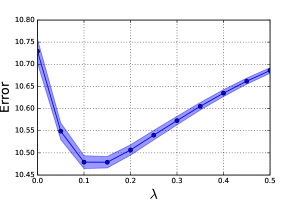
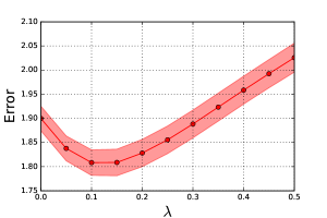
Figure 1: Cross-validation errors of (left) the negative log-likelihood $\mathcal{W}\left(A\right)-\mathbb{E}_{\hat{\pi}}\left[\Phi_{A}\left(X,Y\right)\right]$ (right) the covariance mismatch $\|\mathbb{E}_{\pi^{A}}\left[XY^{\top}\right]-\mathbb{E}_{\hat{\pi}}\left[XY^{\top}\right]\|_{F}$ .

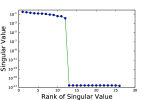
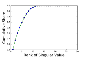
Figure 2: (Left) singular values (right) cumulative shares.

We use the low-rank optimal transport approach to estimate the affinity matrix $A$ when considering characteristics including the primary factors. Inspection of Figure 1 indicates that $\lambda=0.15$ gives slightly lower values of the CV errors of both $\mathcal{W}\left(A\right)-\mathbb{E}_{\hat{\pi}}\left[\Phi_{A}\left(X,Y\right)\right]$ and $\|\mathbb{E}_{\pi^{A}}\left[XY^{\top}\right]-\mathbb{E}_{\hat{\pi}}\left[XY^{\top}\right]\|_{F}$ than $\lambda=0.1$ does. Since $\lambda=0.15$ achieves this result with a lower rank of $A$, we use this value as the coefficient for the nuclear norm regularization. The left panel of Figure 2 reveals the rank of the affinity matrix is 12 hence indicating that only 12 relevant dimensions matter for matching affinities. Of those 12 relevant dimensions, the first three alone explain about 50% of the total matching affinity as indicated in the right panel of Figure 2.

The loadings of the first three dimensions, reported in Table 1, reveal several important results. First, as in Dupuy and Galichon (2014), we do find that the first relevant dimension loads principally on education, i.e. 0.85 for men and 0.83 for women respectively, whereas the second and third dimensions load principally on personality traits and attitude towards risk. However, using the primary factors rather than the global factors as in Dupuy and Galichon (2014), we find that although conscientiousness matters for both men and women, the underlying primary factors at play differ across gender. For women, the primary factor “easily hurt, offended,” belonging to the global factor conscientiousness, is the most important characteristic in the second dimension with a loading of 0.71. For men, the primary factor “easily hurt, offended” plays also an important role (loading of magnitude 0.42), but the primary factor “disciplined,” also belonging to the global factor conscientiousness, is the most important one with a loading of 0.52. These results clearly illustrates that although conscientiousness matters, not all of its primary constituents do and different aspects matter differently for men and women.

A similar type of results holds for the third dimension, which loads on some but not all of the items measuring attitude towards risk. However, this dimension also loads on other variables such as height, BMI and subjective health, making its interpretation more difficult.

4.2 Castes in India

The second application of our method is on data compiled by Banerjee et al. (2013). These data were collected based on interviews of Hindus families that placed a matrimonial ad in the major Bengali newspaper in India, between October 2002 and March 2003. A year after, 289 brides and grooms that had gotten married or engaged were interviewed a second time, resulting in, as labeled in Banerjee et al. (2013), the “matches” data. We use the sample of 284 couples for which information about the caste of both spouses is available. Based on this information, we create 8 dummy variables, one for each of the 8 main Hindus castes in India. In addition, the data contains information about the height, education, family origin (from west Bengal or not), the number of older (younger) brothers, the number of older (younger) sisters, income and per capita consumption of each spouse. To avoid deleting too many observations because of missing information on height and per capita consumption we proceeded as follows. For each of these variables, we replaced missing values by the sample mean and created a dummy variable indicating missing. Both, the imputed variable and the missing indicator were included into the set of characteristics considered in the analysis. Our working data set contains a sample of 284 couples with 19 characteristics observed for each spouse.

In this application, the analyst is therefore confronted with the problem of estimating an affinity matrix $A$ of size $19\times 19=361$ using a sample of $284$ couples. The ratio of 1.27 parameters per observation prevents the use of standard techniques unless one constructs combinations of the characteristics of spouses to reduce the size of the affinity matrix. A possibility to reduce the dimensionality of the model would be to group castes into larger classes. Since castes are organized hierarchically, the analyst could for instance define a threshold, grouping castes ranked below the threshold into one class and the others into a second class. The associated affinity matrix would have size $12\times 12$, resulting in $144$ parameters to be estimated with 284 couples, that is a ratio of roughly 1 parameter for 2 observations. However, this aggregation of castes into larger classes would impose restrictions on the role of castes in matching affinity. The chosen aggregation implies indeed that a man of say caste 1 has the same affinity for a woman of any caste within the same class. Given the rarity of inter-caste marriages and the evidence of same-caste preferences documented in Banerjee et al. (2013), this assumption does not seem to be justified. As an alternative, the low-rank optimal transport method introduced in this paper allows one to perform the estimation of the affinity matrix while selecting only the relevant combinations of characteristics that matter for the matching affinities.

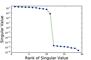
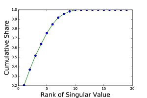
Figure 4: (Left) singular values (right) cumulative shares.

Figure 3 indicates that $\lambda=0.2$ gives slightly lower values of the CV errors of both $\mathcal{W}\left(A\right)-\mathbb{E}_{\hat{\pi}}\left[\Phi_{A}\left(X,Y\right)\right]$ and $\|\mathbb{E}_{\pi^{A}}\left[XY^{\top}\right]-\mathbb{E}_{\hat{\pi}}\left[XY^{\top}\right]\|_{F}$ than $\lambda=0.1$ or $\lambda=0.3$. We therefore select $\lambda=0.2$ for the analysis. The resulting affinity matrix has rank 10 as indicated in Figure 4 such that out of 19 possible dimensions of interaction only 10 are relevant. The first three dimensions together account for about 50% of the total matching affinity as shown in Figure 4.

Inspection of the loadings of the first three dimensions, reported in Table 2, clearly reveals the importance of castes in matching affinities. The first 3 dimensions on both sides have indeed large loadings on castes dummies. In the first dimension for instance, the dummy variable for being of the “Brahmin” caste has by far the largest loading, i.e. approximately 0.80, for both men and women. There is therefore a considerable loss in matching affinity for someone of the “Brahmin” caste to marry outside of his/her caste. Although less pronounced, we also find evidence for same-caste affinity for the “Kayastha,” “Baisya,” and “Sagdope” castes, as indicated by the relatively large loadings with same sign for men and women on the second dimension (for all three castes) and on the third (for the latter). These results tend to corroborate Banerjee et al. (2013)’s finding of same-caste marriage preferences. However, our results also reveal two important new findings. First, the “Baisya” and “Sagdope” castes both have positive loadings on the second dimension, which suggests a significant inter-caste matching affinity between spouses of these two castes. Second, in contrast, the “Kayastha” caste has a negative loading on the second dimension for both men and women. This indicates a negative (repulsive) matching affinity between men and women of the “Baisya” and “Sagdope” on the one hand and men and women of the “Kayastha” on the other hand.

Interestingly, education does not seem to play as an important role as in the previous application. However, as noted in Banerjee et al. (2013), this is probably due to the fact that the sample is representative, not of the whole population but rather of the Bengali middle-class that exhibits little variation in educational achievement: 85 percent of men and women in the sample have indeed at least a bachelor’s degree.

5 Conclusion and Future Research

In this paper, we have demonstrated the effectiveness of rank-constrained estimation techniques when solving inverse optimal transport problems. Inverse optimal transport problems are often faced with large dimensionality of the data sets; hence it is crucial to develop dimensionality reduction techniques. We plan to investigate further applications of this methodology, including explaining the intensity of mercantile exchanges between countries by the similarities in their characteristics, predicting stable matches in online dating platforms, or understanding the determinants of workers’ productivity on the labor market. We also plan to consider an extension of the present methodology to nonbipartite networks, which will allow to estimate the transport costs in minimum cost flow problems, with applications to analyzing urban transportation demand, as well as link formation in social networks.

Singular value
Singular vector
Oriented toward people
Quick thinker
Not easily worried
Stubborn, persistent
Vivid, vivacious
Meticulous
Dominant
Easily hurt, offended
Suspicious
Dreamer
Diplomatic, tactful
Doubts about myself
Open to changes
Independent, self-reliant
Disciplined
Irritable, quick tempered
Ready to take risk for high possible returns
Investments in shares are too risky
Ready to borrow money for risky investment
Want to be certain my investments are safe
Should take greater financial risks
Ready to risk losing money to gain money
Educational level
Height
BMI
Subjective health

$s_{1}=0.39$
$U_{1}$	$V_{1}$
-0.07	-0.04
0.08	-0.01
-0.10	0.00
0.06	0.03
0.00	0.02
-0.12	-0.05
0.05	0.06
-0.06	-0.03
0.08	0.01
-0.04	0.02
-0.06	0.07
0.06	0.13
0.10	0.03
-0.10	-0.11
0.01	0.01
0.00	-0.16
0.17	0.24
-0.31	-0.29
0.12	0.13
0.01	0.05
-0.06	-0.07
0.10	0.09
0.85	0.83
0.06	0.08
-0.20	-0.24
-0.01	0.01

$s_{2}=0.32$
$U_{2}$	$V_{2}$
-0.08	0.19
0.25	-0.12
0.29	0.11
0.11	0.14
0.04	0.19
-0.01	0.04
-0.09	-0.21
0.42	0.71
0.16	0.14
-0.08	0.23
0.07	-0.10
-0.31	-0.35
0.12	0.04
0.31	0.04
0.52	0.17
0.08	-0.17
-0.02	-0.07
0.05	-0.07
-0.16	-0.03
-0.12	0.02
-0.03	-0.05
0.06	-0.02
0.12	0.12
0.12	0.01
0.17	0.18
-0.15	-0.06

$s_{3}=0.24$
$U_{3}$	$V_{3}$
0.04	-0.08
-0.04	0.05
0.08	-0.07
-0.11	0.02
-0.23	0.11
0.16	0.17
0.00	0.08
0.02	-0.02
0.11	0.04
0.00	0.04
0.00	-0.03
0.17	0.09
-0.22	0.05
0.01	-0.09
0.01	-0.11
-0.02	-0.03
0.27	0.29
0.48	0.53
-0.17	-0.08
0.42	0.24
-0.11	-0.18
-0.38	-0.48
0.27	0.21
-0.12	-0.25
0.16	0.29
-0.21	-0.17

Table 1: Loadings of the top three relevant dimensions of matching affinities, Dutch couples.

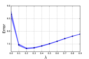
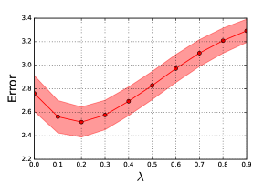
Figure 3: Cross-validation errors of (left) the negative log-likelihood $\mathcal{W}\left(A\right)-\mathbb{E}_{\hat{\pi}}\left[\Phi_{A}\left(X,Y\right)\right]$ (right) the covariance mismatch $\|\mathbb{E}_{\pi^{A}}\left[XY^{\top}\right]-\mathbb{E}_{\hat{\pi}}\left[XY^{\top}\right]\|_{F}$ .

Singular value
Singular vector
Height
Height missing
Educational level
Family from west Bengal
Number of older brothers
Number of younger brothers
Number of older sisters
Number of younger sisters
Income
Per capita consumption
Per capita consumption missing
Castes: 1 Brahmin
2 Baidya
3 Kshatriya
4 Kayastha
5 Baisya
6 Sagdope
7 Others
8 Scheduled castes

$s_{1}=0.53$
$U_{1}$	$V_{1}$
-0.22	-0.13
-0.02	0.27
0.09	0.01
0.12	0.13
0.08	-0.05
0.03	-0.03
-0.09	-0.08
-0.07	0.04
-0.11	0.06
0.02	-0.01
0.06	-0.04
0.80	0.79
-0.10	-0.03
-0.03	0.05
-0.30	-0.38
-0.34	-0.22
-0.06	-0.09
-0.13	-0.10
-0.10	-0.20

$s_{2}=0.43$
$U_{2}$	$V_{2}$
-0.05	0.13
-0.01	0.12
0.26	0.30
0.16	0.32
-0.06	-0.17
-0.01	-0.16
-0.06	0.13
-0.19	-0.09
0.24	-0.02
0.06	0.13
-0.06	0.22
-0.07	-0.15
-0.13	0.01
-0.05	0.10
-0.50	-0.41
0.40	0.39
0.57	0.48
-0.19	-0.23
0.06	-0.06

$s_{3}=0.38$
$U_{3}$	$V_{3}$
-0.21	-0.20
0.07	0.00
-0.27	-0.08
-0.37	-0.42
0.08	-0.08
0.03	0.18
0.05	0.10
0.17	-0.01
-0.21	-0.17
-0.25	-0.03
0.00	-0.10
0.12	0.09
-0.34	-0.37
-0.11	-0.05
-0.28	-0.34
0.51	0.57
-0.25	-0.20
0.15	0.11
0.21	0.22

Table 2: Loadings of the top three relevant dimensions of matching affinities, Indian couples.

References

- del Barrio, E., Giné, E., and Matrán, C. (1999). Central limit theorems for the Wasserstein distance between the empirical and the true distributions. Annals of Probability, 1009–1071.
- Banerjee, A., Duflo, E., Ghatak, M., and Lafortune, J. (2013). Marry for what? Caste and mate selection in modern India. American Economic Journal: Microeconomics, 5(2), 33–72.
- Becker, G. S. (1973). A theory of marriage: Part I. The Journal of Political Economy, 813–846.
- Benamou, J. D., Carlier, G., Cuturi, M., Nenna, L., and Peyré, G. (2015). Iterative Bregman projections for regularized transportation problems. SIAM Journal on Scientific Computing, 37(2), A1111–A1138.
- Burkard, R. E., Dell’Amico, M., and Martello, S. (2009). Assignment Problems, Revised Reprint. SIAM.
- Cattell, R. B., Cattell, A. K., and Cattell, H. E. P. (1993). 16PF fifth edition questionnaire. Champaign, IL: Institute for Personality and Ability Testing.
- Chiappori, P. A., Oreffice, S., and Quintana-Domeque, C. (2012). Fatter attraction: anthropometric and socioeconomic matching on the marriage market. Journal of Political Economy, 120(4), 659–695.
- Chiappori, P. A., Salanié, B., and Weiss, Y. (2016). Assortative matching on the marriage market: a structural investigation. American Economic Review, forthcoming.
- Donkers, B. and van Soest, A. (1999), Subjective measures of household preferences and financial decisions. Journal of Economic Psychology, 20(6), 613–642.
- Dupuy, A. and Galichon, A. (2014). Personality traits and the marriage market. Journal of Political Economy, 122(6), 1271–1319.
- Dupuy, A. and Galichon, A. (2015). Canonical correlation and assortative matching: A remark. Annals of Economics and Statistics, (119-120), 375–383.
- Fazel, M. (2002). Matrix rank minimization with applications (Doctoral dissertation, Stanford University).
- Fox, J. T. (2010). Identification in matching games. Quantitative Economics, 1(2), 203–254.
- Galichon, A. (2016). Optimal Transport Methods in Economics. Princeton University Press.
- Galichon, A. and Salanié, B. (2015). Cupid’s invisible hand: Social surplus and identification in matching models. Available at SSRN 1804623.
- Gautier, P. A., Svarer, M., and Teulings, C. N. (2010). Marriage and the city: Search frictions and sorting of singles. Journal of Urban Economics, 67(2), 206–218.
- Jepsen, L. K. (2005). The relationship between wife’s education and husband’s earnings: Evidence from 1960 to 2000. Review of Economics of the Household, 3(2), 197–214.
- Kalmijn, M. (1998). Intermarriage and homogamy: Causes, patterns, trends. Annual Review of Sociology, 395–421.
- Lam, D. and Schoeni, R. F. (1993). Effects of family background on earnings and returns to schooling: evidence from Brazil. Journal of Political Economy, 710–740.
- Lam, D. and Schoeni, R. F. (1994). Family ties and labor markets in the United States and Brazil. Journal of Human Resources, 1235–1258.
- Recht, B., Fazel, M., and Parrilo, P. A. (2010). Guaranteed minimum-rank solutions of linear matrix equations via nuclear norm minimization. SIAM Review, 52(3), 471–501.
- Shapley, L. S. and Shubik, M. (1971). The assignment game I: The core. International Journal of Game Theory, 1(1), 111–130.
- Suen, W. and Lui, H. K. (1999). A direct test of the efficient marriage market hypothesis. Economic Inquiry, 37(1), 29–46.
- Terviö, M. (2003). Studies of Talent Markets (Doctoral dissertation, MIT).
- Toh, K. C. and Yun, S. (2010). An accelerated proximal gradient algorithm for nuclear norm regularized linear least squares problems. Pacific Journal of Optimization, 6(615–640), 15.
- Villani, C. (2003). Topics in optimal transportation (No. 58). American Mathematical Society.
- Villani, C. (2008). Optimal transport: old and new (Vol. 338). Springer Science & Business Media.
- Watson, G. A. (1992). Characterization of the subdifferential of some matrix norms. Linear algebra and its applications, 170, 33–45.