Duality and topology

Abstract

Mappings between models may be obtained by unitary transformations with preservation of the spectra but in general a change in the states. Non-canonical transformations in general also change the statistics of the operators involved. In these cases one may expect a change of topological properties as a consequence of the mapping. Here we consider some dualities resulting from mappings, by systematically using a Majorana fermion representation of spin and fermionic problems. We focus on the change of topological invariants that results from unitary transformations taking as examples the mapping between a spin system and a topological superconductor, and between different fermionic systems.

1 Introduction

Many-body interacting systems are problems that are hard to solve, often requiring non-perturbative approaches to properly describe their cooperative phenomena. In general the complexity of the problem may be reduced identifying the dominant modes that govern the behavior of the system, particularly when a low-energy description is enough. Also, many authors have considered various transformations between variables or operators (depending if the system is classical or quantum, respectively) to obtain a good description of the system behavior and, in some cases, exactly solve the problem.

Depending on the problem, transformations from one set of operators to another may involve canonical transformations [1], preserving the statistics, or non-canonical transformations, where the statistics is altered. Typical examples are bosonization of a fermionic problem or, reversely, fermionization. Also, often it is convenient to transform between spin and fermionic problems. Some transformations are exact [2, 3, 4] but in some cases there is an enlargement of the Hilbert space, and a projection to the physical subspace is required [5, 6, 7, 8, 9, 10, 11, 12]. The simplest cases involve local transformations from one set of operators to another, but non-local transformations are also convenient in some cases. Also, some transformations have an intrinsic non-linear character [1]. A familiar example are the bilinear representations of spin operators in terms of bosonic or fermionic operators [13]. Since the transformation between the two sets of operators is bilinear, it naturally provides a way for a non-canonical transformation with consequent change of statistics. In some cases it has been shown that performing a mapping between spin and fermionic systems it is possible to reduce an apparent interacting term into a free problem, with the consequent exact solution. An example is provided by a X-Y chain which may be reduced to a problem of free (in the sense of quadratic) problem of spinless fermions [14, 15], the so-called fermionic Kitaev model [16]. This example illustrates a problem of statistical transmutation of an original problem of spins into a problem of fermions. This is well known to be achieved applying a Jordan-Wigner transformation [17] which traditionally is understood as a transformation between operators defined such that their commutation relations are satisfied. Other non-canonical transformations include the Schrieffer-Wolff transformation [18] between the Anderson model and the Kondo model and bosonization between fermions and a bosonic field [19]. The Jordan-Wigner transformation that leads to the Kitaev model is reviewed in Appendix A.

In this work we will focus on fermionic and spin-$1/2$ systems. Among the many representations for spin systems one is particularly convenient since it allows an exact preservation of the commutation relations of the spin operators [20, 21, 22]. There is some enlargement of the Hilbert space but it just leads to a multiplying factor in the partition function of the system [23, 24, 25]. Specifically, the spin operators may be represented by a bilinear representation in terms of three Majorana operators. The spin-$1/2$ representation in terms of Majoranas has been applied in several contexts [21, 22, 25, 24, 26, 27]. Majorana operators may also be used to represent a fermionic operator in a simple way. A fermionic operator may be understood as containing real and imaginary parts if these are chosen as hermitian operators, which is the characteristic property of a Majorana fermion. It is therefore convenient to look for transformations between spin and fermionic operators using a language of transformation operators in terms of Majorana fermions. Looking for general transformations using Majorana operators, it is possible to consider different choices of representations which enable both canonical and non-canonical transformations. In addition, it has been proposed that they provide a convenient way to understand the general properties of transformations between operators [28, 29].

The interest in Majorana fermions has recently been revived due to their possible relevance in quantum computation problems and have been proposed to be observed in the context of topological superconductors [30]. Even though appropriate materials are difficult to find in nature, several engineered possibilities have been proposed such as semiconductor wires with strong spin-orbit coupling placed on top of a conventional superconductor and in the presence of a Zeeman field [31], or magnetic impurities on top of a conventional superconductor [32]. In these systems the Majorana modes are associated with edge modes at the border between a topologically non-trivial system and a trivial system.

The transformation between sets of operators or variables leads to an equivalent problem whose Hamiltonian is expressed in terms of other physical quantities. In some loose sense we may think of a transformation as a relation between dual Hamiltonians. Dualities appear in physics in various contexts from dualities in classical electromagnetism (between electric and magnetic fields at the level of Maxwell’s equations), dualities in statistical physics problems (such as the Kramers-Wannier identities [33] that relate the partition function of the system in the low and high temperature limits) and dual lattices (by establishing a relation between variables or operators defined at the corners or links of some lattice problem).

As pointed out recently [34] the duality transformations do not need to relate strong and weak coupling regimes (although they are particularly useful when this occurs), and usually are non-local relationships involving often some kind of extended strings of operators. Intrinsic to the idea of duality and the search of an alternative set of operators to describe the properties of some Hamiltonian, is the equivalence between the two descriptions. An expected minimal requirement is that the spectrum of the Hamiltonian is preserved. An obvious way to achieve this is to consider unitary transformations since the spectrum is preserved. However, in general, the states are not preserved even though the relation between them is determined by the choice of the unitary operator. As a consequence of the change of states it has been pointed out that, in general, level degeneracy changes and therefore the correspondence between the two Hamiltonians is not complete.

It has also been pointed out recently that the usual non-local character of the duality transformation suggests that the use of bond operators may be more convenient than local relations. In reference [34] several transformations have been considered and the standard example of a Jordan-Wigner transformation between a spin-$1/2$ problem and a spinless fermion non-interacting Hamiltonian has been derived with the bond-duality approach. In the case of nearest-neighbor couplings this transformation has been known for a long time to fully diagonalize the Hamiltonian, since in the fermionic language is non-interacting. However, it is also known that the Jordan-Wigner transformation may be seen as the result of a local unitary transformation [24] (understood as a product of local transformations across all lattice sites). In this work we will follow a similar procedure and therefore consider a less stringent definition of duality (see also, for instance [35]).

The mapping between the $XY$ spin model in a transverse field and the Kitaev superconducting model [16] reveals another interesting result. While the original spin problem is topologically trivial, the resulting transformed Hamiltonian has topological regimes. Therefore, as a consequence of the exact transformation between the two problems, it appears that the topological properties have changed. On the other hand, it has been shown recently that it is possible to transform topological insulators to topological superconductors [36]. In this case this is a canonical transformation. It was shown that topological phases are matched to topological phases and trivial phases to trivial phases. This suggests that a non-canonical transformation may be required to change topology.

Topological systems appear in various contexts. To name a few, among those that have received recently considerable attention are the topological insulators and topological superconductors [37, 38, 39] due to their robust edge states with possible applications in dissipation free transport and quantum computation. Other well-known topological systems are some spin chains. An example of phases with topological origin are the gapped Haldane phases [40] of odd integer spin chains that find an exact realization in the gapped AKLT phases [41], where non-local string order has been found. This hidden order is the result of a hidden order symmetry [42, 43] and may be understood as the result of a non-local unitary transformation [44, 45]. One may search for correlation functions in a topological system that are related via duality with the order parameters in the trivial but ordered dual system [46, 47, 48]. True topologically ordered systems display long-range topological order that may not be eliminated by any local transformation [49, 50].

The work is organized as follows: In section 2 we consider the action of general unitary transformations on fermion and spin operators, expressed in terms of Majorana fermion operators. In section 3 we consider mappings between spin and fermionic systems using a non-canonical unitary transformation that allows a mapping between a nearest-neighbor spin problem and a system of free spinless fermions. In section 4 we consider topological invariants for different representations of the fermionic operators of Kitaev’s model. In section 5 we focus on the transformation between a spin problem and a corresponding fermionic problem and discuss the role of boundary conditions on topological properties. We conclude with section 6.

2 Unitary transformations of fermion and spin operators

2.1 Fermion, Majorana and spin operators

In general, a fermion operator at site $j$ may be written in terms of two hermitian operators, $\gamma_{1},\gamma_{2}$, in the following way

$$c_{j,\sigma} = \frac{1}{2}\left(\gamma_{j,\sigma,1}+i\gamma_{j,\sigma,2}\right)$$

$$c_{j,\sigma}^{\dagger} = \frac{1}{2}\left(\gamma_{j,\sigma,1}-i\gamma_{j,\sigma,2}\right)$$ (1)

The index $\sigma$ represents internal degrees of freedom of the fermionic operator, such as spin and/or sublattice index. In general, the $\gamma$ operators we will consider are hermitian and satisfy a Clifford algebra $\{\gamma_{m,i},\gamma_{n,j}\}=2\delta_{ij}\delta_{mn}I$, where $m,n=j,\sigma$, and $I$ is the identity. We use the normalization $\gamma_{i}^{2}=1$ and $i=1,2,3$.

Majoranas also allow a representation of spin-$1/2$ problems. One needs three Majorana operators to represent local spin operators as

$$S_{x}=-(i/2)\gamma_{2}\gamma_{3};\hskip 28.45274ptS_{y}=-(i/2)\gamma_{3}\gamma_{1};\hskip 28.45274ptS_{z}=-(i/2)\gamma_{1}\gamma_{2}.$$ (2)

It is convenient to define the operators $\mathscr{S}_{i}=\frac{-i}{2}\epsilon_{ijk}\gamma_{j}\gamma_{k}$, differing in normalization from the standard spin operators $\vec{S}=\frac{1}{2}\vec{\mathscr{S}}$, and the operator $I_{3}=-i\gamma_{1}\gamma_{2}\gamma_{3}=\frac{-i}{6}\epsilon_{ijk}\gamma_{i}\gamma_{j}\gamma_{k}$.

With the definition of these operators, the multiplication rule of the Majorana operators becomes

$$\gamma_{i}\gamma_{j}=\delta_{ij}I+i\epsilon_{ijk}\mathscr{S}_{k}$$ (3)

from which it follows that $\vec{\gamma}^{2}=3I$. The multiplication rules of the Majorana and spin operators are given by

$$\gamma_{i}\mathscr{S}_{j} = \delta_{ij}I_{3}+i\epsilon_{ijk}\gamma_{k}$$ (4)

$$\mathscr{S}_{i}\gamma_{j} = \delta_{ij}I_{3}+i\epsilon_{ijk}\gamma_{k}$$ (5)

and

$$\mathscr{S}_{i}\mathscr{S}_{j}=\delta_{ij}I+i\epsilon_{ijk}\mathscr{S}_{k}$$ (6)

together with $I_{3}^{2}=I$, $I_{3}\gamma_{i}=\gamma_{i}I_{3}=\mathscr{S}_{i}$, and $I_{3}\mathscr{S}_{i}=\mathscr{S}_{i}I_{3}=\gamma_{i}$. One also has $\vec{\mathscr{S}}^{2}=3I$ and $\vec{\gamma}\cdot\vec{\mathscr{S}}=\vec{\mathscr{S}}\cdot\vec{\gamma}=3I_{3}$. These equations can be summarized as that the operators $\gamma_{i}$ and $\mathscr{S}_{i}$ follow multiplication rules similar to the Pauli matrices, but paying attention to their nature, i.e. being odd or even in the Majorana operators, and that the multiplication by $I_{3}$ transforms $\gamma_{i}$ into $\mathscr{S}_{i}$ and vice versa.

2.2 Enlargement of Hilbert space

An interesting question when representing fermions and spins using Clifford algebras is the enlargement of the number of states and the resulting degeneracy of the states. In the case of the treatment of fermion systems there is no enlargement of the number of states. With the fermionic operators $c=\frac{1}{2}\left(\gamma_{1}+i\gamma_{2}\right),c^{\dagger}=\frac{1}{2}\left(\gamma_{1}-i\gamma_{2}\right)$ one can define the Majorana operators $\gamma_{1}=c^{\dagger}+c$ and $\gamma_{2}=i\left(c^{\dagger}-c\right)$. The operator $\mathscr{S}_{3}=-i\gamma_{1}\gamma_{2}=\left(2c^{\dagger}c-1\right)$ anticommutes with both $\gamma_{1}$ and $\gamma_{2}$, but is not independent from them, and there is no enlargement of the number of states, which continues to be $2$. However, when one considers bilinear representations of spin operators in terms of Clifford operators an enlargement of the number of states occurs, resulting from the $\mathbb{Z}_{2}$ symmetry implied by the bilinear representation.

In the case of a single spin operator, there is a duplication of the number of states, with $4$ states instead of $2$. The easier way to understand this is to introduce an extra Clifford operator to pair with the third to give a second pair of creation and destruction operators. Applying this procedure to a set of $N$ spins $\frac{1}{2}$ one has then $2^{2N}$ states instead of $2^{N}$. In general, if one has $N$ spins $\frac{1}{2}$, the number of states is $2^{N}$. Introducing three Clifford operators for each spin, one has $3N$ Majorana operators. If the number of sites $N$ is even, we can associate them in pairs obtaining $\frac{3N}{2}$ pairs of fermion operators, and the number of states will be $2^{\frac{3N}{2}}$. If the number of states is odd, one introduces then an extra Clifford operator and the number of states is $2^{\frac{3N+1}{2}}$.

As is well known, the complex Clifford algebras have the algebraic isomorphisms $Cl(n)=\mathbb{C}(2^{\frac{n}{2}})$ if $n$ is even, and $Cl(n)=\mathbb{C}(2^{\frac{n-1}{2}})\oplus\mathbb{C}(2^{\frac{n-1}{2}})$ if $n$ is odd [51, 52]. If $n$ is even, the algebra is central simple, but if $n$ is odd, besides the identity, the center also includes the product of all the Clifford operators, and one can define a projection into an even and an odd algebra under the normalized product of all the Clifford operators, similarly to the results shown in Appendix B for $I_{\pm}=\frac{1}{2}(I\pm I_{3})$, $\Sigma^{\pm}_{i}=\frac{1}{2}(\mathscr{S}_{i}\pm\gamma_{i})$ and $I_{3}$.

The case of two spins and of its degeneracy has been discussed in the literature [24, 25], showing that for the Heisenberg interaction, the singlet and triplet states become both doubly represented, and that, as a result, the partition function is simply multiplied by this multiplicity factor. In [24], the case of an electron with spin is also discussed at length, showing that the usual spin electron operator, associated to the spin degree of freedom, and the Nambu pseudospin operator, associated to the charge degree of freedom, are orthogonal, with their sum providing a doubly representation of $SU(2)$. Again, the partition function is simply multiplied by a multiplicity factor, even in the case of many electrons with a spin-spin interaction between the sum of the spin and pseudospin of each electron.

2.3 Action of unitary and hermitian transformations on local operators

Let us first consider general local transformations on the spin and Majorana operators of the type $U^{2}=I$, therefore unitary transformations that are also hermitian operators. Let us look for solutions of the type

$$U=zI+\omega I_{3}+\vec{x}\cdot\vec{\gamma}+\vec{y}\cdot\vec{\mathscr{S}}$$ (7)

Here $I_{3}=i\gamma_{1}\gamma_{2}\gamma_{3}$, $\vec{\mathscr{S}}=2\vec{S}$ and $z,\omega,\vec{x},\vec{y}$ are real numbers. These imply that $U$ is unitary. The solutions of $U^{2}=I$ may be organized into the following classes:

• (i) $U=I$

• (ii) $U=I_{3}$

• (iii) $U=\frac{1}{2}\left(I+I_{3}+\vec{n}_{-}\cdot\frac{1}{2}\left(\vec{\mathscr{S}}-\vec{\gamma}\right)\right)$, with $|\vec{n}_{-}|=1$

• (iv) $U=\pm\frac{1}{2}\left(I-I_{3}+\vec{n}_{+}\cdot\frac{1}{2}\left(\vec{\mathscr{S}}+\vec{\gamma}\right)\right)$, with $|\vec{n}_{+}|=1$

• (v) $U=\cos\frac{\theta}{2}\vec{n}_{1}\cdot\vec{\gamma}+\sin\frac{\theta}{2}\vec{n}_{2}\cdot\vec{\mathscr{S}}$, with $|\vec{n}_{1}|=|\vec{n}_{2}|=1$ and $\vec{n}_{1}\cdot\vec{n}_{2}=0$.

Both in classes (i) and (ii) we find that acting on operators on a given site we get $U\vec{\gamma}U^{\dagger}=\vec{\gamma}$ and $U\vec{\mathscr{S}}U^{\dagger}=\vec{\mathscr{S}}$. In the case of class (iii) we get

$$U\frac{1}{2}\left(\vec{\mathscr{S}}-\vec{\gamma}\right)U^{\dagger} = 2\vec{n}\left(\vec{n}\cdot\frac{1}{2}(\vec{\mathscr{S}}-\vec{\gamma})\right)-\frac{1}{2}\left(\vec{\mathscr{S}}-\vec{\gamma}\right)$$

$$U\vec{\gamma} U^{\dagger} = \vec{\mathscr{S}}-\vec{n}\left(\vec{n}\cdot(\vec{\mathscr{S}}-\vec{\gamma})\right)$$

$$U\vec{\mathscr{S}} U^{\dagger} = \vec{\gamma}+\vec{n}\left(\vec{n}\cdot(\vec{\mathscr{S}}-\vec{\gamma})\right)$$ (8)

In the case of class (iv) we get that

$$U\vec{\gamma} U^{\dagger} = -\vec{\mathscr{S}}+\vec{n}\left(\vec{n}\cdot(\vec{\mathscr{S}}+\vec{\gamma})\right)$$

$$U\vec{\mathscr{S}} U^{\dagger} = -\vec{\gamma}+\vec{n}\left(\vec{n}\cdot(\vec{\mathscr{S}}+\vec{\gamma})\right)$$ (9)

Finally, in the case of class (v) we get that

$$U\vec{\gamma} U^{\dagger} = -\vec{\gamma}+2\left[(\cos\frac{\theta}{2})^{2}\vec{n}_{1}\left(\vec{n}_{1}\cdot\vec{\gamma}\right)\right.$$

$$+ \left.(\sin\frac{\theta}{2})^{2}\vec{n}_{2}\left(\vec{n}_{2}\cdot\vec{\gamma}\right)\right.$$

$$+ \left.\sin\frac{\theta}{2}\cos\frac{\theta}{2}\left(\vec{n}_{1}(\vec{n}_{2}\cdot\vec{\gamma})+\vec{n}_{2}(\vec{n}_{1}\cdot\vec{\gamma})\right)\right]$$

$$U\vec{\mathscr{S}} U^{\dagger} = -\vec{\mathscr{S}}+2\left[(\cos\frac{\theta}{2})^{2}\vec{n}_{1}\left(\vec{n}_{1}\cdot\vec{\mathscr{S}}\right)\right.$$ (10)

$$+ \left.(\sin\frac{\theta}{2})^{2}\vec{n}_{2}\left(\vec{n}_{2}\cdot\vec{\mathscr{S}}\right)\right.$$

$$+ \left.\sin\frac{\theta}{2}\cos\frac{\theta}{2}\left(\vec{n}_{1}(\vec{n}_{2}\cdot\vec{\gamma})+\vec{n}_{2}(\vec{n}_{1}\cdot\vec{\gamma})\right)\right]$$

2.4 General unitary operations

Let us now consider local transformations that are unitary but not hermitian. Some possible examples are illustrated next.

(a) $U=\frac{1}{\sqrt{2}}\left(1+i\vec{n}\cdot\vec{\mathscr{S}}\right)$, with $|\vec{n}|=1$. The action of this operator leads to

$$U\vec{\mathscr{S}}U^{\dagger} = \vec{n}\left(\vec{n}\cdot\vec{\mathscr{S}}\right)+\vec{n}\times\vec{\mathscr{S}}$$

$$U\vec{\gamma}U^{\dagger} = \vec{n}\left(\vec{n}\cdot\vec{\gamma}\right)+\vec{n}\times\vec{\gamma}$$ (11)

The action of this unitary operator does not change the nature of the operators and therefore is an example of a canonical transformation.

(b) $U=\frac{1}{\sqrt{2}}\left(1+i\vec{n}\cdot\vec{\gamma}\right)$, with $|\vec{n}|=1$. The action of this operator leads to

$$U\vec{\gamma}U^{\dagger} = \vec{n}\left(\vec{n}\cdot\vec{\gamma}\right)+\vec{n}\times\vec{\mathscr{S}}$$

$$U\vec{\mathscr{S}}U^{\dagger} = \vec{n}\left(\vec{n}\cdot\vec{\mathscr{S}}\right)+\vec{n}\times\vec{\gamma}$$ (12)

mixing the nature of the operators and therefore is an example of a non-canonical transformation.

(c) $U=\frac{1}{\sqrt{2}}\left(I_{3}+i\vec{n}\cdot\vec{\gamma}\right)$, with $|\vec{n}|=1$ and $I_{3}=-i\gamma_{1}\gamma_{2}\gamma_{3}$. The action of this operator leads to a set of canonical transformations

$$U\vec{\gamma}U^{\dagger} = \vec{n}\left(\vec{n}\cdot\vec{\gamma}\right)+\vec{n}\times\vec{\gamma}$$

$$U\vec{\mathscr{S}}U^{\dagger} = \vec{n}\left(\vec{n}\cdot\vec{\mathscr{S}}\right)+\vec{n}\times\vec{\mathscr{S}}$$ (13)

(d) $U=\cos\theta/2+i\sin\theta/2\vec{n}\cdot\vec{\gamma}$ leads to

$$U\vec{\gamma}U^{\dagger} = \vec{n}\left(\vec{n}\cdot\vec{\gamma}\right)+\cos\theta\left(\vec{\gamma}-\vec{n}\left(\vec{n}\cdot\vec{\gamma}\right)\right)$$

$$+ \sin\theta\left(\vec{n}\times\vec{\mathscr{S}}\right)$$

$$U\vec{\mathscr{S}}U^{\dagger} = \vec{n}\left(\vec{n}\cdot\vec{\mathscr{S}}\right)+\cos\theta\left(\vec{\mathscr{S}}-\vec{n}\left(\vec{n}\cdot\vec{\mathscr{S}}\right)\right)$$

$$+ \sin\theta\left(\vec{n}\times\vec{\gamma}\right)$$

which is also non-canonical since it mixes the two types of operators, Majoranas and spin operators.

Note that from

$$U=\frac{1}{2}\left[I+I_{3}-\vec{n}\cdot\left(\vec{\mathscr{S}}-\vec{\gamma}\right)\right]$$ (15)

choosing $\vec{n}=\vec{e}_{z}$ we get that

$$U = \frac{1}{2}\left[I+I_{3}+\gamma_{3}-\mathscr{S}_{3}\right]$$ (16)

$$= \frac{1}{2}\left[1-i\gamma_{1}\gamma_{2}\gamma_{3}+\gamma_{3}+i\gamma_{1}\gamma_{2}\right]=U_{z}$$

Also, note that

$$U_{z}\mathscr{S}_{z}U_{z}=\mathscr{S}_{z}\hskip 28.45274ptU_{z}\mathscr{S}_{x}U_{z}=\gamma_{1}\hskip 28.45274ptU_{z}\mathscr{S}_{y}U_{z}=\gamma_{2}$$ (17)

This class of transformations given by $\vec{n}=\vec{e}_{\alpha}$ leaves one of the spin operator components invariant, $U_{\alpha}\mathscr{S}_{\alpha}U_{\alpha}=\mathscr{S}_{\alpha}$ for $\alpha=x,y,z$ $(1,2,3)$. The transformation acts in the perpendicular plane.

e) Consider now the following unitary operator of class (v)

$$U_{v}=\cos\frac{\theta}{2}\vec{n}_{1}\cdot\vec{\gamma}+\sin\frac{\theta}{2}\vec{n}_{2}\cdot\vec{\mathscr{S}}=U_{v}^{\dagger}$$ (18)

with $\vec{n}_{1}\cdot\vec{n}_{2}=0$. Take for instance $\vec{n}_{1}=\vec{e}_{x},\vec{n}_{2}=\vec{e}_{y}$. Then

$$U_{v}=\cos\frac{\theta}{2}\gamma_{1}+\sin\frac{\theta}{2}\mathscr{S}_{2}=\cos\frac{\theta}{2}\gamma_{1}-i\sin\frac{\theta}{2}\gamma_{3}\gamma_{1}$$ (19)

The action of the operator on the spin components is

$$U_{v}\mathscr{S}_{x}U_{v} = \cos\theta\mathscr{S}_{1}+\sin\theta\gamma_{2}$$

$$U_{v}\mathscr{S}_{y}U_{v} = -\cos\theta\mathscr{S}_{2}+\sin\theta\gamma_{1}$$ (20)

Also, taking two sites $l$ and $j$

$$U_{v,l}\gamma_{\alpha,j}U_{v,l}=\left(-\cos\theta+i\sin\theta\gamma_{3,l}\right)\gamma_{\alpha,j}$$ (21)

with $\alpha=1,2,3$.

Having established several possible transformations between spin and fermionic operators one may now use them to construct exact mappings between different models. Our focus here will be on the transformation mentioned above between a spin model and its fermionic description and on the effect of different fermionic representations on topology.

3 Mapping between spins and fermions

3.1 Non-canonical unitary transformation

The Jordan-Wigner transformation may also be constructed (see appendix in Ref. [24]) introducing the local unitary transformation $U_{z}$. To simplify let us consider the XX model ($J_{x}=J_{y}=1$) or the fully anisotropic $X$ model ($J_{x}=1,J_{y}=0$) model

$$H_{X}=\frac{1}{4}\sum_{j}\left(S^{+}_{j}S^{-}_{j+1}+S^{-}_{j}S^{+}_{j+1}+S^{+}_{j}S^{+}_{j+1}+S^{-}_{j}S^{-}_{j+1}\right)$$ (22)

The spin operators may be represented by the Majorana operators as [20, 21] $S^{+}=\gamma_{3}\left(\gamma_{1}+i\gamma_{2}\right)/2$, $S^{-}=\left(\gamma_{1}-i\gamma_{2}\right)\gamma_{3}/2$. Define now usual fermionic operators (non-hermitian) as $g=\frac{1}{2}\left(\gamma_{1}-i\gamma_{2}\right)$, $g^{\dagger}=\frac{1}{2}\left(\gamma_{1}+i\gamma_{2}\right)$. We get that $\gamma_{1}=g+g^{\dagger}$ and $i\gamma_{2}=g^{\dagger}-g$. Therefore we may write the Hamiltonians as

$$H_{XX} = \frac{1}{2}\sum_{j}\left(g_{j}^{\dagger}g_{j+1}+g_{j}g_{j+1}^{\dagger}\right)\gamma_{3,j}\gamma_{3,j+1}$$

$$H_{X} = \frac{1}{4}\sum_{j}\left(g_{j}^{\dagger}g_{j+1}+g_{j}g_{j+1}^{\dagger}-g_{j}^{\dagger}g_{j+1}^{\dagger}-g_{j}g_{j+1}\right)\gamma_{3,j}\gamma_{3,j+1}$$ (23)

The Hamiltonian in terms of the Majorana and regular fermions is interacting, as evidenced by the quartic terms in the Hamiltonian. A possible way to diagonalize the Hamiltonian is to perform a unitary transformation that eliminates the $\gamma_{3}$ operators. This can be achieved using the local unitary and hermitian operator [24]

$$U_{z,j} = \left(1-g_{j}^{\dagger}g_{j}\right)+\gamma_{3,j}g_{j}^{\dagger}g_{j}$$ (24)

$$= \frac{1}{2}\left[1+i\gamma_{1,j}\gamma_{2,j}+\gamma_{3,j}-i\gamma_{1,j}\gamma_{2,j}\gamma_{3,j}\right]$$

Defining now an operator that is the product over all sites in the one-dimensional system

$$U_{z}=\prod_{j=1}^{N}U_{z,j}=U_{z,1}\cdots U_{z,N}$$ (25)

we get

$$U_{z}\gamma_{3,j}g_{j}^{\dagger}U_{z}^{\dagger}=\left(-1\right)^{\sum_{l=1}^{j-1}n_{l}}g_{j}^{\dagger}$$ (26)

and its hermitian conjugate. We see that this unitary transformation gives origin to the so-called strings associated with the occupation of states to the left of a given lattice site, $j$. This is like in the Jordan-Wigner transformation. Applying to the Hamiltonian

$$U_{z}H_{XX}U_{z}^{\dagger}=-\frac{1}{2}\sum_{j}\left[g_{j}^{\dagger}g_{j+1}+g_{j+1}^{\dagger}g_{j}\right]$$ (27)

Similarly [24]

$$U_{z}H_{X}U_{z}^{\dagger}=-\sum_{j}\left[g_{j}^{\dagger}g_{j+1}+g_{j+1}^{\dagger}g_{j}+g_{j}^{\dagger}g_{j+1}^{\dagger}+g_{j+1}g_{j}\right]$$ (28)

which is Kitaev’s model [16] for $t=1,\Delta=1$. In contrast to the original model which described interacting spins on a lattice, this model describes spinless fermions that may hopp on a lattice and have a nearest-neighbor $p$-type superconducting pairing, as shown by the appearance of creation and destruction pair operators. A magnetic field term is invariant (see Eq. (2)). We can also write

$$H_{X}=\frac{1}{4}\sum_{j}\gamma_{2,j}\gamma_{2,j+1}\gamma_{3,j}\gamma_{3,j+1}$$ (29)

This quartic Hamiltonian is transformed to a quadratic Hamiltonian by eliminating the $\gamma_{3}$ terms since the action of the unitary operator $U_{z,j}$ is of the form

$$U_{z,j}\gamma_{2,j}\gamma_{3,j}U_{z,j}^{\dagger}=i\gamma_{1,j}$$ (30)

can be seen as transforming a spin-like operator (bilinear in the Majoranas) into a Majorana operator. We may also see that $U_{z,j}\gamma_{1,j}\gamma_{3,j}U_{z,j}^{\dagger}=-i\gamma_{2,j}$. Noting now that

$$\left(\prod_{l=1}^{j-1}U_{z,l}\right)\gamma_{1,j}\left(\prod_{l=j-1}^{1}U_{z,l}^{\dagger}\right)=\gamma_{1,j}\prod_{l=1}^{j-1}\left[i\gamma_{1,l}\gamma_{2,l}\right]$$ (31)

we get

$$U_{z}H_{X}U_{z}^{\dagger}=\frac{i}{4}\sum_{j}\gamma_{2,j}\gamma_{1,j+1}.$$ (32)

which is a non-interacting fermionic problem.

3.2 Relation between fermionic states and spin states and order parameter correspondence

The mapping of Kitaev’s model to the spin system identifies $\Delta=t$ with $J_{y}=0$ (see Eq. (123). Consider therefore the $X$ chain in the ferromagnetic case $H_{X}=-\sum_{j}S_{x,j}S_{x,j+1}$. The groundstate is $|GS\rangle=|\sigma_{x}=1;\sigma_{x}=1;\cdots;\sigma_{x}=1;\cdots\rangle$ or $\sigma_{x}=-1$ at every site ($Z_{2}$ degeneracy). The solution for the antiferromagnetic model is presented in [14]. Recall that $\sigma_{x}=\mathscr{S}_{x}=-i\gamma_{2}\gamma_{3}$. Therefore the action of an operator at a given lattice site on the groundstate is $(-i)\gamma_{2}\gamma_{3}|GS\rangle=|GS\rangle$.

Define now new local fermionic operators in terms of the Majorana operators used to represent the spin operators as $f_{j}=\frac{1}{2}\left(\gamma_{2,j}+i\gamma_{3,j}\right)$ and $f_{j}^{\dagger}=\frac{1}{2}\left(\gamma_{2,j}-i\gamma_{3,j}\right)$. Similarly to previous results it is easy to see that $2f_{j}^{\dagger}f_{j}-1=i\gamma_{2,j}\gamma_{3,j}$. Therefore, $\mathscr{S}_{1,j}=-i\gamma_{2,j}\gamma_{3,j}=-\left(2f_{j}^{\dagger}f_{j}-1\right)$. Therefore we can identify $|\mathscr{S}_{x}=1\rangle=|0\rangle_{f}$, $|\mathscr{S}_{x}=-1\rangle=|1\rangle_{f}$. In other words the groundstate can be chosen as $|GS\rangle=|0;0;\cdots;0;\cdots\rangle_{f}$.

We can now see the influence of the $U_{z}$ operator previously defined on the groundstate. One possible way to see this is to consider that when acting on a state with $n_{f}=0$ the operator $-i\gamma_{2}\gamma_{3}=I$, acts as the identity, $I_{j}$. Acting with the unitary operator, $U_{z}$, and using that $g^{\dagger}=(\gamma_{1}+i\gamma_{2})/2$ and $i\gamma_{1}\gamma_{2}=1-2g^{\dagger}g$, we find that

$$U_{z}|0\rangle_{f} = \prod_{j=1}^{N}\frac{1}{2}\left[\gamma_{1}+i\gamma_{2}+\gamma_{1}\gamma_{3}-i\gamma_{2}\gamma_{3}\right]_{j}|0\rangle_{f}$$ (33)

$$= \prod_{j=1}^{N}\left[1+g^{\dagger}-g^{\dagger}g\right]_{j}|0\rangle_{f}$$

Using that $|\mathscr{S}_{x}=1\rangle\sim|\mathscr{S}_{z}=1\rangle+|\mathscr{S}_{z}=-1\rangle$ this implies that $|0\rangle_{f}\sim|0\rangle_{g}+|1\rangle_{g}$. So,

$$U_{z}|GS\rangle\sim\prod_{j=1}^{N}\left[1+g^{\dagger}\right]_{j}|0\rangle_{g}\sim|\psi^{+}_{0}\rangle$$ (34)

with $|\psi^{+}_{0}\rangle=|\psi^{0}_{even}\rangle+|\psi^{0}_{even}\rangle$, see Eq. 131. So, the states are proportional, as expected [53]. Using the unitary operator that transforms the spin Hamiltonian to the Kitaev spinless fermion model we also transform between the groundstates of the two models:

$$U_{z}|GS\rangle^{spins}\sim|GS\rangle^{Kitaev}_{g}\sim|GS\rangle_{d}$$ (35)

The operators $g$ and $f$ may be related by a unitary transformation that transforms $\mathscr{S}_{x}$ into $\mathscr{S}_{z}$. Choosing a local operator as $\bar{U}=\frac{1}{\sqrt{2}}\left(1-\gamma_{1}\gamma_{3}\right)$, we can show that $\bar{U}f^{\dagger}\bar{U}^{\dagger}=ig$. Its action on the spin operators may be determined and yields

$$\bar{U}\mathscr{S}_{x}\bar{U}^{\dagger}=\mathscr{S}_{z}\hskip 28.45274pt\bar{U}\mathscr{S}_{y}\bar{U}^{\dagger}=\mathscr{S}_{y}\hskip 28.45274pt\bar{U}\mathscr{S}_{z}\bar{U}^{\dagger}=-\mathscr{S}_{x}$$ (36)

Also,

$$\bar{U}\gamma_{1}\bar{U}^{\dagger}=\gamma_{3}\hskip 28.45274pt\bar{U}\gamma_{2}\bar{U}^{\dagger}=\gamma_{2}\hskip 28.45274pt\bar{U}\gamma_{3}\bar{U}^{\dagger}=-\gamma_{1}$$ (37)

The state $|0\rangle_{f}$ may be expanded as $|0\rangle_{f}=\alpha|0\rangle_{g}+\beta|1\rangle_{g}$. Acting with the creation operator $f^{\dagger}$ we may obtain that $|1\rangle_{f}=-i\left(\alpha|1\rangle_{g}-\beta|0\rangle_{g}\right)$. Imposing that $\langle 1|0\rangle_{f}=0$ we get $\beta^{*}\alpha=\alpha^{*}\beta$, and using that $\langle\sigma_{x}=1|\sigma_{z}|\sigma_{x}=1\rangle=0$ we obtain that $|\beta|^{2}=|\alpha|^{2}$. Using that $|0\rangle_{f}$ is normalized $|\alpha|^{2}+|\beta|^{2}=1$ we get that $\alpha=\beta=1/\sqrt{2}$.

At zero temperature one may consider the operator $\sigma_{x}=-i\gamma_{2}\gamma_{3}$ as the order parameter of the ferromagnetic $XX$ spin chain. The average value of this operator in a state where all the spins are oriented along the $x$ direction is different from zero. As we have seen the operator may also be defined as $\sigma_{x}=-\left(2f^{\dagger}f-1\right)$ and the groundstate is defined by selecting the occupation numbers of the $f$ fermions as $n_{f}=f^{\dagger}f=0$ at every lattice site. There is some liberty on calculating the average value of the order parameter within the framework of the $XX$ chain. In addition to using the representation in terms of the $f$ fermions we may use that $\sigma_{x}=-i\gamma_{2}\gamma_{3}=-(g^{\dagger}-g)\gamma_{3}$. Then the matrix element of the order parameter in the groundstate simplifies to

$$\langle_{f}0|\sigma_{x}|0\rangle_{f}=-\langle_{f}0|\left(g^{\dagger}-g\right)\frac{f-f^{\dagger}}{i}|0\rangle_{f}$$ (38)

where we used that $\gamma_{3}=-i(f-f^{\dagger})$. Expanding the state $|0\rangle_{f}$ in terms of the states $|0\rangle_{g}$ and $|1\rangle_{g}$ it is easy to show that $\langle_{f}0|\sigma_{x}|0\rangle_{f}=1$.

This order parameter of the spin chain, for which there is a Landau type order and no topology, has a dual in the topological Kitaev model. This can be obtained performing the same unitary transformation, $U_{z}$, that is used to perform the duality transformation of the Hamiltonians. The dual operator is therefore defined as

$$U_{z}\sigma_{x,j}U_{z}^{\dagger}=U_{z}\left(-i\gamma_{2,j}\gamma_{3,j}\right)U_{z}^{\dagger}$$ (39)

Using the results of eq. (26) we obtain that

$$U_{z}\sigma_{x,j}U_{z}^{\dagger}=\left(-1\right)^{\sum_{l=1}^{j-1}g_{l}^{\dagger}g_{l}}\left(g_{j}^{\dagger}+g_{j}\right)$$ (40)

The eigenstates of the Kitaev model at the point that corresponds to the $XX$ chain ($\mu=0,t=\Delta$), are better expressed in terms of the non-local operators $d_{j},d_{j}^{\dagger}$ that diagonalize the Hamiltonian at this point in parameter space (see Eq. (126) in the Appendix A). We get therefore that

$$U_{z}\sigma_{x,j}U_{z}^{\dagger}=\left(-1\right)^{\sum_{l=1}^{j-1}g_{l}^{\dagger}g_{l}}i\left(d_{j-1}^{\dagger}-d_{j-1}\right)$$ (41)

Using that

$$\left(1-2g_{j-1}^{\dagger}g_{j-1}\right)\left(d_{j-1}^{\dagger}-d_{j-1}\right)=-\left(d_{j}+d_{j}^{\dagger}\right)$$ (42)

we get that

$$U_{z}\sigma_{x,j}U_{z}^{\dagger}=-i\left(-1\right)^{\sum_{l=1}^{j-2}g_{l}^{\dagger}g_{l}}\left(d_{j}^{\dagger}+d_{j}\right)$$ (43)

and therefore its average value vanishes. As discussed before [53], the dual operators do not follow, in general, directly from standard order parameters even though the procedure may provide interesting information on order parameters in topological phases using as starting points order parameters in Landau like systems [46]. Recent work on possible order parameters in topological phases using the reduced density matrix has been proposed [54].

3.3 Examples of other mappings

Consider first the following unitary operator of class (v)

$$U_{v}=\cos\frac{\theta}{2}\vec{n}_{1}\cdot\vec{\gamma}+\sin\frac{\theta}{2}\vec{n}_{2}\cdot\vec{\mathscr{S}}=U_{v}^{\dagger}$$ (44)

with $\vec{n}_{1}\cdot\vec{n}_{2}=0$. Take for instance $\vec{n}_{1}=\vec{e}_{x},\vec{n}_{2}=\vec{e}_{y}$. Then

$$U_{v}=\cos\frac{\theta}{2}\gamma_{1}+\sin\frac{\theta}{2}\mathscr{S}_{2}=\cos\frac{\theta}{2}\gamma_{1}-i\sin\frac{\theta}{2}\gamma_{3}\gamma_{1}$$ (45)

The action of this operator on the $XY$ spin model choosing $\theta=\pi/4$ gives

$$UH_{XY}U^{\dagger} = \frac{iJ_{X}}{2}\sum_{j}\left(\prod_{l=1}^{j-2}\left(-1\right)^{l}\right)S_{j,x}\gamma_{2,j+1}$$ (46)

$$- \frac{iJ_{Y}}{2}\sum_{j}\left(\prod_{l=1}^{j-2}\left(-1\right)^{l}\right)S_{j,y}\gamma_{1,j+1}$$

Note that now there are cubic terms in Majorana operators and so the quartic problem is not reduced to a quadratic problem. In other words this transformation converts the Hamiltonian into a product of Majorana and spin operators, which, however, in leading order does not conserve the fermionic number.

One may also consider the mapping along the same lines of an interacting spinfull fermion model such as the Hubbard model to some effective spin/Majorana model. For each spin component one may introduce two Majorana operators and therefore there are four Majorana operators in total for each lattice site. However, the spin operators only require three Majorana operators and therefore one needs some sort of enlargement of the Hilbert space such as by considering the extra Majorana operator or by introducing an extra spin operator (a similar extension was considered before [28]). As a consequence some projection to the physical subspace is in general required. This will be considered elsewhere.

4 Non-local canonical mapping and topological invariants of the Kitaev model

As mentioned above the original spin$-1/2$ problem is not topological while the Kitaev model has topological phases [16]. We may determine the topological properties of Kitaev’s model calculating the winding number [55] or the Berry phase (Zak phase) [56] across the Brillouin zone.

4.1 Winding number of fermionic problem

In momentum space we may write the Kitaev model [16] as

$$\hat{H}=\frac{1}{2}\sum_{k}\left(c_{k}^{\dagger},c_{-k}\right)\left(\begin{array}[]{cc}\epsilon_{k}-\mu&-2i\Delta\sin k\\ 2i\Delta\sin k&-\epsilon_{k}+\mu\end{array}\right)\left(\begin{array}[]{c}c_{k}\\ c_{-k}^{\dagger}\end{array}\right)$$ (51)

with $\epsilon_{k}=-2t\cos k$. Here $c_{k}$ is the Fourier transform of $c_{j}$. As is well known let us consider a chiral symmetry operator $C$ such that $CHC^{\dagger}=-H$. In our case $C=\tau_{x}$, where $\tau_{x}$ is a Pauli matrix. Defining a matrix $T$ with columns the eigenvectors of $C=\tau_{x}$ the winding number is defined as [57]

$$W^{c}=\frac{1}{4\pi i}\int_{-\pi}^{\pi}dk\left[q^{-1}\frac{dq(k)}{dk}-(q^{*})^{-1}\frac{dq^{*}(k)}{dk}\right]$$ (52)

where $q(k)=\epsilon_{k}-\mu+2i\Delta\sin k$ is the off-diagonal term of the hermitian matrix $THT^{\dagger}$ with null diagonal elements. Calculating $W^{c}$ we get that in region $I$ of the phase diagram shown in Fig. 1 $W^{c}=1$, in region $II$ we get $W^{c}=-1$ and in the trivial phases we get $W^{c}=0$. As is well known [16], $W^{c}$ counts the number of protected edge modes on each edge of the chain. Also its sign depends on how one winds around the origin of the Brillouin zone.

Let us now consider the non-local canonical substitution eq. (126)

$$c_{j}=\frac{i}{2}\left[d_{j-1}^{\dagger}-d_{j-1}+d_{j}+d_{j}^{\dagger}\right]$$ (53)

These operators are specially useful at $\mu=0,\Delta=t$, but now we want to use them everywhere in the phase diagram. Since it is non-local some care with boundary conditions has to be taken, but with periodic boundary conditions the transformation is direct. The Hamiltonian becomes more complicated. Kitaev’s model in terms of these $d_{j}$ operators is

$$H = \frac{1}{2}\sum_{j}(-t+\Delta)\left(-d_{j+1}^{\dagger}d_{j-1}-d_{j-1}^{\dagger}d_{j+1}+d_{j-1}d_{j+1}+d_{j+1}^{\dagger}d_{j-1}^{\dagger}\right)$$ (54)

$$+ \frac{1}{2}\sum_{j}(t+\Delta)\left(2d_{j}^{\dagger}d_{j}-1\right)$$

$$- \frac{\mu}{2}\sum_{j}\left[-d_{j-1}^{\dagger}d_{j}-d_{j}^{\dagger}d_{j-1}+d_{j-1}d_{j}+d_{j}^{\dagger}d_{j-1}^{\dagger}\right]$$

The chemical potential term now has nearest-neighbor terms both in the hopping and pairing. There is now a term with second-neighbors both in hopping and in pairing. We get that the Hamiltonian in momentum space is given by

$$\hat{H}=\frac{1}{2}\sum_{k}\left(d_{k}^{\dagger},d_{-k}\right)\left(\begin{array}[]{cc}A&B\\ C&D\end{array}\right)\left(\begin{array}[]{c}d_{k}\\ d_{-k}^{\dagger}\end{array}\right)$$ (59)

with $A=\mu\cos k+(t+\Delta)+(t-\Delta)\cos 2k$, $B=i\mu\sin k+i(t-\Delta)\sin 2k$, $C=-i\mu\sin k+i(-t+\Delta)\sin 2k$, and $D=-\mu\cos k-(t+\Delta)-(t-\Delta)\cos 2k$. This is of the type of the Kitaev model with second-neighbors.

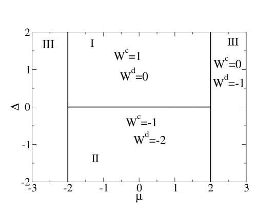
Figure 1: Winding numbers $W^{c}$ and $W^{d}$ of the various phases as a function of chemical potential and pairing amplitude in units of $t$. The winding number respecting to the Hamiltonian in the representation of the $\tilde{d}$ operators takes the values $W^{\tilde{d}}=0,-2,-1$ in phases $II,I,III$, respectively.

The matrix $H_{k}^{d}$ from Eq. (59) allows us to perform a chiral transformation which leads to $q^{d}(k)=-(-t+\Delta)\cos 2k+(t+\Delta)+\mu\cos k+i(-t+\Delta)\sin 2k-i\mu\sin k$. Consider for instance the special point $\mu=0,\Delta=t$. The winding number

$$W^{d}=W^{d}(q^{d}(k))=0$$ (60)

So in terms of the $d$ operators the winding number in the special point indicates a trivial phase. For instance at $\Delta=t,\mu>2t$ we get $W^{d}=1$. So it appears that from the point of view of $W^{d}$ versus $W^{c}$ the model is “dual” and an apparent change of topology takes place.

Since in terms of the $d$-operators the Hamiltonian has first and second neighbors, it is actually like an effective Kitaev model with first and second neighbors. But in this case the model has a phase diagram which is richer with winding numbers $W^{d}=0,\pm 1,\pm 2$. The model is in the BDI class with a $Z$ invariant. For instance, considering $\mu=0$, we can show that it is equivalent to an effective Kitaev model with parameters ($\mu_{2},t_{2},t_{2}^{\prime},\Delta_{2},\Delta_{e}^{\prime}$) where $\mu=0$ implies that $t_{2}=\Delta_{2}=0$ (no nearest-neighbor couplings, being hoppings or pairings). It is well-known that this model has two Majoranas at each edge. With no nearest neighbor couplings the model is like two decoupled chains and so the number of edge modes just doubles. Solving the model in real space with open boundary conditions one obtains two edge modes on each edge.

At point $\mu=0,\Delta=t$ we diagonalized the Kitaev Hamiltonian in real space using Majorana operators and then introducing new fermionic operators. We may achieve something similar at the point $\mu=0,\Delta=-t$. At this point the fermionic operator that diagonalizes the Hamiltonian may be defined as $\tilde{d}_{j}=\frac{-i}{2}(\gamma_{1,j}-i\gamma_{2,j+1})$ This new operator allows to rewrite the Hamiltonian as

$$H=t\sum_{j}\left(2\tilde{d}_{j}^{\dagger}\tilde{d}_{j}-1\right)$$ (61)

the groundstate is obtained taking at each site the zero eigenstate of the operator $\tilde{d}_{j}^{\dagger}\tilde{d}_{j}$. We have the relation

$$\tilde{d}_{j}=\frac{i}{2}\left[c_{j}+c_{j}^{\dagger}+c_{j+1}^{\dagger}-c_{j+1}\right]$$ (62)

Replacing the operators $c_{j},c_{j}^{\dagger}$ by the operators $\tilde{d}_{j},\tilde{d}_{j}^{\dagger}$ at an arbitrary point in the phase diagram, we get a similar expression just replacing $\Delta\rightarrow-\Delta$. We get that in the original topological phase the winding number gives also zero. In Fig. 1 we compare the winding numbers using the various representations showing that their values depend on the set of operators used.

4.2 Berry phase of fermionic problem

Information about the topological properties may also be obtained calculating the Berry phase associated with the eigenstates of the Hamiltonian. We may compare the Berry phases using different representations of the Hamiltonian of the system and therefore different states basis aiming for a more detailed understanding of the relations between different fermionic representations of the problem. We can show that

$$\left(\begin{array}[]{c}d_{k}\\ d_{-k}^{\dagger}\end{array}\right)=U_{k}^{\dagger}\left(\begin{array}[]{c}c_{k}\\ c_{-k}^{\dagger}\end{array}\right),U_{k}=-e^{-\frac{ik}{2}}\left(\begin{array}[]{cc}\sin\frac{k}{2}&i\cos\frac{k}{2}\\ -i\cos\frac{k}{2}&-\sin\frac{k}{2}\\ \end{array}\right)$$ (69)

which implies that $H_{k}^{d}=U_{k}^{\dagger}H_{k}^{c}U_{k}$. Performing the change from $c_{k}$ to $d_{k}$ corresponds to diagonalizing the problem at $\mu=0,\Delta=t$ and performing the change from $c_{k}$ to $\tilde{d}_{k}$ corresponds to diagonalizing the problem at $\mu=0,\Delta=-t$. At the points $\mu=0,\Delta=\pm t$ the eigenvalues are $\pm 2$ and the eigenvectors are

$$\psi_{+}=sgn\left[\cos\frac{k}{2}\right]\left(\begin{array}[]{c}-i\frac{\Delta}{t}\sin\frac{k}{2}\\ \cos\frac{k}{2}\end{array}\right),\psi_{-}=sgn\left[\cos\frac{k}{2}\right]\left(\begin{array}[]{c}\cos\frac{k}{2}\\ -i\frac{\Delta}{t} \sin\frac{k}{2}\end{array}\right)$$ (74)

Taking now $\mu=0$ but any value of $\Delta$, the eigenvalues are

$$\lambda_{\pm}=\pm 2\sqrt{(t\cos k)^{2}+(\Delta\sin k)^{2}}$$ (75)

The eigenvectors are

$$\psi_{+}^{\Delta}=\left(\begin{array}[]{c}\frac{-i2\Delta\sin k}{\sqrt{2\lambda_{+}\left(\lambda_{+}+2t\cos k\right)}}\\ \sqrt{\frac{\lambda_{+}+2t\cos k}{2\lambda_{+}}}\end{array}\right),\psi_{-}^{\Delta}=\left(\begin{array}[]{c}\sqrt{\frac{\lambda_{-}-2t\cos k}{2\lambda_{-}}}\\ \frac{-i2\Delta\sin k}{\sqrt{2\lambda_{-}\left(\lambda_{-}-2t\cos k\right)}}\end{array}\right)$$ (80)

Let us now consider the Berry phase in momentum space (Zak phase). For a given eigenstate $n$ is given by

$$\gamma_{n}=\frac{i}{\pi}\int dk\langle\psi_{n}(k)|\frac{\partial}{\partial k}|\psi_{n}(k)\rangle$$ (81)

As we change variables (or operator descriptions) the states also change. Consider first one abelian change: $|\psi_{n}(k)\rangle\rightarrow e^{i\xi(k)}|\psi_{n}(k)\rangle$. Then we get that

$$\tilde{\gamma}_{n} = \frac{i}{\pi}\int dk\langle\psi_{n}(k)|e^{-i\xi(k)}\frac{\partial}{\partial k}\left[e^{i\xi(k)}|\psi_{n}(k)\rangle\right]$$ (82)

$$= \frac{i}{\pi}\int dk\langle\psi_{n}(k)|\frac{\partial}{\partial k}|\psi_{n}(k)\rangle-\frac{1}{\pi}\int dk\frac{d\xi(k)}{dk}$$

$$= \gamma_{n}+\delta\gamma_{n}$$

If the function $\xi(k)$ is periodic the Zak phase is invariant. This is similar to the well known case of adiabatic transport of some Hamiltonian that depends on some parameter and one considers a cyclic transport: in this case the Berry phase is invariant and observable and is related to the polarization of a system of charges [56].

In our case the state is a vector and in general we have a transformation from $|\psi_{n}\rangle$ to $|\tilde{\psi}_{n}\rangle$: $|\tilde{\psi}_{n}\rangle=U^{\dagger}|\psi_{n}\rangle$, and $\tilde{H}=U^{\dagger}HU$. Then we define

$$\gamma_{n} = \frac{i}{\pi}\int dk\langle\psi_{n}|\partial_{k}|\psi_{n}\rangle$$

$$\tilde{\gamma}_{n} = \frac{i}{\pi}\int dk\langle\tilde{\psi}_{n}|\partial_{k}|\tilde{\psi}_{n}\rangle=\gamma_{n}+\delta\gamma_{n}$$ (83)

where

$$\delta\gamma_{n}=\frac{i}{\pi}\int dk\langle\psi_{n}|U\left(\partial_{k}U^{\dagger}\right)|\psi_{n}\rangle$$ (84)

In general $\delta\gamma_{n}\neq 0$. We can see that

$$\gamma_{n} = \tilde{\gamma}_{n}+\frac{i}{\pi}\int dk\langle\tilde{\psi}_{n}|U^{\dagger}\left(\partial_{k}U\right)|\tilde{\psi}_{n}\rangle$$

$$\tilde{\gamma}_{n} = \gamma_{n}+\frac{i}{\pi}\int dk\langle\psi_{n}|U\left(\partial_{k}U^{\dagger}\right)|\psi_{n}\rangle$$ (85)

Defining a new phase as

$$\tilde{\Gamma}_{n}=\frac{i}{\pi}\int dk\langle\tilde{\psi}_{n}|D_{k}|\tilde{\psi}_{n}\rangle$$ (86)

with

$$D_{k}=\partial_{k}-\left(\partial_{k}U^{\dagger}\right)U$$ (87)

this new phase is invariant in the sense that $\Gamma_{n}=\tilde{\Gamma}_{n}$. The differential operator $D_{k}$ is similar to a covariant derivative and similar to a non-abelian gauge transformation (needed if states are degenerate, although this is not the case here).

Let us now calculate the Zak phase of the state $|\psi_{-}\rangle_{c}$. This is given by

$$\gamma_{-1} = \frac{i}{\pi}\int_{0}^{2\pi}dk\langle\psi_{-}|\partial_{k}|\psi_{-}\rangle_{c}$$ (88)

$$= \frac{i}{\pi}\int_{0}^{2\pi}dk\frac{d}{dk}\left(\ln sgn\left[\cos\frac{k}{2}\right]\right)$$

$$= -1=\gamma_{c}$$

Only the singular part of the wave functions contributes.

Calculate now the Zak phase of the lowest eigenstate of $H_{k}^{d}(\mu=0,\Delta=t)$. This state is simply

$$|\psi_{-}\rangle_{d}=\left(\begin{array}[]{c}0\\ 1\end{array}\right)$$ (91)

and $\gamma_{-1}=\gamma_{d}=0$. Using that $\gamma_{d}=\gamma_{c}+\delta\gamma$ and calculating $\delta\gamma$ we get $\delta\gamma=1$, showing that the change of topology is hidden in the transformation. We have checked that similar results occur in other topological models such as the topologically non-trivial Shockley model.

Singular vs. non-singular transformations

Consider now a transformation between two points in parameter space. For instance, two points at $\mu=0$ but with different values of $\Delta$. Define diagonalized Hamiltonians

$$H_{d}^{\Delta} = U_{\Delta}^{\dagger}H_{\Delta}U_{\Delta}$$

$$H_{d}^{\Delta^{\prime}} = U_{\Delta^{\prime}}^{\dagger}H_{\Delta^{\prime}}U_{\Delta^{\prime}}$$ (92)

The eigenvalues are of the form

$$\lambda_{\Delta}=2\sqrt{(t\cos k)^{2}+(\Delta\sin k)^{2}}$$ (93)

Then $H_{d}^{\Delta^{\prime}}=(\lambda_{\Delta^{\prime}}/\lambda_{\Delta})H_{d}^{\Delta}$ which implies that

$$H_{\Delta^{\prime}}=\frac{\lambda_{\Delta^{\prime}}}{\lambda_{\Delta}}\mathscr{U}^{\dagger}H_{\Delta}\mathscr{U}$$ (94)

Here $\mathscr{U}=U_{\Delta}U_{\Delta^{\prime}}^{\dagger}$. We can relate the eigenstates of the two Hamiltonians defined by $H_{\Delta}|\psi_{\Delta}\rangle=\lambda_{\Delta}|\psi_{\Delta}\rangle$, $H_{\Delta^{\prime}}|\psi_{\Delta^{\prime}}\rangle=\lambda_{\Delta^{\prime}}|\psi_{\Delta^{\prime}}\rangle$ as $|\psi_{\Delta}\rangle=\mathscr{U}|\psi_{\Delta^{\prime}}\rangle$.

The Berry phases may be calculated as

$$\gamma_{\Delta} = \frac{i}{\pi}\int_{0}^{2\pi}dk\langle\psi_{\Delta}|\partial_{k}|\psi_{\Delta}\rangle$$

$$\gamma_{\Delta^{\prime}} = \frac{i}{\pi}\int_{0}^{2\pi}dk\langle\psi_{\Delta^{\prime}}|\partial_{k}|\psi_{\Delta^{\prime}}\rangle$$ (95)

As shown above they are related by

$$\gamma_{\Delta^{\prime}}=\gamma_{\Delta}+\frac{i}{\pi}\int_{0}^{2\pi}dk\langle\psi_{\Delta}|\mathscr{U}\left(\partial_{k}\mathscr{U}^{\dagger}\right)|\psi_{\Delta}\rangle$$ (96)

Consider as an example, $\Delta=1,\Delta^{\prime}=-1$. In these simple cases $\lambda_{\Delta}=\lambda_{\Delta^{\prime}}=1$. The operator is simply given by

$$\mathscr{U}=\frac{1}{2}\left(\begin{array}[]{cc}2\cos k&2i\sin k\\ 2i\sin k&2\cos k\\ \end{array}\right)$$ (99)

Note that $1+\cos k\geq 0$ and no singular part appears. This suggests that $\delta\gamma=0$. Indeed using that

$$|\psi_{-}\rangle(\Delta=1)=sgn\left[\cos\frac{k}{2}\right]\left(\begin{array}[]{c}\cos\frac{k}{2}\\ i\sin\frac{k}{2}\end{array}\right)$$ (102)

and

$$|\psi_{-}\rangle(\Delta=-1)=sgn\left[\cos\frac{k}{2}\right]\left(\begin{array}[]{c}\cos\frac{k}{2}\\ -i\sin\frac{k}{2}\end{array}\right)$$ (105)

we get that $\gamma(\Delta=-1)=-1$, which is the same as for $\Delta=1$.

We may also change the parameters from a topological to a trivial phase. For instance we may consider the point, $A$, $\mu=0,\Delta=t$ and the point, $B$, $\mu>2t,\Delta=0$. The Hamiltonian at this trivial point is diagonal. So the operator that diagonalizes is the identity. Therefore $\mathscr{U}=U_{\Delta=t}$ and as we have seen before $U_{\Delta=1}$ is singular. Therefore $\gamma_{B}=\gamma_{A}+\delta\gamma=-1+1=0$. Note that the winding number distinguishes the phases $I$ and $II$ in the phase diagram. It seems that the Berry phase does not. However, $\gamma=-1=-\pi/\pi$ is the same as $\gamma=1$ since they differ by $2\pi/\pi$.

5 Topology of spin model vs. fermionic representation

The main point however is the change of topology as one transforms from the spin problem to the fermionic dual problem. As established previously [45] the spin model is topologically trivial. In general we can determine the topological properties of an interacting or non-interating system considering that the Hamiltonian depends on a variable and consider that it is cyclic. For instance depends on some angle like $H(\theta)$. The Berry phase is defined as

$$i\gamma=\int_{0}^{2\pi}d\theta A(\theta)$$ (106)

where $A(\theta)=\langle GS(\theta)|\partial_{\theta}|GS(\theta)\rangle$, with $|GS(\theta)\rangle$ the groundstate obtained for a given value of the cyclic parameter. One possible way to introduce a dependence on a cyclic variable is to consider a local twist on a given link (this may be seen as twisted boundary conditions [59]) as

$$S_{i}^{+}S_{j}^{-}+S_{i}^{-}S_{j}^{+}\rightarrow e^{i\theta}S_{i}^{+}S_{j}^{-}+e^{-i\theta}S_{i}^{-}S_{j}^{+}$$ (107)

This method has been used [58] to show that a spin-$1$ chain is topological while half-integer spin chains are topologically trivial. A difficulty arises when the Majorana representation is used since the spin problem is in general an interacting problem and some numerical exact diagonalization is required or a Green’s function approach may be used [60].

Different conventional fermionic representations can be constructed from the Majorana fermions. One possibility is to define a local transformation as $f_{j}=(\gamma_{2,j}+i\gamma_{3,j})/2$ which implies that we can write $i\gamma_{2,j}\gamma_{3,j}=2f_{j}^{\dagger}f_{j}-1$. In terms of these operators we can write that

$$H_{X}=\sum_{j}\left(f_{j}^{\dagger}f_{j}-\frac{1}{2}\right)\left(f_{j+1}^{\dagger}f_{j+1}-\frac{1}{2}\right)$$ (108)

This is an interacting fermionic problem and its topological properties may be obtained imposing twisted boundary conditions and calculating the Berry phase averaging over the twist angle [59, 54]. However, in this representation, since all terms are of the type of number density operators, there is no dependence on the twist angle and the Berry phase vanishes, as expected of a topologically trivial system. The same type of result was obtained before: the diagonalization of Kitaev’s model at the point $\mu=0,\Delta=t$ also allows to write the Hamiltonian in terms of the density operator and therefore the topological invariant vanishes in the same manner.

Also, we may choose a non-local transformation of the type $h_{j}=(\gamma_{2,j}+i\gamma_{3,j+1})/2$. This leads to $i\gamma_{2,j}\gamma_{3,j+1}=2h_{j}^{\dagger}h_{j}-1$ and the Hamiltonian may be written as

$$H_{X} = \frac{1}{4}\sum_{j}\left(2h_{j}^{\dagger}h_{j}-1\right)\left(h_{j-1}h_{j+1}+h_{j-1}h_{j+1}^{\dagger}\right.$$ (109)

$$- \left.h_{j-1}^{\dagger}h_{j+1}-h_{j-1}^{\dagger}h_{j+1}^{\dagger}\right)$$

which is of the type of correlated hoppings and pairings and that requires an explicit calculation of the topological invariant. Note that the two sets of fermionic operators are related by a transformation that is non-trivial and may lead to a change of topology as above for the non-interacting (quadratic) problem. In this case the states are not straightforwardly obtained and the change of the Berry phase involves now a trace over a set of eigenstates that has to be obtained numerically. The relation between the operators $h$ and $f$ in momentum space is given by

$$\left(\begin{array}[]{c}h_{k}\\ h_{-k}^{\dagger}\end{array}\right)=U_{k}^{\dagger}\left(\begin{array}[]{c}f_{k}\\ f_{-k}^{\dagger}\end{array}\right),U_{k}=e^{-\frac{ik}{2}}\left(\begin{array}[]{cc}\cos\frac{k}{2}&i\sin\frac{k}{2}\\ i\sin\frac{k}{2}&\cos\frac{k}{2}\\ \end{array}\right)$$ (116)

This raises the question of possible different topological numbers of the interacting problem, depending on the fermionic representation (see the similarity with Eq. 69).

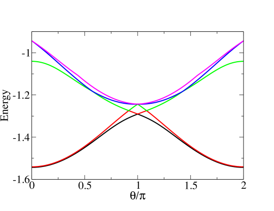
Figure 2: Lowest energy levels obtained by exact diagonalization of a $N=8$ system of fermions that results from the Jordan-Wigner transformation of a spin problem as a function of the angle of the twisted boundary conditions, $\theta$. The parameters of the fermionic problem are $t=1,\Delta=0.5$. ($4t=J_{x}+J_{y}$, $4\delta=J_{x}-J_{y}$).

Mapping and boundary conditions

Let us consider again the spin problem

$$H=-\sum_{j}\left(J_{x}S_{j}^{x}S_{j+1}^{x}+J_{y}S_{j}^{y}S_{j+1}^{y}\right)$$ (117)

The exact diagonalization of this Hamiltonian for a finite system shows that using either periodic boundary conditions (PBC) or open boundary conditions (OBC) the groundstate is a singlet in general. For the $X$ model with $J_{y}=0$ the groundstate is doubly degenerate for both sets of boundary conditions. Imposing twisted boundary conditions one may calculate the Berry phase and it vanishes confirming that the system is topologically trivial.

Consider now the traditional Jordan-Wigner transformation to spinless fermions. This is straightforward for OBC. However, as is well known, choosing PBC for the spins, $S_{N+1}=S_{1}$, translates into the fermionic problem as

$$c_{N+1}=e^{i\pi\hat{N}_{F}}c_{1}=c_{1}e^{i\pi(\hat{N}_{F}-\hat{n}_{1})}$$ (118)

where $\hat{N}_{F}$ is the operator that counts the total number of fermions, $c$. Diagonalizing the many-body fermionic problem that results from the Jordan-Wigner transformation and considering OBC one obtains the same energy levels as for the original spin problem, as expected. Implementing periodic boundary conditions in addition to the relation imposed by the Jordan-Wigner transformation leads to the same spectrum as for the spin problem with PBC. The exact diagonalization of the many-body problem is carried out using an occupation number representation of the Hilbert space.

Consider now the Kitaev model by itself without reference to its spin origin. Diagonalization of the many-body problem with OBC leads naturally to the same spectrum selecting the appropriate values of $t=1.5,\Delta=0.5$ for $J_{x}=1,J_{y}=0.5$. Considering now the Kitaev model with strict periodic boundary conditions $c_{N+1}=c_{1}$ leads however to a different energy spectrum, in particular a different groundstate energy (at least for a finite system).

Imposing twisted boundary conditions in the fermionic model that is obtained by the Jordan-Wigner transformations leads to a Berry phase that vanishes, as for the original spin problem. In Fig. 2 we show the lowest many-body energy eigenvalues as a function of the twist angle, $\theta$, for $t=1,\Delta=0.5$. Note that the groundstate has no degeneracy with the first excited state except perhaps at $\theta=\pi$.

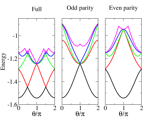
Figure 3: Lowest energy levels of a $N=8$ system of fermions describing Kitaev’s model as a function of the angle of the twisted boundary conditions, $\theta$. The parameters of the fermionic problem are $t=1,\Delta=0.5$. In the middle and right panels a subset of states of given parity is considered. The Hamiltonian does not couple the two subsectors.

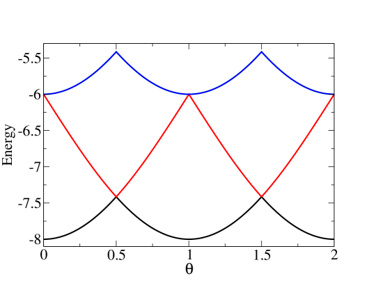
Figure 4: Lowest energy levels of a $N=8$ system of fermions describing Kitaev’s model as a function of the angle of the twisted boundary conditions, $\theta$. The parameters of the fermionic problem are $t=1,\Delta=1$.

Consider now the Kitaev model with strict PBC, once again solved as a many-body problem. In Fig. 3 and in Fig. 4 we show the lowest many-body eigenvalues as a function of the twist angle, $\theta$. In Fig. 3 we consider $t=1,\Delta=0.5$ and in Fig. 4 we consider $t=1,\Delta=1$. Note the degeneracy of the lowest energy state with the first excited state at $\theta=\pi/2$. In Fig. 3 we show in addition to the full energy spectrum (left panel) the spectra for the two fermionic parities. Since the Hamiltonian conserves the fermionic parity (since it only couples subspaces where wither the number of fermions does not change or changes by two fermions) the Hamiltonian may be diagonalized by blocks. As shown before, the overall groundstate at $\theta=0$ has odd parity. At $\theta=\pi/2$ the spectra cross and there is a degeneracy. If one now calculates the Berry phase one finds that it is neither zero nor $\pi$ (mod($2\pi$). The Berry phase is well defined if there is a gap throughout the twist angle space.

However, as is well known, and we have rederived above, using the single particle approach and using a momentum space description, the Berry phase is easily calculated. We may then consider a real space description using twisted boundary conditions as for the full many-body problem but considering the many-body states as Slater determinants of single-particle states. In Appendix C the topological phase is confirmed.

In summary, the apparent change of topology, when the mapping from a spin problem to the Kitaev model is carried out, is the result of different boundary conditions (when OBC are not used) that lead to a difference in the Berry phase with respect to the original spin problem. The calculation of the Berry phase for the many-body fermionic Kitaev problem is inconclusive due to degeneracies as a function of the twisted boundary conditions. The analysis of the Berry phase of the dual interacting fermionic problems that results from the representation of the spin operators by different fermionic representations is further complicated by degeneracies introduced due to the enlargement of the Hilbert space.

6 Conclusions

In this work we have considered a representation of fermionic and spin operators in terms of Majorana fermions and have used it systematically to relate the two types of problems. We focused on mappings between the two types of systems with particular emphasis on the relation of the topological properties as a result of the unitary transformations that lead from one problem to another and on the effect of boundary conditions. The simpler case of a unitary transformation that relates two fermionic problems was considered and the singular or non-singular nature of the transformation determines the change of topological invariants. The analysis of the change of topological properties due to the mapping between the spin problem and its fermionic representation is, however, more complex, since the calculation of a topological invariant of the interacting problem in general requires a numerical solution. This has been performed using exact diagonalization of the system in the presence of twisted boundary conditions. In the case of the mapping from the $XY$ model to the Kitaev model using the appropriate boundary conditions in the fermionic problem leads to a non-topological system (as the original spin problem) while the Kitaev model has topological phases.

The various types of unitary transformations allow mappings to different problems with preserved or changed statistics and in general allow the replacement of interacting terms by free terms and vice-versa. This property has been used in different contexts in the literature to address the problem of strongly interacting systems even though in general some enlargement of the Hilbert space occurs. Another interesting problem may be the effect of interactions in the Kitaev model and its possible mapping to spin problems [61].

Acknowledgments

PDS acknowledges several discussions with Stellan Östlund, partial support and hospitality by Henrik Johannesson and by the Department of Physics of Gothenburg University grant 621-2014-5972 (Swedish Research Council), where the initial stages of this work were carried out. The authors also acknowledge discussions with Bruno Amorim, Bruno Mera, Rubem Mondaini and Yan Chao Li.

Partial support from FCT through grant UID/CTM/04540/2013 is acknowledged.

Appendix A Jordan-Wigner transformation and Kitaev chain

We may consider a spin-$1/2$ system that has anisotropy in the $XY$ plane described by the Hamiltonian

$$H_{XY}=-\sum_{j=1}^{N}\left(J_{x}S^{x}_{j}S^{x}_{j+1}+J_{y}S^{y}_{j}S^{y}_{j+1}\right)$$ (119)

Defining $S^{x}=\left(S^{+}+S^{-}\right)/2;S^{y}=\left(S^{+}-S^{-}\right)/(2i)$ we can write that

$$H_{XY} = -\frac{1}{4}\sum_{j}\left[\left(J_{x}-J_{y}\right)\left(S^{+}_{j}S^{+}_{j+1}+S^{-}_{j}S^{-}_{j+1}\right)\right]$$ (120)

$$-\frac{1}{4}\sum_{j}\left[\left(J_{x}+J_{y}\right)\left(S^{+}_{j}S^{-}_{j+1}+S^{-}_{j}S^{+}_{j+1}\right)\right]$$

This is an interacting quantum problem that is well known to be diagonalizable. A possible way consists in performing the transformation from the spin operators to spinless fermionic operators as [17]

$$S^{+}_{j} = c^{\dagger}_{j}e^{i\pi\sum_{n=1}^{j-1}c^{\dagger}_{n}c_{n}}$$

$$S^{-}_{j} = e^{-i\pi\sum_{n=1}^{j-1}c^{\dagger}_{n}c_{n}}c_{j}$$ (121)

leading to

$$H_{XY} = -\frac{1}{4}\sum_{j}\left[\left(J_{x}-J_{y}\right)\left(c^{\dagger}_{j}c^{\dagger}_{j+1}+c_{j+1}c_{j}\right)\right]$$ (122)

$$-\frac{1}{4}\sum_{j}\left[\left(J_{x}+J_{y}\right)\left(c^{\dagger}_{j}c_{j+1}+c^{\dagger}_{j+1}c_{j}\right)\right]$$

This model is related to the Kitaev model [16] (at vanishing chemical potential) if we rewrite it as

$$H=-t\sum_{j}\left(c^{\dagger}_{j}c_{j+1}+c^{\dagger}_{j+1}c_{j}\right)+\Delta\sum_{j}\left(c_{j}c_{j+1}+c^{\dagger}_{j+1}c^{\dagger}_{j}\right)$$ (123)

choosing $t=(J_{x}+J_{y})/4;\Delta=(J_{x}-J_{y})/4$. Therefore if $J_{y}=0$ we get that $\Delta=t$ and if $J_{x}=J_{y}$ we get that $\Delta=0$. If $\Delta=0$ the spectrum is gapless and if $\Delta\neq 0$ there is a gap in the system. Therefore, $\Delta=0$ is a critical point that separates two gapped phases.

Consider now the addition of a chemical potential term, $\mu\neq 0$. This can be traced back to a magnetic field in the $XY$ model and adds a term of the type $-\mu\sum_{j}\left(c^{\dagger}_{j}c_{j}-\frac{1}{2}\right)$. For any $|\mu|>2t$ the band is either empty or full. For $|\mu|<2t$ the spectrum is gapless if $\Delta=0$ and there is a gap if $\Delta$ is finite.

If $J_{x},J_{y}>0$, the spin system is ferromagnetic. If $J_{x}>J_{y}$ ($J_{x}<J_{y}$) the spins order at zero temperature along the $x$ direction ($y$ direction). If $J_{x}=J_{y}$ the system is isotropic and critical with power law correlation functions. In the corresponding Kitaev model the critical regime is the non-superconducting tight-binding model. If $J_{x}>J_{y}\rightarrow\Delta>0$ and $J_{x}<J_{y}\rightarrow\Delta<0$, and in both cases there is a gap that corresponds in the spin problem to the Landau like quasi-long-range order.

The spinless fermionic operators may be written in terms of Hermitian operators, Majorana operators, as $c_{j}=\frac{1}{2}\left(\gamma_{1,j}+i\gamma_{2,j}\right)$. In terms of these operators the Hamiltonian can be written as

$$H=\frac{i}{2}\sum_{j}\left[\left(-t+\Delta\right)\gamma_{1,j}\gamma_{2,j+1}+\left(t+\Delta\right)\gamma_{2,j}\gamma_{1,j+1}\right]-\frac{i}{2}\mu\sum_{j}\gamma_{1,j}\gamma_{2,j}$$ (124)

Note that at some particular point $(\mu=0,t=\Delta)$ the Hamiltonian becomes quite simple

$$H=it\sum_{j}\gamma_{2,j}\gamma_{1,j+1}$$ (125)

If we define non-local operators [16] $d_{j}^{\dagger}=\frac{1}{2}\left(\gamma_{2,j}-i\gamma_{1,j+1}\right)$ they are related to the other fermionic operators by

$$d_{j}^{\dagger}=\frac{1}{2}\left[-i(c_{j}-c_{j}^{\dagger})-i(c_{j+1}+c_{j+1}^{\dagger})\right]$$ (126)

We may note that $2d_{j}^{\dagger}d_{j}-1=i\gamma_{2,j}\gamma_{1,j+1}$ which leads to

$$H=t\sum_{j=1}^{N-1}\left(2d_{j}^{\dagger}d_{j}-1\right)$$ (127)

If we use open boundary conditions (OBC) we see immediately that $d_{N}^{\dagger}d_{N}$ does not appear in the Hamiltonian, which leads to a degenerate groundstate ($d_{N}^{\dagger}d_{N}=0,1$) with two Majoranas.

If we use periodic boundary conditions (PBC) we just need to add this term ($d_{N}^{\dagger}d_{N}$):

$$H=t\sum_{j=1}^{N}\left(2d_{j}^{\dagger}d_{j}-1\right)$$ (128)

Note that $d_{N}=\frac{i}{2}(c_{N}^{\dagger}-c_{N}+c_{1}+c_{1}^{\dagger})$. Therefore, $d_{N}^{\dagger}+d_{N}=i(c_{N}^{\dagger}-c_{N})$ and $d_{N}-d_{N}^{\dagger}=i(c_{1}+c_{1}^{\dagger})$. The groundstate of the $d$ operators is the groundstate of the system, at this special point

$$|GS\rangle=|n_{d}=0;n_{d}=0;\cdots;n_{d}=0;\cdots\rangle$$ (129)

written in terms of the $d$ operators.

We may now define two states with different fermionic parities [53]

$$|\psi^{0}_{even}\rangle = \left(\prod_{j=1}^{N-1}d_{j}d_{j}^{\dagger}\right)|0\rangle$$

$$|\psi^{0}_{odd}\rangle = \left(\prod_{j=1}^{N-1}d_{j}d_{j}^{\dagger}\right)c_{N}^{\dagger}|0\rangle$$ (130)

where $|0\rangle=|0\rangle_{N}\cdots|0\rangle_{1}$, with $c_{j}|0\rangle_{j}=0$. These states $|\psi^{0}_{even}\rangle$ and $|\psi^{0}_{odd}\rangle$ have no excitations of the $d$ operators.

These states can be represented in terms of the original $c$ fermionic operators of the model as shown in Ref. [53]

$$|\psi_{0}^{even}\rangle = \prod_{j=1}^{N}\left(1+c_{j}^{\dagger}\right)_{even}|0\rangle_{c}$$

$$|\psi_{0}^{odd}\rangle = \prod_{j=1}^{N}\left(1+c_{j}^{\dagger}\right)_{odd}|0\rangle_{c}$$ (131)

where only even or odd powers of $c$ operators contribute. It was also shown that [53]

$$d_{N}|\psi_{0}^{odd}\rangle=0$$ (132)

and

$$d_{N}^{\dagger}|\psi_{0}^{odd}\rangle=-i|\psi_{0}^{even}\rangle$$ (133)

One can conclude that the groundstate is non-degenerate and has odd parity.

Appendix B Generalized $SU(2)$ algebras and Majorana operators

Considering the combinations $I_{\pm}=\frac{1}{2}(I\pm I_{3})$, and $\Sigma^{\pm}_{i}=\frac{1}{2}(\mathscr{S}_{i}\pm\gamma_{i})$ one finds that the product of two operators of different signs vanishes and that

$$I_{\pm}^{2} = I_{\pm}$$ (134)

$$\Sigma^{+}_{i}\Sigma^{+}_{j} = \delta_{ij}I_{+}+i\epsilon_{ijk}\Sigma^{+}_{k}$$ (135)

$$\Sigma^{-}_{i}\Sigma^{-}_{j} = \delta_{ij}I_{-}+i\epsilon_{ijk}\Sigma^{-}_{k}$$ (136)

i.e. they commute and satisfy two separate $SU(2)$ algebras, with $I_{\pm}$ as the identities. One also has $(\vec{\Sigma}^{\pm})^{2}=3I$ and $\vec{\Sigma}^{+}\cdot\vec{\Sigma}^{-}=0$.

Additionally, besides the projectors $I_{\pm}$, it is also sometimes useful to use the operators $P^{+\pm}_{\vec{n}}=\frac{1}{2}(I_{+}\pm\vec{n}\cdot\vec{\Sigma^{+}})$ and $P^{-\pm}_{\vec{n}}=\frac{1}{2}(I_{-}\pm\vec{n}\cdot\vec{\Sigma^{-}})$, which, for a given unit vector $\vec{n}$, are also projectors, i.e. they satisfy $P_{a}P_{b}=\delta_{ab}P_{a}$, with $a,b=\pm\pm$. Finite operators involving projectors are generally given by

$$e^{i\alpha P}=I+(e^{i\alpha}-1)P=(I-P)+e^{i\alpha}P$$ (137)

for a single operator, and

$$e^{i\sum_{i}\alpha_{i}P_{i}}=I+\sum_{i}(e^{i\alpha_{i}}-1)P_{i}=(I-\sum_{i}P_{i})+\sum_{i}e^{i\alpha_{i}}P_{i}$$ (138)

for several operators. When $\sum_{i}P_{i}=I$ the first term vanishes and one finds the usual decomposition of an exponential operator in its own complete basis, namely for the Boltzmann factor. In particular, one has

$$e^{i\alpha I_{\pm}}=I+(e^{i\alpha}-1)I_{\pm}=I_{\mp}+e^{i\alpha}I_{\pm}$$ (139)

The finite operators of the $SU(2)$ generators are given by

$$e^{i\frac{\theta}{2}\vec{n}\cdot\vec{\gamma}} = \cos\frac{\theta}{2}I+i\sin\frac{\theta}{2}\vec{n}\cdot\vec{\gamma}$$ (140)

$$e^{i\frac{\theta}{2}\vec{n}\cdot\vec{\mathscr{S}}} = \cos\frac{\theta}{2}I+i\sin\frac{\theta}{2}\vec{n}\cdot\vec{\mathscr{S}}$$ (141)

$$e^{i\frac{\theta}{2}\vec{n}\cdot\vec{\Sigma}_{\pm}} = I_{\mp}+\cos\frac{\theta}{2}I_{\pm}+i\sin\frac{\theta}{2}\vec{n}\cdot\vec{\Sigma}_{\pm}$$ (142)

with $\vec{n}$ a unit vector, $\vec{n}^{2}=1$. In the last equation, the first term reflects the existence of two separate $SU(2)$ algebras, each with its own identity. Finally,

$$e^{i\frac{\theta}{2}I_{3}}=\cos\frac{\theta}{2}+i\sin\frac{\theta}{2}I_{3}$$ (143)

More general operators can be obtained from these results, in particular using the last two equations and eq. (139), using $\vec{n}\cdot\vec{\mathscr{S}}=\vec{n}\cdot\vec{\Sigma}_{+}+\vec{n}\cdot\vec{\Sigma}_{-}$, $\vec{n}\cdot\vec{\gamma}=\vec{n}\cdot\vec{\Sigma}_{+}-\vec{n}\cdot\vec{\Sigma}_{-}$ and $I_{3}=I_{+}-I_{-}$

The action of finite operations, namely of unitary operations, on the generators, are similar to the usual expression for the rotations of vectors, but paying due attention to the existence of the two $SU(2)$ commuting (and annihilating) algebras and to the parity of the different operators in terms of the Majorana operators.

Appendix C Berry phase of Kitaev model: real space single-particle description

The twisted boundary conditions for the wave functions of the Bogoliubov-de Gennes equations are taken as

$$u_{n}^{\theta}(j+Na) = e^{i\theta}u_{n}^{\theta}(j)$$

$$v_{n}^{\theta}(j+Na) = e^{-i\theta}v_{n}^{\theta}(j)$$ (144)

The problem is solved for a finite system with size $N$, typically taken large enough. The groundstate may be represented by a matrix

$$\Phi_{\theta}=\left(\begin{array}[]{cccc}\phi_{r_{1}}^{1,\theta}&\phi_{r_{1}}^{2,\theta}&\cdots&\phi_{r_{1}}^{M,\theta}\\ \phi_{r_{2}}^{1,\theta}&\phi_{r_{2}}^{2,\theta}&\cdots&\phi_{r_{2}}^{M,\theta}\\ \cdots&\cdots&\cdots&\cdots\\ \phi_{r_{N}}^{1,\theta}&\phi_{r_{N}}^{2,\theta}&\cdots&\phi_{r_{N}}^{M,\theta}\\ \end{array}\right)$$ (145)

where $M$ is the number of occupied single-particle states and $r_{j}$ is the coordinate of site $j$. Also, $\phi_{j}^{T}=(u_{j},v_{j})^{T}$, where $T$ is the transpose of the vector. The lattice Berry phase may then be obtained as

$$i\gamma=\sum_{l=1}^{L}\ln A_{l}(\theta)$$ (146)

where $L$ is the number of $\theta$ points and $A_{l}(\theta)=\langle GS(\theta_{l})|GS(\theta_{l+1})\rangle$. Since each state is now a many-body state given by a Slater determinant, the overlaps between two states with different boundary conditions are given by

$$\langle\Psi^{\theta}|\Psi^{\theta^{\prime}}\rangle=det\left(\Phi_{\theta}^{\dagger}\Phi_{\theta^{\prime}}\right)$$ (147)

and the Berry phase is obtained by

$$\gamma=-i\sum_{l=1}^{L}\ln\lambda_{p}$$ (148)

where $\lambda_{p}$ are the eigenvalues of the matrix product $\left(\Phi_{\theta_{l}}^{\dagger}\Phi_{\theta_{l+1}}\right)$. Considering a large enough system size and discretization of the twist angle between zero and $2\pi$, leads to the expected result that the Berry phase is $\pi$ in the topological regime previously identified and vanishes in the topologically trivial region.

The degeneracy of the many-body spectrum at twist angle $\theta=\pi/2$ is understood looking at the single particle spectrum, at the same twist angle. Indeed choosing $\theta=\pi/2$ leads to Majorana states of vanishing energy at the edges of the system and therefore to the degeneracy of the many-body spectrum. Interestingly this choice of twisted boundary condition may be seen considering a ring pierced by a flux of $\pi/2$. Note that the boundary condition is then $c_{N+1}=\pm ic_{1}$.

References

References

- [1] S. Östlund and E. Mele, Phys. Rev. B 44, 12413 (1991).
- [2] S. Östlund, M. Granath, Phys. Rev. Lett. 96, 066404 (2006).
- [3] B. Kumar, Phys. Rev. B 77, 205115 (2008).
- [4] A. Angelucci, Phys. Rev. B 51, 11580 (1995).
- [5] S.E. Barnes, J. Phys. F: Met. Phys. 6, 1375 (1976), J. Phys. F: Met. Phys. 7, 2637 (1977).
- [6] P. Coleman, Phys. Rev. B 29, 3035 (1984), 35, 5072 (1987).
- [7] P.A. Lee, N. Nagaosa and X.G. Wen, Rev. Mod. Phys. 78, 17 (2006).
- [8] A.J. Millis and P.A. Lee, Phys. Rev. B 35, 3394 (1987).
- [9] G. Kotliar and A. Ruckenstein, Phys. Rev. Lett. 57, 1362 (1986).
- [10] V. Dorin and P. Schlottmann, Phys. Rev. B 46, 10800 (1992).
- [11] C.L. Kane, P.A. Lee and N. Read, Phys. Rev. B 39, 6880 (1989).
- [12] D.P. Arovas and A. Auerbach, Phys. Rev. B 38, 316 (1988), A. Auerbach and D.P. Arovas, Phys. Rev. Lett. 61, 617 (1988), A. Auerbach and B. E. Larson, Phys. Rev. B 43, 7800 (1991).
- [13] A. Auerbach, “Interacting electrons and quantum magnetism” (Springer-Verlag, New York, 1998).
- [14] E. Lieb, T. Schultz and D. Mattis, Ann. of Phys. 16, 407 (1961).
- [15] B. K. Chakrabarti, A. Dutta and P. Sen, “Quantum Ising phases and transitions in transverse Ising models” (Springer-Verlag, 1996).
- [16] A.Y. Kitaev, Physics-Uspekhi 44, (10S) 131 (2001).
- [17] P. Jordan and E. Wigner, Z. Phys. 47, 631 (1928), Y.R. Wang, Phys. Rev. B 46, 151 (1992).
- [18] J.R. Schrieffer and P.A. Wolff, Phys. Rev. 149, 491 (1966).
- [19] A.O. Gogolin, A.A. Nersesyan and A.M. Tsvelik, “‘Bosonization and Strongly Correlated Systems” (Cambridge, 1998); M. Stone ed., “Bosonization” (World Scientific, 1994).
- [20] F.A. Berezin and M.S. Marinov, Annals of Phys. 104, 336 (1977), JETP Lett. 21, 320 (1975).
- [21] V.R. Vieira, Phys. Rev. B 23, 6043 (1981).
- [22] P.D.S. Sacramento and V.R. Vieira, J. Phys. C 21, 3099 (1988).
- [23] A.M. Tsvelik, Phys. Rev. Lett. 69, 2142 (1992).
- [24] P. Coleman, E. Miranda, A. Tsvelik, Phys. Rev. B 49, 8955 (1994).
- [25] B. S. Shastry, D. Sen, Phys. Rev. B 55, 2988 (1997).
- [26] V.R. Vieira, Phys. Rev. B 39, 7174 (1989).
- [27] V. Turkowski, V.R. Vieira and P.D. Sacramento, Physica A 327, 461 (2003), V.M. Turkowski, P.D. Sacramento and V.R. Vieira, Phys. Rev. B 73, 214437 (2006).
- [28] M. Bazanella, J. Nilsson, arXiv:1405.5176.
- [29] M. Bazzanella, Ph.D. Thesis, University of Gothenburg (2014), https://gupea.ub.gu.se/handle/2077/37148.
- [30] J. Alicea, Rep. Prog. Phys. 75, 076501 (2012).
- [31] J. D. Sau, R.M. Lutchyn, S. Tewari, and S. Das Sarma, Phys. Rev. Lett. 104, 040502 (2010), Jay D. Sau, Sumanta Tewari, Roman M. Lutchyn, Tudor D. Stanescu, and S. Das Sarma, Phys. Rev. B 82, 214509 (2010), V. Mourik, K. Zuo, S. M. Frolov, S. R. Plissard, E. P. A. M. Bakkers, and L. P. Kouwenhoven, Science 336, 1003 (2012).
- [32] S. Nadj-Perge, I. K. Drozdov, B. A. Bernevig, and Ali Yazdani, Phys. Rev. B 88, 020407(R) (2013), Stevan Nadj-Perge, Ilya K. Drozdov, Jian Li, Hua Chen, Sangjun Jeon, Jungpil Seo, Allan H. MacDonald, B. Andrei Bernevig and Ali Yazdani, Science 346, 602 (2014).
- [33] H.A. Kramers and G.H. Wannier, Phys. Rev. 60, 252 and 263 (1941).
- [34] E. Cobanera, G. Ortiz, Z. Nussinov, Adv. in Phys. 60, 679 (2011).
- [35] S.-M. Huang, W.-F. Tsai, C.-H. Chung, and C.-Y. Mou, Phys. Rev. B 93, 054518 (2016).
- [36] E. Cobanera, G. Ortiz, Phys. Rev. B 92, 155125 (2015).
- [37] M.Z. Hasan and C.L. Kane, Rev. Mod. Phys. 82, 3045 (2010).
- [38] X.-L. Qi and S.-C. Zhang, Rev. Mod. Phys. 83, 1057 (2011).
- [39] T.H. Hanson, V. Oganesyan, S.L. Sondhi, Annals of Phys. 313, 497 (2004).
- [40] F.D.M. Haldane, Phys. Lett. 93A, 464 (1983), Phys. Rev. Lett. 50, 1153 (1983).
- [41] I. Affleck, T. Kennedy, E. H. Lieb, and H. Tasaki, Phys. Rev. Lett. 59, 799 (1987), Comm. Math. Phys. 115, 477 (1988).
- [42] M. den Nijs and K. Rommelse, Phys. Rev. B 40, 4709 (1989).
- [43] T. Kennedy and H. Tasaki, Phys. Rev. B 45, 304 (1992).
- [44] M. Oshikawa, J. Phys. Cond. Matt. 4, 7469 (1992).
- [45] F. Pollmann, E. Berg, A. M. Turner, and M. Oshikawa, Phys. Rev. B 85, 075125 (2012).
- [46] E. Cobanera, G. Ortiz, Z. Nussinov, Phys. Rev. B 87, 041105(R) (2013).
- [47] Z. Nussinov, G. Ortiz, Annals of Phys. 324, 977 (2009).
- [48] A. Kitaev and J. Preskill, Phys. Rev. Lett. 96, 110404 (2006), M. Levin and X.G. Wen, Phys. Rev. Lett. 96, 110405 (2006).
- [49] X.-G. Wen, Adv. Phys. 44, 405 (1995).
- [50] N. Read and D. Green, Phys. Rev. B 61, 10267 (2000).
- [51] R. Brauer and H. Weyl, Amer. J. Math., 57 425 (1935).
- [52] S. Ryu, A.P. Schnyder, A. Furusaki and A.W.W. Ludwig, New Journal of Physics, 12, 1 (2010).
- [53] M. Greiter, V. Schnells, R. Thomale, Annals of Phys. 351, 1026 (2014).
- [54] W. C. Yu, Y. C. Li, P. D. Sacramento and H.-Q. Lin, Phys. Rev. B 94, 245123 (2016).
- [55] S.S. Pershoguba and V.M. Yakovenko, Phys. Rev. B 86, 075304 (2012).
- [56] D. Xiao, M.-C. Chang and Q. Niu, Rev. Mod. Phys. 82, 1959 (2010).
- [57] M. Sato and S. Fujimoto, Phys. Rev. B 79, 094504 (2009).
- [58] T. Hirano, H. Katsura, and Y. Hatsugai, Phys. Rev. B 77, 094431 (2008).
- [59] D.J. Thouless, M. Kohmoto, M.P. Nightingale and M. den Nijs, Phys. Rev. Lett. 49, 405 (1982).
- [60] V. Gurarie, Phys. Rev. B 83, 085426 (2011), S.R. Manmana, A.M. Essin, R.M. Noack and V. Gurarie, Phys. Rev. B 86, 2015119 (2012).
- [61] H. Katsura, D. Schuricht, M. Takahashi, Phys. Rev. B 92, 115137 (2015).