Bayesian Transformed GARMA Models

Abstract

Transformed Generalized Autoregressive Moving Average (TGARMA) models were recently proposed to deal with non-additivity, non-normality and heteroscedasticity in real time series data. In this paper, a Bayesian approach is proposed for TGARMA models, thus extending the original model. We conducted a simulation study to investigate the performance of Bayesian estimation and Bayesian model selection criteria. In addition, a real dataset was analysed using the proposed approach.

Keywords: Generalized ARMA model, Bayesian inference, Transformations, gamma distribution, inverse Gaussian distribution

1 Introduction

Generalized Autoregressive Moving Average (GARMA) models extend the classical ARMA time series models and have been around since the seminal work of Benjamin et al. (2003). GARMA models are designed to accommodate time series data (either discrete or continuous) associated with distributions in the exponential family. However, to ensure that the usual assumptions for GARMA models hold a transformation of the original data may be necessary. This is the idea behind the so called Transformed Generalized Autoregressive Moving Average (TGARMA) models proposed recently by de Andrade et al. (2016b) which provide a great deal of flexibility in modeling time series data with possible non-additivity, non-normality and heteroscedasticity. The authors applied maximum likelihood and bootstrap methods for parameter estimation and prediction. The main motivation for the present work is to provide a fully Bayesian approach to estimate parameters, compare models and make predictions in TGARMA models.

In the recent literature, transformations have been shown as a good alternative to reduce certain anomalies in the data. For example, Hamasaki and Kim (2007) described a Box and Cox power-transformation to confined and censored nonnormal responses in regression, da Silva et al. (2011) proposed the use of Box-Cox transformations and regression models to deal with fecal egg count data and Gillard (2012) presented a study using a Box-Cox family of transformations and highlight problems with asymmetry in the transformed data. Castillo and F.G. (2013) commented about many fields where the Box-Cox transformation can be used, and also proposed a method to improve the forecasting models. Ahmad et al. (2015) combined Box-Cox transformation and bootstrapping ideas in one single algorithm where the transformation was used to ensure the data is normally distributed while bootstraping allowed to deal with small and limited sample size data.

de Andrade et al. (2016b) proposed the estimation of the transformation parameter $\lambda$ via profile likelihood (PL). Zhu and Ghodsi (2006) presented a procedure to dimensionality selection maximizing a profile likelihood function. Huang et al. (2013) proposed an efficient equation for estimating the index parameter and unknown link function using adaptive profile-empirical-likelihood inferences. Finally, Cole et al. (2014) provide a primer on maximum likelihood, profile likelihood and penalized likelihood which have proven useful in epidemiologic research.

In the Bayesian approach, computational methods based on Markov chain Monte Carlo (MCMC) can be utilized to address the complexity of the profile likelihood. Thus, our main contribution concerns inference under the Bayesian framework providing efficient MCMC procedures to evaluate the joint posterior distribution of model parameters. Recently, de Andrade et al. (2016a) presented a Bayesian approach for GARMA models, indicating advantages of using Bayesian methods. This paper builds upon previous work and extends the fully Bayesian approach to transformed GARMA models by assingning a prior distribution to the transformation parameter which is then embedded in the estimation process. Prior constraints on $\lambda$ are easily incorporated and these are guaranteed to be valid in the posterior distribution. We also use Bayesian information criteria to compare competing models. Finally, properties of MCMC were used to improve predictions and construct prediction intervals.

The rest of the paper is organized as follows. In Section 2 we present the main concepts associated with TGARMA models. Section 3 defines the Bayesian approach for this new class of models. Section 4 contains the simulation study and Section 5 presents the real data analysis on Swedish fertility rates. Finally, Section 6 gives concluding remarks.

2 Transformed Generalized Autoregressive Moving Average (TGARMA) Model

Box and Cox (1964) commented that many important results in statistical analysis follow from the assumption that the population being sampled or investigated is normally distributed with a common variance and additive error structure. For this reason, these authors presented a transformation called Box-Cox power transformation that has generated a great deal of interests, both in theoretical work and in practical applications. This family has been modified by Cox (1981) to take account of the discontinuity at $\lambda=0$, such that,

$$y_{t}^{(\lambda)}=\left\{\begin{array}[]{ll}\frac{(Y_{t}^{\lambda}-1)}{\lambda};\lambda\neq 0\\ \log(Y_{t});\lambda=0\end{array}\right.$$

Sakia (1992), Manly (1976) and Draper and Cox (1969) discuss others transformation which have the same goal, namely to reduce anomalies in the data. In most applications, the literature recommends the use of Box-Cox power transformation as a general transformation. In the next section we present the TGARMA approach to time series data using this Box-Cox power transformation in conection with the exponential family of distributions.

2.1 Model definition

The TGARMA model specifies the conditional distribution of each transformed observation $y_{t}^{(\lambda)}$, for $t=1,\ldots,n$ given the previous information set, defined as ${F}_{t-1}^{(\lambda)}=(y_{1}^{(\lambda)},\ldots,y_{t-1}^{(\lambda)},\mu_{1},\ldots,\mu_{t-1})$. This conditional density belongs to exponential family and is given by,

$$f(y_{t}^{(\lambda)}|{F}_{t-1}^{(\lambda)})=\exp\left(\frac{y_{t}^{(\lambda)}\alpha_{t}-b(\alpha_{t})}{\varphi}+d(y_{t}^{(\lambda)},\varphi)\right),$$ (2.1)

where $\alpha_{t}$ and $\varphi$ are the canonical and scale parameters, respectively. Moreover $b(\cdot)$ and $d(\cdot)$ are specific functions that define the particular exponential family. The conditional mean and conditional variance of $y_{t}^{(\lambda)}$ given ${F}_{t-1}^{(\lambda)}$ are represented as,

$$\mu_{t}=b^{\prime}(\alpha_{t}) = E(y_{t}^{(\lambda)}|{F}_{t-1}^{(\lambda)})$$

$$Var(y_{t}^{(\lambda)}|{F}_{t-1}^{(\lambda)}) = \varphi{b^{\prime\prime}}(\alpha_{t}),~{}t=1,\ldots,n.$$

Following the Generalized Linear Models (GLM) approach the conditional mean $\mu_{t}$ is related to the linear predictor $\eta_{t}$ by a twice differentiable one-to-one monotonic function $g$, called $link$ $function$. In general, a set of covariates x can be included into the linear predictor. However, our main interest here is to take into account time series features of the data and this is accomplished by adding additional components allowing for autoregressive moving average terms. In such a case our model will have the following form,

$$g(\mu_{t})=\eta_{t}=x^{\prime}_{t}\beta+\sum_{j=1}^{p}\phi_{j}\{g(y_{t-j}^{(\lambda)})-x^{\prime}_{t-j}\beta\}+\sum_{j=1}^{q}\theta_{j}\{g(y_{t-j}^{(\lambda)})-\eta_{t-j}\}.$$ (2.2)

where the model orders $p$ and $q$ are identified using Baysian information criteria. The TGARMA($p,q$) model in its most general form is defined by equations (2.1) and (2.2). We note however that it may be necessary to replace $y_{t}^{(\lambda)}$ with some $y_{t}^{(\lambda^{new})}$ in (2.2) to avoid the possible non-existence of $g(y_{t}^{(\lambda)})$ for certain values of $y_{t}^{(\lambda)}$.

In this paper we will consider Box-Cox transformations in two important continuos GARMA models: gamma and inverse Gaussian. Both the simulation study and real data analysis were performed for each of these distributions. Also, we will not include any covariate in the linear predictor. Then, the conditional densities in terms of the mean $\mu_{t}$ are given by,

$$f(y_{t}^{(\lambda)}|{F}^{(\lambda)}_{t-1})=\frac{1}{\Gamma(\nu)}\left(\frac{\nu}{\mu_{t}}\right)^{\nu}{y^{(\lambda)}_{t}}^{(\nu-1)}\exp\left(-\frac{{y^{(\lambda)}_{t}}{\nu}}{\mu_{t}}\right),~{}y^{(\lambda)}_{t}>0,~{}\nu>0,$$

for the Gamma TGARMA model and,

$$f(y^{(\lambda)}_{t}|{F}^{(\lambda)}_{t-1})=\exp\left\{\frac{1}{\sigma^{2}}\left[-\frac{2y^{(\lambda)}_{t}}{\mu_{t}^{2}}+\frac{1}{\mu_{t}}\right]-\frac{1}{2}\log(2\pi\sigma^{2}{y^{(\lambda)}_{t}}^{3})-\frac{1}{2\sigma^{2}y^{(\lambda)}_{t}}\right\},$$

for the Inverse Gaussian TGARMA model. In both cases, we use a logarithmic link function instead of the canonical ones so that the mean is related to the linear predictor as,

$$\log(\mu_{t})=\beta_{0}+\sum_{j=1}^{p}\phi_{j}\left\{\log(y^{(\lambda)}_{t-j})\right\}+\sum_{j=1}^{q}\theta_{j}(\log(y^{(\lambda)}_{t-j})-\log(\mu_{t-j})).$$ (2.3)

For estimation purposes we actually used $y_{t-j}^{(\lambda^{new})}=\max(y_{t-j}^{(\lambda)},c)$, $0<c<1$ in (2.3), but the superscript new is dropped for simplicity.

3 Bayesian Approach to TGARMA Models

To conduct our Baysian analysis we need to specify prior probability distributions to all unknown quantities. Box and Cox (1964) showed that the transformation parameter has good statistical properties when it belongs to the [-1,1] interval. We then assign a prior distribution for $\lambda$ restricted to this interval. In the lack of further prior information we specified $\lambda\sim U(-1,1)$, i.e. a uniform prior distribution. Also, the parameter $\beta_{0}$, $\Phi=(\phi_{1},\ldots,\phi_{p})$ and $\Theta=(\theta_{1},\ldots,\theta_{q})$ are assumed a priori independent and assigned multivariate normal distributions, i.e. $\beta_{0}\sim N(\mu_{0},\sigma_{0}^{2})$, $\Phi\sim N(\bm{\mu_{1}},\sigma_{1}^{2}\bm{I_{1}})$ and $\Theta\sim N(\bm{\mu_{2}},\sigma_{2}^{2}\bm{I_{2}})$, where $\bm{\mu_{1}}$ and $\bm{\mu_{2}}$ are vectors with lengths $p$ and $q$ respectively; $\sigma_{0}^{2}$, $\sigma_{1}^{2}$ and $\sigma_{2}^{2}$ represent the prior variances with $\bm{I}_{1}$ and $\bm{I}_{2}$ denoting $p$ and $q$-dimensional identity matrices, respectively. So, we also do not impose prior correlations among the GARMA coefficients as is common practice. For all models we specified relatively flat priors by setting relatuvely large values to the variances.

Finally, for the positive parameters $\nu$ and $\sigma^{2}$ in the gamma and inverse Gaussian cases we propose lognormal prior distributions, i.e. $\nu\sim LN({\mu_{3}},\sigma_{3}^{2})$ and $\sigma^{2}\sim LN({\mu_{4}},\sigma_{4}^{2})$. The hyper-parameters $\mu_{3}$, $\mu_{4}$, $\sigma_{3}^{2}$ and $\sigma_{3}^{2}$ can also be specified to represent weak prior information.

For a time series of size $n$ with observations $\hbox{\boldmath$y$}=(y_{1},\dots,y_{n})$, the partial likelihood function is constructed using (2.1),

$$L(\beta_{0},\Phi,\Theta,{u}|\hbox{\boldmath$y$}) \propto \prod_{t=r+1}^{n}f(y_{t}^{(\lambda)}|F_{t-1})$$

$$\propto \prod_{t=r+1}^{n}\exp\left(\frac{y_{t}^{(\lambda)}\alpha_{t}-b(\alpha_{t})}{\varphi}+d(y_{t},\varphi)\right),$$

where the parameter $u$ on the left hand side represents $\nu$ for the gamma distribution and $\sigma^{2}$ for the Inverse Gaussian one. Also $\alpha_{t}=\log(\mu_{t})$, which represents the link function given by (2.3).

The posterior density is obtained combining the likelihood function with the prior densities via Bayes theorem. After observing the time series $y$ the posterior density is then given by,

$$\pi(\beta_{0},{\Phi},{\Theta},{u},{\lambda}|\hbox{\boldmath$y$})\propto L(\beta_{0},{\Phi},{\Theta},{u}|\hbox{\boldmath$y$})~{}\pi_{0}(\beta_{0},{\Phi},{\Theta},{u},{\lambda}),$$ (3.1)

where $\pi_{0}(\cdot)$ denotes a joint prior distribution. However, the joint posterior density of parameters can not be obtained in closed form, therefore Markov chain Monte Carlo (MCMC) sampling strategies will be employed for obtaining samples from this joint posterior distribution. We used a Metropolis-Hastings algorithm to yield the required realizations and adopted a sampling scheme where the parameters are updated as a single block. At each iteration we generated new parameter values from a multivariate normal distribution centred around the maximum likelihood estimates with a variance-covariance proposal matrix given by the inverse Hessian evaluated at the posterior mode. This variance-covariance matrix was then tuned so that the acceptance rates were between 0.3 and 0.6.

3.1 Bayesian prediction in GARMA models

The Bayesian model is defined by equation (3.1) where information from the observed data is combined through the likelihood function with prior information. In practice however, the interest is often in future values of the series which are probabilistically represented by the $h$-steps ahead predicitive distribution. Denoting by $\hbox{\boldmath$\theta$}=(\beta_{0},\Phi,\Theta,u,\lambda)$ the set of all parameters in the model, this predictive density is given by,

$$f(y_{t+h}|F_{t})=\int f(y_{t+h}|\hbox{\boldmath$\theta$},F_{t})\pi(\hbox{\boldmath$\theta$}|F_{t})d\hbox{\boldmath$\theta$}.$$

and a point prediction is given by its expectation,

$$E(y_{t+h}|F_{t}) = \int_{y_{t+h}\in Y_{t+h}}y_{t+h}f(y_{t+h}|F_{t})dy_{t+h}$$

$$= \int_{y_{t+h}\in Y_{t+h}}y_{t+h}\left[\int_{\theta\in\Theta}f_{\Theta}(y_{t+h}|F_{t})\pi(\hbox{\boldmath$\theta$}|F_{t})d\theta\right]dy_{t+h}$$

$$= \int_{\theta\in\Theta}\left[\int_{y_{t+h}\in Y_{t+h}}y_{t+h}f_{\Theta}(y_{t+h}|F_{t})dy_{t+h}\right]\pi(\hbox{\boldmath$\theta$}|F_{t})d\hbox{\boldmath$\theta$}$$

$$= \int_{\theta\in\Theta}\left[E(y_{t+h}|F_{t},\hbox{\boldmath$\theta$})\right]\pi(\hbox{\boldmath$\theta$}|F_{t})d\hbox{\boldmath$\theta$}=\mu_{t+h}(\hbox{\boldmath$\theta$}).$$

Then, given a sample $\hbox{\boldmath$\theta$}^{(1)},\dots,\hbox{\boldmath$\theta$}^{(Q)}$ from the posterior distribution of $\theta$, this expectation is approximated as,

$$\hat{E}(y_{t+h}|F_{t})=\hat{y}_{t+h}=\frac{1}{Q}\sum_{l=1}^{Q}\mu_{t+h}(\theta^{(l)}),$$

where $\mu_{t+h}^{(l)}$ is obtained at each MCMC iteration using the link function, i.e.

$$g(\mu_{t+h}^{(l)})=\beta_{0}^{(l)}+\sum_{i=1}^{p}\phi_{i}^{(l)}g(y_{t+h-i})+\sum_{j=1}^{q}\theta_{j}^{(l)}[g(y_{t+h-j})-g(\mu_{t+h-j})]$$ (3.2)

We also note that, since

$$E(y_{t+h-j}|F_{t})=\left\{\begin{array}[]{ll}y_{t+h-j},h\leq j\\ \hat{y}_{t+h-j},h>j\end{array}\right.$$

then it follows that in (3.2),

$$\mu_{t+h-j}=\left\{\begin{array}[]{ll}\hat{\mu}_{t+h-j},h\leq j\\ \hat{y}_{t+h-j},h>j\end{array}\right.$$

However, these represent predictions for the transformed series, while in practice one would be interested in forecasting the original series. Since $E[y_{t}|F_{t}]=E[\lambda(y^{(\lambda)}_{t}+1)^{\frac{1}{\lambda}}|F_{t}]$, we can apply the inverse transformation on the estimated mean, thus obtaining the original predictions as $\mu_{t+h}^{(l)}=[\lambda\hat{\mu}_{t+h}^{(l)}+1]^{\frac{1}{\lambda}}$ for each iteration. Note that these predictions are obtained without any assumption or theoretical expansion which provides a crucial gain of the Bayesian approach. Prediction intervals can also be obtained using the MCMC sample to calculate $\mu^{(l)}_{t+h}=g^{-1}\left(\eta_{t+h}(\gamma^{(l)})\right)$, $l=1,\ldots,M$ and computing the associated lower and upper quantiles.

4 Simulation Studies

In this section we present simulation studies to examine the performance of Bayesian estimation and Bayesian model selection in TGARMA models. The performance of the Bayesian estimation was evaluated using three metrics: the corrected bias (CB), the corrected error (CE) and the mean acceptance rates in the MCMC algorithm called acceptance probabilities (AP). These metrics are defined as,

$$CB = \frac{1}{m}\sum_{i=1}^{m}\left|\frac{\theta-\hat{\theta}^{(i)}}{\theta}\right|,$$

$$CE^{2} = \frac{1}{\tau^{2}}\frac{1}{m}\sum_{i=1}^{m}(\hat{\theta}^{(i)}-\theta)^{2}$$

$$AP = \frac{1}{m}\sum_{i=1}^{m}\hat{r}^{(i)},$$

where $\hat{\theta}^{(i)}$ and $\hat{r}^{(i)}$ are the estimate of parameter $\theta$ and the computed acceptance rate, respectively, for the $i$-th replication, $i=1,\ldots,m$. In this paper we take the posterior means of $\theta$ as point estimates. Furthermore, the variance term $\tau^{2}$ that appears in the definition of CE is the sample variance of $\hat{\theta}^{(1)},\dots,\hat{\theta}^{(m)}$.

To simulate the artificial data we specified parameter values that would generate moderate values for the time series. Also, to investigate the robustness of the Bayesian estimation to the transformation parameter we conducted this study with different values of $\lambda$. In all cases, the experiment was replicated $m=1000$ times for each model. For each dataset, we used the prior distributions as described in Section 3 with mean zero and variance 200. We then drew samples from the posterior distribution discarding the first 1000 draws as burn-in and keeping every 3rd sampled value, resulting in a final sample of 5000 values. we used the diagnostic proposed by Geweke (1992) to assess convergence of the chains. This is based on a test for equality of the means of the first and last parts of the chain (by default the first 10$\%$ and the last 50  ). If the samples are drawn from the stationary distribution, the two means are equal and the statistic has an asymptotically standard normal distribution. The calculated values of Geweke statistics were all between -2 and 2, which is an indication of convergence of the Markov chains. All the computations were implemented using the open-source statistical software language and environment R (R Development Core Team (2010)).

Tables 1 and 3 show the results obtained for TGARMA(1,1) and TGARMA(2,2) models following a Gamma distribution with $\lambda\in\{0.3,0.5,0.7,0.9\}$. These tables show acceptable values for CB, CE and AP, which should be near 0, 1 and between 0.30 and 0.80, respectively. It is worth noting that similar results were obtained with TGARMA(1,2) and TGARMA(2,1) models and that we also conducted the same study using the inverse Gaussian distribution and again similar results were obtained.

In terms of model selection performance, Table 2 presents the proportions of correct models chosen using Bayesian criteria with Gamma GARMA($p,q$) models and varying $\lambda\in\{0.3,0.5,0.7,0.9\}$. The criteria used are the DIC (deviance information criterion), EBIC (expected BIC) and CPO (conditional predictive ordinate). We note that the CPO criterion is not selecting particularly well the TGARMA(1,1) for any value of $\lambda$. Likewise for the EBIC with the TGARMA(2,2) models. The DIC however has acceptable proportions of correct model for all combinations of TGARMA and $\lambda$.

5 Real data analysis

In this section the methodology described in the previous sections is applied to a real time series data. The demography of Sweden is monitored by Statistics Sweden (SCB). As of 31 December 2013, Sweden’s population was estimated to be 9.64 million people, making it the 90th most populous country in the world. The three largest cities are Stockholm, Gothenburg and Malmö. Approximately 85$\%$ of the country’s population resides in urban areas.

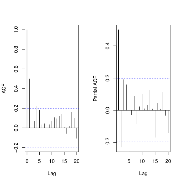
Figure 2: Autocorrelations and partial autocorrelations of the Annual Swedish fertility rates.

The real data set to be analysed refers to the Annual Swedish fertility rates (1000’s) from 1750 to 1849. These data are depicted in Figure 1 and were obtained from the website https://datamarket.com/data/set/22s2. Also, Figure 2 presents the sample autocorrelations and partial autocorrelations for the Annual Swedish fertility rates respectively.

In the first step, Bayesian selection criteria were used to compare between gamma and inverse Gaussian models and also to select the model order. The same criteria DIC, EBIC and CPO were employed and Table 4 presents the results. From this table we can see that the TGARMA(1,0) model with gamma distribution is preferred in terms of all the criteria although the TGARMA(1,1) with the same distribution is a close competitor. Table 5 presents the Bayesian estimates of the selected model with posterior means and standard deviations (in brackets), the 95% HPD intervals and acceptance rates from the Metropolis algorithm.

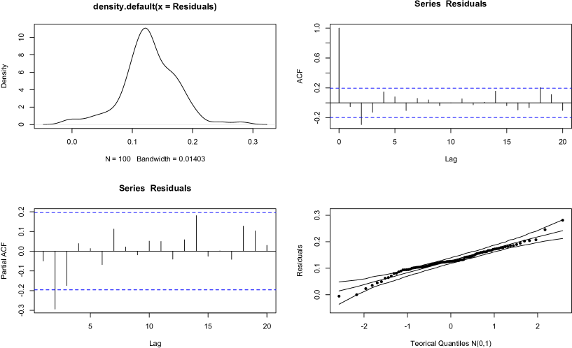
Figure 3: Autocorrelation function and partial autocorrelation function of the residuals of the Annual Swedish fertility rates series.

Finally, a residual analysis was carried out to assess the adequability of the chosen model. Quantile residuals are based on the idea of inverting the estimated distribution function for each observation to obtain exactly standard normal residuals. This is accomplished by defining the residuals as $r_{t}=\Phi^{-1}(\textbf{F}_{y_{t}}(y_{t}|F_{t-1}))$ where $\textbf{F}_{y_{t}}$ represents the cumulative distribution function for the associated density funcion. Figure 3 confirms residuals following Gaussian distribution and non-correlated.

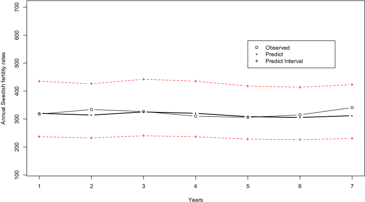
Figure 4: Predictions with TGARMA(1,0) Gamma model for the Annual Swedish fertility rates series.

The prediction were made by the median. Only the first term of Taylor expansion was used. Using the estimate, predictions of 6 steps ahead of the original series can be made. The 6 last values of the series were removed and fitted the model without them. Figure 4 presents predictions one step ahead for 6 years values, thus the predicted value be compared with the true value. The MAPE was calculated to assess the quality of predictions, the value was $03.70\%$ which indicated good predictions.

6 Discussion

In this paper we discussed a Bayesian approach for estimation, comparison and prediction of TGARMA time series models. We analyzed two different continuous models: gamma and inverse Gaussian. We implemented MCMC algorithms to carry out the simulation study and the methodology was also applied on a real time series dataset.

Properties of the Bayesian estimation and the performance of Bayesian selection criteria were also assessed with our simulation study. The analysis with real data also provided good estimates and predictions via parsimonious models. Our results suggest that, as indicated in the original TGARMA paper, this class of models has potential uses for modeling non-additivity, non-normality and heteroscedasticity continuous time series.

Table 1: Corrected bias (CB), corrected error (CE) and the mean acceptance rates (AP) for the TGARMA(1,1) model with gamma distribution and Box-Cox power transformation.

Parameter	True value	Mean	Variance	CB	CE	AP
$\lambda$	0.30	0.3025	0.0039	0.1504	0.9982	0.5939
$\nu$	0.50	0.5032	0.0011	0.0528	1.0023	0.7414
$\alpha_{0}$	0.70	0.6970	0.0277	0.1793	0.9976	0.6302
$\alpha_{1}$	0.50	0.4970	0.0019	0.0718	0.9996	0.5553
$\phi_{1}$	0.30	0.3008	0.0016	0.1036	0.9976	0.5863
$\lambda$	0.50	0.5052	0.0068	0.1266	1.0015	0.6771
$\nu$	0.50	0.5030	0.0010	0.0511	1.0040	0.7455
$\alpha_{0}$	0.70	0.7027	0.0281	0.1882	0.9996	0.6370
$\alpha_{1}$	0.50	0.4997	0.0018	0.0689	0.9995	0.5574
$\phi_{1}$	0.30	0.3008	0.0016	0.1069	1.0015	0.5854
$\lambda$	0.70	0.7095	0.0110	0.1208	1.0006	0.7276
$\nu$	0.50	0.5076	0.0013	0.0598	1.0182	0.7450
$\alpha_{0}$	0.70	0.7011	0.0316	0.2019	0.9964	0.6384
$\alpha_{1}$	0.50	0.4978	0.0019	0.0722	0.9976	0.5611
$\phi_{1}$	0.30	0.3008	0.0015	0.1096	0.9966	0.5873
$\lambda$	0.90	0.8783	0.0107	0.0969	1.0203	0.7634
$\nu$	0.50	0.5114	0.0010	0.0550	1.0581	0.7401
$\alpha_{0}$	0.70	0.6581	0.0217	0.1778	1.0382	0.6270
$\alpha_{1}$	0.50	0.4925	0.0018	0.0685	1.0140	0.5553
$\phi_{1}$	0.30	0.3020	0.0019	0.1147	0.9991	0.5831

Table 2: Proportions of correct model choice using Bayesian criteria with Gamma GARMA($p,q$) models.

	$\lambda=0.3$		$\lambda=0.5$
Model	GARMA(1,1)	GARMA(2,2)	GARMA(1,1)	GARMA(2,2)
EBIC	0.9820	0.4640	0.9920	0.4220
DIC	0.7900	0.7660	0.7940	0.7760
CPO	0.4260	0.7860	0.4300	0.8040

	$\lambda=0.7$		$\lambda=0.9$
Model	GARMA(1,1)	GARMA(2,2)	GARMA(1,1)	GARMA(2,2)
EBIC	0.9880	0.4900	0.9890	0.4540
DIC	0.8080	0.7860	0.7800	0.7510
CPO	0.4800	0.7800	0.4860	0.7950

Table 3: Corrected bias (CB), corrected error (CE) and the mean acceptance rates (AP) for the TGARMA(2,2) model with gamma distribution and Box-Cox power transformation.

Parameter	True value	Mean	Variance	CB	CE	AP
$\lambda$	0.30	0.3013	0.0010	0.0762	0.9971	0.3535
$\nu$	0.50	0.5060	0.0008	0.0474	1.0170	0.7407
$\alpha_{0}$	0.50	0.5332	0.0398	0.3074	1.0100	0.4085
$\alpha_{1}$	0.30	0.2790	0.0178	0.3406	1.0084	0.2771
$\alpha_{2}$	-0.20	-0.2064	0.0020	0.1810	1.0062	0.5685
$\phi_{1}$	0.40	0.4184	0.0182	0.2566	1.0055	0.2478
$\phi_{2}$	-0.30	-0.2788	0.0140	0.2956	1.0121	0.2421
$\lambda$	0.50	0.5031	0.0020	0.0654	0.9989	0.4252
$\nu$	0.50	0.5043	0.0009	0.0498	1.0063	0.7521
$\alpha_{0}$	0.50	0.5289	0.0380	0.3019	1.0076	0.4871
$\alpha_{1}$	0.30	0.2841	0.0169	0.3319	1.0040	0.3257
$\alpha_{2}$	-0.20	-0.2055	0.0020	0.1814	1.0042	0.5764
$\phi_{1}$	0.40	0.4139	0.0171	0.2461	1.0023	0.3301
$\phi_{2}$	-0.30	-0.2838	0.0133	0.2903	1.0064	0.3457
$\lambda$	0.70	0.7015	0.0036	0.0660	0.9961	0.5057
$\nu$	0.50	0.5064	0.0009	0.0501	1.0174	0.7378
$\alpha_{0}$	0.50	0.5321	0.0406	0.3102	1.0085	0.4414
$\alpha_{1}$	0.30	0.2822	0.0175	0.3347	1.0048	0.3271
$\alpha_{2}$	-0.20	-0.2076	0.0018	0.1732	1.0118	0.6342
$\phi_{1}$	0.40	0.4153	0.0173	0.2483	1.0026	0.2621
$\phi_{2}$	-0.30	-0.2813	0.0133	0.2905	1.0089	0.2928
$\lambda$	0.90	0.9025	0.0055	0.0642	0.9948	0.5932
$\nu$	0.50	0.5068	0.0009	0.0520	1.0177	0.7285
$\alpha_{0}$	0.50	0.5347	0.0442	0.3131	1.0079	0.5121
$\alpha_{1}$	0.30	0.2793	0.0156	0.3093	1.0075	0.2318
$\alpha_{2}$	-0.20	-0.2069	0.0016	0.1654	1.0087	0.5478
$\phi_{1}$	0.40	0.4191	0.0157	0.2304	1.0060	0.2114
$\phi_{2}$	-0.30	-0.2807	0.0126	0.2741	1.0089	0.2407

Table 4: Computed values of information criteria for the Annual Swedish fertility rates.

Gamma	TGARMA(1,0)	TGARMA(1,1)	TGARMA(1,2)	TGARMA(2,1)	TGARMA(2,2)
EBIC	1506.72	1507.51	1579.31	1544.57	1606.73
DIC	1496.66	1497.32	1570.84	1530.09	1596.48
CPO	-299.91	-300.76	-409.56	-306.09	-435.69
Inv. Gaussian	TGARMA(1,0)	TGARMA(1,1)	TGARMA(1,2)	TGARMA(2,1)	TGARMA(2,2)
EBIC	1664.14	1664.89	1683.51	1681.97	1686.55
DIC	1651.29	1652.56	1667.54	1665.44	1665.82
CPO	-336.96	-337.35	-381.22	-374.79	-392.01

Table 5: Estimates of Annual Swedish fertility rates series with TGARMA(1,0) Gamma.

Parameter	Mean (SD)	lower HPD limit	Upper HDP limit	AP
$\beta_{0}$	0.7888 (0.0537)	0.6497	0.9269	0.4928
$\phi_{1}$	0.7157 (0.0224)	0.6657	0.7650	0.4961
$\nu$	3.4782 (0.3516)	2.8195	4.1212	0.6701
$\lambda$	0.3145 (0.0326)	0.2513	0.3754	0.7382

Figure 1: Annual Swedish fertility rates from 1750 to 1849.

References

- Ahmad et al. (2015) Ahmad, W. M. A. W., Zakaria, S. B., Aleng, N. A., Halim, N. A., and Ali, Z. (2015). Box-Cox transformation and bootstrapping approach to one sample t-test. World Applied Sciences Journal, 33(5), 704–708.
- Benjamin et al. (2003) Benjamin, M., Rigby, R., and Stasinopoulos, D. (2003). Generalized autoregressive moving average models. . J. Amer. Statist. Assoc., 98, 214–223.
- Box and Cox (1964) Box, G. and Cox, D. (1964). An analysis of transformation. J. R. Statist. Soc. B, 26, 211–252.
- Castillo and F.G. (2013) Castillo, J. and F.G., B. (2013). Improving trip forecasting models by means of the Box–Cox transformation. Transportmetrica A: Transport Science, 9, 653–674.
- Cole et al. (2014) Cole, S. R., Chu, H., and Greenland, S. (2014). Maximum likelihood, profile likelihood, and penalized likelihood: a primer. American Journal of Epidemiology, 179(2), 252–260.
- Cox (1981) Cox, D. R. (1981). Statistical analysis of time series: Some recent developments. Scandinavian Journal of Statistics, 8, 93–115.
- da Silva et al. (2011) da Silva, M. V. G. B., Van Tassell, C. P., Sonstegard, T. S., Cobuci, J. A., and Gasbarre, L. C. (2011). Box-Cox transformation and random regression models for fecal egg count data. Frontiers in genetics, 2(00112).
- de Andrade et al. (2016a) de Andrade, B. S., Andrade, M. G., and Ehlers, R. S. (2016a). Bayesian GARMA models for count data. Communications in Statistics: Case Studies, Data Analysis and Applications, 1(4), 192–205.
- de Andrade et al. (2016b) de Andrade, B. S., Leśkow, J., and Andrade, M. G. (2016b). Transformed garma model: Properties and simulations. Communications in Statistics - Simulation and Computation.
- Draper and Cox (1969) Draper, N. R. and Cox, D. R. (1969). On distributions and their transformation to normality. J. R. Statist. Soc. B, 31, 472–476.
- Geweke (1992) Geweke, J. (1992). Evaluating the accuracy of sampling-based approaches to the calculation of posterior moments. In J. M. Bernardo, A. F. M. Smith, A. P. Dawid, and J. O. Berger, editors, Bayesian Statistics 4, pages 169–193. New York: Oxford University Press.
- Gillard (2012) Gillard, J. (2012). A generalised Box–Cox transformation for the parametric estimation of clinical reference intervals. Journal of Applied Statistics, 39, 2231–2245.
- Hamasaki and Kim (2007) Hamasaki, T. and Kim, S. (2007). Box and Cox power-transformation to confined and censored nonnormal responses in regression. Computational Statistics and Data Analysis, 51, 3788 – 3799.
- Huang et al. (2013) Huang, Z., Pang, Z., and Zhang, R. (2013). Adaptive profile-empirical-likelihood inferences for generalized single-index models. Computational Statistics and Data Analysis, 62, 70–82.
- Manly (1976) Manly, B. (1976). Exponential data transformation. The Statistician, 25, 37–42.
- R Development Core Team (2010) R Development Core Team (2010). R: A language and environment for statistical computing. R Foundation for Statistical Computing, Vienna, Austria.
- Sakia (1992) Sakia, R. (1992). The Box-Cox transformation technique: a review. The Statistician, 41, 168–178.
- Zhu and Ghodsi (2006) Zhu, M. and Ghodsi, A. (2006). Automatic dimensionality selection from the scree plot via the use of profile likelihood. Computational Statistics and Data Analysis, 51, 918–930.