Massively Parallel Computation of Accurate Densities for N–body Dark Matter Simulations using the Phase-Space-Element Method

Abstract

This paper presents an accurate density computation approach for large dark matter simulations, based on a recently introduced phase-space tessellation technique and designed for massively parallel, heterogeneous cluster architectures.

We discuss a memory efficient construction of an oct-tree structure to sample the mass densities with locally adaptive resolution, according to the features of the underlying tetrahedral tessellation. We propose an efficient GPU implementation for the computationally intensive operation of intersecting the tetrahedra with the cubical cells of the deposit grid, that achieves a speedup of almost an order of magnitude compared to an optimized CPU version. We discuss two dynamic load balancing schemes - the first exchanges particle data between cluster nodes and deposits all tetrahedra for each block of the grid structure on single nodes, whereas the second approach uses global reduction operations to obtain the total masses. We demonstrate the scalability of our algorithms for up to $256$ GPUs and TB–sized simulation snapshots, resulting in tessellations with over $400$ billion tetrahedra.

1 Motivation

Dark matter is a key component in state–of–the–art large–scale structure formation theories, and N–body simulations have become an essential method to test their predictions. This numerical approach treats dark matter as a collisionless gas, that is sampled by a set of particles of equal mass, whose positions are updated over time, according to the overall gravitational forces [1, 2, 3, 4, 5, 6, 7, 8, 9, 10, 11].

An integral part of N–body simulations, as well as applications that rely on an analysis of the resulting datasets, is the computation of accurate mass densities, for example, to solve the Poisson equation, identify features of the cosmic web or to predict dark matter annihilation signals. There exist various techniques to extrapolate from the mass at the discrete particle positions to a density field defined everywhere in the computational domain. Particles Mesh codes, for example, construct the underlying density field at the vertices, respectively cells of an auxiliary grid structure. The simplest technique, also known as Nearest Grid Point (NGP) [12], assigns the mass associated with each particle to the grid cell that contains it. The Cloud-In-Cell [13] approach models the particle’s mass distribution as a cube centered at its position and distributes the mass proportionally to all overlapping cells of a regular grid. Smoothed-Particle Hydrodynamics (SPH) schemes superimpose rotationally symmetric kernel functions centered at the particles [14]. Another technique is to construct Voronoi tessellations from the particles’ positions, estimating the densities using the particles’ enclosing volumes [15]. However, all these methods are subject to artifacts due to sampling noise inherent to the underlying discrete distributions, which is problematic in many applications.

In 2012, a density computation method for N–body simulations, not affected by the above-mentioned Poisson noise, was introduced [16, 17]. The basic idea is to use the tracer particles to construct a tessellation of the 3-dimensional dark matter sheet, which is embedded in a 6-dimensional phase space. Hereby the mass is spread out across the elements of the tessellation. Projecting the tessellation into configuration space and adding the density contributions from all elements that overlap the same spatial location, gives rise to well–defined densities in the entire computational domain.

This method has been successfully applied to reduce artificial clumping in N­-body simulations [18], to improve the quality of visualizations of dark matter simulations [19, 20], to create smooth maps of the gravitational lensing potential around dark matter halos [21], and to study the statistics of cosmic velocity fields [22]. It also led to the construction of new numerical schemes for dark matter simulations [23], and inspired work in computational geometry [24].

A drawback of the phase-space tessellation approach is its computational complexity, resulting from the large amount of tessellation elements that need to be processed. Fortunately, the inherently parallel nature of the problem is well–suited for massively parallel, heterogeneous cluster architectures equipped with accelerators, which recently have become very popular, because of their good performance and energy efficiency.

This paper presents a phase-space tessellation-based density computation approach for large N–body dark matter simulation data, utilizing massively parallel (GPU-)clusters. We introduce an exact tetrahedron–cube intersection algorithm, with optimized CPU and GPU variants, to sample the mass associated with the tetrahedral elements onto a block-structured grid.

The resolution of the grid is locally refined, based on the features of the underlying tessellation. Crucial for the overall performance is an efficient load balancing scheme, that distributes the workload equally across the cluster, while minimizing data transfers and memory requirements. We further compare two dynamic load-balancing strategies - one that gathers all tetrahedra required for depositing the mass onto each oct-tree patch on a single cluster node, as opposed to deposting only local tetrahedra, followed by a reduction step to obtain the total masses. We end the paper with a detailed analysis of the algorithm for various datasets of up to, including several weak and strong scaling tests.

2 Review of the Phase-Space Element Approach

In this section, we briefly review the main ideas of the phase-space tessellation method, that are most relevant for this paper – for a detailed discussion please refer to [16, 17]. N–body simulations model the large-scale evolution of dark matter in the Universe using point-like mass sources, called tracer particles or just tracers in the following discussion. Their positions are updated according to the aggregate gravitational forces, under the assumption, that the mass is centered at the tracers’ positions. However, it is physically more accurate to regard dark matter as a collisionless fluid, governed by the Vlasov-Poisson equation [25], with the mass spread out across the computational domain, instead of being concentrated at a number of quite arbitrary discrete sampling locations, as illustrated in the 2-dimensional phase-space diagram in Figure 1.

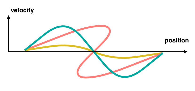
Figure 1: This 2D phase-space diagram shows the positions and velocities of the dark matter fluid for three different time-steps. Initially, the dark matter is almost uniformly distributed and at rest (yellow). Gravity accelerates the fluid elements which gain velocity (green) and at later times, several streams of the dark matter co-exist at the same spatial regions (red).

At the initial time step, the tracers are distributed almost uniformly throughout the computational domain, by aligning their positions with the vertices of a regular grid. We will refer to this arrangement as the Lagrangian grid in what follows.

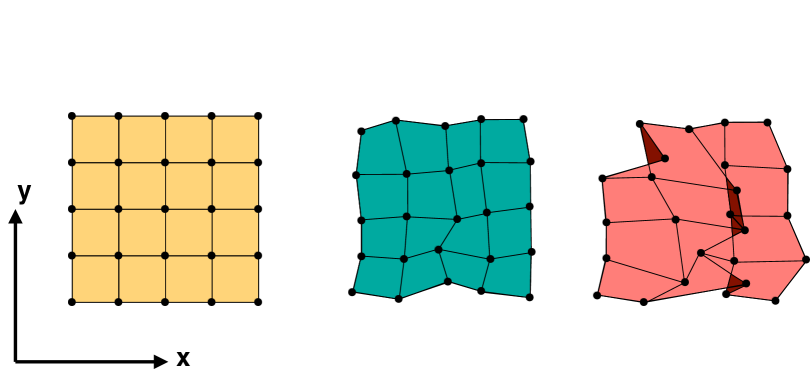
Figure 2: A 2D regular grid structure defined by the tracer particles of a N–body simulation. Initially, the particles are distributed regularly over the computational domain (left). Over time, the particles are advected due to gravitational forces and the cells become deformed (middle). At later times, cells finally start to overlap (dark shaded regions on the right).

Since each cell initially has the same volume and that the mass is distributed uniformly across the computational domain, the same mass is assigned to each cell. The cell connectivity is fixed over time, whereas the spatial locations of the vertices are updated according to the actual positions of the tracer particles, causing a deformation of the embedding of the logical rectangular Lagrangian grid in configuration space, as depicted in Figure 2. Given the constant mass per cell, its time-dependent volume provides an estimation of its local density. However, instead of directly using the hexahedral cells to compute these volumes, it is computational more efficient to first tessellate them by tetrahedra, as these are always convex, independently of the relative positions of their vertices. We will follow the tessellation choice using $6$ tetrahedra, as for example used in [19]. So if $m$ is the constant mass per tetrahedron and $\sum_{i}V_{i}(\mathbf{x},t)$ the total volume of all tetrahedra that cover the location $\mathbf{x}$ at time $t$, the total mass density is given by

$$\rho_{tot}(\mathbf{x},t)=m\sum_{i}\frac{1}{V_{i}(\mathbf{x},t)}.$$ (1)

3 Distributed Tessellation Construction

In this Section, we discuss the construction of the tetrahedral tessellation in a distributed environment. The goal is to assign approximately the same number of elements to each node, while exploiting as much spatial locality as possible, in order to reuse tracers that are shared between multiple elements. Our strategy it to subdivide the underlying logical Lagrangian grid into rectangular blocks, and assign them to different cluster nodes. To determine the three-dimensional layout of the blocks, we compute all possible factorizations of the number of nodes by three integers and choose the one that yields the most similar number of blocks along all dimensions. Tracer particles on common faces, edges and vertices between adjacent blocks are duplicated to ensure that each individual node has access to all data required to locally construct the tetrahedra associated with the cells of its block. The subdivision process is illustrated in Figure 3.

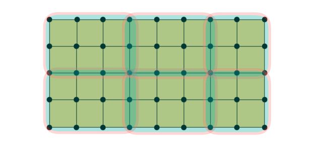
Figure 3: Example of the subdivision of a logical rectangular 2D Lagrangian grid with $9\times 5$ particles into 6 blocks, that are assigned to different cluster nodes. One layer of particles between adjacent blocks is duplicated to guarantee, that all tetrahedra can be reconstructed locally.

Large-scale N–body simulation codes usually store their data in spatially clustered arrangments, for example employing space-filling Hilbert-curves [5] or Morton-order layouts [9]. So that the data is already partially organized in blocks in Lagrangian grid space, in particular for the earlier time-steps, and since the tracers typically travel a relatively small fraction of the overall computational domain, the correlation between chunks of data on disk and blocks in Lagrangian grid space is partly conserved over time. So loading a chunk of contiguous data from file on each cluster node, and choosing a file offset that corresponds to the node’s assigned Lagrangian block, ensures that a large fraction of the loaded particle data is part of the node’s block. However, in general, a fraction of the tracers for each block will be unavailable, so internode communication will be required in order to exchange the missing data. We speed up this process by organizing the local particles into different bins, one for each block of the Lagrangian grid, respectively cluster node. The assignment to the bins is based on the particles’ Lagrangian positions, which is given by their unique IDs. Due to the shared boundary layers between adjacent Lagrangian blocks, a fraction of particles may be duplicated in up to $8$ bins. However, while this introduces only a small memory overhead, it avoids expensive search operations and allows to free entire bins efficiently, when the pairwise communication between pairs of nodes has been carried out. Once a node received all particle data for its local block, the tracers are sorted by their IDs, which then become obsolete and are discarded.

4 Constructing the Adaptive Grid Structure

In this section, we discuss the distributed construction of the adaptive deposit grid structure, an oct–tree, although an extension to more general structures like kD–, or AMR (adaptive mesh refinement) trees would be possible, too.

Starting at the root of the tree, which is defined by the minimal axis–aligned bounding box containing all tracer particles in the computational domain, all process detect the number of local tetrahedra that cover each node of the tree and obtains the overall number via a global reduction. If the number is above a user-defined threshold, the bounding box is refined by 8 children, and the process continues recursively, until the number of elements that partially overlap the node’s region is below the threshold or a minimal node extension is reached. The latter is necessary because the number of tetrahedra does not always decrease on the refined regions, for example, once it is completely contained inside the intersection of a set of tetrahedra. The leaf nodes of the tree are overlaid by cubical grid patches of the same number of cells and thus yield a sampling of the computational domain, whose local resolution is adapted to the density of the tetrahedra.

A drawback of the approach discussed so far is its high memory consumption. since in order to efficiently check the refinement criterion, one has to keep track of sets of local tetrahedra that cover different parts of the tree, e.g. by storing their unique IDs at each node of the tree. But the number of tetrahedral exceeds the number of tracer particles by a almost a factor of $6$, and at least $64$-bit integers are necessary to uniquely identify them, so even in the optimal case that each element falls into exactly one leaf node and thus needs to be stored only once, the memory requirements would exceed the one for storing the original tracer positions.

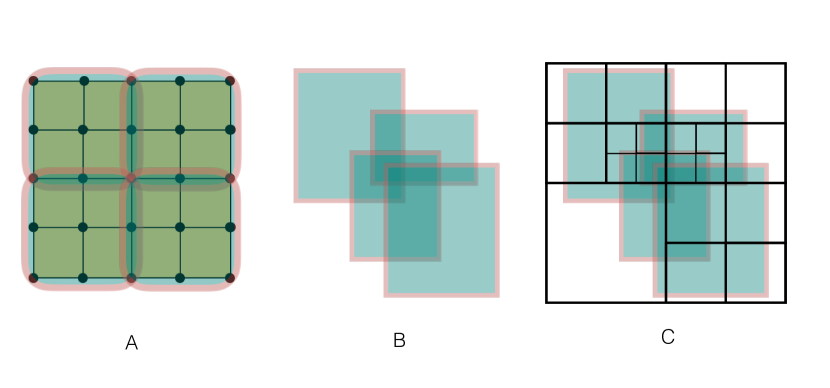
Figure 4: 2D illustration of a memory efficient oct-tree construction: (A) shows a Lagrangian grid block with $5\times 5$ particles, which is further subdivided into 4 subblocks. (B) The minimal axis-aligned bounding boxes, spanned by the particles of each of these subblocks, in configuration space. (C) The quad-tree (oct-tree) structure, refined based on the area (volume) of covered subblocks.

In order to reduce this overhead, we further partition the local Lagrangian grid block on each node of the cluster into a set of subregions, called subblocks in the following discussion, and precompute the partially overlapping, minimal axis-aligned bounding boxes enclosing the particles of each subblock. Instead of testing each tetrahedron individually, we base the refinement decision on the volume of the intersection between these bounding boxes and the tree nodes. The IDs of intersecting subblock are stored at each tree node, which drastically reduces the memory overhead in comparison to storing the IDs of individual tetrahedra. The number of tetrahedra that overlap a specific tree node is estimated by the intersection volume between the nodes and the subblocks’ bounding boxes, assuming that the tetrahedra in each subblock have similar volumes. A number $8^{3}$ cells for each subblock worked well for our applications, in terms of the trade-off between the number of generated subblocks and the spatial locality of the tetrahedra. A overview of the oct-tree construction is given in Figure 4.

5 Dynamic Load Balancing

In general, the tetrahedra density will vary substantially across the computational domain, ranging from a few elements per point in underdense voids, to several thousand in dark matter halos. To some extent, we account for this variance by adapting the spatial resolution of the oct-tree to the density of the underlying tessellation. However, the workload still differs for the leaf nodes of the tree, so an efficient load-balancing technique is crucial for optimally utilizing the computational resources.

We employ dynamic load balancing strategies on three different levels: between individual compute nodes, between individual CPU threads on each compute node, as well as on the level of GPU kernel calls, launched by the CPU threads. The latter two will be discussed in detail in Section 6, while here we focus on load balancing the compute nodes.

In general, the tetrahedra required for depositing the mass onto a leaf node of the tree structure will be scattered across multiple compute nodes and we will discuss two options for processing each leaf: (A), gathering all required tetrahedra on one compute node, which deposits the elements’ masses, or alternatively (B), depositing only the local tetrahedra on each compute node, followed by a reduction operation between all processes that contributed to the leaf. In the next two paragraphs, we will describe our implementations of these approaches using MPI, and defer a performance comparison between them to Section 7. In both cases, we launch one MPI process per compute node and at least two CPU threads per MPI rank, in order to overlap local computation and internode communication.

Option (A): Exchanging Point Data

In this approach, each MPI rank enters a loop and signals all other ranks if it is ready for new work, by setting a flag in a bitmask, one bit for each rank, that is globally reduced. The first rank R that is ready for new work, is assigned the leaf node L, for which it locally stores most of the required tetrahedra. The other MPI ranks send their local tetrahedra that overlap L, to R, which starts depositing the elements, as discussed in detail in Section 6, while, concurrently, new work is assigned to other MPI ranks. Instead of constructing the tetrahedra of the Lagrangian blocks before sending them to the target rank, each compute node sends complete $8^{3}$ subblocks of particles and R constructs the tessellation elements locally, thereby drastically reducing the amount of transferred data. The overall algorithm is outlined in the pseudo-code in Figure 5.

1:  launch local worker threads

2:  leafNodeList $\leftarrow$ all octree leaf nodes

3:  while  leafNodeList NOT empty  do

4:     if  local worker threads finished  then

5:        store mass of previous grid patch

6:     end if

7:     MPI: share which processes are ready for new work

8:     for all  processes R that are ready for new work  do

9:        L $\leftarrow$ FindBestOctreeLeafNode( R, leafNodeList )

10:        remove L from leafNodeList

11:        MPI: subblocks that overlap L are send to R

12:        if  this rank == R  then

13:           local worker threads start mass deposit for L

14:        end if

15:     end for

16:  end while

Figure 5: Pseudo code for communication approach (A) on each MPI process. Lines beginning with ’MPI:’ indicate points of internode communication.

Option (B): Global Reduction

In this approach, each MPI process enters a loop, picks the next leaf node for which it has local tetrahedra and starts the mass deposit using its set of worker threads, see Section 6. Concurrently, the MPI ranks reduce a bit mask that indicates which of the leaves are finished on each node. Once the mass deposit for a leaf has been completed on all cluster nodes, the masses of the local mass arrays are combined to yield the resulting densities. This is achieved via a global reduction operation between all ranks that contributed mass to the leaf node. The reduction’s target rank is altered in a round-robin fashion, in order to distribute the workload.

1:  launch local worker threads

2:  leafNodeList $\leftarrow$ all octree leaf nodes

3:  allocate buffer B (stores octree leaf masses)

4:  repeat

5:     if  local worker threads finished work item  then

6:        B $\leftarrow$ local mass of processed octree leaf

7:     end if

8:     if $($ B NOT full $)$ AND $($ leafNodeList NOT empty $)$ then

9:        L $\leftarrow$ next leaf node in leafNodeList

10:        remove L from leafNodeList

11:        local worker threads start mass deposit for L

12:     end if

13:     MPI: determine which leaves are globally finished

14:     for all newly finished octree leaves L do

15:        if  this rank contributed mass to L  then

16:           R $\leftarrow$ process that stores final grid patch mass

17:           MPI: total masses for L via reduction to R

18:           if  this rank == R then

19:              store total masses for L

20:           end if

21:           remove L from buffer B

22:        end if

23:     end for

24:  until  all leaf node masses have been stored

Figure 6: Pseudo code for communication approach (B), executed on each MPI process. Lines beginning with ’MPI:’ indicate interprocess communication points.

In case the mass deposit is completed locally but not globally, the corresponding local mass array is buffered, and the next leaf is processed, in order to avoid that the worker threads idle. However, once the buffer’s maximal storage capacity is reached, the rank has to postpone the deposit of new blocks, until at least one of its buffered leaf nodes is finished on all nodes. The algorithm is outlined in Figure 6.

6 Mass Deposit

As discussed in the last Section, concurrent computation and communication is enabled by launching several threads per MPI process: one communication thread, the main thread, for data exchange between cluster nodes, as well as at least one worker thread to manage the deposition of the tetrahedra masses. Here we will give an overview of the multi-threaded mass deposit approach and defer the CPU and GPU specific implementation details to the next Subsections.

In both cases, the worker threads keep running until all oct-tree leaf nodes have been processed. The Lagrangian subblocks, see Section 3, that overlap the spatial extent of the current leaf node, are distributed to the available worker threads. We found that splitting them into 10 times more groups, than the number of worker threads, leads to good results in terms of dynamic load balancing between the worker threads. Each thread allocates its own private memory buffer to accumulate the mass contributions. The mass deposit step involves the computation of the exact intersection volumes between the tetrahedra and the cubical grid cells and will be discussed in detail in the Subsection 6.3. Once a worker thread has deposited all mass associated with its tetrahedra, it is assigned the next set of Lagrangian cell blocks and once all blocks have been processed, the separate private mass buffers are added and the worker threads signal the main thread that they are ready for new work.

6.1 CPU Implementation

In the CPU case, each worker thread operates on one cell $L$ of its assigned Lagrangian grid blocks at a time. Its minimal, axis-aligned bounding box is constructed and tested for intersection with the extent of the leaf node’s deposit grid patch. In the case of no intersection, L’s 6 tetrahedra are skipped and the next cell is processed. Otherwise the first of the $6$ tetrahedra, $T_{0}$, is constructed, its minimal bounding box is determined and the worker thread loops over all cells $C_{i}$ of the deposit grid patch that overlap the bounding box of $T_{0}$. For each cell $C_{i}$, we first test for trivial intersection configurations between $C_{i}$ and $T_{0}$, i. e. no intersection, $C_{i}$ completely inside $T_{0}$ or vice versa, which is implemented by computing the relative orientation of the vertices of $T_{0}$ with respect to the axis-aligned faces of $C_{i}$. Otherwise, the computationally more intensive algorithm discussed in Subsection 6.3 is used to compute the exact intersection volume. The resulting volume is transformed to its mass equivalent, stored in the thread’s private memory location for cell $C_{i}$ and the next tetrahedron of $L$ is processed.

6.2 GPU Implementation

In the GPU case, we start one CPU thread for each available local GPU and keep it running, until all leaf nodes of the grid structure have been processed. Each CPU thread allocates private GPU memory to store the Lagrangian grid block as well as a buffer to accumulate the mass contributions.

On GPU achitectures, code divergence can severely degrade overall performance, since sets of threads operate in lock-step and different code paths causes subsets of the GPU threads to idle, resulting in an underutilization of the available computational resources. This poses a challenge for the geometry intersection, since the amount of work for the tetrahedra differs substantially, depending, for example, on how many deposit cells are covered and on the number of non-trivial intersection configurations.

On current NVIDIA GPU architectures, sets of 32 threads, called lanes, form a warp and operate in lock-step. Hence, assigning one tetrahedron to each lane, can result in only one of 32 threads performing useful work. One potential solution would be to use different GPU kernels, one that classifies the type of intersections and buffers the results in global GPU memory, as well as two separate kernels that process the trivial and non-trivial intersection cases, similar to the techniques discussed for 2D triangle rasterization in CUDA raster [26]. However, in the 3-dimensional case, this would quickly exceed the available global GPU memory due to the drastically larger number of cells in the 3D deposit grids, as compared to the 2-dimensional framebuffers, as well as the sheer size of the tesselations our approach targets.

We therefore follow a different approach, that avoids the usage of additional global memory by processing one tetrahedron per warp, using a single GPU kernel. Each warp picks a separate Lagrangian cell, tests its bounding box for intersection with the oct–tree node and, in case of an intersection, constructs the first of the $6$ tetrahedra. Each lane picks a different cell of the deposit grid patch and classifies the intersection configuration in lock-step. Since the trivial cases are not computationally expensive and cause only minimal thread divergence, they are processed immediately, using an atomic operation to update the GPU’s global memory entry for this cell. However, in case a lane detects a non-trivial configuration, the more expensive intersection routine discussed in Subsection 6.3 is not called immediately. Instead the cell’s ID is stored in the fast, low-latency shared memory, as depicted using the 2D example in Figure 7. We use a buffer size of $64$ single precision integers, and determine the current buffer position for each lane using an atomic counter in shared memory. The lanes continue to classify cells, until the number of IDs, stored in the shared memory buffer, exceeds $31$. In this case, each lanes picks one buffered ID and calls the exact intersection routine for its cell. Once all lanes in the warp returned from the call, they classify the next set of 32 cells in lock-step. For our test cases, this approach reduced thread divergence substantially and performed about $20$ times faster compared to an alternative “one-tetrahedron per GPU thread” approach.

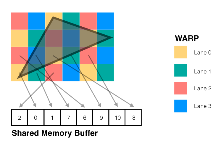
Figure 7: 2D example of the GPU rasterization approach for a hypothetical warp size of 4. The lanes in the warp, depicted by different colors, classify 4 cells in lock-step. The IDs of cells intersecting the edges of the triangle are stored in a buffer in shared memory and processed in lock-step in a separate step.

6.3 Tetrahedron-Cube Intersection

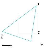
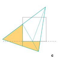
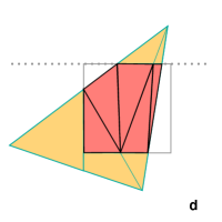
Figure 8: Computing the area of the intersection between cell $C$ and triangle $T$, by iteratively splitting $T$ against lines defined by the edges of $C$, followed by a triangulation of the resulting polygon on the half-space that includes $C$.

In this Subsection, we describe our algorithm for computing the volume of the intersection between a tetrahedron $T$ and a cubical cell $C$. For the sake of simplicity, we explain the algorithm in 2D, since the generalization to 3D is straightforward. So the task is to compute the area of the intersection between a triangle $T$ and the quadratic cell $C$. Let us assume that the cell’s lower left vertex is at $(x=0,y=0)$ and its upper right at $(x=1,y=1)$, as depicted in Figure 8 (a).

The first step is to intersect $T$ with the line defined by $(x=0,y)$. If the entire triangle is located on the half-plane defined by $(x\leq 0,y)$, the intersection volume is zero and the algorithm terminates. Otherwise the resulting polygon, located on the half-plane $(x>0,y)$ that includes $C$, is triangulated by up to two triangles, as shown in Figure 8 (b). Next, the newly generated triangles are tested for intersection with the line $(x,y=0)$, the resulting interior region is triangulated and the procedure is repeated for the lines $(x=1,y)$ and $(x,y=1)$. The intersection area is computed by summing the areas of the resulting triangles. The approach operates analogously in $3$-dimensions, where the tetrahedron is iteratively split against the 2D planes defined by the faces of the cell. In order to speed up the triangulation of auxiliary polygons, we precompute all different cases and store them in a look-up table. The location of the vertices of $T$ relative to each plane defines a bitmask that serves as a lookup index into the table, which returns the number of resulting tetrahedra as well as the connectivity information to construct the intermediate geometry. Instead of carrying out the algorithm as sketched above for all three dimensions, for the third dimension, we triangulate the parts of the polygons outside $C$’s halfspace, instead the one inside, and subtract its volume from the interior tetrahedra, since this generally reduces the amount of generated geometry.

A possible GPU implementation is to cache the intermediate tetrahedra and reuse them for each new dimension that is processed. However, on the GPU, the fast shared memory is too small to store all geometry, so it would have to be moved to slower global memory, substantially degrading overall performance. Therefore, we avoid to cache intermediate tetrahedra and prune each tetrahedron separately against all cell’s faces, before the next intermediate tetrahedron is processed. Although this involves redundant computations, it turns out to increase performance on massively parallel graphics hardware, where data movement is relatively expensive compared to computation.

7 Results and Discussions

We conducted our experiments on the Sherlock and XStream HPC clusters at the Stanford Research Computing Center (SRCC). Sherlock’s hardware resources include 120 general compute nodes, each with a dual socket Intel Xeon CPU E5-2650 v2 at $2.60$ GHz, 8 cores per socket and $64$ GB DDR3 RAM. XStream consists of 65 compute nodes, each equipped with 2 x Intel Xeon CPU E5-2680 v2 @ 2.80GHz (10 cores per socket), 256 GB of RAM and 8 x NVIDIA Tesla K80 (16 logical GPUs). Both clusters are interconnected with FDR Infiniband and have access to a PB sized Lustre parallel file system. For our measurements we used simulation snapshots with $2048^{3}$ and $4096^{3}$ particles at redshift $0$ from the Dark Sky Simulations: Early Data Release [27].

7.1 Strong Scaling

The strong scaling tests utilized between $128$ and $2048$ CPU cores on Sherlock, with one MPI rank per compute node and $8$ threads per MPI rank. The test problem was the exact mass deposit of a $2048^{3}$ particles N–body simulation onto a fully refined octree with 4 levels of refinement and $128^{3}$ cells per node, resulting in a total grid resolution of $2048^{3}$ cells. Tables 9 and 10 as well as Figure 11 summarize the results for the two different communication strategies discussed in Section 5 - exchanging point data A versus exchanging deposit grid arrays between cluster nodes B. .

For approach B, up to $5000$ leaf node mass arrays per compute node were locally cached on each process. As shown in tables 9 and 10, the performance of approach A was between $1.2$ and $1.9$ times faster. Also in terms of scalability, approach A, which shows almost perfect scaling up to $1024$ cores, outperformed B. For $2048$ cores, the speed-up was reduced from a theoretical factor of 16 to about 11, due to increased overhead of communication between the cluster nodes.

# CPU cores	Time (min)	Speedup
128	603	1.0
256	331	1.8
512	143	4.2
1024	81	7.4
2048	53	11.2

Figure 9: Strong scaling results for communication strategy A for depositing the mass associated with a $2048^{3}$ particles N–body simulation onto a fully refined octree with 4 levels of refinement and $128^{3}$ cells per node, resulting in a total grid resolution of $2048^{3}$ cells.

# cores	Time (min)	Speedup
128	712	1.0
256	458	1.6
512	266	2.7
1024	129	5.0
2048	77	9.2

Figure 10: Strong scaling results for communication alternative B, using the same test problem as in Table 9.

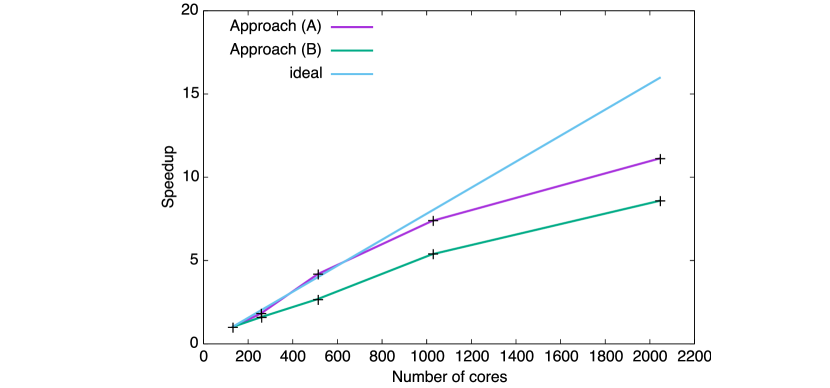
Figure 11: Strong scaling results for $2048^{3}$ particles.

7.2 Weak Scaling

In order to ensure that the complexity of the workload for the different datasets used for the weak scaling test scales linearly with the number of utilized cores, the different datasets were generated analytically, by placing the dark matter particles onto a uniform grid and adding randomized positive or negative offsets of up to one cell width in each direction to the particle positions. The number of particles and the number of cells in the deposit grid was successively increased by a factor of two, ranging from $512^{3}$ to $2048^{3}$ particles, with $256^{3}$ to $1024^{3}$ cells in the deposit grid structure. The datasets were processed utilizing between $32$ and $2048$ cores on $1$ up to $64$ nodes on the Sherlock cluster, doubling the number of nodes between consecutive tasks. The resulting wall clock times for communication strategy (A) are given in Figure 12.

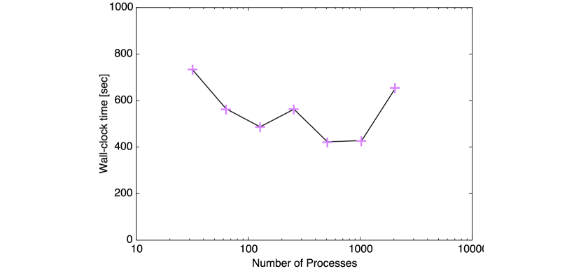
Figure 12: Weak scaling results for a mass deposit problem using $512^{3}$ to $2048^{3}$ particles, using between $32$ and $2048$ processes.

7.3 GPU Performance

The performance between the CPU and GPU version of the code discussed in Section 6, was conducted on one node of the XStream GPU cluster, with two Intel Xeon Processor E5-2680 v2 CPUs and one Nvidia K80 card with two Kepler GK210 GPUs. The peak performance for the CPU version was achieved with $40$ threads ($2$ cores with hyperthreading). The test problem was the mass deposit for a N–body simulation with $2048^{3}$ particles onto a fully refined octree with 4 levels of refinement and $128^{3}$ cells per node, resulting in a total grid resolution of $2048^{3}$ cells. The CPU version took about $1995$ minutes to complete, whereas the GPU version was finished in about $230$ minutes, so the achieved GPU speedup was about $8.7$. Figure 14 and Table 13 show the result of a strong scaling test on a single node of the XStream cluster, utilizing between $1$ and all $16$ available GPUs. The test dataset was a $1024^{3}$ particle dataset. The speedup increased roughly linearly with the number of GPUs with a slope of about $0.63$, due to the increased overhead of transferring the point data from the CPU to several GPUs and reducing the local deposit grid arrays back on the CPU.

# GPUs	Time (sec)	Speedup
1	4144	1.0
2	2170	1.9
3	1556	2.7
4	1217	3.4
5	1035	4.0
6	877	4.7
7	780	5.3
8	720	5.8
9	655	6.3
10	582	7.1
11	534	7.8
12	481	8.6
13	486	8.5
14	447	9.3
15	452	9.2
16	422	9.8

Figure 13: Strong scaling results for up to 16 GPUs.

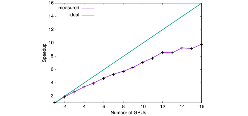
Figure 14: Ideal and measured GPU strong scaling results for $1024^{3}$ particles and $1$ to $16$ GPUs.

We further performed an adaptive mass deposit test using a $4096^{3}$ particle N–body dataset, using a leaf node size of $64^{3}$ cells per node and a maximum of $7$ refinement levels, resulting in an effective resolution of $8192^{3}$ cells on the highest level of resolution. The test was run on 16 compute nodes of XStream, utilized all available 8 Nvidia K80 cards per node and finished in $46$ minutes. Figure 15 shows a visualization of the multi-resolution density field with direct volume rendering.

8 Summary and Future Work

We presented an approach for the distributed computation of accurate density fields from large N–body dark matter simulations, using the phase-space element technique, that is tailored to massively parallel cluster architectures equipped with GPU accelerators. We employed an oct-tree grid structure to sample the densities onto cubical cells, adapting the resolution according to the features of the underlying tessellation. We introduced a GPU algorithm for the computationally intensive step of geometrically intersecting the tetrahedra with the cubical cells of the octree, which achieves almost an order of magnitude speedup compared to an optimized CPU implementation. We further presented two dynamic load balancing strategies and demonstrated the overall good weak and strong scaling performance of our approach with several large datasets. Our measurements showed that it is beneficial to communicate particle data, instead of reducing deposit grid patches in terms of overall performance and scaling features.

We see various directions for future work. It would be interesting to compare the performance of the GPU implementation with one optimized for Intel Xeon Phi coprocessors. We would also like to investigate if the proposed solution can be extended and applied to in-situ scenarios, i.e., performed alongside the underlying simulation, by sharing the available hardware resources. Furthermore, in addition to the mass deposit onto the leafs nodes of the oct-tree structure, generating coarser representations for the internal nodes would be beneficial for interactive visualization approaches, like direct volume rendering, that employ multi-resolution representations of the data to achieve interactive frame rates. Our implementation is open source and available at https://github.com/kaehlerr/ADECO.

9 Acknowledgments

We are very grateful to Tom Abel and Devon Powell for useful discussions on this topic. We would also like to thank the Dark Sky Simulations collaboration for making their data publically available, in particular Sam Skillman for his advice regarding the data format. This work used the Sherlock and XStream clusters, hosted at the Stanford Research Computing Center, which is supported by the National Science Foundation Major Research Instrumentation program (ACI-1429830). We would also like to thank Nvidia for supporting KIPAC’s computing department with several GPUs.

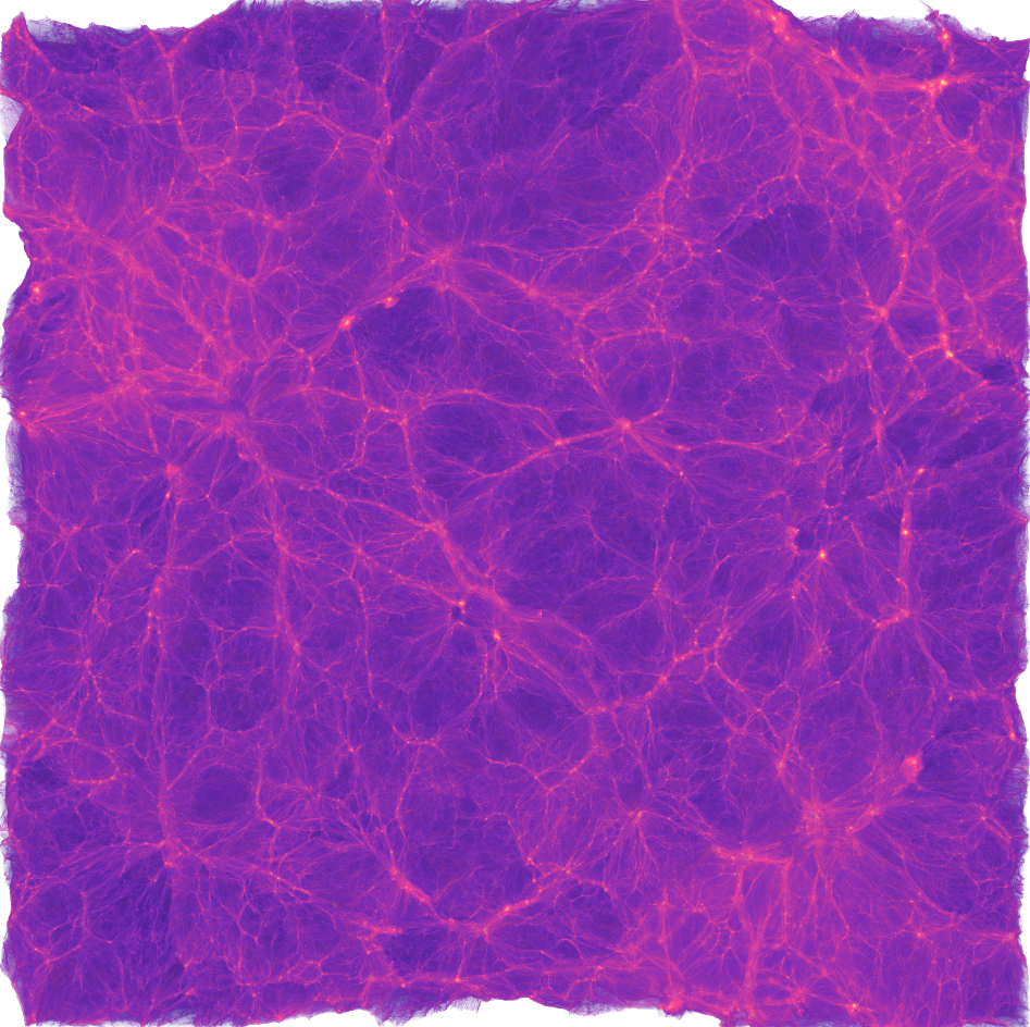
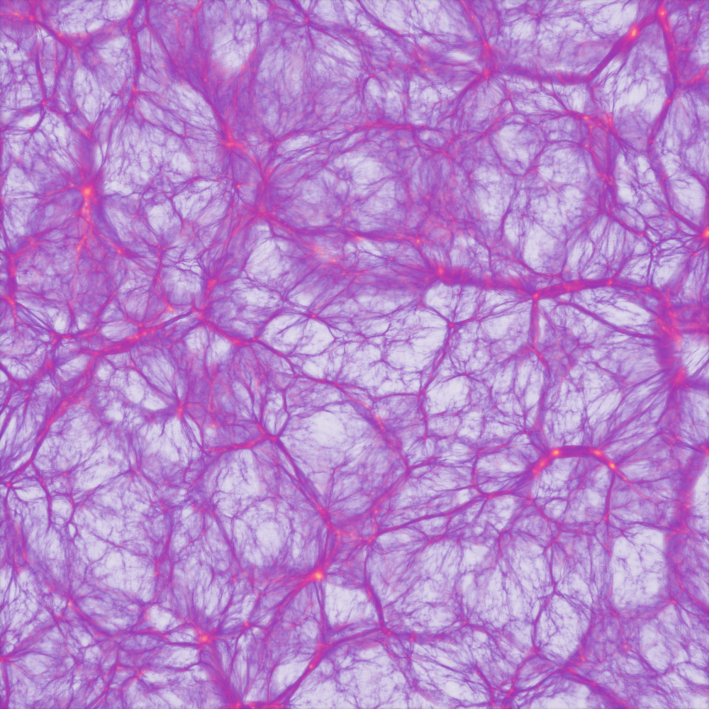
Figure 15: Direct volume rendering of a N–body simulation with $4096^{3}$ particles. The mass was resampled onto an oct-tree data structure with an effective resolution of $8192^{3}$ cells. The upper part shows the whole domain, whereas the lower one depicts a zoomed view of a thin slice through the volume.

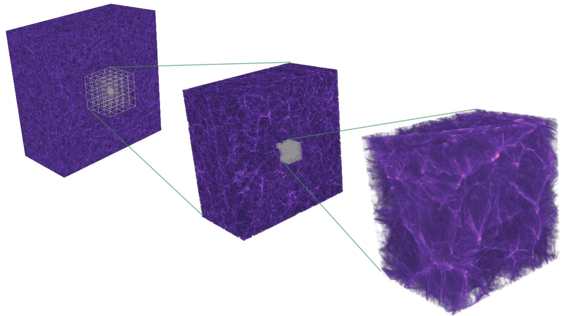
Figure 16: Direct volume rendering of a N–body simulation with $4096^{3}$ particles, zooming from a region of $1600$ Mpc down to a region of about $6$ Mpc. The mass was resampled onto an oct-tree data structure with $9$ levels of resolution.

References

-
[1]
M. D. Dikaiakos, J. Stadel, A
performance study of cosmological simulations on message-passing and
shared-memory multiprocessors, in: Proceedings of the 10th International
Conference on Supercomputing, ICS ’96, ACM, New York, NY, USA, 1996, pp.
94–101.
doi:10.1145/237578.237590.
URL http://doi.acm.org/10.1145/237578.237590 -
[2]
A. V. Kravtsov, A. A. Klypin, A. M. Khokhlov,
Adaptive refinement tree:
A new high-resolution n-body code for cosmological simulations, The
Astrophysical Journal Supplement Series 111 (1) (1997) 73.
URL http://stacks.iop.org/0067-0049/111/i=1/a=73 - [3] R. Teyssier, Cosmological hydrodynamics with adaptive mesh refinement: a new high resolution code called ramses, Astron. Astrophys. 385 (2002) 337–364. arXiv:astro-ph/0111367, doi:10.1051/0004-6361:20011817.
- [4] J. Dubinski, J. Kimb, C. Park, R. Humbleb, GOTPM: a parallel hybrid particle-mesh treecode, New Astronomy 9 (2004) 111–126. doi:10.1016/j.newast.2003.08.002.
- [5] V. Springel, The Cosmological Simulation Code Gadget-2, Monthly Notices of the Royal Astronomical Society 364.
-
[6]
M. Wetzstein, A. F. Nelson, T. Naab, A. Burkert,
Vine a numerical code
for simulating astrophysical systems using particles. i. description of the
physics and the numerical methods, The Astrophysical Journal Supplement
Series 184 (2) (2009) 298.
URL http://stacks.iop.org/0067-0049/184/i=2/a=298 -
[7]
T. Ishiyama, T. Fukushige, J. Makino, Greem: Massively parallel treepm
code for large cosmological n-body simulations, Publications of the
Astronomical Society of Japan 61 (6) (2009) 1319.
arXiv:/oup/backfile/content_public/journal/pasj/61/6/10.1093/pasj/61.6.1319/2/pasj61-1319.pdf,
doi:10.1093/pasj/61.6.1319.
URL +http://dx.doi.org/10.1093/pasj/61.6.1319 -
[8]
S. Habib, V. Morozov, N. Frontiere, H. Finkel, A. Pope, K. Heitmann,
Hacc: Extreme scaling and
performance across diverse architectures, in: Proceedings of the
International Conference on High Performance Computing, Networking, Storage
and Analysis, SC ’13, ACM, New York, NY, USA, 2013, pp. 6:1–6:10.
doi:10.1145/2503210.2504566.
URL http://doi.acm.org/10.1145/2503210.2504566 -
[9]
M. S. Warren, 2hot: An
improved parallel hashed oct-tree n-body algorithm for cosmological
simulation, in: Proceedings of the International Conference on High
Performance Computing, Networking, Storage and Analysis, SC ’13, ACM, New
York, NY, USA, 2013, pp. 72:1–72:12.
doi:10.1145/2503210.2503220.
URL http://doi.acm.org/10.1145/2503210.2503220 - [10] G. L. Bryan, M. L. Norman, B. W. O’Shea, T. Abel, J. H. Wise, M. J. Turk, D. R. Reynolds, D. C. Collins, P. Wang, S. W. Skillman, B. Smith, R. P. Harkness, J. Bordner, J.-h. Kim, M. Kuhlen, H. Xu, N. Goldbaum, C. Hummels, A. G. Kritsuk, E. Tasker, S. Skory, C. M. Simpson, O. Hahn, J. S. Oishi, G. C. So, F. Zhao, R. Cen, Y. Li, Enzo Collaboration, ENZO: An Adaptive Mesh Refinement Code for Astrophysics, apjs 211 (2014) 19. arXiv:1307.2265, doi:10.1088/0067-0049/211/2/19.
-
[11]
A. S. Almgren, J. B. Bell, M. J. Lijewski, Z. Luki , E. V. Andel,
Nyx: A massively parallel
amr code for computational cosmology, The Astrophysical Journal 765 (1)
(2013) 39.
URL http://stacks.iop.org/0004-637X/765/i=1/a=39 - [12] R. W. Hockney, J. W. Eastwood, Computer Simulation Using Particles, Taylor & Francis, Inc., Bristol, PA, USA, 1988.
- [13] C. K. Birdsall, D. Fuss, Clouds-in-clouds, clouds-in-cells physics for many-body plasma simulation, Journal of Computational Physics 3 (1969) 494–511. doi:10.1016/0021-9991(69)90058-8.
- [14] J. J. Monaghan, An introduction to SPH, Computer Physics Communications 48 (1988) 89–96. doi:10.1016/0010-4655(88)90026-4.
- [15] M. C. Neyrinck, ZOBOV: a parameter-free void-finding algorithm, mnras 386 (2008) 2101–2109. arXiv:0712.3049, doi:10.1111/j.1365-2966.2008.13180.x.
-
[16]
S. Shandarin, S. Habib, K. Heitmann,
Cosmic web,
multistream flows, and tessellations, Phys. Rev. D 85 (2012) 083005.
doi:10.1103/PhysRevD.85.083005.
URL http://link.aps.org/doi/10.1103/PhysRevD.85.083005 -
[17]
T. Abel, O. Hahn, R. Kaehler,
Tracing the
dark matter sheet in phase space, Monthly Notices of the Royal Astronomical
Society 427 (1) (2012) 61–76.
arXiv:http://mnras.oxfordjournals.org/content/427/1/61.full.pdf+html,
doi:10.1111/j.1365-2966.2012.21754.x.
URL http://mnras.oxfordjournals.org/content/427/1/61.abstract - [18] O. Hahn, T. Abel, R. Kaehler, A new approach to simulating collisionless dark matter fluids, Mon. Not. Roy. Astron. Soc. 434 (2013) 1171. arXiv:1210.6652, doi:10.1093/mnras/stt1061.
- [19] R. Kaehler, O. Hahn, T. Abel, A novel approach to visualizing dark matter simulations, IEEE Transactions on Visualization and Computer Graphics 18 (12) (2012) 2078–2087. doi:doi.ieeecomputersociety.org/10.1109/TVCG.2012.187.
-
[20]
O. Igouchkine, N. Leaf, K.-L. Ma,
Volume rendering dark
matter simulations using cell projection and order-independent transparency,
in: SIGGRAPH ASIA 2016 Symposium on Visualization, SA ’16, ACM, New York, NY,
USA, 2016, pp. 8:1–8:8.
doi:10.1145/3002151.3002163.
URL http://doi.acm.org/10.1145/3002151.3002163 - [21] R. E. Angulo, R. Chen, S. Hilbert, T. Abel, Towards noiseless gravitational lensing simulations, Mon. Not. Roy. Astron. Soc. 444 (3) (2014) 2925–2937. arXiv:1309.1161, doi:10.1093/mnras/stu1608.
- [22] O. Hahn, R. E. Angulo, T. Abel, The Properties of Cosmic Velocity Fields, Mon. Not. Roy. Astron. Soc. 454 (4) (2015) 3920–3937. arXiv:1404.2280, doi:10.1093/mnras/stv2179.
- [23] O. Hahn, R. E. Angulo, An adaptively refined phase space element method for cosmological simulations and collisionless dynamics, Mon. Not. Roy. Astron. Soc. 455 (1) (2016) 1115–1133. arXiv:1501.01959, doi:10.1093/mnras/stv2304.
- [24] D. Powell, T. Abel, An exact general remeshing scheme applied to physically conservative voxelization, J. Comput. Phys. 297 (2015) 340–356. arXiv:1412.4941, doi:10.1016/j.jcp.2015.05.022.
- [25] P. J. E. Peebles, Principles of Physical Cosmology, 1993.
-
[26]
S. Laine, T. Karras,
High-performance software
rasterization on gpus, in: Proceedings of the ACM SIGGRAPH Symposium on High
Performance Graphics, HPG ’11, ACM, New York, NY, USA, 2011, pp. 79–88.
doi:10.1145/2018323.2018337.
URL http://doi.acm.org/10.1145/2018323.2018337 - [27] S. W. Skillman, M. S. Warren, M. J. Turk, R. H. Wechsler, D. E. Holz, P. M. Sutter, Dark Sky Simulations: Early Data ReleasearXiv:1407.2600.