Excess Optimism: How Biased is the Apparent Error of an Estimator Tuned by SURE?

Abstract

Nearly all estimators in statistical prediction come with an associated tuning parameter, in one way or another. Common practice, given data, is to choose the tuning parameter value that minimizes a constructed estimate of the prediction error of the estimator; we focus on Stein’s unbiased risk estimator, or SURE (Stein, 1981; Efron, 1986), which forms an unbiased estimate of the prediction error by augmenting the observed training error with an estimate of the degrees of freedom of the estimator. Parameter tuning via SURE minimization has been advocated by many authors, in a wide variety of problem settings, and in general, it is natural to ask: what is the prediction error of the SURE-tuned estimator? An obvious strategy would be simply use the apparent error estimate as reported by SURE, i.e., the value of the SURE criterion at its minimum, to estimate the prediction error of the SURE-tuned estimator. But this is no longer unbiased; in fact, we would expect that the minimum of the SURE criterion is systematically biased downwards for the true prediction error. In this paper, we define the excess optimism to be the amount of this downward bias in the SURE minimum. We argue that the following two properties motivate the study of excess optimism: (i) an unbiased estimate of excess optimism, added to the SURE criterion at its minimum, gives an unbiased estimate of the prediction error of the SURE-tuned estimator; (ii) excess optimism serves as an upper bound on the excess risk, i.e., the difference between the risk of the SURE-tuned estimator and the oracle risk (where the oracle uses the best fixed tuning parameter choice). We study excess optimism in two common settings: the families of shrinkage and subset regression estimators. Our main results include a James-Stein-like property of SURE-tuned shrinkage estimation, which is shown to dominate the MLE, and both upper and lower bounds on excess optimism for SURE-tuned subset regression; when the collection of subsets here is nested, our bounds are particularly tight, and reveal that in the case of no signal, the excess optimism is always in between 0 and 10 degrees of freedom, no matter how many models are being selected from. We also describe a bootstrap method for estimating excess optimism, and outline some extensions of our framework beyond the standard homoskedastic, squared error model that we consider throughout majority of the paper.

1 Introduction

Consider data $Y\in\mathbb{R}^{n}$, drawn from a generic model

$$Y\sim F,\quad\text{where}\;\mathbb{E}(Y)=\theta_{0},\;\mathrm{Cov}(Y)=\sigma^{2}I.$$ (1)

The mean $\theta_{0}\in\mathbb{R}^{n}$ is unknown, and the variance $\sigma^{2}>0$ is assumed to be known. Let $\hat{\theta}\in\mathbb{R}^{n}$ denote an estimator of the mean. Define the prediction error, also called test error or just error for short, of $\hat{\theta}$ by

$$\mathrm{Err}(\hat{\theta})=\mathbb{E}\|Y^{*}-\hat{\theta}(Y)\|_{2}^{2},$$ (2)

where $Y^{*}\sim F$ is independent of $Y$ and the expectation is taken over all that is random (over both $Y,Y^{*}$). A remark about notation: we write $\hat{\theta}$ to denote an estimator (also called a rule, procedure, or algorithm), and $\hat{\theta}(Y)$ to denote an estimate (a particular realization given data $Y$). Hence it is perfectly well-defined to write the error as $\mathrm{Err}(\hat{\theta})$; this is indeed a fixed (i.e., nonrandom) quantity, because $\hat{\theta}$ represents a rule, not a random variable. This will be helpful to keep in mind when our notation becomes a bit more complicated.

Estimating prediction error as in (2) is a classical problem in statistics. One convenient method that does not require the use of held-out data stems from the optimism theorem, which says that

$$\mathrm{Err}(\hat{\theta})=\mathbb{E}\|Y-\hat{\theta}(Y)\|_{2}^{2}+2\sigma^{2}\mathrm{df}(\hat{\theta}),$$ (3)

where $\mathrm{df}(\hat{\theta})$, called the degrees of freedom of $\hat{\theta}$, is defined as

$$\mathrm{df}(\hat{\theta})=\frac{1}{\sigma^{2}}\mathrm{tr}\big{(}\mathrm{Cov}(\hat{\theta}(Y),Y)\big{)}=\frac{1}{\sigma^{2}}\sum_{i=1}^{n}\mathrm{Cov}(\hat{\theta}_{i}(Y),Y_{i}).$$ (4)

Let us define the optimism of $\hat{\theta}$ as $\mathrm{Opt}(\hat{\theta})=\mathbb{E}\|Y^{*}-\hat{\theta}(Y)\|_{2}^{2}-\mathbb{E}\|Y-\hat{\theta}(Y)\|_{2}^{2}$, the difference in prediction and training errors. Then, we can rewrite (3) as

$$\mathrm{Opt}(\hat{\theta})=2\sigma^{2}\mathrm{df}(\hat{\theta}),$$ (5)

which explains its name. A nice treatment of the optimism theorem can be found in Efron (2004), though the idea can be found much earlier, e.g., Mallows (1973); Stein (1981); Efron (1986). In fact, Efron (2004) developed more general versions of the optimism theorem in (3), beyond the standard setup in (1), (2); we discuss extensions along these lines in Section 7.3.

The optimism theorem in (3) suggests an estimator for the error in (2), defined by

$$\widehat{\mathrm{Err}}(Y)=\|Y-\hat{\theta}(Y)\|_{2}^{2}+2\sigma^{2}\widehat{\mathrm{df}}(Y),$$ (6)

where $\widehat{\mathrm{df}}$ is any unbiased estimator of the degrees of freedom of $\hat{\theta}$, as defined in (4), i.e., it satisfies $\mathbb{E}[\widehat{\mathrm{df}}(Y)]=\mathrm{df}(\hat{\theta})$. Clearly, from (6) and (3), we see that

$$\mathbb{E}[\widehat{\mathrm{Err}}(Y)]=\mathrm{Err}(\hat{\theta}),$$ (7)

i.e., $\widehat{\mathrm{Err}}$ is an unbiased estimator of the prediction error of $\hat{\theta}$. We will call the estimator $\widehat{\mathrm{Err}}$ in (6) Stein’s unbiased risk estimator, or SURE, in honor of Stein (1981). This is somewhat of an abuse of notation, as $\widehat{\mathrm{Err}}$ is actually an estimate of prediction error, $\mathrm{Err}(\hat{\theta})$ in (2), and not risk,

$$\mathrm{Risk}(\hat{\theta})=\mathbb{E}\|\theta_{0}-\hat{\theta}(Y)\|_{2}^{2}.$$ (8)

However, the two are essentially equivalent notions, because $\mathrm{Err}(\hat{\theta})=n\sigma^{2}+\mathrm{Risk}(\hat{\theta})$, noted above. Also, the term SURE is already in wide use in the literature, so we stick with it here.

We note that, when $\hat{\theta}$ is a linear regression estimator (onto a fixed and full column rank design matrix), the degrees of freedom of $\hat{\theta}$ is simply $p$, the number of predictor variables in the regression, and SURE reduces to Mallows’ well-known $C_{p}$ formula (Mallows, 1973).

1.1 Stein’s formula

Stein (1981) studied a risk decomposition, as in (6), with the specific degrees of freedom estimator

$$\widehat{\mathrm{df}}(Y)=(\nabla\cdot\hat{\theta})(Y)=\sum_{i=1}^{n}\frac{\partial\hat{\theta}_{i}}{\partial Y_{i}}(Y),$$ (9)

called the divergence of the map $\hat{\theta}:\mathbb{R}^{n}\to\mathbb{R}^{n}$. Assuming a normal distribution $F=N(\theta_{0},\sigma^{2}I)$ for the data in (1) and regularity conditions on $\hat{\theta}$ (i.e., continuity, weak differentiability, and essential boundedness of the weak derivative), Stein showed that the divergence estimator defined by (9) is unbiased for $\mathrm{df}(\hat{\theta})$; to be explicit

$$\mathrm{df}(\hat{\theta})=\mathbb{E}\bigg{[}\sum_{i=1}^{n}\frac{\partial\hat{\theta}_{i}}{\partial Y_{i}}(Y)\bigg{]}.$$ (10)

This elegant and important result has had significant a following in statistics (e.g., see the references given in the next subsection).

1.2 Parameter tuning via SURE

Here and henceforth, we write $\hat{\theta}_{s}$ for the estimator of interest, where the subscript $s$ highlights the dependence of this estimator on a tuning parameter, taking values in a set $S$. The term “tuning parameter” is used loosely, and we do not place any restrictions on $S$ (e.g., this can be a continuous or a discrete collection of tuning parameter values). Abstractly, we can just think of $\{\hat{\theta}_{s}:s\in S\}$ as a family of estimators under consideration. We use $\widehat{\mathrm{Err}}_{s}$ to denote the prediction error estimator in (6) for $\hat{\theta}_{s}$, and $\widehat{\mathrm{df}}_{s}$ to denote an unbiased degrees of freedom estimator for $\hat{\theta}_{s}$.

One sensible strategy for choosing the tuning parameter $s$, associated with our estimator $\hat{\theta}_{s}$, is to select the value minimizing SURE in (6), denoted

$$\hat{s}(Y)=\mathop{\mathrm{argmin}}_{s\in S}\,\widehat{\mathrm{Err}}_{s}(Y).$$ (11)

We can think of $\hat{s}$ as an estimator of some optimal tuning parameter value, namely, an estimator of

$$s_{0}=\mathop{\mathrm{argmin}}_{s\in S}\,\mathrm{Err}(\hat{\theta}_{s}),$$ (12)

the tuning parameter value minimizing error. When $\hat{\theta}_{s}$ is the linear regression estimator onto a set of predictor variables indexed by the parameter $s$, the rule in (11) encompasses model selection via $C_{p}$ minimization, which is a classical topic in statistics. In general, tuning parameter selection via SURE minimization has been widely advocated by authors across various problem settings, e.g., Donoho and Johnstone (1995); Johnstone (1999); Zou et al. (2007); Zou and Yuan (2008); Tibshirani and Taylor (2011, 2012); Candes et al. (2013); Ulfarsson and Solo (2013a, b); Chen et al. (2015), just to name a few.

1.3 What is the error of the SURE-tuned estimator?

Having decided to use $\hat{s}$ as a rule for choosing the tuning parameter, it is natural to ask: what is the error of the subsequent SURE-tuned estimator $\hat{\theta}_{\hat{s}}$? To be explicit, this estimator produces the estimate $\hat{\theta}_{\hat{s}(Y)}(Y)$ given data $Y$, where $\hat{s}(Y)$ is the tuning parameter value minimizing the SURE criterion, as in (11). Initially, it might seem reasonable to use the apparent error estimate given to us SURE, i.e., $\widehat{\mathrm{Err}}_{\hat{s}(Y)}(Y)$, to estimate the prediction error of $\hat{\theta}_{\hat{s}}$. To be explicit, this gives

$$\widehat{\mathrm{Err}}_{\hat{s}(Y)}(Y)=\|Y-\hat{\theta}_{\hat{s}(Y)}(Y)\|_{2}^{2}+2\sigma^{2}\widehat{\mathrm{df}}_{\hat{s}(Y)}(Y)$$

at each given data realization $Y$. However, even though $\widehat{\mathrm{Err}}_{s}$ is unbiased for $\mathrm{Err}(\hat{\theta}_{s})$ for each fixed $s\in S$, the estimator $\widehat{\mathrm{Err}}_{\hat{s}}$ is no longer generally unbiased for $\mathrm{Err}(\hat{\theta}_{\hat{s}})$, and commonly, it will be too optimistic, i.e., we will commonly observe that

$$\mathbb{E}[\widehat{\mathrm{Err}}_{\hat{s}(Y)}(Y)]<\mathrm{Err}(\hat{\theta}_{\hat{s}})=\mathbb{E}\|Y^{*}-\hat{\theta}_{\hat{s}(Y)}(Y)\|_{2}^{2}.$$ (13)

After all, for each data instance $Y$, the value $\hat{s}(Y)$ is specifically chosen to minimize $\widehat{\mathrm{Err}}_{s}(Y)$ over all $s\in S$, and thus we would expect $\widehat{\mathrm{Err}}_{\hat{s}}$ to be biased downwards as an estimator of the error of $\hat{\theta}_{\hat{s}}$. Of course, the optimism of training error, as displayed in (3), (4), (5), is by now a central principle in statistics and (we believe) nearly all statisticians are aware of and account for this optimism in applied statistical modeling. But the optimism of the optimized SURE criterion itself, as suggested in (13), is more subtle and has received less attention.

1.4 Excess optimism

In light of the above discussion, we define the excess optimism associated with $\hat{\theta}_{\hat{s}}$ by

$$\mathrm{ExOpt}(\hat{\theta}_{\hat{s}})=\mathrm{Err}(\hat{\theta}_{\hat{s}})-\mathbb{E}[\widehat{\mathrm{Err}}_{\hat{s}(Y)}(Y)].$$ (14)

We similarly define the excess degrees of freedom of $\hat{\theta}_{\hat{s}}$ by

$$\mathrm{edf}(\hat{\theta}_{\hat{s}})=\mathrm{df}(\hat{\theta}_{\hat{s}})-\mathbb{E}[\widehat{\mathrm{df}}_{\hat{s}(Y)}(Y)].$$ (15)

The same motivation for excess optimism can be retold from the perspective of degrees of freedom: even though the degrees of freedom estimator $\widehat{\mathrm{df}}_{s}$ is unbiased for $\mathrm{df}(\hat{\theta}_{s})$ for each fixed $s\in S$, we should not expect $\widehat{\mathrm{df}}_{\hat{s}}$ to be unbiased for $\mathrm{df}(\hat{\theta}_{\hat{s}})$, and again it will commonly biased downwards, i.e., excess degrees of freedom in (15) will be commonly positive.

It should be noted that the two perspectives—excess optimism and excess degrees of freedom—are equivalent, as the optimism theorem in (3) (which holds for any estimator) applied to $\hat{\theta}_{\hat{s}}$ tells us that

$$\mathrm{Err}(\hat{\theta}_{\hat{s}})=\mathbb{E}\|Y-\hat{\theta}_{\hat{s}(Y)}(Y)\|_{2}^{2}+2\sigma^{2}\mathrm{df}(\hat{\theta}_{\hat{s}}).$$

Therefore, we have

$$\mathrm{ExOpt}(\hat{\theta}_{\hat{s}})=2\sigma^{2}\mathrm{edf}(\hat{\theta}_{\hat{s}}),$$

analogous to the usual relationship between optimism and degrees of freedom.

It should also be noted that the focus on prediction error, rather than risk, is a decision based on ease of exposition, and that excess optimism can be equivalently expressed in terms of risk, i.e.,

$$\mathrm{ExOpt}(\hat{\theta}_{\hat{s}})=\mathrm{Risk}(\hat{\theta}_{\hat{s}})-\mathbb{E}[\widehat{\mathrm{Risk}}_{\hat{s}(Y)}(Y)],$$ (16)

where we define $\widehat{\mathrm{Risk}}_{s}=\widehat{\mathrm{Err}}_{s}-n\sigma^{2}$, an unbiased estimator of $\mathrm{Risk}(\hat{\theta}_{s})$ in (8), for each $s\in S$.

Finally, a somewhat obvious but important point is the following: an unbiased estimator $\widehat{\mathrm{edf}}$ of excess degrees of freedom $\mathrm{edf}(\hat{\theta}_{\hat{s}})$ leads to an unbiased estimator of prediction error $\mathrm{Err}(\hat{\theta}_{\hat{s}})$, i.e., $\widehat{\mathrm{Err}}_{\hat{s}}+2\sigma^{2}\widehat{\mathrm{edf}}$, by construction of excess degrees of freedom in (15). Likewise, $\widehat{\mathrm{Risk}}_{\hat{s}}+2\sigma^{2}\widehat{\mathrm{edf}}$ is an unbiased estimator of the risk $\mathrm{Risk}(\hat{\theta}_{\hat{s}})$.

1.5 Is excess optimism always nonnegative?

Intuitively, it seems reasonable to believe that excess optimism should be always nonnegative, i.e., in any setting, the expectation of the SURE criterion at its minimum should be no more than the actual error rate of the SURE-tuned estimator. However, we are not able to give a general proof of this phenomenon.

In each setting that we study in this work—shrinkage estimators, subset regression estimators, and soft-thresholding estimators—we prove that the excess degrees of freedom is nonnegative, abeit with different proof techniques. We have not seen evidence, theoretical or empirical, to suggest that excess degrees of freedom can be negative for certain classes of estimators; but of course, without a general proof of nonnegativity, we cannot rule out the possibility that it is negative in some (likely pathological) situations.

1.6 Summary of contributions

The goal of this work is to understand excess optimism, or equivalently, excess degrees of freedom, associated with estimators that are tuned by optimizing SURE. Below, we provide a outline of our results and contributions.

• In Section 2, we develop further motivation for the study of excess optimism, by showing that it upper bounds the excess risk, i.e., the difference between the risk of the estimator in question and the oracle risk, in Theorem 1.

• In Section 3, we precisely characterize (and give an unbiased estimator for) the excess degrees of freedom of the SURE-tuned shrinkage estimator, both in a classical normal means problem setting and in a regression setting, in (24) and (32), respectively. This shows that the excess degrees of freedom in both of these settings always nonnegative, and at most 2. Our analysis also reveals an interesting connection between SURE-tuned shrinkage estimation and James-Stein estimation.

• In Sections 4 and 5.4, we derive bounds on the excess degrees of freedom of the SURE-tuned subset regression estimator (or equivalently, the $C_{p}$-tuned subset regression estimator), using different approaches. Theorem 2 shows from first principles that, under reasonable conditions on the subset regression models being considered, the excess degrees of freedom of SURE-tuned subset regression is small compared to the oracle risk. Theorems 5 and 6 are derived using a more refined general result, from Mikkelsen and Hansen (2016), and present exact (though not always explicitly computable) expressions for excess degrees of freedom. Some implications for excess degrees of freedom in SURE-tuned subset regression estimator: we see that it is always nonnegative, and is (perhaps) surprisingly small for nested collections of subsets, e.g., it is at most 10 for any nested collection (no matter the number of predictors) when $\theta_{0}=0$.

• In Section 5, we consider strategies for characterizing the excess degrees of freedom of generic estimators using Stein’s formula, and extensions of Stein’s formula for discontinuous mappings from Tibshirani (2015); Mikkelsen and Hansen (2016). We use the extension from Tibshirani (2015) in Section 5.3 to prove that excess degrees of freedom in SURE-tuned soft-thresholding is always nonnegative. We use that from Mikkelsen and Hansen (2016) in Section 5.4 to prove results on subset regression, already described.

• In Section 6, we study a simple bootstrap procedure for estimating excess degrees of freedom, which appears to work reasonably well in practice.

• In Section 7, we wrap up with a short discussion, and briefly describe extensions of our work to heteroskedastic data, and alternative loss functions (other than squared loss).

1.7 Related work

There is a lot of work related to the topic of this paper. In addition to the classical contributions of Mallows (1973); Stein (1981); Efron (1986, 2004), on optimism and degrees of freedom, that have already been discussed, it is worth mentioning Breiman (1992). In Section 2 of this work, the author warns precisely of the downward bias of SURE for estimating prediction error in regression models, when the former is evaluated at the model that minimizes SURE (or here, $C_{p}$). Breiman was thus keenly aware of excess optimism; he roughly calculated, for all subsets regression with $p$ orthogonal variables, that the SURE-tuned subset regression estimator has an approximate excess optimism of $0.84p\sigma^{2}$, in the null case when $\theta_{0}=0$.

Several authors have addressed the problem of characterizing the risk of an estimator tuned by SURE (or a similar method) by uniformly controlling the deviations of SURE from its mean over all tuning parameter values $s\in S$, i.e., by establishing that a quantity like $\sup_{s\in S}|\widehat{\mathrm{Risk}}_{s}(Y)-\mathrm{Risk}(\hat{\theta}_{s})|$, in our notation, converges to zero in a suitable sense. Examples of this uniform control strategy are found in Li (1985, 1986, 1987); Kneip (1994), who study linear smoothers; Donoho and Johnstone (1995), who study wavelet smoothing; Cavalier et al. (2002), who study linear inverse problems in sequence space; and Xie et al. (2012), who study a family of shrinkage estimators in a heteroskedastic model. Notice that the idea of uniformly controlling the deviations of SURE away from its mean is quite different in spirit than our approach, in which we directly seek to understand the gap between $\mathbb{E}[\widehat{\mathrm{Risk}}_{\hat{s}(Y)}(Y)]$ and $\mathrm{Risk}(\hat{\theta}_{\hat{s}})$. It is not clear to us that uniform control of SURE deviations can be used to precisely understand this gap, i.e., to precisely understand excess optimism.

Importantly, the strategy of uniform control can often be used to derive so-called oracle inequalities of the form

$$\mathrm{Risk}(\hat{\theta}_{\hat{s}})\leq(1+o(1))\mathrm{Risk}(\hat{\theta}_{s_{0}}),$$ (17)

Such oracle inequalities are derived in Li (1985, 1986, 1987); Kneip (1994); Donoho and Johnstone (1995); Cavalier et al. (2002); Xie et al. (2012). In Section 2, we will return to the oracle inequality (17), and will show that (17) can be established in some cases via a bound on excess optimism.

When the data are normally distributed, i.e., when $F=N(\theta_{0},\sigma^{2}I)$ in (1), one might think to use Stein’s formula on the SURE-tuned estimator $\hat{\theta}_{\hat{s}}$ itself, in order to compute its proper degrees of freedom, and hence excess optimism. This idea is pursued in Section 5, where we also show that implicit differentiation can be applied in order to characterize the excess degrees of freedom, under some assumptions. We must emphasize, however, that these assumptions are very strong. Stein’s original work, Stein (1981), established the result in (10), when the estimator $\hat{\theta}$ is continuous and weakly differentiable, as a function of $Y$. But, even when $\hat{\theta}_{s}$ is itself continuous in $Y$ for each $s\in S$, it is possible for the SURE-tuned estimator $\hat{\theta}_{\hat{s}}$ to be discontinuous in $Y$, and in these cases, Stein’s formula does not apply. Tibshirani (2015) and Mikkelsen and Hansen (2016) derive extensions of Stein’s formula to deal with estimators having (specific types of) discontinuities. We leverage these extensions in Section 5.

A parallel problem is to study the excess optimism associated with parameter tuning by cross-validation, considered in Varma and Simon (2006); Tibshirani and Tibshirani (2009); Bernau et al. (2013); Krstajic et al. (2014); Tsamardinos et al. (2015). Since it is difficult to study cross-validation mathematically, these works do not develop formal characterizations or corrections and are mostly empirically-driven.

Lastly, it is worth mentioning that some of the motivation of Efron (2014) is similar to that in our paper, though the focus is different: Efron focuses on constructing proper estimates of standard error (and confidence intervals) for estimators that are defined with inherent parameter tuning (he uses the term “model selection” rather than parameter tuning). Discontinuities play a major role in Efron (2014), as they do in ours (i.e., in our Section 5); Efron proposes to replace parameter-tuned estimators with bagged (bootstrap aggregated) versions, as the latter estimators are smoother and can deliver shorter standard errors (or confidence intervals). More broadly, post-selection inference, as studied in Berk et al. (2013); Lockhart et al. (2014); Lee et al. (2016); Tibshirani et al. (2016); Fithian et al. (2014) and several others, is also related in spirit to our work, though our focus is on prediction error rather than inference. While post-selection prediction can also be studied from the conditional perspective that is often used in post-selection inference, this seems to be less common. A notable exception is Harris (2016), who proposes a clever randomization scheme for constructing estimates of prediction error that are conditionally valid on a model selection event, in a regression setting.

2 An upper bound on the oracle gap

We derive a simple inequality that relates the error of the estimator $\hat{\theta}_{\hat{s}}$ to the error of what we may call the oracle estimator $\hat{\theta}_{s_{0}}$, where $s_{0}$ is the tuning parameter value minimizing the (unavailable) true prediction error, as in (12). Observe that

$$\mathbb{E}[\widehat{\mathrm{Err}}_{\hat{s}(Y)}(Y)]=\mathbb{E}\Big{(}\min_{s\in S}\,\widehat{\mathrm{Err}}_{s}(Y)\Big{)}\leq\min_{s\in S}\,\mathbb{E}[\widehat{\mathrm{Err}}_{s}(Y)]=\min_{s\in S}\,\mathrm{Err}(\hat{\theta}_{s})=\mathrm{Err}(\hat{\theta}_{s_{0}}).$$ (18)

By subtracting the left- and right-most expressions from $\mathrm{Err}(\hat{\theta}_{\hat{s}})$, the true prediction error of $\hat{\theta}_{\hat{s}}$, we have established the following result.

Theorem 1.

For any family of estimators $\{\hat{\theta}_{s}:s\in S\}$, it holds that

$$\mathrm{Err}(\hat{\theta}_{\hat{s}})\leq\mathrm{Err}(\hat{\theta}_{s_{0}})+\mathrm{ExOpt}(\hat{\theta}_{\hat{s}}).$$ (19)

Here, $\hat{s}$ is the tuning parameter rule defined by minimizing SURE, as in (11), $s_{0}$ is the oracle tuning parameter value minimizing prediction error, as in (12), and $\mathrm{ExOpt}(\hat{\theta}_{\hat{s}})$ is the excess optimism, as defined in (14).

Theorem 1 says that the excess optimism, which is a quantity that we can in principle calculate (or at least, estimate), serves as an upper bound for the gap between the prediction error of $\hat{\theta}_{\hat{s}}$ and the oracle error. This gives an interesting, alternative motivation for excess optimism to that given in the introduction: excess optimism tells us how far the SURE-tuned estimator $\hat{\theta}_{\hat{s}}$ can be from the best member of the class $\{\hat{\theta}_{s}:s\in S\}$, in terms of prediction error. A few remarks are in order.

Remark 1 (Risk inequality).

Recalling that excess optimism can be equivalently posed in terms of risk, as in (16), the bound in (19) can also be written in terms of risk, namely,

$$\mathrm{Risk}(\hat{\theta}_{\hat{s}})\leq\mathrm{Risk}(\hat{\theta}_{s_{0}})+\mathrm{ExOpt}(\hat{\theta}_{\hat{s}}),$$ (20)

which says the excess risk $\mathrm{Risk}(\hat{\theta}_{\hat{s}})-\mathrm{Risk}(\hat{\theta}_{s_{0}})$ of the SURE-tuned estimator is upper bounded by its excess optimism, $\mathrm{ExOpt}(\hat{\theta}_{\hat{s}})$. If we can show that this excess optimism is small compared to the oracle risk, in particular, if we can show that $\mathrm{ExOpt}(\hat{\theta}_{\hat{s}})=o(\mathrm{Risk}(\hat{\theta}_{s_{0}}))$, then (20) implies the oracle inequality (17). We will revisit this idea in Sections 3 and 4.

Remark 2 (Beating the oracle).

If $\mathrm{ExOpt}(\hat{\theta}_{\hat{s}})<0$, then (19) implies $\hat{\theta}_{\hat{s}}$ outperforms the oracle, in terms of prediction error (or risk). Technically this is not impossible, as $\theta_{s_{0}}$ is the optimal fixed-parameter estimator, in the class $\{\theta_{s}:s\in S\}$, whereas $\hat{\theta}_{\hat{s}}$ is tuned in a data-dependent fashion. But it seems unlikely to us that excess optimism can be negative, recall Section 1.5.

Remark 3 (Beyond SURE).

The argument in (18) and thus the validity of Theorem 1 only used the fact that $\hat{s}$ was defined by minimizing an unbiased estimator of prediction error, and SURE is not the only such estimator. For example, the result in Theorem 1 applies to the standard hold-out estimator of prediction error, when hold-out data $Y^{*}\sim F$ (independent of $Y$) is available. While the result does not exactly carry over to cross-validation (since the standard cross-validation estimator of prediction error is not unbiased in finite samples, at least not without additional corrections and assumptions), we can think of it as being true in some approximate sense.

3 Shrinkage estimators

In this section, we focus on shrinkage estimators, and consider normal data, $Y\sim F=N(\theta_{0},\sigma^{2}I)$ in (1). Due to the simple form of the family of shrinkage estimators (and the normality assumption), we can compute an (exact) unbiased estimator of excess degrees of freedom, and excess optimism.

3.1 Shrinkage in normal means

First, we consider the simple family of shrinkage estimators

$$\hat{\theta}_{s}(Y)=\frac{Y}{1+s},\quad\text{for}\;s\geq 0.$$ (21)

In this case, we can see that SURE in (6) is

$$\widehat{\mathrm{Err}}_{s}(Y)=\|Y\|_{2}^{2}\frac{s^{2}}{(1+s)^{2}}+{2\sigma^{2}}\frac{n}{1+s}.$$ (22)

Here we have used exact calculation (rather than an unbiased estimate) for the degrees of freedom, $\mathrm{df}(\hat{\theta}_{s})=n/(1+s)$. The next lemma characterizes $\hat{s}$, the mapping defined by the minimizer of (22). The proof is elementary and delayed until the appendix.

Lemma 1.

Define $g(x)=ax^{2}/(1+x)^{2}+2b/(1+x)$, where $a,b>0$. Then the minimizer of $g$ over $x\geq 0$ is

$$x^{*}=\begin{cases}\frac{b}{a-b}&\text{if}\;a\geq b\\ \infty&\text{if}\;a<b.\end{cases}$$

According to Lemma 1, the rule $\hat{s}$ defined by minimizing (22) is

$$\hat{s}(Y)=\begin{cases}\displaystyle\frac{n\sigma^{2}}{\|Y\|_{2}^{2}-n\sigma^{2}}&\text{if}\;\|Y\|_{2}^{2}\geq n\sigma^{2}\\ \infty&\text{if}\;\|Y\|_{2}^{2}<n\sigma^{2}.\end{cases}$$

Plugging this in gives the SURE-tuned shrinkage estimate $\hat{\theta}_{\hat{s}(Y)}(Y)=Y/(1+\hat{s}(Y))$. This is continuous and weakly differentiable as a function of $Y$, and hence by Stein’s formula (10), we can form an unbiased estimator of its degrees of freedom by computing its divergence. When $\hat{s}(Y)<\infty$, the divergence of $\hat{\theta}_{\hat{s}}$ at $Y$ is

$$\frac{n}{1+\hat{s}(Y)}-\sum_{i=1}^{n}\frac{Y_{i}}{(1+\hat{s}(Y))^{2}}\frac{\partial\hat{s}}{\partial Y_{i}}(Y) =\frac{n}{1+\hat{s}(Y)}+\sum_{i=1}^{n}\frac{Y_{i}}{(1+\hat{s}(Y))^{2}}\frac{n\sigma^{2}}{(\|Y\|_{2}^{2}-n\sigma^{2})^{2}}2Y_{i}$$

$$=\frac{n}{1+\hat{s}(Y)}+\frac{2\hat{s}(Y)}{1+\hat{s}(Y)}.$$ (23)

When $\hat{s}(Y)=\infty$, the divergence is 0.

Hence, we can see directly that for the SURE-tuned shrinkage estimator $\hat{\theta}_{\hat{s}}$, we have the excess degrees of freedom bound

$$\mathrm{edf}(\hat{\theta}_{\hat{s}})=\mathbb{E}\bigg{(}\frac{2\hat{s}(Y)}{1+\hat{s}(Y)}\,;\,\hat{s}(Y)<\infty\bigg{)}\leq 2,$$ (24)

and so $\mathrm{ExOpt}(\hat{\theta}_{\hat{s}})\leq 4\sigma^{2}$. A lot is known about shrinkage estimators in the current normal means problem that we are considering, dating back to the seminal work of James and Stein (1961); some excellent recent references are Chapter 1 of Efron (2010), and Chapter 2 of Johnstone (2015). It is easy to show that the oracle choice of tuning parameter in the current setting is $s_{0}=n\sigma^{2}/\|\theta_{0}\|_{2}^{2}$, thus

$$\mathrm{Risk}(\hat{\theta}_{s_{0}})=\frac{n\sigma^{2}\|\theta_{0}\|_{2}^{2}}{n\sigma^{2}+\|\theta_{0}\|_{2}^{2}}.$$ (25)

By our excess optimism bound of $4\sigma^{2}$, and Theorem 1 (actually, (20), the risk version of the result in the theorem), the risk of the SURE-tuned shrinkage estimator $\hat{\theta}_{\hat{s}}$ satisfies

$$\mathrm{Risk}(\hat{\theta}_{\hat{s}})\leq\frac{n\sigma^{2}\|\theta_{0}\|_{2}^{2}}{n\sigma^{2}+\|\theta_{0}\|_{2}^{2}}+4\sigma^{2}.$$ (26)

Remark 4 (Oracle inequality for SURE-tuned shrinkage).

For large $\|\theta_{0}\|_{2}^{2}$, the risk gap of $4\sigma^{2}$ for the SURE-tuned shrinkage estimator is negligible next to the oracle risk in (25). Specifically, if $\|\theta_{0}\|_{2}^{2}\to\infty$ as $n\to\infty$ (with $\sigma^{2}$ held constant), then we see that (26) implies the oracle inequality (17) for the SURE-tuned shrinkage estimator.

3.2 Interlude: James-Stein estimation

The SURE-tuned shrinkage estimator of the last subsection can be written as

$$\hat{\theta}_{\hat{s}(Y)}(Y)=\begin{cases}\displaystyle\frac{1}{1+\frac{n\sigma^{2}}{\|Y\|_{2}^{2}-n\sigma^{2}}}Y&\text{if}\;\|Y\|_{2}^{2}\geq n\sigma^{2}\\ 0&\text{if}\;\|Y\|_{2}^{2}<n\sigma^{2},\end{cases}$$

or more concisely, as

$$\hat{\theta}_{\hat{s}(Y)}(Y)=\bigg{(}1-\frac{n\sigma^{2}}{\|Y\|_{2}^{2}}\bigg{)}_{+}Y,$$ (27)

where we write $x_{+}=\max\{x,0\}$ for the positive part of $x$. Meanwhile, the positive part James-Stein estimator (James and Stein, 1961; Baranchik, 1964) is defined as

$$\hat{\theta}^{\mathrm{JS+}}(Y)=\bigg{(}1-\frac{(n-2)\sigma^{2}}{\|Y\|_{2}^{2}}\bigg{)}_{+}Y,$$ (28)

so the two estimators (27) and (28) only differ by the appearance of $n$ versus $n-2$ in the shrinkage factor. This connection—between SURE-tuned shrinkage estimation and positive part James-Stein estimation—seems to be not very well-known, and was a surprise to us; after writing an initial draft of this paper, we found that this fact was mentioned in passing in Xie et al. (2012). We now give a few remarks.

Remark 5 (Dominating the MLE).

It can be shown that the SURE-tuned shrinkage estimator in (27) dominates the MLE, i.e., $\hat{\theta}^{\mathrm{MLE}}(Y)=Y$, just like the positive part James-Stein estimator in (28). For this to be true of the former estimator, we require $n\geq 5$, while the latter estimator only requires $n\geq 3$.

Our proof of $\hat{\theta}_{\hat{s}}$ dominating $\hat{\theta}^{\mathrm{MLE}}$ mimicks Stein’s elegant proof for the James-Stein estimator, (Stein, 1981). Consider SURE for $\hat{\theta}_{\hat{s}}$, which gives an unbiased estimator of the risk of $\hat{\theta}_{\hat{s}}$, provided we compute its divergence properly, as in (23). Write $\hat{R}$ for this unbiased risk estimator. If $\hat{s}(Y)<\infty$, i.e., $\|Y\|_{2}^{2}\geq n\sigma^{2}$, then

$$\hat{R}(Y) =-n\sigma^{2}+\frac{\hat{s}(Y)^{2}}{(1+\hat{s}(Y))^{2}}\|Y\|_{2}^{2}+2\sigma^{2}\bigg{(}\frac{n}{1+\hat{s}(Y)}+\frac{2\hat{s}(Y)}{1+\hat{s}(Y)}\bigg{)}$$

$$=-n\sigma^{2}+\frac{(n\sigma^{2})^{2}}{\|Y\|_{2}^{2}}+2n\sigma^{2}\frac{\|Y\|_{2}^{2}-n\sigma^{2}}{\|Y\|_{2}^{2}}+4\sigma^{2}\frac{n\sigma^{2}}{\|Y\|_{2}^{2}}$$

$$=n\sigma^{2}-(n-4)\sigma^{2}\frac{n\sigma^{2}}{\|Y\|_{2}^{2}}<n\sigma^{2}.$$

If $\hat{s}(Y)=\infty$, i.e., $\|Y\|_{2}^{2}<n\sigma^{2}$, then we have $\hat{R}(Y)=-n\sigma^{2}+\|Y\|_{2}^{2}<0$. Taking an expectation, we thus see that $\mathrm{Err}(\hat{\theta}_{\hat{s}})=\mathbb{E}[\hat{R}(Y)]<n\sigma^{2}$, which establishes the result, as $n\sigma^{2}$ is the risk of the MLE.

Remark 6 (Risk of positive part James-Stein).

A straightforward calculation, similar to that given above for $\hat{\theta}_{\hat{s}}$ (see also Theorem 5 of Donoho and Johnstone (1995)) shows that the risk of the positive part James-Stein estimator satisfies

$$\mathrm{Risk}(\hat{\theta}^{\mathrm{JS+}})\leq\frac{n\sigma^{2}\|\theta_{0}\|_{2}^{2}}{n\sigma^{2}+\|\theta_{0}\|_{2}^{2}}+2\sigma^{2},$$ (29)

so it admits an even tighter gap to the oracle risk than does the SURE-tuned shrinkage estimator, recalling (26).

Remark 7 (Inadmissibility of the SURE-tuned shrinkage estimator).

Comparing (29) and (26) suggests that the positive part James-Stein estimator might have better risk than the SURE-tuned shrinkage estimator. This is indeed true, in the strongest sense possible, as it can be shown that $\hat{\theta}^{\mathrm{JS+}}$ dominates $\hat{\theta}_{\hat{s}}$; the proof simply follows the same arguments as those given above for the proof of $\hat{\theta}_{\hat{s}}$ dominating the MLE. (Also, the positive part James-Stein estimator is itself dominated by others, see, e.g., Shao and Strawderman (1994).)

It is worth noting that $\hat{\theta}_{s}$ is itself admissible, for every fixed tuning parameter value $s\geq 0$, since it is the unique Bayes estimator under the normal prior $\theta_{0}\sim N(0,s^{-1}I)$. That $\hat{\theta}_{\hat{s}}$ is inadmissible—which is defined at each $Y$ by minimizing an unbiased estimate of risk over the family of admissible estimators $\{\hat{\theta}_{s}:s\geq 0\}$—is therefore perhaps surprising.

3.3 Shrinkage in regression

Now, we consider the family of regression shrinkage estimators

$$\hat{\theta}_{s}(Y)=\frac{P_{X}Y}{1+s},\quad\text{for}\;s\geq 0,$$ (30)

where we write $P_{X}\in\mathbb{R}^{n\times n}$ for the projection matrix onto the column space of a predictor matrix $X\in\mathbb{R}^{n\times p}$, i.e., $P_{X}=X(X^{T}X)^{-1}X^{T}$ if $X$ has full column rank, and $P_{X}=X(X^{T}X)^{+}X^{T}$ otherwise (here and throughout, $A^{+}$ denotes the pseudoinverse of a matrix $A$).

Treating $X$ as fixed (nonrandom), it is easy to check that SURE (6) for our regression shrinkage estimator is

$$\widehat{\mathrm{Err}}_{s}(Y)=\|P_{X}Y\|_{2}^{2}\frac{s^{2}}{(1+s)^{2}}+{2\sigma^{2}}\frac{r}{1+s},$$ (31)

where $r=\mathrm{rank}(X)$, the rank of $X$. This is directly analogous to (22) in the normal means setting, and Lemma 1 shows that the minimizer $\hat{s}$ of (31) is defined by

$$\hat{s}(Y)=\begin{cases}\displaystyle\frac{r\sigma^{2}}{\|P_{X}Y\|_{2}^{2}-r\sigma^{2}}&\text{if}\;\|P_{X}Y\|_{2}^{2}\geq r\sigma^{2}\\ \infty&\text{if}\;\|P_{X}Y\|_{2}^{2}<r\sigma^{2}.\end{cases}$$

The same arguments as in Section 3.1 then lead to the same excess degrees of freedom bound

$$\mathrm{edf}(\hat{\theta}_{\hat{s}})=\mathbb{E}\bigg{(}\frac{2\hat{s}(Y)}{1+\hat{s}(Y)}\,;\,\hat{s}(Y)<\infty\bigg{)}\leq 2,$$ (32)

thus $\mathrm{ExOpt}(\hat{\theta}_{\hat{s}})\leq 4\sigma^{2}$. By direct calculation, the oracle tuning parameter is $s_{0}=r\sigma^{2}/\|P_{X}\theta_{0}\|_{2}^{2}$, and now

$$\mathrm{Risk}(\hat{\theta}_{s_{0}})=\frac{r\sigma^{2}\|\theta_{0}\|_{2}^{2}+\|P_{X}\theta_{0}\|_{2}^{2}(\|\theta_{0}\|_{2}^{2}-\|P_{X}\theta_{0}\|_{2}^{2})}{r\sigma^{2}+\|P_{X}\theta_{0}\|_{2}^{2}}.$$ (33)

Combining our excess optimism bound of $4\sigma^{2}$ with Theorem 1 (i.e., combining it with (20), the risk version of the result in the theorem), we have

$$\mathrm{Risk}(\hat{\theta}_{\hat{s}})\leq\frac{r\sigma^{2}\|\theta_{0}\|_{2}^{2}+\|P_{X}\theta_{0}\|_{2}^{2}(\|\theta_{0}\|_{2}^{2}-\|P_{X}\theta_{0}\|_{2}^{2})}{r\sigma^{2}+\|P_{X}\theta_{0}\|_{2}^{2}}+4\sigma^{2}.$$ (34)

Remark 8 (Oracle inequality for SURE-tuned regression shrinkage).

The risk gap of $4\sigma^{2}$, for the SURE-tuned regression shrinkage estimator, will be negligible next to the oracle risk (33) under various sufficient conditions. For example, if $\|\theta_{0}\|_{2}^{2}\to\infty$ and $\|P_{X}\theta_{0}\|_{2}^{2}|\|\theta_{0}\|_{2}^{2}-\|P_{X}\theta_{0}\|_{2}^{2}|=O(r)$ as $n,r\to\infty$ (and $\sigma^{2}$ is held constant), then it is not hard to check that (34) implies the oracle inequality (17) for the SURE-tuned regression shrinkage estimator.

3.4 Interlude: James-Stein and ridge regression

The SURE-tuned regression shrinkage estimator of the previous subsection can be expressed as

$$\hat{\theta}_{\hat{s}}(Y)=\bigg{(}1-\frac{r\sigma^{2}}{\|P_{X}Y\|_{2}^{2}}\bigg{)}_{+}P_{X}Y,$$ (35)

which resembles the positive part James-Stein regression estimator

$$\hat{\theta}^{\mathrm{JS+}}(Y)=\bigg{(}1-\frac{(r-2)\sigma^{2}}{\|P_{X}Y\|_{2}^{2}}\bigg{)}_{+}P_{X}Y.$$ (36)

The same properties as before, of (35) dominating the MLE (i.e., the least squares regression estimator), $\hat{\theta}^{\mathrm{MLE}}(Y)=P_{X}Y$, and also (36) dominating (35), carry over to the current setting.

We point out a connection to penalized regression. For any fixed tuning parameter value $s\geq 0$, we can express the estimate in (30) as $\hat{\theta}_{s}(Y)=X\hat{\beta}_{s}(Y)$, where $\hat{\beta}_{s}(Y)$ solves the convex (though not necessarily strictly convex) penalized regression problem,

$$\hat{\beta}_{s}(Y)\in\mathop{\mathrm{argmin}}_{\beta\in\mathbb{R}^{p}}\;\frac{1}{2}\|Y-X\beta\|_{2}^{2}+s\|X\beta\|_{2}^{2}.$$ (37)

Hence an alternative interpretation for the estimator $\hat{\theta}_{\hat{s}}$ in (35) (whose close cousin is the positive part James-Stein regression estimator $\hat{\theta}^{\mathrm{JS+}}$ in (36)) is that we are using SURE to select the tuning parameter over the family of penalized regression estimators in (37), for $s\geq 0$. This has the precise risk guarantee in (34) (and $\hat{\theta}^{\mathrm{JS+}}$ enjoys an even stronger guarantee, with $2\sigma^{2}$ in place of $4\sigma^{2}$).

Compared to (37), a more familiar penalized regression problem to most statisticians is perhaps the ridge regression problem (Hoerl and Kennard, 1970),

$$\hat{\beta}^{\mathrm{ridge}}_{s}(Y)=\mathop{\mathrm{argmin}}_{\beta\in\mathbb{R}^{p}}\;\frac{1}{2}\|Y-X\beta\|_{2}^{2}+s\|\beta\|_{2}^{2}.$$ (38)

Several differences between (37) and (38) can be enumerated; one interesting difference is that the solution in the former problem shrinks uniformly across all dimensions $1,\ldots,p$, whereas that in the latter problem shrinks less in directions of high variance and more in directions of low variance, defined with respect to the predictor variables (i.e., shrinks less in the top eigendirections of $X^{T}X$).

It is generally accepted that neither regression shrinkage estimator, in (37) and (38), is better than the other. But, we have seen that SURE-tuning in the first problem (37) provides us with an estimator $\hat{\theta}_{\hat{s}}=X\hat{\beta}_{\hat{s}}$ that has a definitive risk guarantee (34) and provably dominates the MLE. The story for ridge regression is less clear; to quote Efron and Hastie (2016), Chapter 7.3: “There is no [analogous] guarantee for ridge regression, and no foolproof way to choose the ridge parameter.” Of course, if we could bound the excess degrees of freedom for SURE-tuned ridge regression, then this could lead (depending on the size of the bound) to a useful risk guarantee, providing some rigorous backing to SURE tuning for ridge regression. However, characterizing excess degrees of freedom for ridge regression is far from straightforward, as we remark next.

Remark 9 (Difficulties in analyzing excess degrees of freedom for SURE-tuned ridge regression).

While it may seem tempting to analyze the risk of the SURE-tuned ridge regression estimator, $\hat{\theta}^{\mathrm{ridge}}_{\hat{s}}=X\hat{\beta}^{\mathrm{ridge}}_{\hat{s}}$ (where $\hat{s}$ is the SURE-optimal ridge parameter map), using arguments that mimick those we gave above for the SURE-tuned shrinkage estimator $\hat{\theta}_{\hat{s}}=X\hat{\beta}_{\hat{s}}$, this is not an easy task. When $X$ is orthogonal, the two estimators $\hat{\theta}_{s}$, $\hat{\theta}^{\mathrm{ridge}}_{s}$ are exactly the same, for all $s\geq 0$, hence our previous analysis already covers the SURE-tuned ridge regression estimator $\hat{\theta}^{\mathrm{ridge}}_{\hat{s}}$. But for a general $X$, the story is far more complicated, for two reasons: (i) the SURE-optimal tuning parameter map $\hat{s}$ is not available in closed form for ridge regression, and (ii) the SURE-tuned ridge estimator $\hat{\theta}^{\mathrm{ridge}}_{\hat{s}}$ is not necessarily continuous with respect to the data $Y$, so Stein’s formula cannot be used to compute an unbiased estimator of its degrees of freedom. (Specifically, it is unclear if the SURE-optimal ridge parameter map $\hat{s}$ is itself continuous with respect to $Y$, as it is defined by the minimizer of a possibly multimodal SURE criterion; see Figure 1.)

It is really the second reason, i.e., (possible) disconinuities in $\hat{\theta}^{\mathrm{ridge}}_{\hat{s}}$, that makes the analysis so complicated. Even when $\hat{s}$ cannot be expressed in closed form, implicit differentiation can be used to compute the divergence of $\hat{\theta}^{\mathrm{ridge}}_{\hat{s}}$, as we explain in Section 5.1; in the presence of discontinuities, however, this divergence will not be enough to characterize the degrees of freedom (and thus excess degrees of freedom) of $\hat{\theta}^{\mathrm{ridge}}_{\hat{s}}$. Extensions of Stein’s divergence formula from Tibshirani (2015) and Mikkelsen and Hansen (2016) can be used to characterize degrees of freedom for estimators having certain types of discontinuities, which we review in Section 5.2. Generally speaking, these extensions require complicated calculations. Later, in Section 7.2, we revisit the ridge regression problem, and we compute the divergence of the SURE-tuned ridge estimator via implicit differentiation, but we leave proper treatment of discontinuties to future work.

4 Subset regression estimators

Here we study subset regression estimators, and again consider normal data, $Y\sim F=N(\theta_{0},\sigma^{2}I)$ in (1). Our family of estimators is defined by regression onto subsets of the columns of a predictor matrix $X\in\mathbb{R}^{n\times p}$, i.e.,

$$\hat{\theta}_{s}(Y)=P_{X_{s}}Y\quad\text{for}\;s\in S,$$ (39)

where each $s=\{j_{1},\ldots,j_{p_{s}}\}$ is an arbitrary subset of $\{1,\ldots,p\}$ of size $p_{s}$, $X_{s}\in\mathbb{R}^{n\times p_{s}}$ denotes the columns of $X$ indexed by elements of $s$, $P_{X_{s}}$ denotes the projection matrix onto the column space of $X_{s}$, and $S$ denotes a collection of subsets of $\{1,\ldots,p\}$. We will abbreviate $P_{s}=P_{X_{s}}$, and we will assume, without any real loss of generality, that for each $s\in S$, the matrix $X_{s}$ has full column rank (otherwise, simply replace each instance of $p_{s}$ below with $r_{s}=\mathrm{rank}(X_{s})$).

SURE in (6) is now the familiar $C_{p}$ criterion

$$\widehat{\mathrm{Err}}_{s}(Y)=\|Y-P_{s}Y\|_{2}^{2}+2\sigma^{2}p_{s}.$$ (40)

As $S$ is discrete, it is not generally possible to express the minimizer $\hat{s}(Y)$ of the above criterion in closed form, and so, unlike the previous section, not generally possible to analytically characterize the excess degrees of freedom of the SURE-tuned subset regression estimator $\hat{\theta}_{\hat{s}}$. In what follows, we derive an upper bound on the excess degrees of freedom, using elementary arguments. Later in Section 5.4, we give a lower bound and a more sophisticated upper bound, by leveraging a powerful tool from Mikkelsen and Hansen (2016).

4.1 Upper bounds for excess degrees of freedom in subset regression

Note that we can write the excess degrees of freedom as

$$\mathrm{edf}(\hat{\theta}_{\hat{s}})=\frac{1}{\sigma^{2}}\mathbb{E}\big{[}(P_{\hat{s}(Y)}(Y))^{T}(Y-\theta_{0})\big{]}-\mathbb{E}(p_{\hat{s}(Y)})=\frac{1}{\sigma^{2}}\mathbb{E}\|P_{\hat{s}(Y)}Z\|_{2}^{2}-\mathbb{E}(p_{\hat{s}(Y)}),$$ (41)

where $Z=Y-\theta_{0}$ has mean zero and covariance $\sigma^{2}I$. Furthermore, by defining $W_{s}=\|P_{s}Z\|_{2}^{2}/\sigma^{2}$ for $s\in S$, we have

$$\mathrm{edf}(\hat{\theta}_{\hat{s}})=\mathbb{E}(W_{\hat{s}(Y)}-p_{\hat{s}(Y)})\leq\mathbb{E}\Big{[}\max_{s\in S}\,(W_{s}-p_{s})\Big{]}.$$ (42)

As $Y\sim N(\theta_{0},\sigma^{2}I)$, we have $W_{s}\sim\chi_{p_{s}}^{2}$ for each $s\in S$, and the next lemma provides a useful upper bound for the right-hand side above. Its proof is given in the appendix.

Lemma 2.

Let $W_{s}\sim\chi^{2}_{p_{s}}$, $s\in S$. This collection need not be independent. Then for any $0\leq\delta<1$,

$$\mathbb{E}\Big{[}\max_{s\in S}\,(W_{s}-p_{s})\Big{]}\leq\frac{2}{1-\delta}\log\sum_{s\in S}(\delta e^{1-\delta})^{-p_{s}/2}.$$ (43)

It is worth noting that the proof of the Lemma 2 relies only on the moment generating function of the chi-squared distribution, and therefore our assumption of normality for the data $Y$ could be weakened. For example, it a similar result to that in Lemma 2 can be derived when each $W_{s}$, $s\in S$ is subexponential (generalizing the chi-squared assumption). For simplicity, we do not pursue this.

Combining (42), (43) gives an upper bound on the excess degrees of freedom of $\hat{\theta}_{\hat{s}}$,

$$\mathrm{edf}(\hat{\theta}_{\hat{s}})\leq\frac{2}{1-\delta}\log\sum_{s\in S}(\delta e^{1-\delta})^{-p_{s}/2}.$$ (44)

To make this more explicit, we denote by $|S|$ the size of $S$, and $p_{\max}=\max_{s\in S}\,p_{s}$, and consider a simple upper bound for the right-hand side in (44),

$$\mathrm{edf}(\hat{\theta}_{\hat{s}})\leq\frac{2}{1-\delta}\log|S|+p_{\max}\bigg{(}\frac{\log(1/\delta)}{1-\delta}-1\bigg{)}.$$ (45)

This simplification should be fairly tight, i.e., the right-hand side in (45) should be close to that in (44), when $|S|$ and $\max_{s\in S}\,p_{s}-\min_{s\in S}\,p_{s}$ are both not very large. Now, any choice of $0\leq\delta<1$ can be used to give a valid bound in (45). As an example, taking $\delta=9/10$ gives

$$\mathrm{edf}(\hat{\theta}_{\hat{s}})\leq 20\log|S|+0.054p_{\max}.$$

By (20), the risk reformulation of the result in Theorem 1, we get the finite-sample risk bound

$$\mathrm{Risk}(\hat{\theta}_{\hat{s}})\leq\|(I-P_{s_{0}})\theta_{0}\|_{2}^{2}+\sigma^{2}(p_{s_{0}}+0.108p_{\max})+20\log|S|,$$

where we have explicitly written the oracle risk as $\mathrm{Risk}(\hat{\theta}_{s_{0}})=\|(I-P_{s_{0}})\theta_{0}\|_{2}^{2}+\sigma^{2}p_{s_{0}}$.

4.2 Oracle inequality for SURE-tuned subset regression

The optimal choice of $\delta$, i.e., the choice giving the tightest bound in (45) (and so, the tightest risk bound), will depend on $|S|$ and $p_{\max}$. The analytic form of such a value of $\delta$ is not clear, given the somewhat complicated nature of the bound in (45). But, we can adopt an asymptotic perpsective: if $\log|S|$ is small compared to the oracle risk $\mathrm{Risk}(\hat{\theta}_{s_{0}})$, and $p_{\max}$ is not too large compared to the oracle risk, then (45) implies $\mathrm{edf}(\hat{\theta}_{\hat{s}})=o(\mathrm{Risk}(\hat{\theta}_{s_{0}}))$. We state this formally next, leaving the proof to the appendix.

Theorem 2.

Assume that $Y\sim N(\theta_{0},\sigma^{2}I)$, and that there is a sequence $a_{n}>0$, $n=1,2,3,\ldots$ with $a_{n}\to 0$ as $n\to\infty$, such that the risk of the oracle subset regression estimator $\hat{\theta}_{s_{0}}$ satisfies

$$\frac{1}{a_{n}}\frac{\log|S|}{\mathrm{Risk}(\hat{\theta}_{s_{0}})}\to 0\quad\text{and}\quad a_{n}\frac{p_{\max}}{\mathrm{Risk}(\hat{\theta}_{s_{0}})}\to 0\quad\text{as}\;n\to\infty.$$ (46)

Then there is a sequence $0\leq\delta_{n}<1$, $n=1,2,3,\ldots$ with $\delta_{n}\to 1$ as $n\to\infty$, such that

$$\bigg{[}\frac{2}{1-\delta_{n}}\log|S|+p_{\max}\bigg{(}\frac{\log(1/\delta_{n})}{1-\delta_{n}}-1\bigg{)}\bigg{]}/\mathrm{Risk}(\hat{\theta}_{s_{0}})\to 0\quad\text{as}\;n\to\infty.$$

Plugging this into the bound in (45) shows that $\mathrm{edf}(\hat{\theta}_{\hat{s}})/\mathrm{Risk}(\hat{\theta}_{s_{0}})\to 0$, so $\mathrm{ExOpt}(\hat{\theta}_{\hat{s}})/\mathrm{Risk}(\hat{\theta}_{s_{0}})\to 0$ as well, establishing the oracle inequality (17) for the SURE-tuned subset regression estimator.

The assumptions in (46) may look abstract, but are not strong and satisfied under fairly simple conditions. For example, if we assume that $\|(I-P_{s_{0}})\theta_{0}\|_{2}^{2}=0$ (which means there is no bias), and as $n\to\infty$ (with $\sigma^{2}$ constant) it holds that $(\log|S|)/p_{s_{0}}\to 0$ and $p_{\max}/p_{s_{0}}=O(1)$ (which means the number $|S|$ of candidate models is much smaller than $2^{p_{0}}$, and we are not searching over much larger models than the oracle), then it is easy to check (46) is satisfied, say, with $a_{n}=\sqrt{(\log|S|)/p_{s_{0}}}$. The assumptions in (46) can accomodate more general settings, e.g., in which there is bias, or in which $p_{\max}/p_{s_{0}}$ diverges, as long as these quantities scale at appropriate rates.

Theorem 2 establishes the classical oracle inequality (17) for the SURE-tuned subset regression estimator, which is nothing more than the $C_{p}$-tuned (or AIC-tuned, as $\sigma^{2}$ is assumed to be known) subset regression estimator. This of course is not really a new result; cf. classical theory on model selection in regression, as in Corollary 2.1 of Li (1987). This author established a result similar to (17) for the $C_{p}$-tuned subset regression estimator, chosen over a family of nested regression models, and showed asymptotic equivalence of the attained loss to the oracle loss (rather than the attained and oracle risks), in probability.

We remark that a similar analysis to that above, where we upper bound the excess degrees of freedom and risk, should be possible for a general discrete family of linear smoothers, beyond linear regression estimators. This would cover, e.g., $s$-nearest neighbor regression estimators across various choices $s=1,2,3,\ldots,|S|$. The linear smoother setting is studied by Li (1987), and would make for another demonstration of our excess optimism theory, but we do not pursue it.

5 Characterizing excess degrees of freedom with (extensions of) Stein’s formula

In this section, we keep the normal assumption, $Y\sim F=N(\theta_{0},\sigma^{2}I)$ in (1), and we move beyond individual families of estimators, by studying the use of Stein’s formula (and extensions thereof) for calculating excess degrees of freedom, in an effort to understand this quantity in some generality.

5.1 Stein’s formula, for smooth estimators

We consider the case in which the set $S\subseteq\mathbb{R}$ is an interval, i.e., in which the estimator $\hat{\theta}_{s}$ is defined over a continuously-valued (rather than a discrete) tuning parameter $s\in S$. We make the following assumption.

Assumption 1.

The map $\hat{s}:\mathbb{R}^{n}\to S$ is continuously differentiable.

It is worth noting that Assumption 1 seems strong. In particular, it is not implied by the SURE criterion in (6) being smooth in $(Y,s)$ jointly, i.e., by the map $G:\mathbb{R}^{n}\times S\to\mathbb{R}$, defined by

$$G(Y,s)=\|y-\hat{\theta}_{s}(Y)\|_{2}^{2}+2\sigma^{2}\widehat{\mathrm{df}}_{s}(Y),$$ (47)

being smooth. When $G(Y,\cdot)$ is multimodal over $s\in S$, its minimizer $\hat{s}(Y)$ can jump discontinuously as $Y$ varies, even if $G$ itself varies smoothly. Figure 1 provides an illustration of this phenomenon. Notably, the SURE criterion for the family of shrinkage estimators we considered in Section 3.1 (as well as Section 3.3) was unimodal, and Assumption 1 held in this setting; however, we see no reason for this to be true in general. Thus, we will use Assumption 1 to develop a characterization of excess degrees of freedom, shedding light on the nature of this quantity, but should keep in mind that our assumptions may represent a somewhat restricted setting.

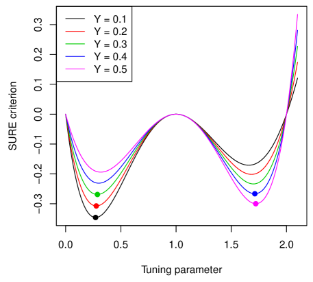
Figure 1: An illustration of a discontinuous mapping $\hat{s}$. Each curve represents the SURE criterion $G(Y,\cdot)$, as a function of the tuning parameter $s$, at nearby values of the (one-dimensional) data realization $Y$. As $Y$ varies, $G(Y,\cdot)$ changes smoothly, but its minimizer $\hat{s}(Y)$ jumps discontinuously, from about $0.75$ at $Y=0.3$ (green curve) to $1.75$ at $Y=0.4$ (blue curve).

With appropriate regularity conditions placed on the family $\{\hat{\theta}_{s}:s\in S\}$, the smoothness of $\hat{s}$ guaranteed in Assumption 1 will imply smoothness of the SURE-tuned estimator $\hat{\theta}_{\hat{s}}$. To state these regularity conditions precisely, we introduce the following notation. Define the “parent” mapping $\widehat{\Theta}:\mathbb{R}^{n}\times S\to\mathbb{R}^{n}$ by $\hat{\theta}_{s}=\widehat{\Theta}(\cdot,s)$ for each $s\in S$. Also define $h:\mathbb{R}^{n}\to\mathbb{R}^{n}\times S$ by $h(Y)=(Y,\hat{s}(Y))$. Note that, in this notation, the SURE-tuned estimator is given by the composition $\hat{\theta}_{\hat{s}}=\widehat{\Theta}\circ h$. The following are our assumptions on $\widehat{\Theta}$.

Assumption 2.

The function $\widehat{\Theta}:\mathbb{R}^{n}\times S\to\mathbb{R}^{n}$ is continuous and weakly differentiable in its first $n$ components—meaning that it is differentiable on (Lebesgue) almost every line segment parallel to one of the first $n$ coordinate axes. In addition, $\mathbb{E}[\sup_{s\in S}\sum_{i=1}^{n}|\partial\widehat{\Theta}_{i}(Y)/\partial Y_{i}|]<\infty$.

The definition of weak differentiability used in Assumption 2 is slightly stronger than the usual definition—which requires absolute continuity (instead of differentiability) on almost every line segment parallel to the coordinate axes. We use the slightly stronger notion for simplicity; together with Assumption 1, it is easy to check that Assumption 2 implies that the map $\hat{\theta}_{\hat{s}}=\widehat{\Theta}\circ h$ is continuous and weakly differentiable, and also $\mathbb{E}[\sum_{i=1}^{n}|\partial\hat{\theta}_{\hat{s},i}(Y)/\partial Y_{i}|]<\infty$.

Therefore we may apply Stein’s formula (10), along with the chain rule, to compute the degrees of freedom of $\hat{\theta}_{\hat{s}}$:

$$\mathrm{df}(\hat{\theta}_{\hat{s}}) =\mathbb{E}\bigg{(}\sum_{i=1}^{n}\frac{\partial(\widehat{\Theta}_{i}\circ h)}{\partial Y_{i}}(Y)\bigg{)}$$

$$=\mathbb{E}\bigg{[}\sum_{i=1}^{n}\bigg{(}\frac{\partial\widehat{\Theta}_{i}}{\partial Y_{i}}(h(Y))+\frac{\partial\widehat{\Theta}_{i}}{\partial s}(h(Y))\frac{\partial\hat{s}}{\partial Y_{i}}(Y)\bigg{)}\bigg{]}$$

$$=\mathbb{E}[\widehat{\mathrm{df}}_{\hat{s}(Y)}(Y)]+\mathbb{E}\bigg{(}\sum_{i=1}^{n}\frac{\partial\widehat{\Theta}_{i}}{\partial Y_{i}}(Y,\hat{s}(Y))\frac{\partial\hat{s}}{\partial Y_{i}}(Y)\bigg{)}.$$

Note that the Stein divergence $\widehat{\mathrm{df}}_{s}(Y)=\sum_{i=1}^{n}\partial\widehat{\Theta}_{i}(Y,s)/\partial Y_{i}$ is an unbiased estimator of $\mathrm{df}(\hat{\theta}_{s})$, for each $s\in S$, under Assumption 2. Hence, comparing the last line above to the definition of excess degrees of freedom in (15), we find that

$$\mathrm{edf}(\hat{\theta}_{\hat{s}})=\mathbb{E}\bigg{(}\sum_{i=1}^{n}\frac{\partial\widehat{\Theta}_{i}}{\partial s}(Y,\hat{s}(Y))\frac{\partial\hat{s}}{\partial Y_{i}}(Y)\bigg{)}.$$ (48)

The above expression provides an explicit characterization of excess degrees of freedom, and in principle, it even gives an unbiased estimator of excess degrees of freedom, i.e., the quantity inside the expectation in (48). Note that the strategy for analyzing the families of shrinkage estimators in Sections 3.1 and 3.3 was precisely the same as that used to arrive at (48) (i.e., simply employing the chain rule), and so it is easy to check that (48) reproduces the results from these sections on excess degrees of freedom.

Unfortunately, the unbiased excess degrees of freedom estimator suggested by (48) is not always tractable. Computing $\partial\widehat{\Theta}_{i}/\partial s$, $i=1,\ldots,n$ in (48) is often easy, at least when the estimator $\hat{\theta}_{s}$ (for fixed $s$) is available in closed-form. But computing $\partial\hat{s}/\partial Y_{i}$, $i=1,\ldots,n$ in (48) is typically much harder; even for simple problems, the SURE-optimal tuning parameter $\hat{s}$ often cannot be written in closed-form. Fortunately, we can use implicit differentiation to rewrite (48) in more useable form. We require the following assumption on the SURE criterion, which recall, we denote by $G$ in (47).

Assumption 3.

The map $G:\mathbb{R}^{n}\times S\to\mathbb{R}$ is continuously differentiable. Furthermore, for each $Y\in\mathbb{R}^{n}$, the minimizer $\hat{s}(Y)$ of $G(Y,\cdot)$ is the unique point satisfying

$$\frac{\partial G}{\partial s}(Y,\hat{s}(Y)) =0,$$ (49)

$$\frac{\partial^{2}G}{\partial s^{2}}(Y,\hat{s}(Y)) >0.$$ (50)

As in our comment following Assumption 1, we must point out that Assumption 3 seems quite strong, and as far as we can tell, in a generic problem setting there seems to be nothing preventing $G(Y,\cdot)$ from being multimodal, which would violate Assumption 3. Still, we will use it to develop insight on the nature of excess degrees of freedom. Differentiating (49) with respect to $Y_{i}$ and using the chain rule gives

$$\frac{\partial^{2}G}{\partial Y_{i}\partial s}(Y,\hat{s}(Y))+\frac{\partial^{2}G}{\partial s^{2}}(Y,\hat{s}(Y))\frac{\partial\hat{s}}{\partial Y_{i}}(Y)=0,$$

and after rearranging,

$$\frac{\partial\hat{s}}{\partial Y_{i}}(Y)=-\bigg{(}\frac{\partial^{2}G}{\partial s^{2}}(Y,\hat{s}(Y))\bigg{)}^{-1}\frac{\partial^{2}G}{\partial Y_{i}\partial s}(Y,\hat{s}(Y)).$$

Plugging this into (48), for each $i=1,\ldots,n$, we have established the following result.

Theorem 3.

Under $Y\sim N(\theta_{0},\sigma^{2}I)$, and Assumptions 1, 2, 3, the excess degrees of freedom of the SURE-tuned estimator $\hat{\theta}_{\hat{s}}$ is given by

$$\mathrm{edf}(\hat{\theta}_{\hat{s}})=-\mathbb{E}\bigg{[}\bigg{(}\frac{\partial^{2}G}{\partial s^{2}}(Y,\hat{s}(Y))\bigg{)}^{-1}\sum_{i=1}^{n}\bigg{(}\frac{\partial\widehat{\Theta}_{i}}{\partial s}(Y,\hat{s}(Y))\frac{\partial^{2}G}{\partial Y_{i}\partial s}(Y,\hat{s}(Y))\bigg{)}\bigg{]}.$$ (51)

A straightforward calculation shows that, for the classes of shrinkage estimators in Sections 3.1 and 3.3, the expression (51) matches the excess degrees of freedom results derived in these sections. In principle, whenever Assumptions 1, 2, 3 hold, Theorem 3 gives an explicitly computable unbiased estimator for excess degrees of freedom, i.e., the quantity inside the expectation in (51). It is unclear to us (as we have already discussed) to what extent these assumptions hold in general, but we can still use (51) to derive some helpful intuition on excess degrees of freedom. Roughly speaking:

• if (on average) $(\partial^{2}G/\partial s^{2})(Y,\hat{s}(Y))$ is large, i.e., $G(Y,\cdot)$ is sharply curved around its minimum, i.e., SURE sharply identifies the optimal tuning parameter value $\hat{s}(Y)$ given $Y$, then this drives the excess degrees of freedom to be smaller;

• if (on average) $|(\partial^{2}G/\partial Y_{i}\partial s)(Y,\hat{s}(Y))|$ is large, i.e., $|(\partial G/\partial s)(Y,\hat{s}(Y))|$ varies quickly with $Y_{i}$, i.e., the function whose root in (49) determines $\hat{s}(Y)$ changes quickly with $Y_{i}$, then this drives the excess degrees of freedom to be larger;

• the pair of terms in the summand in (51) tend to have opposite signs (their specific signs are a reflection of the tuning parametrization associated with $s\in S$), which cancels out the $-1$ in front, and makes the excess degrees of freedom positive.

5.2 Extensions of Stein’s formula, for nonsmooth estimators

When the estimator in question does not satisfy the requisite smoothness conditions, i.e., continuity and weak differentiability, Stein’s formula (10) is not directly applicable. This is especially relevant to the topic of our paper, as the SURE-tuned estimator $\hat{\theta}_{\hat{s}}$ can itself be discontinuous in $Y$ even if each member of the family $\{\hat{\theta}_{s}:s\in S\}$ is continuous in $Y$ (due to discontinuities in the SURE-optimal tuning parameter map $\hat{s}$). This will necessarily be the case for a discrete tuning parameter set $S$, and it can also be the case for a continuous tuning parameter set $S$, recall Figure 1.

Fortunately, extensions of Stein’s formula have been recently developed, to account for discontinuities of certain types. Tibshirani (2015) established an extension for estimators that are piecewise smooth. To define this notion of piecewise smoothness precisely, we must introduce some notation. Given an estimator $\hat{\theta}:\mathbb{R}^{n}\to\mathbb{R}^{n}$, we write $\hat{\theta}_{i}(\,\cdot\,,Y_{-i}):\mathbb{R}\to\mathbb{R}$ for the $i$th component function $\hat{\theta}_{i}$ of $\hat{\theta}$ acting on the $i$th coordinate of the input alone, with all other $n-1$ coordinates fixed at $Y_{-i}$. We also write $\mathcal{D}(\hat{\theta}_{i}(\,\cdot\,,Y_{-i}))$ to denote the set of dicontinuities of the map $\hat{\theta}_{i}(\,\cdot\,,Y_{-i})$. In this notation, the estimator $\hat{\theta}$ is said to be p-almost differentiable if, for each $i=1,\ldots,n$ and (Lebesgue) almost every $Y_{-i}\in\mathbb{R}^{n-1}$, the map $\hat{\theta}_{i}(\,\cdot\,,Y_{-i}):\mathbb{R}\to\mathbb{R}$ is absolutely continuous on each of the open intervals $(-\infty,\delta_{1}),(\delta_{2},\delta_{3}),\ldots,(\delta_{m},\infty)$, where $\delta_{1}<\delta_{2}<\ldots<\delta_{m}$ are the sorted elements of $\mathcal{D}(\hat{\theta}_{i}(\,\cdot\,,Y_{-i}))$, assumed to be a finite set. For p-almost differentiable $\hat{\theta}$, Tibshirani (2015) proved that

$$\mathrm{df}(\hat{\theta})=\mathbb{E}\bigg{[}\sum_{i=1}^{n}\frac{\partial\hat{\theta}_{i}}{\partial Y_{i}}(Y)\bigg{]}+\frac{1}{\sigma}\mathbb{E}\Bigg{[}\sum_{i=1}^{n}\sum_{\delta\in\mathcal{D}(\hat{\theta}_{i}(\,\cdot\,,Y_{-i}))}\phi\bigg{(}\frac{\delta-\theta_{0,i}}{\sigma}\bigg{)}\big{[}\hat{\theta}_{i}(\delta,Y_{-i})_{+}-\hat{\theta}_{i}(\delta,Y_{-i})_{-}\big{]}\Bigg{]},$$ (52)

under some regularity conditions that ensure the second term on the right-hand side is well-defined. Above, we denote one-sided limits from above and from below by $\hat{\theta}_{i}(\delta,Y_{-i})_{+}=\lim_{t\downarrow\delta}\hat{\theta}_{i}(t,Y_{-i})$ and $\hat{\theta}_{i}(\delta,Y_{-i})_{-}=\lim_{t\uparrow\delta}\hat{\theta}_{i}(t,Y_{-i})$, respectively, for the map $\hat{\theta}_{i}(\cdot,Y_{-i})$, $i=1,\ldots,n$, and we denote by $\phi$ the univariate standard normal density.

A difficulty with (52) is that it is often hard to compute or characterize the extra term on the right-hand side. Mikkelsen and Hansen (2016) derived an alternate extension of Stein’s formula for piecewise Lipschitz estimators. While this setting is more restricted than that in Tibshirani (2015), the resulting characterization is more “global” (instead of being based on discontinuities along the coordinate axes), and thus it can be more tractable in some cases. Formally, Mikkelsen and Hansen (2016) consider an estimator $\hat{\theta}:\mathbb{R}^{n}\to\mathbb{R}^{n}$ with associated regular open sets $U_{j}\subseteq\mathbb{R}^{n}$, $j=1,\ldots,J$ whose closures cover $\mathbb{R}^{n}$ (i.e., $\cup_{j=1}^{J}\bar{U}_{j}=\mathbb{R}^{n}$), such that each map $\hat{\theta}^{j}:=\hat{\theta}|_{U_{j}}$ (the restriction of $\hat{\theta}$ to $U_{j}$) is locally Lipschitz continuous. The authors proved that, for such an estimator $\hat{\theta}$,

$$\mathrm{df}(\hat{\theta})=\mathbb{E}\bigg{[}\sum_{i=1}^{n}\frac{\partial\hat{\theta}_{i}}{\partial Y_{i}}(Y)\bigg{]}+\frac{1}{2}\sum_{j\not=k}\int_{\bar{U}_{j}\cap\bar{U}_{k}}\Big{\langle}\hat{\theta}^{k}(y)-\hat{\theta}^{j}(y),\eta_{j}(y)\Big{\rangle}\phi_{\theta_{0},\sigma^{2}I}(y)\,d\mathcal{H}^{n-1}(y),$$ (53)

again under some further regularity conditions that ensure the second term on the right-hand side is well-defined. Above, $\eta_{j}(y)$ denotes the outer unit normal vector to $\partial U_{j}$ (the boundary of $U_{j}$) at a point $y$, $j=1,\ldots,J$, $\phi_{\theta_{0},\sigma^{2}I}$ is the density of a normal variate with mean $\theta_{0}$ and covariance $\sigma^{2}I$, and $\mathcal{H}^{n-1}$ denotes the $(n-1)$-dimensional Hausdorff measure.

Our interest in (52), (53) is in applying these extensions to $\hat{\theta}=\hat{\theta}_{\hat{s}}$, the SURE-tuned estimator defined from a family $\{\hat{\theta}_{s}:s\in S\}$. A general formula for excess degrees of freedom, following from (52) or (53), would be possible, but also complicated in terms of the required regularity conditions. Here is a high-level discussion, to reiterate motivation for (52), (53) and outline their applications. We discuss the discrete and continuous tuning parameter settings separately.

• When the tuning parameter $s$ takes discrete values (i.e., $S$ is a discrete set), extensions such as (52), (53) are needed to characterize excess degrees freedom, because the estimator $\hat{\theta}_{\hat{s}}$ is generically discontinuous and Stein’s original formula cannot be used. In the discrete setting, the first term on the right-hand side of both (52), (53) (when $\hat{\theta}=\hat{\theta}_{\hat{s}}$) is $\mathbb{E}[\widehat{\mathrm{df}}_{\hat{s}(Y)}(Y)]$, in the notation of (15), and thus the second term on the right-hand side of either (52), (53) (when $\hat{\theta}=\hat{\theta}_{\hat{s}}$) gives precisely the excess degrees of freedom.

• When $s$ takes continuous values (i.e., $S$ is a connected subset of Euclidean space), extensions as in (52), (53) are not strictly speaking always needed, though it seems likely to us that they will be needed in many cases, because the SURE-tuned estimator $\hat{\theta}_{\hat{s}}$ can inherit discontinuities from the SURE-optimal parameter map $\hat{s}$ (recall Figure 1). In the continous tuning parameter case, both the first and second terms on the right-hand sides of (52), (53) (when $\hat{\theta}=\hat{\theta}_{\hat{s}}$) can contribute to excess degrees of freedom; i.e., excess degrees of freedom is given by the second term plus any terms left over from applying the chain-rule for differentiation in the first term.

Over the next two subsections, we demonstrate the usefulness of the extensions in (52), (53) by applying them in two specific settings.

5.3 Soft-thresholding estimators

Consider the family of soft-thresholding estimators with component functions

$$\hat{\theta}_{s,i}(Y)=\mathrm{sign}(Y_{i})(|Y_{i}|-s)_{+},\quad i=1,\ldots,n,\quad\text{for}\;s\geq 0.$$ (54)

In this setting, SURE in (6) is

$$\widehat{\mathrm{Err}}_{s}(Y)=\sum_{i=1}^{n}\min\{Y_{i}^{2},s^{2}\}+2\sigma^{2}|\{i:|Y_{i}|\geq s\}|.$$ (55)

Soft-thresholding estimators, like the shrinkage estimators of Section 3.1, have been studied extensively in the statistical literature; some key references that study risk properties of soft-thresholding estimators are Donoho and Johnstone (1994, 1995, 1998), and Chapters 8 and 9 of Johnstone (2015) give a thorough summary.

The extension of Stein’s formula from Tibshirani (2015), as given in (52), can be used to prove that the excess degrees of freedom of the SURE-tuned soft-thresholding estimator is nonnegative. The key realization is as follows: if a component function $\hat{\theta}_{\hat{s},i}$ of the SURE-tuned soft-thresholding estimator jumps discontinuously as we move $Y$ along the $i$th coordinate axes, then the sign of this jump must match the direction in which $Y_{i}$ is moving, thus the latter term on the right-hand side of (52) is always nonnegative. The proof is given in the appendix.

Theorem 4.

The SURE-tuned soft-thresholding estimator $\hat{\theta}_{\hat{s}}$ is p-almost differentiable. Moreover, for each $i=1,\ldots,n$, each $Y_{-i}\in\mathbb{R}^{n-1}$, and each discontinuity point $\delta$ of $\hat{\theta}_{\hat{s}(\cdot,Y_{-i}),i}(\cdot,Y_{-i}):\mathbb{R}\to\mathbb{R}$, it holds that

$$\big{[}\hat{\theta}_{\hat{s}(\delta,Y_{-i}),i}(\delta,Y_{-i})\big{]}_{+}-\big{[}\hat{\theta}_{\hat{s}(\delta,Y_{-i}),i}(\delta,Y_{-i})\big{]}_{-}\geq 0.$$ (56)

Therefore, when $Y\sim N(\theta_{0},\sigma^{2}I)$, we have from (52) that $\mathrm{edf}(\hat{\theta}_{\hat{s}})\geq 0$ and

$$\mathrm{df}(\hat{\theta}_{\hat{s}})\geq\mathbb{E}\big{|}\big{\{}i:|Y_{i}|\geq\hat{s}(Y)\big{\}}\big{|}.$$ (57)

The proof of Theorem 4 provides a precise description of the discontinuities in the SURE-tuned soft-thresholding estimator, which we might be able to use to give a tight upper bound the excess degrees of freedom (second term on the right-hand side in (52)) and upper bound on the risk of the SURE-tuned soft-thresholding estimator, as well. We do not pursue this.

5.4 Subset regression estimators, revisited

We return to the setting of Section 4, i.e., we consider the family of subset regression estimators in (39), which we can abbreviate by $\hat{\theta}_{s}(Y)=P_{s}Y$, $s\in S$, using the notation of the latter section. In Section 4.1, recall, we derived upper bounds on the excess degrees of freedom of the SURE-tuned subset regression estimator $\mathrm{edf}(\hat{\theta}_{\hat{s}})$. Here we apply the extension of Stein’s formula from Mikkelsen and Hansen (2016), as stated in (53), to represent excess degrees of freedom for SURE-tuned subset regression in an alternative and (in principle) exact form. The calculation of the second-term on the right-hand side in (53) for the SURE-tuned subset regression estimator, which yields the result (59) in the next theorem, can already be found in Mikkelsen and Hansen (2016) (in their study of best subset selection). A complete proof is given in the appendix nonetheless.

Theorem 5 (Mikkelsen and Hansen 2016).

The SURE-tuned subset regression estimator $\hat{\theta}_{\hat{s}}$ is piecewise Lipschitz (in fact, piecewise linear) over regular open sets $U_{s}$, $s\in S$, whose closures cover $\mathbb{R}^{n}$. For $s,t\in S$, the outer unit normal vector $\eta_{s}(y)$ to $\partial U_{s}$ at a point $y\in\bar{U}_{s}\cap\bar{U}_{t}$ is given by

$$\eta_{s}(y)=\frac{(P_{t}-P_{s})y}{\|(P_{t}-P_{s})y\|_{2}}.$$ (58)

Therefore, when $Y\sim N(\theta_{0},\sigma^{2}I)$, we have from (53) that

$$\mathrm{edf}(\hat{\theta}_{\hat{s}})=\frac{1}{2}\sum_{s\not=t}\int_{\bar{U}_{s}\cap\bar{U}_{t}}\|(P_{t}-P_{s})y\|_{2}\,\phi_{\theta_{0},\sigma^{2}I}(y)\,d\mathcal{H}^{n-1}(y).$$ (59)

An important implication of the result in (59) is the nonnegativity of excess degrees of freedom in SURE-tuned subset regression, $\mathrm{edf}(\hat{\theta}_{\hat{s}})\geq 0$, which implies that $\mathrm{df}(\hat{\theta}_{\hat{s}})\geq\mathbb{E}(p_{\hat{s}(Y)})$.

While the integral (59) is hard to evaluate in general, it is somewhat more tractable in the case of nested regression models. In the present setting each $s\in S$, recall, is identified with a subset of $\{1,\ldots,p\}$. We say the collection $S$ is nested if for each pair $s,t\in S$, we have either $s\subseteq t$ or $t\subseteq s$. The next result shows that for a nested collection of regression models, the integral expression (59) for excess degrees of freedom simplifies considerably, and can be upper bounded in terms of surface areas of balls under an appropriate Gaussian probability measure.

Before stating the result, it helps to introduce some notation. For a matrix $A$, we write $A_{j:k}$ as shorthand for $A_{\{j,j+1,\ldots,k\}}$, i.e., the submatrix given by extracting columns $j$ through $k$. Likewise, for a vector $a$, we write $a_{j:k}$ as shorthand for $(a_{j},a_{j+1},\ldots,a_{k})$. When $s$ is identified with a nonempty subset $\{1,\ldots,j\}$, we write $P_{s},U_{s},\eta_{s}$ as $P_{j},U_{j},\eta_{j}$ respectively, and use $P_{j}^{\perp}$ for the orthogonal projector to $P_{j}$. Lastly, we refer to the Gaussian surface measure $\Gamma_{d}$, defined over (Borel) sets $A\subseteq\mathbb{R}^{d}$ as

$$\Gamma_{d}(A)=\liminf_{\delta\to 0}\frac{\mathbb{P}(Z\in A_{\delta}\setminus A)}{\delta},$$

where $Z\sim N(0,I)$ denotes a $d$-dimensional standard normal variate, and $A_{\delta}=A+B_{d}(0,\delta)$ is the Minkowski sum of $A$ and the $d$-dimensional ball $B_{d}(0,\delta)$ centered at the origin with radius $\delta$. For a set $A$ with smooth boundary $\partial A$, an equivalent definition is $\Gamma_{d}(A)=\int_{\partial A}\phi_{0,I}(x)\,d\mathcal{H}^{d-1}(x)$, where $\phi_{0,I}$ is the density of $Z$, and $\mathcal{H}^{d-1}$ is the $(d-1)$-dimensional Hausdorff measure. Helpful references on Gaussian surface area include Ball (1993); Nazarov (2003); Klivans et al. (2008). We now state our main result of this subsection, whose proof is given in the appendix.

Theorem 6.

Assume that $Y\sim N(\theta_{0},\sigma^{2}I)$, and that all models in the collection $S$ are nested. Then the excess degrees of freedom of the SURE-tuned subset regression estimator $\hat{\theta}_{\hat{s}}$ is

$$\mathrm{edf}(\hat{\theta}_{\hat{s}})=\sqrt{2}\sigma\sum_{s\subseteq t}\sqrt{p_{t}-p_{s}}\int_{\bar{U}_{s}\cap\bar{U}_{t}}\phi_{\theta_{0},\sigma^{2}I}(y)\,d\mathcal{H}^{n-1}(y).$$ (60)

Now, without a loss of generality (otherwise, the only real adjustment is notational), let us identify each $s$ with a subset $\{1,\ldots,j\}$. Then the excess degrees of freedom is upper bounded by

$$\mathrm{edf}(\hat{\theta}_{\hat{s}})\leq\sum_{d=1}^{p}\sqrt{2d}(d+1)\max_{j=1,\ldots,d}\,\Lambda_{d}\Big{(}B_{d}\big{(}\mu_{(j+1):(j+d)},\sqrt{2d}\big{)}\Big{)},$$ (61)

where $\mu=V^{T}\theta_{0}/\sigma$, and $V\in\mathbb{R}^{n\times p}$ is an orthogonal matrix with columns $v_{j}=P_{j-1}^{\perp}X_{j}/\|P_{j-1}^{\perp}X_{j}\|_{2}$, $j=1,\ldots,p$ (where we let $P_{0}=0$ for notational convenience). Also, recall that $\Lambda_{d}(B_{d}(u,r))$ denotes the $d$-dimensional Gaussian surface area of a ball $B_{d}(u,r)$ centered at $u$ with radius $r$. When $\theta_{0}=0$, the result in (61) can be sharpened and simplified, giving

$$\mathrm{edf}(\hat{\theta}_{\hat{s}})\leq\sum_{d=1}^{p}\sqrt{2d}\bigg{(}1+\frac{1}{d}\bigg{)}\Lambda_{d}\big{(}B_{d}(0,\sqrt{2d})\big{)}<10.$$ (62)

Though it is established in a restricted setting, $\theta_{0}=0$, the result in (62) seems quite strong, as it shows that the excess degrees of freedom of the SURE-tuned subset regression is bounded by the constant $10$, and therefore its excess optimism is bounded by the constant $20\sigma^{2}$, regardless of the number of predictors $p$ in the regression problem.

The derivation of (62) from (61) relies on two key facts: (i) the null case, $\theta_{0}=0$, admits a kind of symmetry that allows us to apply a classic result in combinatorics (the gas stations problem) to compute the exact probability of a collection of chi-squared inequalities, which leads to a reduction in the factor of $d+1$ in each summand of (61) to a factor of $1+1/d$ in each summand of (62); and (ii) the balls in the null case, in the summands of (62), are centered at the origin, so their Gaussian surface areas can be explicitly computed as in Ball (1993); Klivans et al. (2008).

Neither fact is true in the nonnull case, $\theta_{0}\not=0$, making it more difficult to derive a sharp upper bound on excess degrees of freedom. We finish with a couple remarks on the nonnull setting; more serious investigation of explicitly bounding and/or improving (61) is left to future work.

Remark 10 (Nonnull case: two models).

When our collection is composed of just two nested models that are separated by a single variable, i.e., $S=\{\{1,\ldots,p-1\},\{1,\ldots,p\}\}$, straightforward inspection of the proof of Theorem 5 reveals that (61) becomes $\mathrm{edf}(\hat{\theta}_{\hat{s}})=\sqrt{2}\Lambda_{1}(B_{1}(v_{2}^{T}\theta_{0}/\sigma,\sqrt{2}))$ (i.e., note the equality), where $v_{2}=P_{p-1}^{\perp}X_{p}/\|P_{p-1}^{\perp}X_{p}\|_{2}$. The Gaussian surface measure is trivial to compute here (under an arbitrary mean $\theta_{0}$) because it reduces to two evaluations of the Gaussian density, and thus we see that

$$\mathrm{edf}(\hat{\theta}_{\hat{s}})=\sqrt{2}\phi(\sqrt{2}-v_{2}^{T}\theta_{0}/\sigma)+\sqrt{2}\phi(\sqrt{2}+v_{2}^{T}\theta_{0}/\sigma),$$

where $\phi$ is the standard (univariate) normal density. When $\theta_{0}=0$, the excess degrees of freedom is $2\sqrt{2}\phi(\sqrt{2})\approx 0.415$. For general $\theta_{0}$, it is upper bounded by $\max_{u\in\mathbb{R}}\,\sqrt{2}\phi(\sqrt{2}-u)+\sqrt{2}\phi(\sqrt{2}+u)\approx 0.575$.

Remark 11 (Nonnull case: general bounds).

For an arbitrary collection $S$ of nested models and abitrary mean $\theta_{0}$, a very loose upper bound on the right-hand side in (61) is $\sqrt{2p}p(p+1)$, which follows as the Gaussian surface measure of any ball is at most 1, as shown in Klivans et al. (2008). Under restrictions on $\theta_{0}$, tighter bounds on the Gaussian surface measures of the appropriate balls should be possible. Furthermore, the multiplicative factor of $d+1$ in each summand of (61) is also likely larger than it needs to be; we note that an alternate excess degrees of freedom bound to that in (61) (following from similar arguments) is

$$\mathrm{edf}(\hat{\theta}_{\hat{s}})\leq\sqrt{2}\sum_{j<k}\sqrt{k-j}\,\mathbb{P}\big{(}W_{j}(\|\mu_{1:j}\|_{2}^{2})>2(j-1)\big{)}\mathbb{P}\big{(}W_{p-k}(\|\mu_{(k+1):p}\|_{2}^{2})<2(p-k)\big{)}\cdot{}\\ \Lambda_{k-j}\Big{(}B_{k-j}\big{(}\mu_{(j+1):k},\sqrt{2(k-j)}\big{)}\Big{)},$$ (63)

where $W_{d}(\lambda)$ denotes a chi-squared random variable, with $d$ degrees of freedom and noncentrality parameter $\lambda$. Sharp bounds on the noncentral chi-squared tails could deliver a useful upper bound on the right-hand side in (63); we do not expect the final bound reduce to a constant (independent of $p$) as it did in (62) in the null case, but it could certainly improve on the results in Section 4.1, i.e., the bound in (45), which is on the order of $p_{\max}$ (the largest subset size in $S$).

6 Estimating excess degrees of freedom with the bootstrap

We discuss bootstrap methods for estimating excess degrees of freedom. As we have thus far, we assume normality, $Y\sim F=N(\theta_{0},\sigma^{2}I)$ in (1), but in what follows this assumption is used mostly for convenience,and can be relaxed (we can of course replace the normal distribution in the parameteric bootstrap with any known data distribution, or in general, use the residual bootstrap). The main ideas in this section are fairly simple, and follow naturally from standard ideas for estimating optimism using the bootstrap, e.g., Breiman (1992); Ye (1998); Efron (2004).

6.1 Parametric bootstrap procedure

First we descibe a parametric bootstrap procedure. We draw

$$Y^{*,b}\sim N(\hat{\theta}_{\hat{s}(Y)}(Y),\sigma^{2}I),\quad b=1,\ldots,B,$$ (64)

where $B$ is some large number of bootstrap repetitions, e.g., $B=1000$. Our bootstrap estimate for the excess degrees of freedom $\mathrm{edf}(\hat{\theta}_{\hat{s}})$ is then

$$\widehat{\mathrm{edf}}(Y)=\frac{1}{B}\sum_{b=1}^{B}\frac{1}{\sigma^{2}}\sum_{i=1}^{n}\hat{\theta}_{\hat{s}(Y^{*,b}),i}(Y^{*,b})(Y_{i}^{*,b}-\bar{Y}_{i}^{*})-\frac{1}{B}\sum_{b=1}^{B}\widehat{\mathrm{df}}_{\hat{s}(Y^{*,b})}(Y^{*,b}),$$ (65)

where we write $\bar{Y}_{i}^{*}=(1/B)\sum_{b=1}^{B}Y_{i}^{*,b}$ for $i=1,\ldots,n$, and $\widehat{\mathrm{df}}_{s}$ is our estimator for the degrees of freedom of $\hat{\theta}_{s}$, unbiased for each $s\in S$. Note that in (65), for each bootstrap draw $b=1,\ldots B$, we compute the SURE-optimal tuning parameter value $\hat{s}(Y^{*,b})$ for the given bootstrap data $Y^{*,b}$, and we compare the sum of empirical covariances (first term) to the plug-in degrees of freedom estimate (second term). We can express the definition of excess degrees of freedom in (15) as

$$\mathrm{edf}(\hat{\theta}_{\hat{s}})=\mathbb{E}\bigg{(}\frac{1}{\sigma^{2}}\sum_{i=1}^{n}\hat{\theta}_{\hat{s}(Y),i}(Y)(Y_{i}-\theta_{0,i})\bigg{)}-\mathbb{E}[\widehat{\mathrm{df}}_{\hat{s}(Y)}(Y)],$$ (66)

making it clear that (65) estimates (66). Fortuituously, the validity of the bootstrap approximation (65), as noted by Efron (2004), does not depend on the smoothness of $\hat{\theta}_{\hat{s}}$ as a function of $Y$. This makes it appropriate for estimating excess degrees of freedom, even when $\hat{\theta}_{\hat{s}}$ is discontinuous (e.g., due to discontinuities in the SURE-optimal parameter mapping $\hat{s}$), which can be difficult to handle analytically (recall Sections 5.2, 5.3, 5.4).

It should be noted, however, that typical applications of the bootstrap for estimating optimism, as reviewed in Efron (2004), consider low-dimensional problems, and it is not clear that (65) will be appropriate for high-dimensional problems. Indeed, we shall see in the examples in Section 6.3 that the bootstrap estimate for the degrees of freedom $\mathrm{df}(\hat{\theta}_{\hat{s}})$,

$$\widehat{\mathrm{df}}(Y)=\frac{1}{B}\sum_{b=1}^{B}\frac{1}{\sigma^{2}}\sum_{i=1}^{n}\hat{\theta}_{\hat{s}(Y^{*,b}),i}(Y^{*,b})(Y_{i}^{*,b}-\bar{Y}_{i}^{*}),$$ (67)

can be poor in the high-dimensional settings being considered, which is not unexpected. But (perhaps) unexpectedly, in these same settings we will also see that the difference between (67) and the baseline estimate $(1/B)\sum_{b=1}^{B}\widehat{\mathrm{df}}_{\hat{s}(Y^{*,b})}(Y^{*,b})$, i.e., the bootstrap excess degrees of freedom estimate, $\widehat{\mathrm{edf}}(Y)$ in (65), can still be reasonably accurate.

6.2 Alternative bootstrap procedures

Many alternatives to the parametric bootstrap procedure of the last subsection are possible. These alternatives change the sampling distribution in (64), but leave the estimate in (65) the same. We only describe the alternatives briefly here, and refer to the Efron (2004) and references therein for more details.

In the parametric bootstrap, the mean for the sampling distribution in (64) does not have to be $\hat{\theta}_{\hat{s}(Y)}(Y)$; it can be an estimate that comes from a bigger model (i.e., from an estimator with more degrees of freedom), believed to have low bias. The estimate from the “ultimate” bigger model, as Efron (2004) calls it, is $Y$ itself. This gives rise to the alternative bootstrap sampling procedure

$$Y^{*,b}\sim N(Y,c\sigma^{2}I),\quad b=1,\ldots,B,$$ (68)

for some $0<c\leq 1$, as proposed in Breiman (1992); Ye (1998). The choice of sampling distribution in (68) might work well in low dimensions, but we found that it grossly overestimated the degrees of freedom $\mathrm{df}(\hat{\theta}_{\hat{s}})$ in the high-dimensional problem settings considered in Section 6.3, and led to erratic estimates for the excess degrees of freedom $\mathrm{edf}(\hat{\theta}_{\hat{s}})$. For this reason, we preferred the choice in (64), which gave more stable estimates.

Another alternative bootstrap sampling procedure is the residual bootstrap,

$$Y^{*,b}\sim\hat{\theta}_{\hat{s}(Y)}(Y)+\mathrm{Unif}\big{(}\{r_{1}(Y),\ldots,r_{n}(Y)\}\big{)},\quad b=1,\ldots,B,$$ (69)

where we denote by $\mathrm{Unif}(T)$ the uniform distribution over a set $T$, and by $r_{i}(Y)=Y_{i}-\hat{\theta}_{\hat{s}(Y),i}(Y)$, $i=1,\ldots,n$ the residuals. The residual bootstrap (69) is appealing because it moves us away from normality, and does not require knowledge of $\sigma^{2}$. Our assumption throughout this paper is that $\sigma^{2}$ is known—of course, under this assumption, and under a normal data distribution, the parametric sampler (64) outperforms the residual sampler (69), which is we why used the parametric bootstrap in the experiments in Section 6.3. A more realistic take on the problem of estimating optimism and excess optimism would treat $\sigma^{2}$ as unknown, and allow for nonnormal data; for such a setting, the residual bootstrap is an important tool and deserves more careful future study.

6.3 Simulated examples

We empirically evaluate the excess degrees of freedom of the SURE-tuned shrinkage estimator and the SURE-tuned soft-thresholding estimator, across different configurations for the data generating distribution, and evaluate the performance of the parametric bootstrap estimator for excess degrees of freedom. Specifically, our simulation setup can be described as follows.

• We consider 10 sample sizes $n$, log-spaced in between 10 and 5000.

• We consider 3 settings for the mean parameter $\theta_{0}$: the null setting, where we set $\theta_{0}=0$; the weak sparsity setting, where $\theta_{0,i}=4i^{-1/2}$ for $i=1,\ldots,n$; and the strong sparsity setting, where $\theta_{0,i}=4$ for $i=1,\ldots,\lfloor\log{n}\rfloor$ and $\theta_{0,i}=0$ for $i=\lfloor\log{n}\rfloor+1,\ldots,n$.

• For each sample size $n$ and mean $\theta_{0}$, we draw observations $Y$ from the normal data model in (1) with $\sigma^{2}=1$, for a total of 5000 repetitions.

• For each $Y$, we compute the SURE-tuned estimate over the shrinkage family in (21), and the SURE-tuned estimate over the soft-thresholding family in (54).

• For each SURE-tuned estimator $\hat{\theta}_{\hat{s}}$, we record various estimates of degrees of freedom, excess degrees of freedom, and prediction error (details given below).

The simulation results are displayed in Figures 3 and 3; for brevity, we only report on the null and weak sparsity settings for the shrinkage family, and the null and strong sparsity settings for the soft-thresolding family. All degrees of freedom, excess degrees of freedom, and prediction error estimates (except the Monte Carlo estimates) were averaged over the 5000 repetitions; the plots all display the averages along with $\pm 1$ standard error bars.

Figure 3 shows the results for the shrinkage family, with the first row covering the null setting, and the second row the weak sparsity setting. The left column shows the excess degrees of freedom of the SURE-tuned shrinkage estimator, for growing $n$. Four types of estimates of excess degrees of freedom are considered: Monte Carlo, computed from the 5000 repetitions (drawn in black); the unbiased estimate from Stein’s formula, i.e., $2\hat{s}(Y)/(1+\hat{s}(Y))$ (in red); the bootstrap estimate (65) (in green); and the observed (scaled) excess optimism, i.e., $(\|Y^{*}-\hat{\theta}_{\hat{s}(Y)}(Y)\|_{2}^{2}-\widehat{\mathrm{Err}}_{\hat{s}(Y)}(Y))/(2\sigma^{2})$, where $Y^{*}$ is an independent copy of $Y$ (in gray). The middle column shows similar estimates, but for degrees of freedom; here, the naive estimate is $\widehat{\mathrm{df}}_{\hat{s}(Y)}(Y)=n/(1+\hat{s}(Y))$; the unbiased estimate is $n/(1+\hat{s}(Y))+2\hat{s}(Y)/(1+\hat{s}(Y))$; the naive bootstrap estimate is the second term in (65); and the bootstrap estimate is the first term in (65), i.e., as given in (67). Lastly, the right column shows the analogous quantities, but for estimating prediction error. The error metric is normalized by the sample size $n$ for visualization purposes.

We can see that the unbiased estimate of excess degrees of freedom is quite accurate (i.e., close to the Monte Carlo gold standard) throughout. The bootstrap estimate is also accurate in the null setting, but somewhat less accurate in the weak sparsity setting, particularly for large $n$. However, comparing it to the observed (scaled) excess optimism—which relies on test data and thus may not be available in practice—the bootstrap estimate still appears reasonable accurate, and more stable. While all estimates of degrees of freedom are quite accurate in the null setting, we can see that the two bootstrap degrees of freedom estimates are far too small in the weak sparsity setting. This can be attributed to the high-dimensionality of the problem (estimating $n$ means from $n$ observations). Fortuituously, we can see that the difference between the bootstrap and naive bootstrap degrees of freedom estimates, i.e., the bootstrap excess degrees of freedom estimate, is still relatively accurate even when the original two are so highly inaccurate. Lastly, the error plots show that the correction for excess optimism is more significant (i.e., the gap between the naive error estimate and observed test error is larger) in the null setting than in the weak sparsity setting.

Figure 3 shows the results for the soft-thresholding family. The layout of plots is the same as that for the shrinkage family (note that the unbiased estimates of excess degrees of freedom and of degrees of freedom are not available for soft-thresholding). The summary of results is also similar: we can see that the bootstrap excess degrees of freedom estimate is fairly accurate in general, and less accurate in the nonnull case with larger $n$. One noteworthy difference between Figures 3 and 3: for the soft-thresholding family, we can see that the excess degrees of freedom estimates appear to be growing with $n$ (perhaps even linearly), rather than remaining upper bounded by 2, as they are for the shrinkage family (recall also that this is clearly implied by the characterization in (24)).

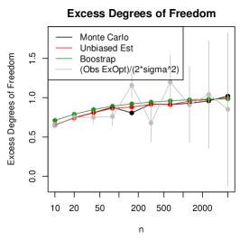
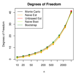
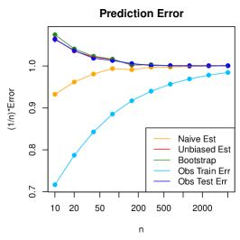
			Null setting
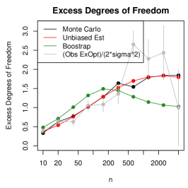
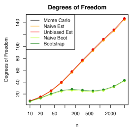
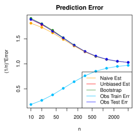
			Weak sparsity setting

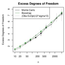
Figure 2: Simulation results for SURE-tuned shrinkage.

			Null setting
			Strong sparsity setting

Figure 3: Simulation results for SURE-tuned soft-thresholding.

7 Discussion

We have proposed and studied a concept called excess optimism, in (14), which captures the added optimism of a SURE-tuned estimator, beyond what is prescribed by SURE itself. By construction, an unbiased estimator of excess optimism leads to an unbiased estimator of the prediction error of the rule tuned by SURE. Further motivation for the study of excess optimism comes from its close connection to oracle estimation, as given in Theorem 1, where we showed that the excess optimism upper bounds the excess risk, i.e., the difference between the risk of the SURE-tuned estimator and the risk of the oracle estimator. Hence, if the excess optimism is shown to be sufficiently small next to the oracle risk, then this establishes the oracle inequality (17) for the SURE-tuned estimator.

Interestingly, excess optimism can be exactly characterized for a family of shrinkage estimators, as studied in Section 3, where we showed that the excess optimism (and hence the excess risk) of a class of shrinkage estimators—in both simple normal means and regression settings—is at most $4\sigma^{2}$. For a family of subset regression estimators, such a precise characterization is not possible, but we showed in Section 4 that upper bounds on the excess optimism can be formed that imply the oracle inequality (17) for the SURE-tuned (here, $C_{p}$-tuned) subset regression estimator.

Characterizating excess optimism—equivalently excess degrees of freedom, in (15), which is just a constant multiple of the former quantity—is a difficult task in general, due to discontinuities that may exist in the SURE-tuned estimator. Such discontinuities disallow the direct the use of Stein’s formula for estimating excess degrees of freedom, and in Section 5 we discussed recently developed extensions of Stein’s formula to handle certain types of discontinuities. As an example application, we proved that one such extension could be used to bound the excess optimism of the SURE-tuned subset regression estimator, over a family of nested subsets, by $20\sigma^{2}$, in the null case when $\theta_{0}=0$. Finally, in Section 6, we showed that estimation of excess degrees of freedom with the bootstrap is conceptually straightforward, and appears to works reasonably well (but, it tends to underestimate excess degrees of freedom in high-dimensional settings with nontrivial signal present in $\theta_{0}$).

We finish by noting an implication of some of our technical results on the degrees of freedom of the best subset selection estimator, and discussing some extensions of our work on excess optimism to two related settings.

7.1 Implications for best subset selection

Our results in Sections 4.1 and 5.4 have implications for the (Lagrangian version of the) best subset selection estimator, namely, given a predictor matrix $X\in\mathbb{R}^{n\times p}$,

$$\hat{\beta}^{\mathrm{subset}}_{\lambda}(Y)=\mathop{\mathrm{argmin}}_{\beta\in\mathbb{R}^{p}}\;\|Y-X\beta\|_{2}^{2}+\lambda\|\beta\|_{0},$$ (70)

where recall, the $\ell_{0}$ norm is defined by $\|\beta\|_{0}=\sum_{j=1}^{p}1\{\beta_{j}\not=0\}$. Here $\lambda\geq 0$ is a tuning parameter. The best subset selection estimator in (70) can be seen as minimizing a SURE-like criterion, cf. the SURE criterion in (40), where we define the collection $S$ to contain all subsets of $\{1,\ldots,p\}$, and we replace the multiplier $2\sigma^{2}$ in (40) with a generic parameter, $\lambda\geq 0$, used to weight the complexity penalty. Combining Lemma 2 (for the upper bound) and Theorem 5 (for the lower bound) provides the following result for best subset selection, whose proof is given in the appendix.

Theorem 7.

Assume that $Y\sim N(\theta_{0},\sigma^{2}I)$. For any fixed value of $\lambda\geq 0$, the degrees of freedom of the best subset selection estimator in (70) satisfies

$$\mathbb{E}\|\hat{\beta}^{\mathrm{subset}}_{\lambda}(Y)\|_{0}\leq\mathrm{df}(X\hat{\beta}^{\mathrm{subset}}_{\lambda})\leq\mathbb{E}\|\hat{\beta}^{\mathrm{subset}}_{\lambda}(Y)\|_{0}+2.29p.$$ (71)

In the language of Tibshirani (2015), the result in (71) proves the search degrees of freedom of best subset selection—the difference between $\mathrm{df}(X\hat{\beta}^{\mathrm{subset}}_{\lambda})$ and $\mathbb{E}\|X\hat{\beta}^{\mathrm{subset}}_{\lambda}(Y)\|_{0}$— is nonnegative, and at most $2.29p$. Nonnegativity of search degrees of freedom here was conjectured by Tibshirani (2015) but not established in full generality (i.e., for general $X$); to be fair, Mikkelsen and Hansen (2016) should be credited with establishing this nonegativity, since, recall, the lower bound in (71) comes from Theorem 5, a result of these authors. The upper bound in (71), as far as we can tell, is new. Though it may seem loose, it implies that the degrees of freedom of the Lagrangian form of best subset selection is at most $3.29p$—in comparison, Janson et al. (2015) prove that best subset selection in constrained form (for a specific configuration of the mean particular $\theta_{0}$) has degrees of freedom approaching $\infty$ as $\sigma\to 0$. This could be a reason to prefer the Lagrangian formulation (70) over its constrained counterpart.

7.2 Heteroskedastic data models

Suppose now that $Y\in\mathbb{R}^{n}$, drawn from a heteroskedastic model

$$Y\sim F,\quad\text{where}\;\mathbb{E}(Y)=\theta_{0},\;\mathrm{Cov}(Y)=\mathrm{diag}(\sigma_{1}^{2},\ldots,\sigma_{n}^{2}).$$ (72)

where $\theta_{0}\in\mathbb{R}^{n}$ is an unknown mean parameter, and $\sigma^{2}_{1},\ldots,\sigma_{n}^{2}>0$ are known variance parameters, now possibly distinct. With the appropriate definitions in place, essentially everything developed so far carries over to this setting.

For an estimator $\hat{\theta}$ of $\theta_{0}$, define its its prediction error, scaled by the variances, by

$$\mathrm{Err}(\hat{\theta})=\mathbb{E}\|\Sigma^{-1}(Y^{*}-\hat{\theta}(Y))\|_{2}^{2}=\mathbb{E}\bigg{[}\sum_{i=1}^{n}\frac{(Y_{i}^{*}-\hat{\theta}_{i}(Y))^{2}}{\sigma_{i}^{2}}\bigg{]},$$ (73)

where $\Sigma=\mathrm{diag}(\sigma_{1}^{2},\ldots,\sigma_{n}^{2})$, and $Y^{*}\sim F$ is independent of $Y$. It is not hard to extend the optimism theorem and SURE, as described in (3), (4), (5), (6), to the current heteroskedastic setting. Similar calculations reveal that the optimism $\mathrm{Opt}(\hat{\theta})=\mathbb{E}\|\Sigma^{-1}(Y^{*}-\hat{\theta}(Y))\|_{2}^{2}-\mathbb{E}\|\Sigma^{-1}(Y-\hat{\theta}(Y))\|_{2}^{2}$ can be expressed as

$$\mathrm{Opt}(\hat{\theta})=2\mathrm{tr}\big{(}\mathrm{Cov}(\hat{\theta}(Y),\Sigma^{-1}Y)\big{)}=2\sum_{i=1}^{n}\frac{\mathrm{Cov}(\hat{\theta}_{i}(Y),Y_{i})}{\sigma_{i}^{2}}.$$ (74)

Given an unbiased estimator $\widehat{\mathrm{Opt}}$ of the optimism $\mathrm{Opt}(\hat{\theta})$, we can define an unbiased estimator $\widehat{\mathrm{Err}}$ of prediction error $\mathrm{Err}(\hat{\theta})$ by

$$\widehat{\mathrm{Err}}(Y)=\|\Sigma^{-1}(Y-\hat{\theta}(Y))\|_{2}^{2}+\widehat{\mathrm{Opt}}(Y),$$ (75)

which we will still refer to as SURE. Assuming that $\hat{\theta}$ is continuous and weakly differentiable, it is implied by Lemma 2 in Stein (1981) that

$$\mathrm{Opt}(\hat{\theta})=2\mathbb{E}\bigg{[}\sum_{i=1}^{n}\frac{\partial\hat{\theta}_{i}(Y)}{\partial Y_{i}}\bigg{]},$$ (76)

i.e., $\widehat{\mathrm{Opt}}(Y)=2\sum_{i=1}^{n}\partial\hat{\theta}_{i}(Y)/\partial Y_{i}$ is an unbiased estimate of optimism.

Sticking with our usual notation $\hat{\theta}_{s},\widehat{\mathrm{Err}}_{s},\widehat{\mathrm{Opt}}_{s}$ to emphasize dependence on a tuning parameter $s\in S$, we can define excess optimism in the current heteroskedastic setting just as before, in (14). An important note is that excess optimism still upper bounds the excess prediction error, i.e., the result in (19) of Theorem 1 still holds.

We briefly sketch an example of an estimator that could be seen as an extension of the simple shrinkage estimator in Section 3.1 to the heteroskedastic setting. In particular, assuming normality in the model in (72), i.e., $Y\sim F=N(\theta_{0},\Sigma)$, with $\Sigma=\mathrm{diag}(\sigma_{1}^{2},\ldots,\sigma_{n}^{2})$, consider

$$\hat{\theta}_{s,i}(Y)=\frac{Y_{i}}{1+\sigma_{i}^{2}s},\quad i=1,\ldots,n,\quad\text{for}\;s\geq 0,$$ (77)

For each $s\geq 0$, note that $\hat{\theta}_{s}$ is the Bayes estimator under the prior $\theta_{0}\sim N(0,s^{-1}I)$. The family in (77) of heteroskedastic (nonuniform) shrinkage estimators is studied in Xie et al. (2012). It is easy to verify that SURE in (75) for this family is

$$\widehat{\mathrm{Err}}_{s}(Y)=\sum_{i=1}^{n}\bigg{(}Y_{i}^{2}\frac{\sigma_{i}^{2}s^{2}}{(1+\sigma_{i}^{2}s)^{2}}+\frac{2}{1+\sigma_{i}^{2}s}\bigg{)}.$$ (78)

(Xie et al. (2012) arrive at a slightly different criterion because they study unscaled prediction error rather than the scaled version we consider in (73).)

Unfortunately, the exact minimizer $\hat{s}(Y)$ of the above criterion cannot be written in closed form, as it could (recall Lemma 1) in Section 3.1. But, assuming that Assumptions 1 and 3 of Section 5.1 hold (we can directly check Assumption 2 for the family of estimators in (77)), implicit differentiation can be used to characterize the excess degrees of freedom of the SURE-tuned heteroskedastic shrinkage estimator $\hat{\theta}_{\hat{s}}$. As before, this leads to

$$\mathrm{ExOpt}(\hat{\theta}_{\hat{s}})=-2\mathbb{E}\bigg{[}\bigg{(}\frac{\partial^{2}G}{\partial s^{2}}(Y,\hat{s}(Y))\bigg{)}^{-1}\sum_{i=1}^{n}\bigg{(}\frac{\partial\widehat{\Theta}_{i}}{\partial s}(Y,\hat{s}(Y))\frac{\partial^{2}G}{\partial Y_{i}\partial s}(Y,\hat{s}(Y))\bigg{)}\bigg{]},$$ (79)

where $\widehat{\Theta}$ denotes the family in (77) as a function of $Y$ and $s$, and $G$ denotes the SURE criterion as a function of $Y$ and $s$. The above generalizes the result in (51) of Theorem 3 for the homoskedastic setting. Computing (79) for the heteroskedastic shrinkage family in (77) gives

$$\mathrm{ExOpt}(\hat{\theta}_{\hat{s}})=\mathbb{E}\left(\frac{\displaystyle\sum_{i=1}^{n}\frac{4Y_{i}^{2}\sigma_{i}^{4}\hat{s}(Y)}{(1+\sigma_{i}^{2}\hat{s}(Y))^{5}}}{\displaystyle\sum_{i=1}^{n}\bigg{[}\frac{\sigma_{i}^{2}}{(1+\sigma_{i}^{2}\hat{s}(Y))^{2}}\bigg{(}Y_{i}^{2}-\frac{4Y_{i}^{2}\sigma_{i}^{2}\hat{s}(Y)}{1+\sigma_{i}^{2}\hat{s}(Y)}+\frac{3Y_{i}^{2}\sigma_{i}^{4}\hat{s}(Y)^{2}}{(1+\sigma_{i}^{2}\hat{s}(Y))^{2}}+\frac{2\sigma_{i}^{2}}{1+\sigma_{i}^{2}\hat{s}(Y)}\bigg{)}\bigg{]}}\right).$$ (80)

We reiterate that the above hinges on Assumptions 1 and 3. It is not clear to us in what generality these assumptions hold for the heteroskedastic shrinkage family (77) (clearly, when $\sigma_{1}^{2}=\ldots=\sigma_{n}^{2}$, these assumptions hold, since in this case the family reduces to the homoskedastic family in (21), and then these assumptions can be easily verified, as discussed previously). Without Assumptions 1 and 3, there would need to be an additional term added to the right-hand side in (80) that accounts for discontinuities in the SURE-tuned heteroskedastic shrinkage estimator $\hat{\theta}_{\hat{s}}$ (e.g., as specified in the second term on the right-hand side in (52)). Deriviation details for (80) are given in the appendix. It can be checked that (80) is indeed equivalent to (24) when all the variances are equal to $\sigma^{2}$.

Interestingly, as we now show, we can view ridge regression through the lens of a heteroskedastic data setup as in (72). Given a predictor matrix $X\in\mathbb{R}^{n\times p}$, it is well-known that the solution to the ridge regression problem (38) is $\hat{\beta}^{\mathrm{ridge}}_{s}(Y)=(X^{T}X+sI)^{-1}X^{T}Y$, for any $s\geq 0$. Denote the singular value decomposition of $X$ by $X=UDV^{T}$. If $Y$ follows the usual homoskedastic distribution in (1) with $F=N(\theta_{0},I)$ (here we have set $\sigma^{2}=1$ for simplicity, and without a loss of generality), then a rotation and diagonal scaling gives

$$W\sim N(\alpha_{0},D^{-2}),$$

where $W=D^{-1}U^{T}Y$, and $\alpha_{0}=D^{-1}U^{T}\theta_{0}$. Further, we can simply deal with (excess) optimism in this new coordinate system, since for any estimator $X\hat{\beta}$ of $\theta_{0}$, we have

$$\mathrm{Opt}(X\hat{\beta})=2\mathrm{tr}\big{(}\mathrm{Cov}(X\hat{\beta}(Y),Y)\big{)}=2\mathrm{tr}\big{(}\mathrm{Cov}(\hat{\alpha}(W),D^{2}W)\big{)}=\mathrm{Opt}(\hat{\alpha}),$$

where $\hat{\alpha}(W)=V^{T}\hat{\beta}(Y)$. Thus, let us define $\hat{\alpha}_{s}(W)=V^{T}\hat{\beta}^{\mathrm{ridge}}_{s}(Y)$, for $s\geq 0$. It is easy to see that $\hat{\alpha}_{s}(W)=(D^{2}+sI)^{-1}D^{2}W$, for $s\geq 0$, i.e.,

$$\hat{\alpha}_{s,i}(W)=\frac{W_{i}}{1+d_{i}^{-2}s},\quad i=1,\ldots,r,\quad\text{for}\;s\geq 0,$$ (81)

where $r$ is the rank of $X$, and $d_{1}\geq\ldots\geq d_{r}>0$ are the diagonal elements of $D$. Hence the setup in (81) is exactly that in (77). The result in (80) shows, under Assumptions 1 and 3 (Assumption 2 can be checked directly), that the excess optimism of the SURE-tuned ridge regression estimator is

$$\mathrm{ExOpt}(X\hat{\beta}^{\mathrm{ridge}}_{\hat{s}})=\\ \mathbb{E}\left(\frac{\displaystyle\sum_{i=1}^{r}\frac{4(u_{i}^{T}Y)^{2}d_{i}^{-6}\hat{s}(Y)}{(1+d_{i}^{-2}\hat{s}(Y))^{5}}}{\displaystyle\sum_{i=1}^{r}\bigg{[}\frac{d_{i}^{-4}}{(1+d_{i}^{-2}\hat{s}(Y))^{2}}\bigg{(}(u_{i}^{T}Y)^{2}-\frac{4(u_{i}^{T}Y)^{2}d_{i}^{-2}\hat{s}(Y)}{1+d_{i}^{-2}\hat{s}(Y)}+\frac{3(u_{i}^{T}Y)^{2}d_{i}^{-4}\hat{s}(Y)^{2}}{(1+d_{i}^{-2}\hat{s}(Y))^{2}}+\frac{2d_{i}^{-2}}{1+d_{i}^{-2}\hat{s}(Y)}\bigg{)}\bigg{]}}\right),$$ (82)

where $u_{1},\ldots,u_{r}\in\mathbb{R}^{n}$ are the columns of $U$. As before, we must stress that it is not at all clear to us in what situations Assumption 1 and 3 will hold for ridge regression, and so (82) should be seen as only one “piece of the puzzle” for ridge regression, as it may be missing important terms (that account for discontinuities in the SURE-tuned ridge estimator). It could still be interesting to work with the right-hand side in (82), and derive bounds on this quantity under various models for the decay of singular values of $X$. This is left to future work, along with a study of the discontinuities of $X\hat{\beta}^{\mathrm{ridge}}_{\hat{s}}$, and the resulting adjustments that need to be made to (82).

7.3 Efron’s $Q$ measures

We stick with the data model in (72). Instead of the normality-inspired squared loss in (73), let us consider a sequence of loss functions $Q_{i}$, $i=1,\ldots,n$, and define the error metric

$$\mathrm{Err}(\hat{\theta})=\mathbb{E}\bigg{[}\sum_{i=1}^{n}Q_{i}(\hat{\theta}_{i}(Y),Y_{i}^{*})\bigg{]},$$ (83)

where $Y^{*}\sim F$, independent of $Y$. We assume that, for each $i=1,\ldots,n$, each $Q_{i}$ is the tangency function of a differentiable, concave function $q_{i}$, i.e.,

$$Q_{i}(u,v)=q_{i}(u)-q_{i}(v)+q_{i}^{\prime}(u)(v-u),$$

where $q_{i}^{\prime}$ denotes the derivative of $q_{i}$. We will refer to $Q_{i}$ as one of Efron’s $Q$ measures, in honor of Efron (1986, 2004), who developed an optimism theorem in the current general setting. (Our setup here is only a very slight generalization of Efron’s, in which we allow for different loss functions $Q_{i}$, for $i=1,\ldots,n$.)

Some examples, as covered in Efron (1986): when $q_{i}(u)=u(1-u)/\sigma_{i}^{2}$, we get the squared loss $Q_{i}(u,v)=(v-u)^{2}/\sigma_{i}^{2}$, and (83) recovers (73); when $q_{i}(u)=\min\{u,1-u\}$, we get the 0-1 loss for $Q_{i}$; when $q_{i}(u)=-2(u\log{u}-(1-u)\log(1-u))$, we get the binomial deviance for $Q_{i}$; in general, for any exponential family distribution, there is a natural concave function $q_{i}$ that can be defined that makes $Q_{i}$ the deviance.

Now let us define

$${\hat{\eta}}_{i}(Y)=-q_{i}^{\prime}(\hat{\theta}_{i}(Y))/2,\quad i=1,\ldots,n.$$

Efron (1986) derived the following beautiful generalization of the optimism theorem (with further discussion in Efron (2004)): the optimism $\mathrm{Opt}(\hat{\theta})=\mathbb{E}[\sum_{i=1}^{n}Q_{i}(\hat{\theta}_{i}(Y),Y^{*}_{i})]-\mathbb{E}[\sum_{i=1}^{n}Q_{i}(\hat{\theta}_{i}(Y),Y_{i})]$ can be alternatively expressed as

$$\mathrm{Opt}(\hat{\theta})=\sum_{i=1}^{n}\mathrm{Cov}({\hat{\eta}}_{i}(Y),Y_{i}).$$ (84)

Hence, given an estimator $\widehat{\mathrm{Opt}}$ of optimism, we can define an estimator $\widehat{\mathrm{Err}}$ of the error $\mathrm{Err}(\hat{\theta})$ by

$$\widehat{\mathrm{Err}}(Y)=\sum_{i=1}^{n}Q_{i}(\hat{\theta}_{i}(Y),Y_{i})+\widehat{\mathrm{Opt}}(Y),$$ (85)

and $\widehat{\mathrm{Err}}$ will be unbiased provided that $\widehat{\mathrm{Opt}}$ is.

Keeping the usual notation $\hat{\theta}_{s},\widehat{\mathrm{Err}}_{s},\widehat{\mathrm{Opt}}_{s}$ to mark the dependence on a tuning parameter $s\in S$, we can define excess optimism for the current setting precisely as before, in (14). Assuming that $\widehat{\mathrm{Opt}}_{s}$ is unbiased, an important realization is that the result in (19) of Theorem 1 holds as written, i.e., the excess optimism still upper bounds the excess prediction error.

In principle, this an exciting extension to pursue. One problem is that it is difficult to form an unbiased estimator of the optimism in (84), and therefore difficult to form an unbiased estimator of prediction error, as defined in (85). By this, we mean specifically that it is difficult to analytically construct an unbiased estimator of optimism (the bootstrap can be used to give an approximately unbiased estimator of optimism, as in Section 6). Under appropriate smoothness conditions on $\hat{\theta}$, Efron (1986) proposed to use the divergence

$$\widehat{\mathrm{Opt}}(Y)=2\sum_{i=1}^{n}\frac{\partial\hat{\theta}_{i}}{\partial Y_{i}}(\hat{\theta}(Y))$$ (86)

to estimate optimism. Note the point of evaluation in (86): it is $\hat{\theta}(Y)$, not $Y$, as in the usual Stein divergence (9). Efron (1986) showed the divergence estimator $\widehat{\mathrm{Opt}}$ defined in (86) is approximately unbiased for $\mathrm{Opt}(\hat{\theta})$, where “approximately” here means its expectation is correct up to first-order in a Taylor expansion. If we could appropriately control the error in this approximation, under say an exponential family distribution for $Y$, then we might be able to extend Theorem 1 the results of Section 4 on subset regression to generalized linear models. We leave this to future work.

Appendix A Proofs

A.1 Proof of Lemma 1

The function $g$ as defined is not convex, but it is smooth, so the result follows from simply checking the image of its critical points, and the boundary points of the contraint region. As for the latter, we note that $g(0)=2b$ and $g(\infty)=a$. As for the former, we compute

$$g^{\prime}(x)=\frac{2ax}{(1+x)^{2}}-\frac{2ax^{2}}{(1+x)^{3}}-\frac{2b}{(1+x)^{2}}.$$

Setting this equal to 0, and solving, yields the single critical point

$$x^{*}=\frac{b}{a-b}.$$

The image of this point is $g(x^{*})=2b-b^{2}/a$, which is always strictly less than $g(0)=2b$ as well as $g(\infty)=a$. Hence $x^{*}$ is the constrained minimizer whenever $x^{*}\geq 0$, i.e., whenever $a\geq b$. If $a<b$, then either 0 or $\infty$ is the minimizer, and as $a<b$ by assumption, the minimizer must be $\infty$.

A.2 Proof of Lemma 2

For each $s\in S$, the moment generating function for $W_{s}$ is

$$\mathbb{E}(e^{tW_{s}})=(1-2t)^{-p_{s}/2}\quad\text{for}\;0\leq t<1/2.$$

Now using Jensen’s inequality,

$$\exp\Big{\{}t\mathbb{E}\Big{[}\max_{s\in S}\,(W_{s}-p_{s})\Big{]}\Big{\}} \leq\mathbb{E}\Big{[}\exp\{t\max_{s\in S}\,(W_{s}-p_{s})\Big{\}}\Big{]}$$

$$=\mathbb{E}\Big{[}\max_{s\in S}\,\exp(t(W_{s}-p_{s}))\Big{]}$$

$$\leq\sum_{s\in S}\mathbb{E}(e^{tW_{s}})e^{-tp_{s}}$$

$$=\sum_{s\in S}((1-2t)e^{-2t})^{-p_{s}/2}.$$

Taking logs of both sides and dividing by $t$, then changing variables to $\delta=1-2t$, gives the result.

A.3 Proof of Theorem 2

Simply define $\delta_{n}=1-a_{n}$, $n=1,2,3,\ldots$. By the first assumption in (46),

$$\frac{1}{1-\delta_{n}}\frac{\log|S|}{\mathrm{Risk}(\hat{\theta}_{s_{0}})}\to 0.$$

Using a Taylor expansion of the function $f(x)=\log(1/x)$ around $x=1$, for $n$ large enough,

$$0\leq\frac{p_{\max}}{\mathrm{Risk}(\hat{\theta}_{s_{0}})}\bigg{(}\frac{\log(1/\delta_{n})}{1-\delta_{n}}-1\bigg{)}\leq\frac{p_{\max}}{\mathrm{Risk}(\hat{\theta}_{s_{0}})}\bigg{(}\frac{1-\delta_{n}}{\delta_{n}}-\frac{1-\delta_{n}}{2\delta_{n}^{2}}\bigg{)}\to 0,$$

where the limit is implied by the second assumption in (46). This proves the result.

A.4 Proof of Theorem 4

The SURE criterion in (55) is piecewise quadratic in $s$, and is monotone for $s$ in between adjacent (absolute) data values $|Y_{i}|$, $i=1,\ldots,n$, and so it must be minimized at one of these data values or at 0 (this is a common observation, e.g., made in Donoho and Johnstone (1995)). Let us denote the order statistics of absolute values by $|Y|_{(1)}\geq\ldots\geq|Y|_{(n)}\geq|Y|_{(n+1)}$, where we set $|Y|_{(n+1)}=0$ for notational convenience. We can reparametrize the family (54) of soft-thresholding estimators so that our tuning parameter now becomes an index $k=1,\ldots,n+1$, where a choice $k$ for the index corresponds to a choice $s=|Y|_{(k)}$ for the threshold level. Accordingly, we can write SURE as

$$\widehat{\mathrm{Err}}_{k}(Y) =k|Y|_{(k)}^{2}+\sum_{j=k+1}^{n}|Y|_{(j)}^{2}+2\sigma^{2}(k-1),$$ (87)

and we seek to minimize this over $k=1,\ldots,n+1$.

Letting $Y_{i}$ vary, and keeping all other coordinates $Y_{-i}$ fixed, we will track discontinuities in the $i$th component of the SURE-tuned soft-thresholding estimator

$$\hat{\theta}_{\hat{k}(\cdot,Y_{-i}),i}(\cdot,Y_{-i}):\mathbb{R}\to\mathbb{R}.$$

Note that these discontinuities can only occur when the minimizer of $\widehat{\mathrm{Err}}_{k}(Y)$ in (87) changes, over $k=1,\ldots,n+1$; also note, a relabeling of the order statistics does not induce such a discontinuity, because all values $\widehat{\mathrm{Err}}_{k}(Y)$, $k=1,\ldots,n+1$ behave continuously as through a relabeling the order statistics due to ties. Therefore, without a loss of generality, we may assume that $Y_{1}\geq\ldots\geq Y_{n}\geq Y_{n+1}=0$ (as we can repeat the same arguments inside each polyhedron over which the labeling of order statistics remains constant). Let us rewrite (87) as

$$\widehat{\mathrm{Err}}_{k}(Y)=kY_{k}^{2}+\sum_{j=k+1}^{n}Y_{j}^{2}+2\sigma^{2}(k-1).$$ (88)

The minimizer $\hat{k}(Y)$ of $\widehat{\mathrm{Err}}_{k}(Y)$, $k=1,\ldots,n+1$ can only jump at an equality between two of these SURE criterion values. As $Y_{i}$ varies, and $Y_{-i}$ remains fixed, such equalities can only happen at a finite number of points. This, along with the absolute continuity of the soft-thresholding operator at a fixed threshold level, establishes p-almost differentiability of $\hat{\theta}_{\hat{k}}$.

Now as $Y_{i}$ varies, let us analyze the rate of change of $\widehat{\mathrm{Err}}_{k}(Y)$, $k=1,\ldots,n+1$, in three cases:

1. if $k>i$, then $\widehat{\mathrm{Err}}_{k}(Y)$ does not change;

2. if $k=i$, then $\widehat{\mathrm{Err}}_{k}(Y)$ changes at a linear rate with slope $2k$;

3. if $k<i$, then $\widehat{\mathrm{Err}}_{k}(Y)$ changes at a linear rate with slope $2$.

We can see that as $Y_{i}$ increases, the minimizer $\hat{k}(Y)$ can only jump from a value $\leq i$ to a value $>i$. This means that the SURE-optimal threshold level can only decrease as $Y_{i}$ increases (recalling the assumed ordering $Y_{1}\geq\ldots\geq Y_{n}\geq 0$), which proves (56). Finally, under normality, $\mathrm{edf}(\hat{\theta}_{\hat{s}})\geq 0$ and (57) follow from (52) with $\hat{\theta}=\hat{\theta}_{\hat{s}}$, and the observation that the SURE-optimal threshold value $\hat{s}(Y)$ is constant in $Y$ at all nondiscontinuity points, so $\partial\hat{s}(Y)/\partial Y_{i}=0$, $i=1,\ldots,n$ almost everywhere.

A.5 Proof of Theorem 5

This proof is essentially already found in Mikkelsen and Hansen (2016) (in their Section 5, where they study the Lagrangian formulation of best subset selection). For completeness, we recapitulate the arguments.

First note that, for any $s,t\in S$, we can express the difference between SURE criterions (40) for models $s$ and $t$, each evaluated at an arbitrary point $y\in\mathbb{R}^{n}$, as

$$\widehat{\mathrm{Err}}_{s}(y)-\widehat{\mathrm{Err}}_{t}(y)=y^{T}(P_{t}-P_{s})y+2\sigma^{2}(p_{s}-p_{t}).$$ (89)

For $s\in S$, let us define $U_{s}$ to be the set of all points $y\in\mathbb{R}^{n}$ such that the SURE criterion evaluated at $y$ is strictly lower for model $s$ than for all other tuning parameter values, i.e.,

$$U_{s}=\bigcap_{t\in S\setminus\{s\}}\Big{\{}y\in\mathbb{R}^{n}:y^{T}(P_{t}-P_{s})y+2\sigma^{2}(p_{s}-p_{t})<0\Big{\}}.$$ (90)

By construction $\hat{\theta}_{\hat{s}}|_{U_{s}}=\hat{\theta}_{s}$, which is a linear function and clearly Lipschitz. It is clear that the sets $U_{s}$, $s\in S$ are regular open (a regular open set is one that is equal to the interior of its closure) and that their closures cover $\mathbb{R}^{n}$. This proves that $\hat{\theta}_{\hat{s}}$ is piecewise Lipschitz.

Now for any $s,t\in S$ and $y\in\bar{U}_{s}\cap\bar{U}_{t}$, we will compute the tangent space to $\partial U_{s}$ at $y$. This can be seen as the collection of derivatives $\gamma^{\prime}(0)$ of smooth curves $\gamma:(-1,1)\to\partial U_{s}$ such that $\gamma(0)=y$. We can compute such derivatives by implicit differentiation. Consider a smooth curve $\gamma$ satisfying $\gamma(0)=y$ and $\gamma(x)\in\partial U_{s}\cap\partial U_{t}$ for $|x|$ sufficiently small. Then for such $x$, $\widehat{\mathrm{Err}}_{s}(\gamma(x))=\widehat{\mathrm{Err}}_{t}(\gamma(x))$, which from (89), can be written as

$$\gamma(x)^{T}(P_{t}-P_{s})\gamma(x)=2\sigma^{2}(p_{t}-p_{s}).$$

Differentiating with respect to $x$, using the chain rule, and evaluating this at $x=0$, gives

$$y^{T}(P_{t}-P_{s})\gamma^{\prime}(0)=0,$$

which defines an $(n-1)$-dimensional subspace in which the derivative $\gamma^{\prime}(0)$ must lie. This shows us that the tangent space to $\partial U_{s}$ at $y$ is $\{z\in\mathbb{R}^{n}:y^{T}(P_{t}-P_{s})z=0\}$, and thus the outer unit normal vector to $\partial U_{s}$ at $y$ is precisely as in (58). (The orientation assigned to $\eta_{s}(y)$ in (58) is important: it is oriented to point from $U_{s}$ to $U_{t}$, which can be verified by examining the directional derivative of $\widehat{\mathrm{Err}}_{s}-\widehat{\mathrm{Err}}_{t}$ in the direction of $\eta_{s}(y)$, evaluated at the point $y$, and checking that this is positive.)

Assuming normality of $Y$, the result in (59) is a direct application of (53). For any $s,t\in S$ and $y\in\bar{U}_{s}\cap\bar{U}_{t}$, it is immediate from (58) that

$$\Big{\langle}\hat{\theta}_{t}(y)-\hat{\theta}_{s}(y),\eta_{s}(y)\Big{\rangle}=\bigg{\langle}(P_{t}-P_{s})y,\frac{(P_{t}-P_{s})y}{\|(P_{t}-P_{s})y\|_{2}}\bigg{\rangle}=\|(P_{t}-P_{s})y\|_{2},$$

which verifies (59).

A.6 Proof of Theorem 6

Assume all models in $S$ are nested. For a pair $s,t\in S$ satisfying (say) $s\subseteq t$, i.e., $\mathrm{col}(X_{s})\subseteq\mathrm{col}(X_{t})$, note that $P_{t}-P_{s}$ is itself a projection matrix (onto $\mathrm{col}(X_{t})\setminus\mathrm{col}(X_{s})$), and so for any $y\in\bar{U}_{s}\cap\bar{U}_{t}$,

$$\|(P_{t}-P_{s})y\|_{2}^{2}=y^{T}(P_{t}-P_{s})y=2\sigma^{2}(p_{t}-p_{s}),$$ (91)

where the first equality comes from idempotence and the second from (90). Plugging this into the result (59) from Theorem 5, for all $s,t\in S$, verifies (60).

We work on bounding the integrals appearing in (60). To rephrase (91), we know that for each $s,t\in S$ with $s\subseteq t$,

$$\bar{U}_{s}\cap\bar{U}_{t}\subseteq\Big{\{}y\in\mathbb{R}^{n}:\|(P_{t}-P_{s})y\|_{2}^{2}=2\sigma^{2}(p_{t}-p_{s})\Big{\}}.$$ (92)

We could certainly integrate the normal density over the set on the right-hand side above in order to bound its integral over $\bar{U}_{s}\cap\bar{U}_{t}$, but it turns out that the simple containment in (92) is a bit too loose. In words, at each point $y\in\bar{U}_{s}\cap\bar{U}_{t}$, we know that the SURE criterions for models $s$ and $t$ must be equal, and this is precisely what is reflected on the right-hand side in (92); however, we are missing the fact that the SURE criterions for all other models $r$ must be no smaller than the common criterion value achieved by models $s,t$.

To develop a more refined approach, we first note that each integral in (60) can be taken over $\bar{U}_{s}\cap\bar{U}_{t}\cap\{y\in\mathbb{R}^{n}:\eta_{s}(y)\not=0\}$ (rather than $\bar{U}_{s}\cap\bar{U}_{t}$), as in each term of (59) the integrand is zero whenever the outer unit normal vector is zero. In our current setup (i.e., disjoint regular open sets whose closures cover $\mathbb{R}^{n}$), it can be shown that the outer unit normal $\eta_{s}$ vanishes on $\bar{U}_{s}\cap\bar{U}_{t}\cap\bar{U}_{r}$, when $s,t,r$ are distinct, except on a set of $\mathcal{H}^{n-1}$ measure zero (e.g., see Lemma A.2 of Mikkelsen and Hansen (2016)). Therefore, we can exactly characterize

$$\bar{U}_{s}\cap\bar{U}_{t}\cap\{y\in\mathbb{R}^{n}:\eta_{j}(y)\not=0\big{\}}=\mathcal{N}\cup\Big{\{}y\in\mathbb{R}^{n}:\|(P_{t}-P_{s})y\|_{2}^{2}=2\sigma^{2}(p_{t}-p_{s}),\\ y^{T}(P_{r}-P_{s})y+2\sigma^{2}(p_{s}-p_{r})<0\;\,\text{and}\;\,y^{T}(P_{r}-P_{t})y+2\sigma^{2}(p_{t}-p_{r})<0,\;\text{for all $r\not=s,t$}\Big{\}},$$ (93)

where $\mathcal{N}$ is a set of $\mathcal{H}^{n-1}$ measure zero. Identifying (say) $s=\{1,\ldots,j\}$ and $t=\{1,\ldots,k\}$, we can rewrite (93) as

$$\bar{U}_{j}\cap\bar{U}_{k}\cap\{y\in\mathbb{R}^{n}:\eta_{j}(y)\not=0\big{\}}={}\\ \mathcal{N}\cup\Big{\{}y\in\mathbb{R}^{n}:\|(P_{k}-P_{j})y\|_{2}^{2}=2\sigma^{2}(k-j),\;\|(P_{j}-P_{\ell})y\|_{2}^{2}>2\sigma^{2}(j-\ell),\;\text{for $\ell<j$},\\ \|(P_{\ell}-P_{j})y\|_{2}^{2}<2\sigma^{2}(\ell-j),\;\text{for $j<\ell<k$},\;\|(P_{\ell}-P_{k})y\|_{2}^{2}<2\sigma^{2}(\ell-k),\;\text{for $\ell>k$}\Big{\}}.$$ (94)

Let $v_{1},\ldots,v_{p}\in\mathbb{R}^{n}$ be orthonormal basis vectors that span $\mathrm{col}(X)$, constructed so that $v_{i}$ spans the column space of $P_{i}-P_{i-1}$ for each $i=1,\ldots,p$ (where we take $P_{0}=0$ for notational convenience), i.e., $v_{i}=P_{i-1}^{\perp}X_{i}/\|P_{i-1}^{\perp}X_{i}\|_{2}$, $i=1,\ldots,p$ as in the theorem statement. Then (94) becomes

$$\bar{U}_{j}\cap\bar{U}_{k}\cap\{y\in\mathbb{R}^{n}:\eta_{j}(y)\not=0\big{\}}={}\\ \mathcal{N}\cup\bigg{\{}y\in\mathbb{R}^{n}:\sum_{i=j+1}^{k}(v_{i}^{T}y)^{2}=2\sigma^{2}(k-j),\;\sum_{i=\ell+1}^{j}(v_{i}^{T}y)^{2}>2\sigma^{2}(j-\ell),\;\text{for $\ell<j$},\\ \sum_{i=j+1}^{\ell}(v_{i}^{T}y)^{2}<2\sigma^{2}(\ell-j),\;\text{for $j<\ell<k$},\;\sum_{i=k+1}^{\ell}(v_{i}^{T}y)^{2}<2\sigma^{2}(\ell-k),\;\text{for $\ell>k$}\bigg{\}}.$$

Integrating the normal density over the set on the right-hand side above, with respect to the appropriate ($(n-1)$-dimensional Hausdorff) measure, gives

$$\sigma\int_{\bar{U}_{j}\cap\bar{U}_{k}\cap\{\eta_{j}(y)\not=0\}}\phi_{\theta_{0},\sigma^{2}I}(y)\,d\mathcal{H}^{n-1}(y)={}\\ \sigma\int_{\begin{subarray}{c}\sum_{i=\ell+1}^{j}(v_{i}^{T}y)^{2}>2\sigma^{2}(j-\ell),\;\ell<j\\ \sum_{i=j+1}^{k}(v_{i}^{T}y)^{2}=2\sigma^{2}(k-j),\;\sum_{i=j+1}^{\ell}(v_{i}^{T}y)^{2}<2\sigma^{2}(\ell-j),\;j<\ell<k,\\ \sum_{i=k+1}^{\ell}(v_{i}^{T}y)^{2}<2\sigma^{2}(\ell-j),\;\ell>k\end{subarray}}\phi_{\theta_{0},\sigma^{2}I}(y)\,d\mathcal{H}^{n-1}(y).$$ (95)

We note that a sufficient condition for SURE at $y$ to be minimized at one of $j,\ldots,k$, i.e., for $y$ to be an element of $\cup_{\ell=j}^{k}\bar{U}_{\ell}$, is

$$\sum_{i=\ell+1}^{j}(v_{i}^{T}y)^{2}>2\sigma^{2}(j-\ell),\;\text{for $\ell<j$},\;\sum_{i=k+1}^{\ell}(v_{i}^{T}y)^{2}<2\sigma^{2}(\ell-k),\;\text{for $\ell>k$},$$

and so carrying on from (95),

$$\sigma\int_{\bar{U}_{j}\cap\bar{U}_{k}\cap\{\eta_{j}(y)\not=0\}}\phi_{\theta_{0},\sigma^{2}I}(y)\,d\mathcal{H}^{n-1}(y)$$

$$\leq\sigma\mathbb{P}\Big{(}Y\in\cup_{\ell=j}^{k}\bar{U}_{\ell}\Big{)}\int_{\sum_{i=j+1}^{k}(v_{i}^{T}y)^{2}=2\sigma^{2}(k-j),\;\sum_{i=j+1}^{\ell}(v_{i}^{T}y)^{2}<2\sigma^{2}(\ell-j),\;j<\ell<k}\phi_{\theta_{0},\sigma^{2}I}(y)\,d\mathcal{H}^{n-1}(y)$$

$$=\sigma\mathbb{P}\Big{(}Y\in\cup_{\ell=j}^{k}\bar{U}_{\ell}\Big{)}\int_{\sum_{i=j+1}^{k}z_{i}^{2}=2\sigma^{2}(k-j),\;\sum_{i=j+1}^{\ell}z_{i}^{2}<2\sigma^{2}(\ell-j),\;j<\ell<k}\phi_{M^{T}\theta_{0},\sigma^{2}I}(z)\,d\mathcal{H}^{n-1}(z),$$

where $M\in\mathbb{R}^{n\times n}$ in defined to be an orthogonal matrix whose first $p$ are given by $v_{1},\ldots,v_{p}$, i.e., given by the matrix $V\in\mathbb{R}^{n\times p}$ introduced in the theorem. As the sets $\bar{U}_{\ell}$, $\ell=1,\ldots,d$ intersect on a set of ($n$-dimensional Lebesgue) measure zero, we can rewrite the above as

$$\sigma\int_{\bar{U}_{j}\cap\bar{U}_{k}\cap\{\eta_{j}(y)\not=0\}}\phi_{\theta_{0},\sigma^{2}I}(y)\,d\mathcal{H}^{n-1}(y)\leq{}\\ \sigma\sum_{\ell=j}^{k}\mathbb{P}(Y\in U_{\ell})\int_{\sum_{i=j+1}^{k}z_{i}^{2}=2\sigma^{2}(k-j),\;\sum_{i=j+1}^{\ell}z_{i}^{2}<2\sigma^{2}(\ell-j),\;j<\ell<k}\phi_{M^{T}\theta_{0},\sigma^{2}I}(z)\,d\mathcal{H}^{n-1}(z).$$ (96)

In general, the integral in (96) is difficult to compute (though we will have luck in the case that $\theta_{0}=0$, to be discussed shortly), so we can simply upper bound it by discarding the inequalities in the domain of integration, giving

$$\sigma\int_{\bar{U}_{j}\cap\bar{U}_{k}\cap\{\eta_{j}(y)\not=0\}}\phi_{\theta_{0},\sigma^{2}I}(y)\,d\mathcal{H}^{n-1}(y) \leq\sigma\sum_{\ell=j}^{k}\mathbb{P}(Y\in U_{\ell})\int_{\sum_{i=j+1}^{k}z_{i}^{2}=2\sigma^{2}(k-j)}\phi_{M^{T}\theta_{0},\sigma^{2}I}(z)\,d\mathcal{H}^{n-1}(z)$$

$$=\sum_{\ell=j}^{k}\mathbb{P}(Y\in U_{\ell})\;\Lambda_{k-j}\Big{(}B_{k-j}\big{(}\mu_{(j+1):k},\sqrt{2(k-j)}\big{)}\Big{)},$$

where the last line used the definition of Gaussian surface area, recalling the notation $\mu=V^{T}\theta_{0}/\sigma$ as in the theorem. Summing the above bound over all pairs $j<k$ with separation $k-j=d$ gives

$$\sigma\sum_{j=1}^{p-d}\int_{\bar{U}_{j}\cap\bar{U}_{j+d}\cap\{\eta_{j}(y)\not=0\}}\phi_{\theta_{0},\sigma^{2}I}(y)\,d\mathcal{H}^{n-1}(y) \leq\sum_{j=1}^{p-d}\sum_{\ell=j}^{j+d}\mathbb{P}(Y\in U_{\ell})\;\Lambda_{d}\Big{(}B_{d}\big{(}\mu_{(j+1):(j+d)},\sqrt{2d}\big{)}\Big{)}$$

$$\leq(d+1)\max_{j=1,\ldots,d}\,\Lambda_{d}\Big{(}B_{d}\big{(}\mu_{(j+1):(j+d)},\sqrt{2d}\big{)}\Big{)},$$

where in the last line, we recognized that each index $\ell$ appears in the double sum $d+1$ times. An upper bound on the full sum (over all pairs $j,k$) in (60) is given by multiplying the last line above by $\sqrt{2d}$, and summing this over $d=1,\ldots,p$, which establishes (61).

When the balls in (61) are all centered at the origin, i.e., when $\theta_{0}=0$ (or more generally, this would happen in a nested family $S$ such that $P_{s}\theta_{0}=\theta_{0}$ for all $s\in S$), we can upper bound (61) by invoking known results on the Gaussian surface area of balls. Importantly, though, it turns out to be more fruitful to return to an earlier step along the way to deriving (61), namely, the integral on the right-hand side in (96), which recall we upper bounded in the general $\theta_{0}$ case by dropping the inequality constraints in the domain of integration. Let us write this integral as

$$\mathbb{P}\Bigg{(}\sum_{i=j+1}^{\ell}W_{i}<2(\ell-j),\;\text{for $j<\ell<k$}\;\Bigg{|}\;\sum_{i=j+1}^{k}W_{i}=(k-j)\Bigg{)}\Lambda_{k-j}\Big{(}B_{k-j}\big{(}0,\sqrt{2(k-j)}\big{)}\Big{)},$$ (97)

where $W_{i}$, $i=j+1,\ldots,k$ are i.i.d. $\chi^{2}_{1}$ random variates. To simplify notation, we denote $k-j=d$ and relabel these random variates as $W_{1},\ldots,W_{d}$. Because $W_{1},\ldots,W_{d}$ are i.i.d., they are still i.i.d. conditional on their sum being equal to $2d$, and when we further condition on $(W_{1},\ldots,W_{d})$ being equal to $(w_{1},\ldots,w_{d})$ up to a circular permutation, any ones of the $d$ options

$$(w_{1},w_{2},\ldots,w_{d}),\;(w_{d},w_{1},\ldots,w_{d-1}),\;\ldots,\;(w_{2},w_{3},\ldots,w_{1})$$

is equally likely. Now we recall and apply the following classic result in combinatorics.

Proposition 1 (The gas stations problem).

Let $w_{1},\ldots,w_{d}$ be nonnegative numbers that sum to $2d$. Then there exists exactly one circular permutation of $(w_{1},\ldots,w_{d})$, call it $(w_{i_{1}},\ldots,w_{i_{d}})$, such that

$$w_{i_{1}}+\ldots+w_{i_{q}}\leq 2q,\;\text{for all $q=1,\ldots,d$}.$$

By Proposition 1 and the discussion preceding it, we see that (97) becomes simply

$$\frac{1}{d}\Lambda_{d}\big{(}B_{d}(0,\sqrt{2d})\big{)},$$ (98)

and by following the exact same steps leads up to (61), we obtain the sharper upper bound that is given by the first inequality of (62).

For the Gaussian surface area of an origin-centered ball, Ball (1993) gave the formula

$$\Lambda_{d}\big{(}B_{d}(0,r)\big{)}=\frac{r^{d-1}e^{-r^{2}/2}}{2^{d/2-1}\Gamma(d/2)},$$

in any dimension $d$ (see Klivans et al. (2008) for a simple, direct proof). Plugging this formula into the first inequality in (62) gives

$$\sum_{d=1}^{p}\sqrt{2d}\bigg{(}1+\frac{1}{d}\bigg{)}\Lambda_{d}\big{(}B_{d}(0,\sqrt{2d})\big{)}\leq 2\sum_{d=1}^{p}\bigg{(}1+\frac{1}{d}\bigg{)}\frac{d^{d/2}e^{-d}}{\Gamma(d/2)}.$$

Continuing on with the chain of upper bounds, we apply the following Stirling-type bound for the gamma function (e.g., Jameson (2015)),

$$\frac{x^{x-1/2}e^{-x}}{\Gamma(x)}\leq\frac{1}{\sqrt{2\pi}}\quad\text{for all $x>0$},$$

which yields

$$2\sum_{d=1}^{p}\bigg{(}1+\frac{1}{d}\bigg{)}\frac{d^{d/2}e^{-d}}{\Gamma(d/2)}\leq\frac{1}{\sqrt{\pi}}\sum_{d=1}^{p}\bigg{(}\sqrt{d}+\frac{1}{\sqrt{d}}\bigg{)}\bigg{(}\frac{2}{e}\bigg{)}^{d/2}.$$ (99)

We split the right-hand side above into two sums and bound each individually. Consider first

$$\frac{1}{\sqrt{\pi}}\sum_{d=1}^{p}\sqrt{d}\bigg{(}\frac{2}{e}\bigg{)}^{d/2}\leq\frac{1}{\sqrt{\pi}}\sum_{d=1}^{\infty}\sqrt{d}\bigg{(}\frac{2}{e}\bigg{)}^{d/2}\leq\frac{1}{\sqrt{\pi}}\sum_{d=1}^{N}\sqrt{d}\bigg{(}\frac{2}{e}\bigg{)}^{d/2}+\frac{1}{\sqrt{\pi}}\sum_{d=N+1}^{\infty}d\bigg{(}\frac{2}{e}\bigg{)}^{d/2}.$$ (100)

The second term on the right-hand side above can be calculated as

$$\frac{1}{\sqrt{\pi}}\sum_{d=N+1}^{\infty}d\bigg{(}\frac{2}{e}\bigg{)}^{d/2} =\sqrt{\frac{2}{\pi e}}\sum_{d=N+1}^{\infty}d\bigg{(}\sqrt{\frac{2}{e}}\bigg{)}^{d-1}$$

$$=\sqrt{\frac{2}{\pi e}}\frac{d}{dx}\bigg{(}\sum_{d=N+1}^{\infty}x^{d}\bigg{)}\bigg{|}_{x=\sqrt{2/e}}$$

$$=\frac{1}{\sqrt{\pi}}\frac{\sqrt{2/e}^{N+1}}{1-\sqrt{2/e}}\bigg{(}N+1-\frac{\sqrt{2/e}}{1-\sqrt{2/e}}\bigg{)}.$$ (101)

Thus we can upper bound the right-hand side in (100) by computing the first sum with $N=1000$ numerically and computing the second via (101), which gives

$$\frac{1}{\sqrt{\pi}}\sum_{d=1}^{1000}\sqrt{d}\bigg{(}\frac{2}{e}\bigg{)}^{d/2}+\frac{1}{\sqrt{\pi}}\sum_{d=1001}^{\infty}d\bigg{(}\frac{2}{e}\bigg{)}^{d/2}<8.21.$$ (102)

It remains to consider

$$\frac{1}{\sqrt{\pi}}\sum_{d=1}^{p}\frac{1}{\sqrt{d}}\bigg{(}\frac{2}{e}\bigg{)}^{d/2}\leq\frac{1}{\sqrt{\pi}}\sum_{d=1}^{\infty}\frac{1}{\sqrt{d}}\bigg{(}\frac{2}{e}\bigg{)}^{d/2}\leq\frac{1}{\sqrt{\pi}}\sum_{d=1}^{N}\frac{1}{\sqrt{d}}\bigg{(}\frac{2}{e}\bigg{)}^{d/2}+\frac{1}{\sqrt{\pi}}\sum_{d=N+1}^{\infty}\bigg{(}\frac{2}{e}\bigg{)}^{d/2}.$$ (103)

As before, the second term in (103) we can compute as $(1/\sqrt{\pi})\sqrt{2/e}^{N+1}(1-\sqrt{2/e})^{-1}$, and the first term we can evaluate numerically at $N=1000$, which gives

$$\frac{1}{\sqrt{\pi}}\sum_{d=1}^{1000}\frac{1}{\sqrt{d}}\bigg{(}\frac{2}{e}\bigg{)}^{d/2}+\frac{1}{\sqrt{\pi}}\sum_{d=1001}^{\infty}\bigg{(}\frac{2}{e}\bigg{)}^{d/2}<1.75.$$ (104)

Putting (102) and (104) together, we can upper bound the right-hand side in (99) by $8.21+1.75=9.96<10$, which establishes the second inequality in (62), and completes the proof.

A.7 Proof of Theorem 7

For the lower bound, we note that an argument analogous to that given in the proof of Theorem 5 shows that the excess degrees of freedom of subset selection, i.e., the quantity

$$\mathrm{df}(X\hat{\beta}^{\mathrm{subset}}_{\lambda})-\mathbb{E}\|X\hat{\beta}^{\mathrm{subset}}_{\lambda}(Y)\|_{0},$$

is exactly equal to the right-hand side in (59), where the sum is taken over all pairs of subsets. See Section 5 of Mikkelsen and Hansen (2016). Nonnegativity of the integrand in each term of the sum therefore proves the lower bound in (71).

Meanwhile, the search degrees of freedom is upper bounded by the quantity considered in (43) of Lemma 2, where $S$ is the set of all subsets of $\{1,\ldots,p\}$. The upper bound is thus

$$\min_{\delta\in[0,1)}\;\frac{2}{1-\delta}\log\sum_{s\in S}(\delta e^{1-\delta})^{-p_{s}/2} =\min_{\delta\in[0,1)}\;\frac{2}{1-\delta}\log\sum_{k=0}^{p}{p\choose k}\Big{(}(\delta e^{1-\delta})^{-1/2}\Big{)}^{k}$$

$$=\min_{\delta\in[0,1)}\;\frac{2p}{1-\delta}\log\Big{(}1+(\delta e^{1-\delta})^{-1/2}\Big{)},$$

where the last step used the binomial theorem. Sraightforward numerical calculation shows that

$$\min_{\delta\in[0,1)}\;\frac{2}{1-\delta}\log\Big{(}1+(\delta e^{1-\delta})^{-1/2}\Big{)}<1.145,$$

completing the proof.

A.8 Derivation details for (80)

First, we compute

$$\frac{\partial\widehat{\Theta}_{i}}{\partial s}(Y,s))=-\frac{Y_{i}\sigma_{i}^{2}}{(1+\sigma_{i}^{2}s)^{2}}.$$

Next,

$$\frac{\partial G}{\partial s}(Y,s)=\sum_{i=1}^{n}\bigg{(}\frac{2Y_{i}^{2}\sigma_{i}^{2}s}{(1+\sigma_{i}^{2}s)^{2}}-\frac{2Y_{i}^{2}\sigma_{i}^{4}s^{2}}{(1+\sigma_{i}^{2}s)^{3}}-\frac{2\sigma_{i}^{2}}{(1+\sigma_{i}^{2}s)^{2}}\bigg{)}.$$

Then,

$$\frac{\partial^{2}G}{\partial Y_{i}\partial s}(Y,s)=\frac{4Y_{i}\sigma_{i}^{2}s}{(1+\sigma_{i}^{2}s)^{2}}\bigg{(}1-\frac{\sigma_{i}^{2}s}{1+\sigma_{i}^{2}s}\bigg{)}=\frac{4Y_{i}\sigma_{i}^{2}s}{(1+\sigma_{i}^{2}s)^{3}}.$$

Finally,

$$\frac{\partial^{2}G}{\partial s^{2}}(Y,s) =\sum_{i=1}^{n}\bigg{(}\frac{2Y_{i}^{2}\sigma_{i}^{2}}{(1+\sigma_{i}^{2}s)^{2}}-\frac{4Y_{i}^{2}\sigma_{i}^{4}s}{(1+\sigma_{i}^{2}s)^{3}}-\frac{4Y_{i}^{2}\sigma_{i}^{4}s}{(1+\sigma_{i}^{2}s)^{3}}+\frac{6Y_{i}^{2}\sigma_{i}^{6}s^{2}}{(1+\sigma_{i}^{2}s)^{4}}+\frac{4\sigma_{i}^{4}}{(1+\sigma_{i}^{2}s)^{3}}\bigg{)}$$

$$=\sum_{i=1}^{n}\bigg{[}\frac{2\sigma_{i}^{2}}{(1+\sigma_{i}^{2}s)^{2}}\bigg{(}Y_{i}^{2}-\frac{4Y_{i}^{2}\sigma_{i}^{2}s}{1+\sigma_{i}^{2}s}+\frac{3Y_{i}^{2}\sigma_{i}^{4}s^{2}}{(1+\sigma_{i}^{2}s)^{2}}+\frac{2\sigma_{i}^{2}}{1+\sigma_{i}^{2}s}\bigg{)}\bigg{]}.$$

Therefore, plugging the relevant quantities into (79), we get (80).

References

- Ball (1993) Keith Ball. The reverse isoperimetric problem for Gaussian measure. Discrete & Computational Geometry, 10(4):411–420, 1993.
- Baranchik (1964) Alvin Baranchik. Multiple regression and estimation of the mean of a multivariate normal distribution. Technical Report, Stanford University, 1964.
- Berk et al. (2013) Richard Berk, Lawrence Brown, Andreas Buja, Kai Zhang, and Linda Zhao. Valid post-selection inference. Annals of Statistics, 41(2):802–837, 2013.
- Bernau et al. (2013) Christoph Bernau, Thomas Augustin, and Anne-Laure Boulesteix. Correcting the optimal resampling-based error rate by estimating the error rate of wrapper algorithms. Biometrics, 69(3):693–702, 2013.
- Birge (2001) Lucien Birge. An alternative point of view on Lepski’s method. IMS Lecture Notes–Monograph Series, 36:113–133, 2001.
- Breiman (1992) Leo Breiman. The little bootstrap and other methods for dimensionality selection in regression: -fixed prediction error. Journal of the American Statistical Society, 87(419):738–754, 1992.
- Candes et al. (2013) Emmanuel J. Candes, Carlos M. Sing-Long, and Joshua D. Trzasko. Unbiased risk estimates for singular value thresholding and spectral estimators. IEEE Transactions on Signal Processing, 61(19):4643–4657, 2013.
- Cavalier et al. (2002) Laurent Cavalier, Yuri Golubev, Dominique Picard, and Alexandre Tsybakov. Oracle inequalities for inverse problems. Annals of Statistics, 30(3):843–874, 2002.
- Chen et al. (2015) Xi Chen, Qihang Lin, and Bodhisattva Sen. On degrees of freedom of projection estimators with applications to multivariate shape restricted regression. arXiv: 1509.01877, 2015.
- Donoho and Johnstone (1994) David L. Donoho and Iain M. Johnstone. Ideal spatial adaptation by wavelet shrinkage. Biometrika, 81(3):425–455, 1994.
- Donoho and Johnstone (1995) David L. Donoho and Iain M. Johnstone. Adapting to unknown smoothness via wavelet shrinkage. Journal of the American Statistical Association, 90(432):1200–1224, 1995.
- Donoho and Johnstone (1998) David L. Donoho and Iain M. Johnstone. Minimax estimation via wavelet shrinkage. Annals of Statistics, 26(8):879–921, 1998.
- Efron (1986) Bradley Efron. How biased is the apparent error rate of a prediction rule? Journal of the American Statistical Association, 81(394):461–470, 1986.
- Efron (2004) Bradley Efron. The estimation of prediction error: Covariance penalties and cross-validation. Journal of the American Statistical Association, 99(467):619–632, 2004.
- Efron (2010) Bradley Efron. Large-scale Simultaneous Inference: Empirical Bayes Methods for Estimation, Testing, and Prediction. Cambridge University Press, 2010.
- Efron (2014) Bradley Efron. Estimation and accuracy after model selection. Journal of the American Statistical Association, 109(507):991–1007, 2014.
- Efron and Hastie (2016) Bradley Efron and Trevor Hastie. Computer Age Statistical Inference: Algorithms, Inference, and Data Science. Cambridge University Press, 2016.
- Fithian et al. (2014) William Fithian, Dennis Sun, and Jonathan Taylor. Optimal inference after model selection. arXv: 1410.2597, 2014.
- Harris (2016) Xiaoying Tian Harris. Prediction error after model selection. arXv: 1610.06107, 2016.
- Hoerl and Kennard (1970) Arthur Hoerl and Robert Kennard. Ridge regression: biased estimation for nonorthogonal problems. Technometrics, 12(1):55–67, 1970.
- James and Stein (1961) W. James and Charles Stein. Estimation with quadratic loss. Proceedings of the Fourth Berkeley Symposium on Mathematical Statistics and Probability, 1:361–379, 1961.
- Jameson (2015) Graham Jameson. A simple proof of Stirling’s formula for the gamma function. The Mathematical Gazette, 99(544):68–74, 2015.
- Janson et al. (2015) Lucas Janson, William Fithian, and Trevor Hastie. Effective degrees of freedom: A flawed metaphor. Biometrika, 102(2):479–485, 2015.
- Johnstone (1999) Iain M. Johnstone. Wavelet shrinkage for correlated data and inverse problems: Adaptivity results. Statistica Sinica, 9:51–83, 1999.
- Johnstone (2015) Iain M. Johnstone. Gaussian Estimation: Sequence and Wavelet Models. Cambridge University Press, 2015. Draft version.
- Klivans et al. (2008) Adam Klivans, Ryan O’Donnell, and Rocco Servedio. Learning geometric concepts via Gaussian surface area. Foundations of Computer Science, 49:541–550, 2008.
- Kneip (1994) Alois Kneip. Ordered linear smoothers. Annals of Statistics, 22(5):835–866, 1994.
- Krstajic et al. (2014) Damjan Krstajic, Ljubomir Buturovic, David Leahy, and Simon Thomas. Cross-validation pitfalls when selecting and assessing regression and classification models. Journal of Cheminformatics, 6(10), 2014.
- Laurent and Massart (2000) Beatrice Laurent and Pascal Massart. Adaptive estimation of a quadratic functional by model selection. Annals of Statistics, 28(5):1302–1338, 2000.
- Lee et al. (2016) Jason Lee, Dennis Sun, Yukai Sun, and Jonathan Taylor. Exact post-selection inference, with application to the lasso. Annals of Statistics, 44(3):907–927, 2016.
- Li (1985) Ker-Chau Li. From Stein’s unbiased risk estimates to the method of generalized cross-validation. Annals of Statistics, 14(4):1352–1377, 1985.
- Li (1986) Ker-Chau Li. Asymptotic optimality of and generalized cross-validation in ridge regression with application to spline smoothing. Annals of Statistics, 14(3):1101–1112, 1986.
- Li (1987) Ker-Chau Li. Asymptotic optimality for , , cross-validation and generalized cross-validation: discrete index set. Annals of Statistics, 15(3):958–975, 1987.
- Lockhart et al. (2014) Richard Lockhart, Jonathan Taylor, Ryan J. Tibshirani, and Robert Tibshirani. A significance test for the lasso. Annals of Statistics, 42(2):413–468, 2014.
- Mallows (1973) Colin Mallows. Some comments on . Technometrics, 15(4):661–675, 1973.
- Mikkelsen and Hansen (2016) Frederik Riis Mikkelsen and Niels Richard Hansen. Degrees of freedom for piecewise Lipschitz estimators. arXiv: 1601.03524, 2016.
- Nazarov (2003) Fedor Nazarov. On the maximal perimeter of a convex set in with respect to Gaussian measure. Geometric Aspects of Functional Analysis, 1806:169–187, 2003.
- Shao and Strawderman (1994) Peter Yi-Shi Shao and William Strawderman. Improving on the James-Stein positive-part estimator. Annals of Statistics, 22(3):1517–1538, 1994.
- Stein (1981) Charles Stein. Estimation of the mean of a multivariate normal distribution. Annals of Statistics, 9(6):1135–1151, 1981.
- Tibshirani (2015) Ryan J. Tibshirani. Degrees of freedom and model search. Statistica Sinica, 25(3):1265–1296, 2015.
- Tibshirani and Taylor (2011) Ryan J. Tibshirani and Jonathan Taylor. The solution path of the generalized lasso. Annals of Statistics, 39(3):1335–1371, 2011.
- Tibshirani and Taylor (2012) Ryan J. Tibshirani and Jonathan Taylor. Degrees of freedom in lasso problems. Annals of Statistics, 40(2):1198–1232, 2012.
- Tibshirani and Tibshirani (2009) Ryan J. Tibshirani and Robert Tibshirani. A bias correction for the minimum error rate in cross-validation. Annals of Applied Statistics, 3(2):822–829, 2009.
- Tibshirani et al. (2016) Ryan J. Tibshirani, Jonathan Taylor, Richard Lockhart, , and Robert Tibshirani. Exact post-selection inference for sequential regression procedures. Journal of the American Statistical Association, 111(514):600–620, 2016.
- Tsamardinos et al. (2015) Ioannis Tsamardinos, Amin Rakhshani, and Vincenzo Lagani. Performance-estimation properties of cross-validation-based protocols with simultaneous hyper-parameter optimization. International Journal on Artificial Intelligence Tools, 24(5), 2015.
- Ulfarsson and Solo (2013a) Magnus O. Ulfarsson and Victor Solo. Tuning parameter selection for nonnegative matrix factorization. IEEE International Conference on Acoustics, Speech and Signal Processing, 2013a.
- Ulfarsson and Solo (2013b) Magnus O. Ulfarsson and Victor Solo. Tuning parameter selection for underdetermined reduced-rank regression. IEEE Signal Processing Letters, 20(9):881–884, 2013b.
- Varma and Simon (2006) Sudhir Varma and Richard Simon. Bias in error estimation when using cross-validation for model selection. BMC Bioinformatics, 7(91), 2006.
- Xie et al. (2012) Xianchao Xie, Samuel Kou, and Lawrence Brown. SURE estimates for a heteroscedastic hierarchical model. Journal of the American Statistical Association, 107(500):1465–1479, 2012.
- Ye (1998) Jianming Ye. On measuring and correcting the effects of data mining and model selection. Journal of the American Statistical Society, 93(441):120–131, 1998.
- Zou and Yuan (2008) Hui Zou and Ming Yuan. Regularized simultaneous model selection in multiple quantiles regression. Computational Statistics and Data Analysis, 52(12):5296–5304, 2008.
- Zou et al. (2007) Hui Zou, Trevor Hastie, and Robert Tibshirani. On the “degrees of freedom” of the lasso. Annals of Statistics, 35(5):2173–2192, 2007.