Thermal Winds in Stellar Mass Black Hole and Neutron Star Binary Systems

Abstract

Black hole binaries show equatorial disc winds at high luminosities, which apparently disappear during the spectral transition to the low/hard state. This is also where the radio jet appears, motivating speculation that both wind and jet are driven by different configurations of the same magnetic field. However, these systems must also have thermal winds, as the outer disc is clearly irradiated. We develop a predictive model of the absorption features from thermal winds, based on pioneering work of Begelman et al 1983. We couple this to a realistic model of the irradiating spectrum as a function of luminosity to predict the entire wind evolution during outbursts. We show that the column density of the thermal wind scales roughly with luminosity, and does not shut off at the spectral transition, though its visibility will be affected by the abrupt change in ionising spectrum. We re-analyse the data from H1743-322 which most constrains the difference in wind across the spectral transition and show that these are consistent with the thermal wind models. We include simple corrections for radiation pressure, which allows stronger winds to be launched from smaller radii. These winds become optically thick around Eddington, which may even explain the exceptional wind seen in one observation of GRO J1655-40. These data can instead be fit by magnetic wind models, but similar winds are not seen in this or other systems at similar luminosities. Hence we conclude that the majority (perhaps all) current data can be explained by thermal or thermal-radiative winds.

1 Introduction

Absorption lines from ionised material are seen in many high inclination Low Mass X-ray Binary systems, both neutron stars (NS) and black holes (BHB). These are most evident in the deep absorption dips which occur at specific orbital phases due to clumps formed where the accretion stream hits the disc. However, some absorption lines remain even outside of the dip events. These are seen mainly as hydrogen and helium-like iron K$\alpha$, indicating very highly ionised material which is distributed fairly uniformly around all azimuths. These lines can be blue shifted by up to a few thousand km/s, showing clearly that there is an equatorial disc wind in these systems, where the material is strongly photo-ionised by the X-ray illumination from the central source (see e.g. the reviews by Diaz Trigo & Boirin 2013; 2016 and Ponti et al 2012).

The most important questions about these winds concerns how they are launched, and their connection to the accretion flow and its jet. Both black hole and neutron star binaries show a dramatic spectral transition, from a disc dominated spectrum at high luminosity to a much harder Comptonised spectrum at lower luminosities. This can be explained as the transition between a disc and hot accretion flow (see e.g. the review by Done, Gierlinski & Kubota 2007). Data from GRS1915+105 was first used to study the change in wind properties with spectral state, with Neilson & Lee (2009) showing that the wind disappeared as the source made a transition to the harder spectral state. They noted that this spectral transition also marks the onset of the compact radio jet, so speculated on the existence of a causal link, with the change in accretion flow properties also changing the magnetic field configuration so that the same magnetically driven outflow is either a wind in the soft, disc dominated state or a jet in the low/hard state. Miller et al (2012) similarly find that the wind is not present in a hard state of H1743-322, while it is clearly evident in a soft state from the same source. The systematic survey of existing data by Ponti et al (2012) showed that none of the sources with winds in the high/soft state had significant absorption features in the low/hard state, though there are not many sources, and the most constraining data are from GRS1915+105 and H1743-322 discussed above.

An alternative explanation for the lack of wind features in the low/hard state is that the changing spectral shape at the transition changes the ionisation of the wind (e.g. Diaz Trigo et al. 2014). However, other photoionisation calculations show that the difference in wind properties between hard and soft spectral state cannot be completely explained by the same wind being present at different ionisation level (Chakravorty et al 2013; Higginbottom & Proga 2015). This motivated studies of magnetic winds (Chakravorty et al 2016), though it is now clear that both winds and jets can co-exist at high luminosities (Kalemci et al 2016, Homan et al 2016).

However, winds in binary systems need not be magnetically driven. X-ray irradiation of the outer disk can produce a thermally driven wind/corona. The X-ray flux from the innermost regions illuminates the upper layers of the outer disk, heating it up to the Compton temperature, $T_{\rm IC}$, which depends only on spectral shape. The heated upper layer expands on the sound speed $c_{IC}=(kT_{IC}/\mu)^{1/2}$ where $\mu$ is the mean particle mass (ions and electrons), fixed at $0.61m_{p}$ for solar abundances. The material is then unbound at radii where this sound speed is larger than the escape speed i.e. $R>R_{IC}=GM/c_{IC}^{2}$. This gives $R_{IC}=6.4\times 10^{4}/T_{IC,8}R_{g}$ (where $R_{g}=GM/c^{2}$ and $T_{IC,8}=T_{IC}/10^{8}~{}{\rm K}$) so the material escapes as a wind (Begelman et al. 1983, hereafter B83). A more careful treatment shows that the wind can be launched from $R>0.2R_{IC}$ as long as the luminosity is high enough to sustain rapid heating (B83, Woods et al 1996, hereafter W96). Conversely, at smaller radii/lower luminosity the majority of the material remains bound but forms an extended atmosphere above the disk (B83, W96; Jimenez-Garate et al 2002).

Current data from the high inclination NS systems show a good qualitative match to the thermal wind predictions, with small disc systems (short period binaries) having absorbing material which is static, while outflows are only seen at radii larger than $0.2R_{IC}$ (Diaz Trigo & Boirin 2013; 2016). Many winds in the black hole systems also have a fairly large launch radius, consistent with thermal driving (e.g. Kubota et al 2007; Diaz Trigo & Boirin 2016), and the most powerful winds are seen in the systems with the biggest discs (Diaz Trigo & Boirin 2016). This is consistent with the predictions of thermal winds (see below), but not a natural consequence of magnetic wind models.

However, there is a single observation of dramatic absorption from GRO J1655-40 at low luminosities. The material has high column, and lower ionisation state than is normally seen, so has multiple lines from lower atomic number elements as well as the standard H- and He-like iron absorption. These require that the wind is launched from $<<0.1R_{IC}$ if the observed luminosity is a good estimate of the intrinsic luminosity, so this cannot be a thermal wind (Miller et al 2006; Kallman et al 2009; Luketic et al 2010; Neilsen & Homan 2012; Higginbottom & Proga 2015). However, the unusual properties of the broadband continuum seen during this observation indicate that the intrinsic source luminosity may be substantially underestimated (Done, Gierlinski & Kubota 2007; Shidatsu et al 2016; Neilsen et al 2016). If the intrinsic source luminosity is actually close to Eddington then strong winds can be launched from much smaller radii than predicted by the thermal wind models. Electron scattering in a completely ionised, optically thick inner wind could suppress the observed luminosity to below Eddington, with the observed absorption lines tracing only lower ionisation material in the outer photosphere. Whatever the origin of the wind in this single observation, it does not represent the majority of winds seen in binaries, nor is it seen in observations at similar luminosity of the same source (Nielsen & Homan 2012). Yet this single dataset, coupled with the observed anti-correlation between wind and jet discussed above, has led to a focus on magnetic winds in the current literature.

Even if there are magnetic winds, thermal winds should also be present (e.g. Neilsen & Homan 2012), as we know that the outer disc is illuminated - the observed optical emission is dominated by reprocessed X-ray flux (van Paradijs & McClintock 1994). In marked contrast with magnetic winds, thermal winds are rather well understood theoretically in terms of overall mass loss rates. However, models for thermal winds were developed long before the advent of detectors which could observe them, and they have been mostly sidelined due to the focus on magnetic winds, with only a few recent papers on their properties (Luketic et al 2010; Higginbottom & Proga 2015).

Here, we combine analytic and numerical thermal wind models to make quantitative predictions for the mass loss rates for thermal winds, and their most basic observables (i.e. column density and ionisation state). We couple this to a simple model of how the spectrum changes with luminosity during outbursts to quantitatively explore the effect of the spectral transition. The thermal wind models roughly predict that the column density of the wind is proportional to the mass accretion rate. Thus the amount of material in the wind should not change much as the source switches from high/soft to low/hard at roughly constant luminosity during the spectral tranistion, though its visibility will be affected by the change in photo-ionising spectrum (Chakravorty et al 2013; Diaz Trigo et al 2014; Higginbottom & Proga 2015). We compare this to the current observational constraints from H1743-322 on the wind in a high/soft state being supressed in a low/hard state (Miller et al 2012). We find that the thermal wind models are consistent with their data as this high/soft state is probably an order of magnitude higher mass accretion rate than the comparison low/hard state, so should have an order of magnitude stronger wind. A more stringent test would be to follow the wind evolution during a single transition, rather than to compare the wind seen in low/hard and high/soft spectra at different mass accretion rates separated by years.

We incorporate a simple correction for radiation pressure as the source approaches the Eddington limit. This allows the wind to be launched from smaller radii than $R<0.2R_{IC}$ as it reduces the effective gravity. We show that these thermal-radiative winds do indeed become optically thick as $L\to L_{Edd}$, so they could potentially explain the anomolous wind in GROJ1655-40. GRS1915+105 is similarly close to Eddington, but its more complex and fast variable spectra require a specialised analysis which is beyond the scope of this paper (e.g. Ueda et al 2010; Zoghbi et al 2016). These are the three main systems claimed to rule out the thermal wind models and hence require magnetic driving. We conclude that this is premature, and that thermal (and thermal-radiative) wind models already explain the vast majority (and perhaps all) of winds currently seen in binary systems.

2 Thermal wind models

B83 discuss the different physical regimes in which Compton heated, thermal winds can form. We repeat here their analysis for completeness, pulling out only the required terms from their much longer, more detailed analysis.

The central source spectrum contains photons over a broad range of energies, and illuminates the disc at distance $R$ with differential photon number rate $N(\nu)$ corresponding to energy flux $F(\nu)=h\nu N(\nu)=L(\nu)/(4\pi R^{2})$ in ergs cm² s^-1 Hz^-1 or $L(E)/(4\pi R^{2})$ in ergs cm² s^-1 erg^-1. Electrons in the disc photosphere at this radius have initial temperature $T_{e}$. Photons with energies $E=h\nu\gg T_{e}$ will Compton downscattered, losing some energy to the disc, typically $\Delta E/E=-E/(m_{e}c^{2})$. Conversely, those at low energies will be Compton upscattered by the hot electrons in the disc, with typical $\Delta E/E=4kT_{e}/(m_{e}c^{2})$, so they cool the photosphere. Combing these gives an approximation for the energy change from both processes as $\Delta E=4kT_{e}E/(m_{e}c^{2})-E^{2}/(m_{e}c^{2})$. This reaches steady state when heating balances cooling, so $\int\Delta EN(E)dE=0$, defining the Compton temperature $kT_{IC}=\frac{1}{4}\int EL(E)dE/L$ where $L=\int L(E)dE$ (see e.g. Done 2010).

Compton cooling is the dominant cooling process only at high temperatures, where the material is completely ionised. Deeper down in the photosphere the heating from irradiation will be lower as the upper layers have already absorbed some of the energy, so the gas temperature, $T_{e}$, goes down. The disc is in hydrostatic equilibrium so the gas pressure, $P_{gas}=nkT_{e}$, must be higher to support the weight of the upper layers. Thus the density, $n$, must increase downwards by more than the decrease in temperature from the lower irradiation. Higher density means that Bremsstrahlung cooling becomes important, which lowers the temperature still further, requiring an even larger increase in density to give the required pressure support for the weight of the upper layers. Eventually the temperature is so low that electrons can start to be bound to ions, making line cooling possible. This triggers an ionisation instability, as the line cooling lowers the temperature, but this allows more electrons to be bound, making more line transitions and hence more cooling (Krolik, McKee & Tarter 1981). Thus the disc photosphere splits into a hot, high ionisation skin overlying a cool, dense photosphere (Nayakshin, Kazanas & Kallman 2000). The typical temperature of the skin is the Compton temperature $kT_{IC}$, and its typical pressure can be calculated from the pressure ionisation parameter $\Xi=P_{rad}/P_{gas}=L/(4\pi R^{2}cP_{gas})$. The instability is triggered at $\Xi\sim 40$, giving the gas density $n=L/(160\pi R^{2}ckT_{IC})$ (B83; W96).

The mass loss per unit area, $\dot{m}$ is then driven by the material in the skin expanding on the thermal sound speed. For an isothermal flow, the pressure at the sonic point is a factor of 2 lower than at the base, so this gives $\dot{m}=\frac{1}{2}n\mu c_{IC}$. The total mass loss rate in the wind is then

$$\begin{split}\dot{M}_{wind}=\int_{R_{in}}^{R_{out}}\dot{m}\times 2\times 2\pi RdR\\ \approx\frac{L/c}{80\ c_{IC}}\log R_{out}/R_{in}\end{split}$$ (1)

where the factor of $2$ comes from the fact that the disc has two sides. From the discussion above, $R_{in}\sim 0.2R_{IC}$ and $R_{out}$ is the disc outer radius, and the total mass loss rate in the wind is directly proportional to the source luminosity.

However, the wind is only isothermal if it is heated sufficiently quickly. This depends on the irradiating flux, which drops with increasing radius, so the wind is not heated so efficiently. The Compton heating rate on each electron, $\Gamma_{e}$, is the incident photon flux, $\sigma_{T}L/(\langle E\rangle 4\pi R^{2})$, where $\langle E\rangle$ is the mean photon energy, times the mean increase in energy for each photon collision $\approx 4kT_{IC}\langle E\rangle/(m_{e}c^{2})$ from the Compton heating discussion above. Hence $\Gamma_{e}=\sigma_{T}LkT_{IC}/(\pi R^{2}m_{e}c^{2})$. For large luminosities, the material is heated impulsively and reaches the Compton temperature at the isothermal sonic point which is close to the disc, as assumed above. For lower luminosities, electrons in the gas are heated steadily, reaching a characteristic energy $kT_{ch}=\Gamma_{e}R/c_{ch}$ where $R/c_{ch}$ is the time taken for the material to reach height $\sim R$. This equation determines the characteristic temperature, $T_{ch}$ and its corresponding sound speed $c_{ch}=(kT_{ch}/\mu)^{1/2}$, but the gas pressure above the ionisation instability is still set by the radiation flux as before so $P_{ch}=nkT_{ch}=L/(160\pi R^{2}c)$. This gives

$$kT_{ch}=kT_{IC}(L/L_{crit})^{2/3}\zeta^{-2/3}$$ (2)

where $L_{crit}$ is the luminosity which is just able to heat the gas to $kT_{IC}$ as it reaches height $\sim R$ so that it is able to escape, at distance $\zeta=R/R_{IC}=1$. Equivalently, this gives

$$c_{ch}=c_{IC}(L/L_{crit})^{1/3}\zeta^{-1/3}$$ (3)

Figure 1: The different wind regions of B83, with boundaries shown as the thick black lines. For $L>L_{crit}$ the wind is impulsively heated to $T_{IC}$ at $R/R_{IC}<L/L_{crit}$ (e.g. upper green solid line). The mean particle velocity is smaller than the escape speed for small radii ($R/R_{IC}<1$) so the heated skin forms an isothermal atmosphere (region E) with only small wind losses, whereas it escapes as an isothermal wind for $1<R/R_{IC}<L/L_{crit}$ (region A). For $R/R_{IC}>L/L_{crit}$ the wind is steadily heated, only reaching temperature $T_{ch}(R)$, but this can still escape as a wind (region B) for $L/L_{crit}>1$. Instead, for $L/L_{crit}<1$ (e.g. the lower green line), the illumination only heats the disc to $T_{ch}$ rather than $T_{IC}$, so there is even less wind escape from the inner region with $R/R_{IC}<1$ (region D). The material still cannot escape at $R=R_{IC}$ as $T_{ch}<T_{IC}$ (region C, gravity inhibited wind), and only becomes unbound for $R/R_{IC}\geq(L/L_{crit})^{-1}$ (region B again), though this inner boundary depends somewhat on the Compton temperature, with the dashed (solid) thick black line being appropriate for low (high) Compton temperatures (W96). The red vertical line shows that at small radii, $R_{out}=0.1R_{IC}$, the disc will go from region E and D as the luminosity increases, whereas the blue line shows that at large radii, $R_{out}=10R_{IC}$, the disc material goes from being inhibited by gravity (region C), to being steadily heated (region B), to impulsively heated (region A) as the luminosity increases.

Figure 2: a) The mass loss rate from a $10^{8}M_{\odot}$ black hole per unit area of disc at scaled radius $\zeta=R/R_{IC}$ for $\log L/L_{Edd}=-3$ (black) $-2$ (red), $-1$ (green), $0$ (blue) and $1$ (cyan) as in W96. These correspond to $L/L_{crit}=0.0125-125$ for the assumed constant $T_{IC,8}=0.13$. b) The corresponding cumulative mass loss rate from the disc at $R<R_{out}=5R_{IC}$.

Figure 3: The effect of disc size on the efficiency of wind production per unit mass accretion rate. The range of irradiating luminosity is the same as in Fig. 1 i.e. $L/L_{Edd}=10^{-3}\to 10$, which corresponds to $L/L_{crit}=1.25\times 10^{-2}\to 1.25\times 10^{2}$ for the assumed $T_{IC,8}=0.13$. The disc size is $R_{out}=0.1R_{IC}$ (black), $0.3R_{IC}$ (red), $R_{IC}$ (green), $3R_{IC}$ (blue) and $10R_{IC}$ (cyan). All disc sizes show that the disc is increasingly efficient at producing a wind with increasing mass accretion rate for $L/L_{crit}\to 1$, but then the efficiency stabilises to a constant for $L/L_{crit}\gg 1$. This constant value is larger than the mass input rate for all disc sizes where $R_{out}\geq R_{IC}$, so the wind losses should have a major impact on the observed luminosity. B83 suggest that the mass loss rates from the smallest disc sizes, with $R_{out}\ll R_{IC}$, are underestimated. The dashed black line shows the impact of their suggested correction factor for small discs ($R_{out}=0.1R_{IC}$) where there is no confining pressure from an outer wind.

The critical luminosity can be written in terms of the Eddington limit $L_{Edd}=4\pi GMm_{I}c/\sigma_{T}$, where $m_{I}\approx 2\mu$ is the mean ion mass per electron, giving

$$\begin{split}L_{crit}=\frac{1}{8}(m_{e}/\mu)^{1/2}(m_{e}c^{2}/kT_{IC})^{1/2}L_{Edd}\\ \sim 0.03T_{IC,8}^{-1/2}L_{Edd}\end{split}$$ (4)

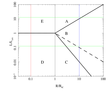
Thus the entire outer disc out to $R_{out}$ remains impulsively heated only for $L>L_{out}=(R_{out}/R_{IC})L_{crit}$ (region A in B83, see Fig. 1). For $L_{crit}<L<L_{out}$ this wind is only impulsively heated from $R_{in}\sim R_{IC}$ to to a radius $(L/L_{crit})R_{IC}$. For larger radii the heating is not fast enough to heat it to $kT_{IC}$, so it only reaches $kT_{ch}$, but gravity is lower at these larger radii, so it still escapes as a wind as $kT_{ch}\geq GM\mu/R$ (upper Region B in B83). The upper horizontal thin (green) line on Fig. 1 shows an example for $L/L_{crit}=12.5$, where the wind is impulsively heated for $1<R/R_{IC}<12.5$ and then steadily heated for radii $R/R_{IC}>12.5$.

Similarly, for $L<L_{crit}$ the wind is only heated to a temperature of $T_{ch}<T_{IC}$ at $R_{IC}$, so cannot escape (Region C in B83, the gravity inhibited wind). This escape condition $kT_{ch}>GM\mu/R$, defines an effective inner launch radius for the wind of $R_{in}/R_{IC}\sim(L/L_{crit})^{-2}$. This is appropriate at high Compton temperatures, $T_{IC,8}\sim 1$, where only Compton processes are important as assumed in B83, but at lower Compton temperatures then atomic cooling become important, giving $R_{in}/R_{IC}\sim(L/L_{crit})^{-1}$ (W96, Higginbottom & Proga 2015). Either way, this is again the steady heating region (Region B). The lower horizontal thin (green) line on Fig. 1 shows an example for $L/L_{crit}=0.125$, where the wind is launched only for radii $R/R_{IC}>12.5$ (low Compton temperature), or $>2.82$ (high Compton temperature).

The instability is still triggered at $\Xi\sim 40$, giving the density as $n_{ch}\propto L/(R^{2}T_{ch}$), so the specific mass loss rate in region B is $\dot{m}=n_{ch}\mu c_{ch}$ (no factor of $1/2$ this time, see B83), giving a total mass loss rate in the wind of

$$\begin{split}\dot{M}_{wind}=\int_{R_{in}}^{R_{out}}n_{ch}\mu c_{ch}\times 2\times 2\pi RdR\\ =3\frac{L^{2/3}L^{1/3}_{crit}/c}{40c_{IC}}\Bigl{[}\Bigl{(}\frac{R_{out}}{R_{IC}}\Bigr{)}^{1/3}-\Bigl{(}\frac{R_{in}}{R_{IC}}\Bigr{)}^{1/3}\Bigr{]}\end{split}$$ (5)

Thus the wind mass loss rate in region B scales only with $L^{2/3}$ rather than with $L$ as in region A.

For $R\ll R_{IC}$ and $L>L_{crit}$ the upper layers of the disc are heated to $T_{IC}$ but this is less than the escape velocity at this point. Thus the material forms an isothermal, exponential atmosphere above the disc with only a very small fraction of the material being able to escape (region E). At lower luminosities ($L<L_{crit}$) this atmophere is steadily heated to characteristic temperature $T_{ch}<T_{IC}$, so there is even less wind (region D). Fig. 1 shows these regions schematically (B83, W96).

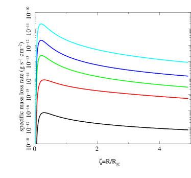
Regions A and B (impulsive Compton heating and steady Compton heating) are the two main regimes which contribute to the thermal wind, though other radii/luminosities ranges can power smaller mass loss rates. W96 give fitting formula for the specific mass loss rate in all regimes of luminosity and Compton temperature of the radiation in their equation 4.8. These were derived from smoothly matching to results from full hydrodynamical simulations of thermal winds. We integrate these over all radii, rather than using the different equations 1 and 5 with upper and lower radial limits. We show the results for the specific mass loss rate per unit area, $\dot{m}$ as a function of radius in Fig.2a, reproducing the results in Fig 6 of W96 for a $10^{8}$M_⊙ black hole with $\log L/L_{Edd}=-3,-2,-1,0,1$, which is equivalent to $L/L_{crit}=1.25\times 10^{-2}-1.25\times 10^{2}$ for the assumed $T_{IC,8}=0.13$. Obviously, radiation pressure should also enhance the wind as the luminosity approaches and exceeds $L_{Edd}$, which was not considered in W96 or B83. We return to this point in Section 4. There is a clear peak in the specific mass loss rate at $R\sim 0.2R_{IC}$.

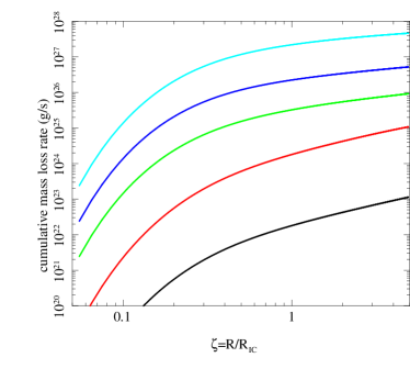
Fig.2b shows the corresponding cumulative mass loss in the wind, $\dot{M}$ as a function of $R/R_{IC}$. This shows that the total mass loss rate in the wind rises quickly at $R\sim 0.2R_{IC}$, and then increases more slowly with increasing $R$. This can be understood from the previous plot of specific mass loss rate, as this declines as $R^{-2}$ in the wind regions A and B. Hence the increasing area at larger distances means that the total mass loss rate from the disc increases with increasing size scale of the disc, as $\dot{M}\propto\log R_{out}/R_{IC}$ for $R>3R_{IC}$. For $L<L_{crit}$ there is a steeper dependence as a larger fraction of the wind is launched from further out in the disc.

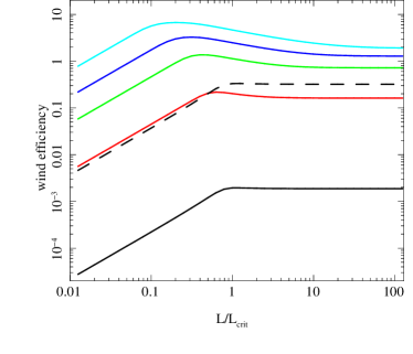
Fig.3 shows the efficiency of wind production, defined as the ratio of mass loss rate in the wind to the mass accretion rate required to produce the wind (which is $\propto L$). We show this efficiency as a function of $L/L_{crit}$ for different disc sizes, with $R_{out}=0.1R_{IC}$ (black), $0.3R_{IC}$ (red) $1R_{IC}$ (green), $3R_{IC}$ (blue), and $10R_{IC}$ (cyan). For large discs, there is a clear change in behaviour from constant efficiency (wind mass loss rate scaling with $L$, region A) at high $L/L_{crit}$ to increasing efficiency at lower $L/L_{crit}$ (wind mass loss rate scaling with $L^{2/3}$ in region B) for $L_{min}<L<L_{crit}$ before the steep decline in efficiency for $L<L_{min}$ (region C, see (blue) vertical line in Fig. 1 for $R_{out}=10R_{IC}$). Thus the minimum luminosity to produce an efficient wind is $L_{min}=L_{crit}(R_{IC}/R_{out})$ (low Compton temperature) rather than $L>L_{crit}$. Most of the wind is launched from the outer disc (see Fig.2b) so the minimum requirement for a wind is that the outer radii of the disc are in region B, rather than that the wind extends down to $R_{IC}$.

Thus thermal winds are predicted to be strongest in the systems with largest discs. This reflects the observed distribution. Winds are preferentially seen from systems with the longest orbital periods i.e. the systems with the largest discs (Diaz-Trigo & Boirin 2016). It is highly unlikely that a magnetic wind would depend on the outer disc size, so this alone favours a thermal wind origin to explain the observed data.

Instead, for a small disc with $R_{out}\ll R_{IC}$ the wind changes from constant but low efficiency (exponential scale height atmosphere with isothermal temperature, region E) to being strongly suppressed by inefficient heating in region D (red vertical line in Fig. 1 for a disc with $R_{out}=0.1R_{IC}$).

Figure 4: a) The dashed line/open circles show the column density in the wind (excluding the static corona) as a function of cosine of the inclination angle from the hydrodynamic simulations of W96 for $T_{IC,8}=0.13$ for pairs of $L/L_{Edd},R_{out}$ of $0.01,12$ (black) $0.08,5$, (red) and $0.3,5$ (green). The solid lines show the columns resulting for each of these from the analytic approximations assuming that the density is $\propto(1-\cos(i))$ and that the typical velocity of the wind is the average (mass loss weighted) sound speed. This is $\sim 140,350$ and $420$ km/s for each of the simulations, respectively. The very simple analytic approximations agree with the results of the hydrodynamic simulations to within a factor $\sim 1.5-2$ over a broad range of angles. b) The ionisation parameter of the wind. This decreases at higher inclination (lower $\cos(i)$) as the density in the wind is higher.

The wind efficiency is larger than unity for all discs with $R_{out}>R_{IC}$ and $L>L_{min}$, showing how powerful these winds can be. This is a feature of thermal winds which was stressed in the early papers, that they can remove more mass than is required to keep the source bright enough to power the wind (B83). Shields et al (1986) showed that these strong wind losses could cause oscillations in an otherwise steady state disc. However, most black hole binaries, especially those with large discs, are unstable to the hydrogen ionisation disc instability (see e.g. Lasota 2001). Thus the strongest wind losses are not likely to be in stable disc systems. Instead, the wind mass loss should impact on the length of the outburst in transient black hole binary sources, as noted by Dubus et al (2001).

B83 comment that the mass loss rates are probably underestimated for the smallest disc sizes ($R_{out}<R_{IC}$) due to the changing streamline pattern that results from not having an outer disc wind to collimate the flow from the inner regions. They suggest that this leads to an increase in the wind mass loss rate by a factor $1/\zeta^{2}$. We show the effect of this for the lowest $R_{out}=0.1R_{IC}$ (i.e. $\zeta\leq 0.1$) as the dashed black line in Fig.3. Plainly, this correction has a very large impact on the mass loss rate predictions from small discs, but it is highly uncertain as there are no hydrodynamical simulations in this regime. Hence we do not consider this further here.

2.1 Predicting the absorption structures

Fig.3 shows that the thermal wind drops dramatically when the luminosity drops below the minimum required to heat the material on the outer disc to the escape velocity. This minimum luminosity is a few percent of the Eddington limit for $T_{IC,8}=1.0$ for a disc with $R_{out}\sim R_{IC}$. Co-incidentally, this is also the point at which the accretion flow makes its dramatic transition from a soft (disc dominated) to a hard (Compton dominated) spectrum. Thus it is possible that the loss of the wind in the hard state is simply a consequence of the lower luminosity in this state leading to a heating rate which is not sufficient for the wind to reach its Compton temperature. However, the large spectral change also means that there is a large change in Compton temperature, with the hard spectrum having larger $T_{IC}$, so $L_{crit}$ and $R_{IC}$ both go down. This illustrates the difficulty with understanding how the wind responds when the equations are written in terms of variable parameters $R_{IC}$ and $L_{crit}$ which depend implicitly on $T_{IC}$ rather than absolute $L$ and $R$.

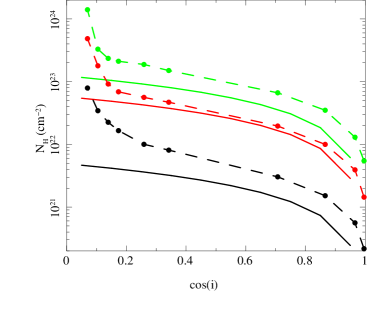
The key observables are the column density in the wind, and its ionisation state. The velocity is also another potential observable but this requires excellent spectral resolution to accurately determine the low velocities expected from an outflow from the outer disc. These are currently only accessible using the Chandra HETGS (especially the 3rd order grating data: Miller et al 2015), but should become much better determined in the future with calorimeter resolution. To derive these observables from the models really requires the full information on the wind density and velocity as a function of height at all radii. This is beyond the scope of the analytic equations discussed above. However, these are included in the hydrodynamic simulations of W96, and they show column as a function of angle for three of their simulations for $L/L_{Edd}=0.3,0.08$ and $0.01$ for fixed illuminating spectrum with $T_{IC,8}=0.13$ and disc $R_{out}=5R_{IC}$ (except for $L/L_{Edd}=0.01$, where $R_{out}=12R_{IC}$: Woods, private communication). W96 give the total column (their tables 2-4), but this includes the column density from the static corona region as well as the wind, whereas our mass loss rates are (by definition) for the wind alone. Hence we use their estimate for the fraction of the column which arises in the static corona (below the softening radius) to derive the column from the wind material in order to compare with the analytic equations. The resulting wind column depends on inclination angle, $i$, which can be approximately described as $N_{H}(i)\propto(1-\cos(i))$ for all angles which do not intersect the disc photosphere itself.

We make the highly simplified assumptions that the velocity is constant, given by the mass loss weighted average sound speed. This gives $v_{out}$ of $\sim 140,350$ and $420$ km/s for $L/L_{Edd}=0.01,0.08$ and $0.3$, respectively. We also define an inner radius for effective launching of the wind i.e. $R_{in}=0.2R_{IC}$ for $L\geq L_{crit}$ (Region A) and $R_{in}=0.2R_{IC}/(L/L_{crit})$ for $L<L_{crit}$ (using the low temperature prescription for Region B according to W96 rather than B83, dashed line in Fig. 1). We assume that the wind streamlines are radial, that $n(R,\cos(i))=n_{0}(R)(1-\cos(i))$, and use mass conservation to fix the edge-on density $n_{0}(R)=\dot{M}/(4\pi R^{2}v_{out}m_{i})$. This gives a column of

$$N_{H}(i)=\int_{R_{in}}^{R_{out}}n_{0}(R)(1-\cos(i))dR=\frac{\dot{M}(1-\cos(i))}{4\pi R_{in}v_{out}m_{i}}$$ (6)

We show this prediction (solid lines) overlaid on the hydrodynamic wind results of W96 (points joined by dashed lines) in Fig.4, using their assumed parameters ($T_{IC,8}=0.13$, $M=10^{8}M_{\odot}$ and $R_{out}=5R_{IC}=7.5\times 10^{18}$ cm, or $12R_{IC}$ for $L/L_{Edd}=0.01$). Our results are within a factor of 2 of the hydrodynamic simulations, which is a remarkable match given the simplistic assumptions.

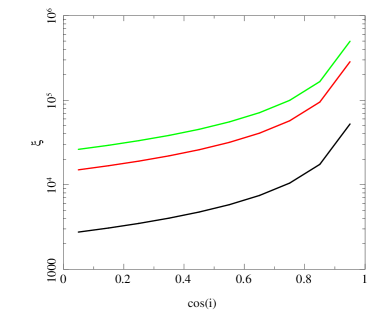
The standard photon ionisation parameter $\xi=L_{ion}/(nR^{2})$, where $L_{ion}$ is the ionising luminosity $\approx L$ for black hole binaries as almost all the luminosity is emitted above 13.6 eV. The ionisation parameter is constant along the radial streamlines, given by

$$\xi(i)=\frac{4\pi m_{i}v_{out}L}{\dot{M}(1-\cos(i))}$$ (7)

Hence the ionisation state is lower close to the orbital plane ($\cos(i)=0$), where the density of the wind is higher, and lower for lower luminosity. These are shown in Fig. 4b.

Thus the thermal wind models can predict not only the overall mass loss rate from the disc, but also the zeroth order observables of column density, and mean ionisation state and velocity along any sightline for any disc size, luminosity and for any radiation spectrum. However, current data (e.g. Miller et al 2015) already give better resolution on the structure of these winds than our simplistic, single zone model, and we stress that full hydrodynamic simulations of thermal winds are required for a detailed comparison.

3 Evolution of the wind with $L/L_{Edd}$

Most black hole binaries are transient, showing outbursts in which the mass accretion rate onto the central object changes dramatically due to the Hydrogen ionisation disc instability (see e.g. the review by Lasota 2010). There is an abrupt transition in spectral state on the fast rise from a hard spectrum which can be roughly described by a power law with photon index $\sim 1.6-2$, to a much softer spectrum which is dominated by a multi-colour disc component. This hard to soft transition is not at a well defined luminosity, most probably because the mass accretion rate is changing too rapidly for the disc to be in steady state (Smith et al 2002; Gladstone, Done & Gierlinski 2007). Instead, the slow decline is more stable, with the spectrum changing back from a disc to power law spectrum at $L\sim 0.02L_{Edd}$ (Maccarone 2003). During the disc dominated, most luminous phase, the characteristic disc temperature is $kT_{max}\propto(L/L_{Edd})^{1/4}$. The outer disc sees this at high inclination, so the Doppler blueshift increases the temperature seen by the disc. We model a $10M_{\odot}$ black hole with spin $a_{*}=0.5$ using the kerrbb code in xspec which has full general relativistic emissivity and ray tracing. Assuming a mass accretion rate of $3.5\times 10^{17}$ g s^-1 ($L/L_{Edd}\sim 0.02$), with a colour temperature correction of $f_{col}=1.7$, the outer disc sees a spectrum similar to a multicolour disc blackbody with maximum temperature of $0.6$ keV, which corresponds to $kT_{IC}=0.31$ keV which is $0.036\times 10^{8}$ K. Hence this predicts that in the disc dominated spectra,

$$T_{IC,8}=0.036[L/(0.02L_{Edd})]^{1/4}$$ (8)

The transition to the hard state is complex, with the disc temperature decreasing rapidly, as expected if the thin disc starts to recede from the innermost stable circular orbit (e.g. Gierlinski, Done & Page 2008). Here we assume that the spectrum abruptly changes to a power law of photon index $\Gamma=2$ at $L=0.02L_{Edd}$, flattening to $\Gamma=1.6$ at $L/L_{Edd}=2\times 10^{-3}$. Interpolating logarithmically $\Gamma=1.6+0.4\times\log_{10}[L/(0.002L_{Edd})]$. The Compton temperature for a hard power law depends on the high energy cutoff, but this dependence saturates above 100 keV due to the rollover in the Klein-Nishima cross-section compared to the constant cross-section assumed in Thomson scattering. Hence we fix the upper limit of the flux integral at 100 keV, and assume a lower limit of 0.1 keV. This gives an inverse Compton temperature of 3.6 keV ($0.42\times 10^{8}$ K), increasing to 7.6 keV ($0.88\times 10^{8}$ K) for the hardest spectra/lowest luminosities considered here, so that

$$T_{IC,8}=0.88-0.46\times\log_{10}[L/0.002L_{Edd}]$$ (9)

We use this correlated change in $kT_{IC}$ with $L/L_{Edd}$ to explore the predicted wind behaviour over the range $10^{-3}L_{Edd}<L<L_{Edd}$, with the total mass loss rate in the wind $\dot{M}$ calculated from the fitting formulae of W96 and the column/ionisation state observables approximated as in Section 2 above. We assume a generic black hole of mass $M=10M_{\odot}$ and set the disc outer radius to $3.7\times 10^{12}$ cm ($2.5\times 10^{6}R_{g}$, which corresponds to $5R_{IC}$ for $T_{IC,8}=0.13$ as used in most of the simulations in W96). We note that most BHB have much smaller discs, but the most dramatic winds are indeed seen in systems which are known to be in long period orbits (GRS1915+105, GRO J1655-40), or where the orbital periods are unknown but consistent with being long (H1743-322, 4U1630-522) e.g. Diaz Trigo & Boirin (2016).

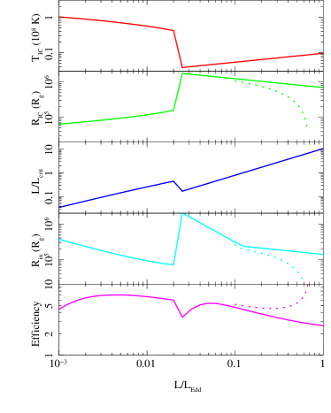
The upper panel of Fig. 5 shows the Compton temperature as a function of $L/L_{Edd}$, illustrating the dramatic change in behaviour at the hard/soft spectral transition at $L\sim 0.02L_{Edd}$. This has a similarly dramatic impact on the radius at which Compton temperature allows material to escape, $R_{IC}$, shown as the solid line in the second panel of Fig. 5. However, the effective launch radius, $R_{in}$, depends on luminosity relative to the critical luminosity which is required to launch the wind efficiently, which itself depends on $T_{IC}$. The third panel in Fig. 5 shows $L/L_{crit}$. This only reaches unity for $L>0.1L_{Edd}$, so only above this luminosity is $R_{in}=0.2R_{IC}$ (fourth panel, Fig. 5). Below this, $R_{in}=0.2R_{IC}/(L/L_{crit})$ so it decreases with increasing luminosity in the low/hard state, as well as showing more complex behaviour at the transition due to the jump in Compton temperature. However, all of these are within the disc outer radius, so the outer parts of the disc are in the strong wind region B even for $L/L_{crit}<1$. The final panel shows the wind efficiency i.e. the ratio of mass loss rate in the wind with the mass accretion rate required to produce the assumed luminosity. This is fairly constant as the outer disc is always in one of the strong wind regions, and high at $\sim 5\times$ the input mass accretion rate. This is a little larger than in the simulations in W96 and Fig. 3 as we are assuming a black hole with spin $0.5$ rather than spin 0, so the same luminosity is produced with a lower mass accretion rate.

Figure 5: The upper panel shows the assumed change in $T_{IC}$ with $L/L_{Edd}$ (red). The power law spectral index softens with increasing luminosity in the low/hard state, so the inverse Compton temperature drops. The abrupt drop at $L/L_{Edd}=0.02$ marks the transition to the disk dominated state, where the Compton temperature increases with luminosity. The second panel shows the effect of this on $R_{IC}$ (green). A higher Compton temperature means that the wind can escape from smaller radii. The third panel shows how $L/L_{crit}$ changes (blue). An increase in Compton temperature means that the radiation heats the gas faster, so it can drive the temperature up to $T_{IC}$ at $R_{IC}$ at a lower luminosity. The assumed $L/L_{Edd}-T_{IC}$ behaviour means that the luminosity is only above the critical luminosity for $L>0.1L_{Edd}$. Thus the wind is lauched from $R_{in}=0.2R_{IC}$ only for $L>0.1L_{Edd}$. Below this, the wind instead is launched from $R_{in}=0.2R_{IC}/(L/L_{crit})$, so the wind launch radius (cyan) decreases with increasing $L/L_{Edd}$ in the low/hard state, as the increase in $L/L_{crit}$ more than offsets the increase in $R_{IC}$. The lower panel (magenta) shows the wind efficiency (mass outflow rate in terms of the mass accretion rate). This is fairly constant at $\sim 5\times$ the mass accretion rate required to produce the luminosity, except for more complex behaviour around the transition. The dotted lines on all panels show the effect of including a simple radiation pressure term to reduce the effective gravity. The wind can be launched from progressively smaller radii, and the mass loss rates increase.

4 Radiation pressure correction

Neither B83 nor W96 include radiation pressure on electrons in their hydrodynamic simulations. However, this must become important as $L\to L_{Edd}$. By definition, static material above the disc will be driven out as a wind at $L>L_{Edd}$, as the radiation pressure reduces the effective gravity to $GM/R^{2}(1-L/L_{Edd})$. However, the wind material is not static as it has the Keplarian rotation velocity from where it was launched as well as thermal motion driven by the pressure gradients. This will mean that it becomes unbound at all radii at luminosities somewhat below $L_{Edd}$. A lower limit to this completely unbound luminosity is $L_{Edd}/2$, which could be reached if all the Keplarian azimuthal rotational velocity ($v_{\phi}=v_{esc}/\sqrt{2}$) were converted to radially outward velocity (Ueda et al 2004). Conserving angular momentum as well as energy pushes this up to $L_{Edd}/\sqrt{2}$. This is very close to the results of a full calculation in Proga & Kallman (2002). In the case where the disc luminosity at the wind launch radius is negligible, they show (equations 20-22) that the effective gravity goes to zero at $H\sim R$ for $L\sim L_{Edd}/(1+\pi/8)\approx L_{Edd}/\sqrt{2}$. This gives a simple correction to the Compton radius of

$$\overline{R}_{IC}\approx R_{IC}\Bigl{(}1-\frac{L}{0.71L_{Edd}}\Bigr{)}$$ (10)

We first assume that this correction to the inverse Compton radius, $\overline{R}_{IC}$, is the only change in wind properties, and rerun the black hole binary simulation. The new results are shown as the dotted lines on Fig. 5. The lower effective gravity as the luminosity increases towards Eddington means that $R_{IC}$ and hence $R_{in}$ both decrease dramatically, formally going to zero at $0.71L_{Edd}$ (dashed green and cyan lines in the second and fourth panels). The wind can then be launched from everywhere on the disc, so the mass loss rates also increase. We note that this is likely to be an underestimate of the increase in mass loss rate as we still assume that the wind velocity is given by the sound speed, but it should be higher due to the contribution of radiaton pressure to the acceleration.

Figure 6: The upper panel (red) shows the column density at $\cos(i)=0.25$ i.e. an inclination angle of $\sim 75^{\circ}$. This is roughly proportional to the mass accretion rate, but with a dip at the spectral transition due to the lower Compton temperature of the dimmest high/soft states. The second panel (green) shows the ionisation state calculated from the total bolometric flux, $\xi=L_{bol}/nR^{2}$. This is fairly constant, as the increase in luminosity is mostly balanced by an increase in density of the wind. The third panel shows the fraction of bolometric flux which is emitted in the 8.8-30 keV high energy bandpass (blue). These are the photons which are most effective in photoionising He- and H-like iron, and this shows a dramatic dip around the spectral transition, even including a power law to higher energies which carries 5% of the total disc luminosity. The fourth panel shows the high energy ionisation parameter, $\xi_{H}=f_{H}L_{bol}/nR^{2}$ (cyan). This is almost completely constant in the low/hard state, but dips dramatically in the high/soft state due to the much softer spectra, and only recovers to the same value as seen in the low/hard state at the highest luminosities. The bottom panel shows the outflow velocity. This mirrors the behaviour of the launch radius of the wind shown in Fig.5d. The dashed lines show the effect of including a simple radiation pressure correction. The wind becomes optically thick ($N_{H}>2\times 10^{24}$ cm^-2, and has much lower ionisation parameter around $L\sim 0.7L_{Edd}$, as required to explain the dramatic wind in GRO J1655-40 (Miller et al 2006, Shidatsu et al 2016).

5 Predicted absorption features

5.1 Behaviour at the transition

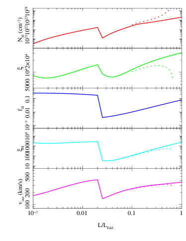
We calculate the observable features of the simple model for the BHB spectral evolution as a function of $L/L_{Edd}$ introduced in the previous sections. Fig.6 shows the observables of $N_{H}$ (upper panel, red) and $\xi$ (middle panel, green), extracted for an inclination of $75^{\circ}$ ($\cos(i)=0.25$). The solid lines show the standard thermal wind model results. The column density is roughly proportional to mass accretion rate, but with a drop at the spectral transition due to the large change in spectral shape changing the Compton radius and critical luminosity. This predicts that there should be an abrupt increase in column by around a factor 10 as the source declines and makes the transition to the low/hard state. This is exactly opposite to the claimed behaviour of the wind shutting off in the low/hard state.

However, the visibility of the wind is also controlled by its ionisation state. The ionisation parameter calculated from the full luminosity, $\xi=L/(nR^{2})$, is almost constant, changing only by a factor 5 as the luminosity varies by a factor of a thousand. This is because the ionisation is roughly proportional to ratio of luminosity and wind mass loss rate (equation 7) so these cancel in the regime where the wind efficiency is roughly constant. However, the photo-ionisation of iron depends on the high energy 8.8-30 keV flux, which changes dramatically at the transition. This high energy flux would be very small for the lowest luminosity high/soft states as these have low temperature discs with very few photons emitted above 8.8 keV. However, such pure disc spectra are rare. Most high/soft states have a small, soft power law tail giving some higher energy flux. Hence we also include an additional power law in the high/soft state, with index fixed at $\Gamma=2.2$, which carries 5% of the total power. This has little impact on the Compton temperature, but will determine the photo-ionisation of iron ions. The third panel in Fig.6 (blue) shows the fraction of the bolometric flux which is emitted in the high energy 8.8-30 keV bandpass, $f_{H}$, while the fourth panel (cyan) shows the corresponding high energy photoionisation parameter, $\xi_{H}=f_{H}L/(nR^{2})=f_{H}\xi$. This drops by a factor of more than 50 at the transition, so the photo-ionisation of the wind changes dramatically.

However, the baseline ion population of iron is set by collisional ionisation rather than photo-ionisation - the wind is heated to a temperature $T_{ch}$, so the ion populations cannot drop below those which characterise material at this temperature. We will explore this in detail in a subsequent paper, but here we just note that neither the Compton temperature nor the high energy photo-ionisation parameter are high enough to completely strip iron in the wind in the low/hard state. Thus while there is a large change in ion populations in the wind across the transition, it is not likely that this is the origin of the lack of iron absorption features in the wind in the low/hard state (Neilsen & Lee 2009; Miller et al 2012).

5.1.1 Comparison to observations across the transition

We analyse the constraints from the data across the transition in more detail. The observations of Neilsen & Lee (2009) are of GRS1915+105, a source which is close to its Eddington limit, even in its hardest spectral states, which is a hard intermediate state rather than a true low/hard state (Done, Wardzinski & Gierlinski 2004). Hence this requires more detailed modelling which will be the subject of a later paper (Shidatsu et al, in preparation). However, the observations of H1743-322 of Miller et al (2012) are in standard low/hard and high/soft states which are directly comparable to those simulated in the previous section. Hence we can use our models to directly compare to the observed thermal wind features across the spectral transition.

Figure 7: The low/hard (black) and high/soft (red) spectra from RXTE data on H1743-322, with the inset showing the simultaneous Chandra data, with a clear difference in wind absorption features. The high energy 8.8-30 keV photo-ionising flux is quite similar between the two datasets, but the overall luminosity is quite different. If the wind stayed constant, responding only to the high energy photo-ionising flux, then the difference in wind properties would require a change in the wind structure, potentially linked to the appearance of the jet. However, thermal winds respond to the overall flux, as well as to the high energy part, and this predicts that the column should be smaller by a factor of $\sim 5$ in the low/hard state, consistent with the observations.

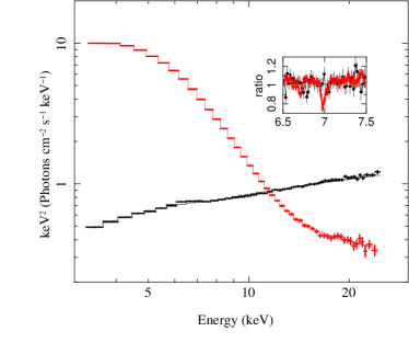We extract the simultaneous RXTE/Chandra data for these observations in order to constrain the continuum shape and luminosity as well as the wind features. The standard pipeline RXTE continuum spectra are shown in Fig.7 (ObsIDs P95368-01-01-00 and P80135-02-01-11 for the low/hard and high/soft states, respectively), with the inset showing the TGCAT coadded HEG $\pm$ 1 Chandra high resolution spectra (ObsIDs 3803 and 11048, respectively) around the iron line bandpass. It is obvious that there is a large change in bolometric luminosity as well as the state change and the change in wind absorption features. The wind should clearly have higher column in this particular high/soft state than the comparison low/hard state simply because the source has higher bolometric luminosity (see Fig.5e and 6a).

Integrating the model to get an unabsorbed bolometric flux gives $9.7\times 10^{-9}$ ergs s^-1 cm^-2 for the low/hard state using the nthcomp model with an assumed electron temperature of 100 keV, while the diskbb model for the high/soft state gives $4.3\times 10^{-8}$ ergs s^-1 cm^-2. However, the intrinsic luminosity of the high/soft state is probably higher due to projection effects as the disc is seen at high inclination - as evidenced by the fact it has a disc wind (Ponti et al 2012) and a strong low frequency QPO (Ingram et al 2016) as well as a high temperature disc (Munoz Darias et al 2013). The system parameters are not well known, but Dunn et al (2010) show the hardness-intensity diagram for the outbursts look similar to those of other BHB for a canonical 10M_⊙ mass and 5 kpc distance. This then gives $L/L_{Edd}=0.02$ (low/hard) and $0.1$ (high/soft) without any projected area correction, or $L/L_{Edd}\sim 0.4$ with a cosine dependence assuming $i\sim 75^{\circ}$ (Steiner et al 2012). This fits rather well with the observed spectrum, as the diskbb temperature is 1.2 keV, i.e. $2\times$ higher than that assumed at the transition at $L/L_{Edd}=0.02$, so the luminosity should be $2^{4}=16\times$ higher, at $L/L_{Edd}\sim 0.3$. The tail in the high/soft state carries roughly 5% of the total bolometric power, so these two spectra are very comparable to those assumed in the simulations shown in Figs.5 and 6.

The thermal wind model then predicts that there should be a wind column of $\sim 8\times 10^{22}$ cm^-2 in the high/soft state, a factor 5 larger than the predicted column of $1.6\times 10^{22}$ cm^-2 in the low/hard state. This is despite the fact that the high energy luminosities are similar in the low/hard and high/soft states. Thermal winds respond to changes in total luminosity and spectral shape and are not just dependent on the high energy photo-ionising flux. The models predict that the high energy photo-ionisation parameter is lower by a factor 5 in the high/soft state, as there is a stronger wind, but with similar high energy flux. However, this photo-ionisation is not sufficient to fully strip the wind in the low/hard state, so the clear prediction of the thermal wind model is that the absorption features should be $\sim 5\times$ bigger in the high/soft state at $L/L_{Edd}=0.3-0.4$ compared to the brightest low/hard state at $L/L_{Edd}=0.02$, despite them having similar high energy fluxes. This is easily compatible with the Miller et al (2012) results.

5.2 High luminosities and the wind in GRO J1655-40

The dotted lines on Fig.6 show the effect of the simple radiation pressure correction (see Section 4). The column increases dramatically as $L\to 0.7L_{Edd}$, becoming optically thick to electron scattering, with a corresponding drop in ionisation state. The dotted lines on Fig.5 show that this much stronger wind is launched from progressively smaller radii.

Our assumed disc dominated spectra at high luminosity are too simple to describe those seen from GRS1915+105, so here we concentrate only on the comparison to GRO J1655-40, which had a very soft spectrum at the time when it produced the most extreme wind seen from this or any other black hole binary. This anomolous wind has large column, $\log N_{h}\sim 23.8$ and (compared to other binary winds) low ionisation state, $\log\xi=4$ (Miller et al 2006; Miller et al 2008; Kallman et al 2009). This ionisation state is comparable to those predicted here for the simple radiation pressure correction at $L\to 0.7L_{Edd}$, but the observed column is not optically thick, and the observed luminosity is only $\sim 0.05L_{Edd}$ (Miller et al 2006; Miller et al 2008; Kallman et al 2009).

Nonetheless, it seems possible that this could still be at least partly (there are multiple velocity components: Kallman et al 2009; Miller et al 2015; 2016) due to a thermal-radiative wind. The true source luminosity will be underestimated if the wind become optically thick and this optically thick material could be hidden by being completely ionised, with the observed absorption lines arising from an outer thin skin of partially ionised material. In this picture, an optically thick wind is launched by thermal-radiative driving from the inner disc, and expands outwards. Electron scattering in the completely ionised, optically thick material reduces the observed X-ray flux along the line of sight, with the observed absorption lines arising in an outer, optically thin, photosphere of the wind. The detection of the metastable FeXXII shows that this photosphere must have $n\sim 10^{15}$ cm^-3 (Miller et al 2008; Kallman et al 2009) and it is illuminated by the same (supressed) continuum which we see as it is along the line of sight. Hence the observed $\log\xi=4$ implies a position for this photosphere at $R\sim 8\times 10^{8}$ cm ($\equiv 800R_{g}$), as in the magnetic wind models. The difference in this thermal-radiative picture is that the wind is actually launched from even closer to the black hole, and we see only the outer shell of the expanding optically thick material.

This may seen an unnecessarily complex picture given the success of the magnetic wind models in fitting the data quantatively (e.g. Fukumura et al 2017). However, while the magnetic models can quantatitively fit to the observed optically thin wind with the observed low luminosity, they do not explain why this wind is only seen in this one observation of GRO J1655-40. There are other similarly low luminosity Chandra datasets from this source which show much higher ionisation winds, consistent with a thermal driving (Nielsen & Homan 2012), and similarly low luminosity Chandra data from other sources which show only the expected thermal wind signatures of H- and He-like iron (e.g. Ponti et al 2012). The magnetic wind model also does not explain the other unusual features of GRO J1655-40 in this dataset, namely the unusual lack of variability seen in the corona of this state (Uttley & Klein-Wolt 2015), or its unusually steep spectrum (Neilsen & Homan 2012), or give a geometry where the absorption lines only partially cover the source (Kallman et al 2009). By contrast, all these other features can be explained fairly naturally in an optically thick wind model. Downscattering in the wind steepens the spectrum, supresses variability, and makes an extended source geometry for partial covering, and it is rare for BHB to reach (or exceed) Eddington which explains why this wind has such different properties.

Nontheless, a thermal-radiative wind from a source with $L\to L_{Edd}$ remains a speculative explanation for this observation of GRO J1655-40. To test whether this scenario can work quantatively requires a hydrodynamic code to calculate the two dimensional wind structure, including radiative continuum driving (e.g. Proga & Kallman 2004) with full Monte- Carlo radiation transport to handle the scattered flux (e.g. Higgingbottom et al 2014). However, the limitations of the magnetic wind models in explaining why the wind in this observation of GRO J1655-40 is so different from other observations of this and other BHB’s motivate consideration of the possibility.

6 Conclusions

We use the analytic models for thermal winds of B83 and W96, combined with a very simple geometric/kinematic model for the structure of the wind to predict the column density, ionisation and velocity along any line of sight at any luminosity for any spectrum. We combine this with a very simple model of the spectral evolution with luminosity in BHB, including the major change in Compton temperature at the hard-soft spectral transition, as well as the smaller but systematic change in Compton temperature with luminosity within each state.

We show that the column density of the wind seen at any luminosity generally increases with increasing mass accretion rate except for a dip just after the transition to the high/soft state, where the much lower Compton temperature suppresses the wind. This predicts that there is more wind material just after the source makes a transition to the low/hard state, in direct contrast to claims that the wind is suppressed in the low/hard state and seen only in the high/soft state. While photo-ionisation also plays a role in the visibility of the wind, we show that this is probably not enough to supress a wind just after the transition to the low/hard state if it was visible in the high/soft state just beforehand.

We critically examine the data on which the claims of wind suppression are based. GRS1915+105 (Neilsen & Lee 2009) is close to Eddington, and has complex spectra so the very simple models used here are probably not applicable. Instead, H1743-322 (Miller et al 2012) shows cannonical low/hard and high/soft states, with Chandra data clearly showing that the wind in the high/soft state is absent in low/hard data with similar high energy luminosity. However, these two spectra are very different in total luminosity, and this difference is enhanced by the cosine dependence of the disc flux in the high/soft state, while the low/hard state emission is more isotropic. We estimate that these two spectra differ by an order of magnitude in intrinsic luminosity, so the much stronger wind in the high/soft state is entirely in line with the thermal wind predictions.

This removes any need for suppression of the wind at the transition via magnetic fields switching from powering the wind in the high/soft state, to powering the jet in the low/hard state (Neilsen & Lee 2009). Indeed, such a switch would be very surprising, as the jet is almost certainly launched from the inner disc, while the low outflow velocities seen in the wind shows that it is most likely launched from the outer disc.

Radiation pressure should become important as the source approaches the Eddington limit, increasing the mass loss rate as material above the disc is unbound at progressively smaller radii. We include a simple correction for this which predicts stronger winds launched from smaller radii as $L\to L_{Edd}$. This may be able to explain the anomolous wind seen in GRO J1655-40 (Miller et al 2006) if the wind becomes optically thick, supressing the observed luminosity (Shidatsu et al 2016). However, a quantative comparison requires hydrodynamic simulations in the Eddington regime which are beyond the scope of this paper. Alternatively, Fukumura et al (2017) have shown quantatatively that magnetic driving can be consistent with the broad properties of this anomlous wind, though their model does not explain why similar winds are not seen in this or other BHB at similar luminosities, nor does it address the likelihood of the required magnetic field configuration.

We conclude that there is at present no strong requirement for magnetic winds in the majority of BHB, and it is possible that they are not required in the supermassive black holes either (e.g Hagino et al 2015; 2016). Known wind launching mechanisms (thermal, UV line driven and Eddington continuum) should be explored in detail before ruling them out in favour of magnetic winds.

References

- [Begelman et al.(1983)] Begelman, M. C., McKee, C. F., & Shields, G. A. 1983, ApJ, 271, 70
- [Chakravorty et al.(2013)] Chakravorty, S., Lee, J. C., & Neilsen, J. 2013, MNRAS, 436, 560
- [Díaz Trigo & Boirin(2013)] Díaz Trigo, M., & Boirin, L. 2013, Acta Polytechnica, 53, 659
- [Díaz Trigo et al.(2014)] Díaz Trigo, M., Migliari, S., Miller-Jones, J. C. A., & Guainazzi, M. 2014, A& A, 571, A76
- [Díaz Trigo & Boirin(2016)] Díaz Trigo, M., & Boirin, L. 2016, Astronomische Nachrichten, 337, 368
- [Done et al.(2004)] Done, C., Wardziński, G., & Gierliński, M. 2004, MNRAS, 349, 393
- [Done et al.(2007)] Done, C., Gierliński, M., & Kubota, A. 2007, A& A Rev, 15, 1
- [Done(2010)] Done, C. 2010, arXiv:1008.2287
- [Dubus et al.(2001)] Dubus, G., Hameury, J.-M., & Lasota, J.-P. 2001, A& A, 373, 251
- [Fukumura et al.(2017)] Fukumura, K., Kazanas, D., Shrader, C., et al. 2017, Nature Astronomy, 1, 0062
- [Gierliński et al.(2008)] Gierliński, M., Done, C., & Page, K. 2008, MNRAS, 388, 753
- [Gladstone et al.(2007)] Gladstone, J., Done, C., & Gierliński, M. 2007, MNRAS, 378, 13
- [Hagino et al.(2015)] Hagino, K., Odaka, H., Done, C., et al. 2015, MNRAS, 446, 663
- [Hagino et al.(2016)] Hagino, K., Done, C., Odaka, H., Watanabe, S., & Takahashi, T. 2016, arXiv:1611.00512
- [Higginbottom & Proga(2015)] Higginbottom, N., & Proga, D. 2015, ApJ, 807, 107
- [Higginbottom et al.(2014)] Higginbottom, N., Proga, D., Knigge, C., et al. 2014, ApJ, 789, 19
- [Ingram et al.(2016)] Ingram, A., van der Klis, M., Middleton, M., et al. 2016, MNRAS, 461, 1967
- [Jimenez-Garate et al.(2002)] Jimenez-Garate, M. A., Raymond, J. C., & Liedahl, D. A. 2002, ApJ, 581, 1297
- [Kalemci et al.(2016)] Kalemci, E., Begelman, M. C., Maccarone, T. J., et al. 2016, MNRAS, 463, 615
- [Krolik et al.(1981)] Krolik, J. H., McKee, C. F., & Tarter, C. B. 1981, ApJ, 249, 422
- [Kubota et al.(2007)] Kubota, A., Dotani, T., Cottam, J., et al. 2007, PASJ, 59, 185
- [Lasota(2001)] Lasota, J.-P. 2001, New Astronomy Reviews, 45, 449
- [Luketic et al.(2010)] Luketic, S., Proga, D., Kallman, T. R., Raymond, J. C., & Miller, J. M. 2010, ApJ, 719, 515
- [Maccarone(2003)] Maccarone, T. J. 2003, A& A, 409, 697
- [Miller et al.(2006)] Miller, J. M., Raymond, J., Fabian, A., et al. 2006, Nature, 441, 953
- [Miller et al.(2012)] Miller, J. M., Raymond, J., Fabian, A. C., et al. 2012, ApJL, 759, L6
- [Miller et al.(2015)] Miller, J. M., Fabian, A. C., Kaastra, J., et al. 2015, ApJ, 814, 87
- [Miller et al.(2016)] Miller, J. M., Raymond, J., Fabian, A. C., et al. 2016, ApJL, 821, L9
- [Muñoz-Darias et al.(2013)] Muñoz-Darias, T., Coriat, M., Plant, D. S., et al. 2013, MNRAS, 432, 1330
- [Nayakshin et al.(2000)] Nayakshin, S., Kazanas, D., & Kallman, T. R. 2000, ApJ, 537, 833
- [Neilsen & Lee(2009)] Neilsen, J., & Lee, J. C. 2009, Nature, 458, 481
- [Neilsen et al.(2016)] Neilsen, J., Rahoui, F., Homan, J., & Buxton, M. 2016, ApJ, 822, 20
- [Ponti et al.(2012)] Ponti, G., Fender, R. P., Begelman, M. C., et al. 2012, MNRAS, 422, 11
- [Proga & Kallman(2002)] Proga, D., & Kallman, T. R. 2002, ApJ, 565, 455
- [Shidatsu et al.(2016)] Shidatsu, M., Done, C., & Ueda, Y. 2016, ApJ, 823, 159
- [Shields et al.(1986)] Shields, G. A., McKee, C. F., Lin, D. N. C., & Begelman, M. C. 1986, ApJ, 306, 90
- [Smith et al.(2002)] Smith, D. M., Heindl, W. A., & Swank, J. H. 2002, ApJ, 569, 362
- [Steiner et al.(2012)] Steiner, J. F., McClintock, J. E., & Reid, M. J. 2012, ApJL, 745, L7
- [Ueda et al.(2004)] Ueda, Y., Murakami, H., Yamaoka, K., Dotani, T., & Ebi sawa, K. 2004, ApJ, 609, 325
- [Ueda et al.(2010)] Ueda, Y., Honda, K., Takahashi, H., et al. 2010, ApJ, 713, 257
- [Uttley & Klein-Wolt(2015)] Uttley, P., & Klein-Wolt, M. 2015, MNRAS, 451, 475
- [van Paradijs & McClintock(1994)] van Paradijs, J., & McClintock, J. E. 1994, A& A, 290, 133
- [Woods et al.(1996)] Woods, D. T., Klein, R. I., Castor, J. I., McKee, C. F., & Bell, J. B. 1996, ApJ, 461, 767
- [Zoghbi et al.(2016)] Zoghbi, A., Miller, J. M., King, A. L., et al. 2016, ApJ, 833, 165