Measure the Propagation of a halo CME and Its Driven Shock with the Observations from a Single Perspective at Earth
Abstract
We present a detailed study of an earth-directed coronal mass ejection (Full halo CME) event happened on 2011 February 15 making use of white light observations by three coronagraphs and radio observations by Wind/WAVES. We applied three different methods to reconstruct the propagation direction and traveling distance of the CME and its driven shock. We measured the kinematics of the CME leading edge from white light images observed by STEREO A and B, tracked the CME-driven shock using the frequency drift observed by Wind/WAVES together with an interplanetary density model, and obtained the equivalent scattering centers of the CME by Polarization Ratio(PR) method. For the first time, we applied PR method to different features distinguished from LASCO/C2 polarimetric observations and calculated their projections onto white light images observed by STEREO A and B. By combining the graduated cylindrical shell (GCS) forward modeling with the PR method, we proposed a new GCS-PR method to derive 3D parameters of a CME observed from a single perspective at Earth. Comparisons between different methods show a good degree of consistence in the derived 3D results.
Subject headings:
Sun:corona — Sun:corona mass ejections(CMEs) — Sun: radio radiation — solar-terrestrial relations1. Introduction
Coronal Mass Ejections (CMEs) are powerful eruptions that release huge clouds of plasma threaded with magnetic field lines from the Sun into interplanetary space. These events have an influence on the entire near-Sun heliosphere. On Earth they can cause technical problems to power grids, oil pipelines, or telecommunication equipments (Pirjola, 2002). Moreover, high energy particles propelled from these events could be a potential threat to human life in space(Facius & Reitz, 2006). In order to predict the arrival of a CME and avoid potential damages, many methods have been developed to monitor the position and three-dimensional (3D) structure of CMEs using data from multiple coronagraphs. These methods include stereoscopy (Inhester, 2006; Aschwanden et al., 2008), GCS Forward Modeling (GCSFM) (Thernisien et al., 2006), Polarization Ratio method (PR) (Moran & Davila, 2004), mask fitting (Feng et al., 2012), and the local correlation tracking plus triangulation (Mierla et al., 2009). Comparisons between different methods have been made by Mierla et al. (2010), Thernisien (2011) and Feng et al. (2013).
Of particular importance to space weather are the so-called halo CMEs. They propagate in direction close to the Sun-Earth line and have been observed by coronagraphs on board different near-Earth spacecraft such as P78-1, SMM and the SOHO (Domingo et al., 1995). In 2006 the twin STEREO spacecraft were launched to monitor transient events in interplanetary space from two vantage points off the Sun-Earth line, and to determine their 3D locations (Kaiser et al., 2008). The observations from this mission have greatly improved the determination of CME propagation. However, the lifetime of the STEREO mission is limited and currently STEREO-B has only been recovered after an almost two year loss of contact. The state of the instrument is not yet clear. It is therefore of some interest to find out how well we can predict the propagation direction and speed of a halo CME from observations made from a single perspective alone, especially from a near-Earth position. Most future missions equipped with coronagraphs, e.g., ESA’s PROBA-3(Zhukov, 2014), Indian Aditya-L1(Nandi, 2015), and Chinese ASO-S(Gan et al., 2015), will image the inner corona from about 1.1 to 3 from the near-Earth perspective. The other two future missions which will escape Earth, Solar Orbiter and Solar Probe Plus (Velli, 2013), will have highly ecliptic orbits not well suited for a synoptic CME watch. It is therefore not clear to what extent and with which precision we will in the future be able to routinely determine the propagation characteristics of CMEs based on near-Earth observations alone.
The goal of the present paper is to test two methods to analyze halo CME propagation which are independent of the STEREO position geometry. The STEREO data will be used in this paper as a reference to find out how reliable these alternative methods are. One such alternative are characteristic radio burst signals, called type II bursts, usually generated in association with CMEs. Previous studies have shown that type II radio bursts in the decameter to hectometer (DH) and longer wavelength range are produced by CME-driven shocks (Reiner et al., 1998; Bale et al., 1999; Su et al., 2016) and bear signatures which reflect the propagation of the transient events through the interplanetary space (IP space). The observed frequency drift rate can be converted into an approximate velocity of the CME and its shock if a model for the upstream electron density with distance from the Sun is assumed.
However, the source region of the type II radio bursts is still an open question. Gopalswamy (2004) suggested that the type II radio bursts are enhanced and modified due to the interaction between two CMEs. Martínez Oliveros et al. (2012) applied the radio direction-finding technique to an interacting CME event, and compared the results with the white light observations by STEREO from which they concluded that type II radio emission is causally related to the interaction of CMEs. Magdalenić et al. (2014) applied the same technique to another event, and suggested that the interaction between the shock wave and a nearby coronal streamer resulted in the type II radio emission, which is consistent with the conclusion of Shen et al. (2013) .
The PR technique is a second alternative. It was first proposed by Moran & Davila (2004) to convert the polarimetric observations by LASCO/C2 to 3D distances off the plane of the sky (POS), and verified by Dere et al. (2005) using a series of high-cadence (1 hr) LASCO polarization measurements. Later on, Mierla et al. (2009) and Moran et al. (2010) successfully applied this technique to the polarimetric observations from STEREO coronagraphs. The physics behind this method is Thomson scattering and it has been described in detail by Billings (1966) and reviewed by Howard & Tappin (2009) and Inhester (2015). Like the observation of type II radio bursts, the method has the advantage that only the observations from one single perspective is required. Previous studies usually apply this method to limb CMEs where foreground and background contamination of the CMEs is not as severe as for the case of halo CMEs. As halo CMEs are most relevant to geomagnetic storms, we have made efforts to obtain their 3D location with this method by carefully removing other, CME-irrelevant features in the polarimetric observations. For most of the halo CMEs, especially for full halo CMEs, we are lacking the CME observations behind the coronagraph occulter. In order to obtain the 3D CME structure as completely as possible, we also applied the graduated cylindrical shell (GCS) model to fit the halo CME observations and the corresponding 3D points derived with PR method.
In this paper, we select a full halo CME as seen by SOHO. The two STEREO spacecraft were almost in a opposite direction from the Sun and made an angle of about with SOHO. Such a geometry of spacecraft positions simplifies the stereoscopy method and is favorable for comparing the results derived from different methods. In Section 2 we describe the instruments and observations. In Section 3 we present details of analyses methods and their corresponding results. The comparison of the results derived from different methods are shown in Section 4. Section 5 gives a summary of our work.
2. Observations
The CME investigated here was observed on 15 February 2011 from three viewpoints almost simultaneously by the coronagraphs on board the two Solar Terrestrial Relations Observatory (STEREO) (Kaiser et al., 2008) probes and the Solar and Heliospheric Observatory (SOHO) (Domingo et al., 1995) spacecraft. Each of the twin STEREO probes is equipped apart from other instruments with two white-light coronagraphs COR1 and COR2. Their field of view ranges from 1.5 to 4 solar radii and from 2 to 15 solar radii, respectively. The SOHO has two white-light coronagraphs, C2 and C3, on board which together image the solar corona from 2.2 to 30 solar radii(C2: 2.2–6 solar radii, C3: 3.7–30 solar radii)(Brueckner et al., 1995). All of the telescopes can provide polarized and total brightness images.
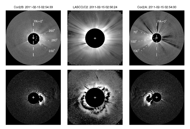
During the period of 13-15 February 2011, there were eight CMEs ejected from the active region AR 11158 as pointed by Maričić et al. (2014). Most of these CMEs were too weak to trace their shape with the desired precision. Therefore, we focus our analysis on a more intense full halo CME, which was first captured by STEREO/COR1 at 01:55UT on 15 February 2011, and was associated with an X2.2 flare. Another reason for us to select this event is the special viewing geometry of the three spacecraft, which gave a full view of the CME from different perspectives. The positions of the three spacecraft during this event are presented in Table 1. The view directions of the STEREO spacecraft almost form a right angle with the view direction of SOHO. Due to this special geometry of the three spacecraft, the CMEs recorded as a halo CME by SOHO was observed as a limb event by both STEREO A and B. Figure 1 shows the image triplets recorded by STEREO-B/COR2 at 02:54:33, by SOHO/LASCO C2 at 02:56:24, and by STEREO-A/COR2 at 02:54:00 on 15 February 2011, respectively. The upper panels show the images with minimum backgrounds subtracted (monthly minimum background for STEREO images and two-day minimum background for LASCO/C2 image. The chosen of two-day minimum background for C2 will be explained in detail in Section 3.3.1), the lower panels show the corresponding running-difference images.
| Spacecraft | STEREO | SOHO | STEREO-A |
|---|---|---|---|
| Longitude(∘) | -92.64 | 21.20 | 108.16 |
| Latitude(∘) | 3.22 | -6.82 | -2.80 |
| Angular separation STEREO A - B | 179.10 |
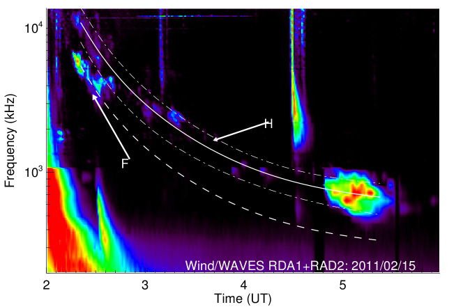
The radio emission associated with the CME-driven shock started at about 02:00UT, and was observed by two SWAVES instruments on board STEREO (Kaiser et al., 2008) and the WAVES instrument on board the WIND spacecraft (Bougeret et al., 1995). Figure 2 shows the strong intermittent type II burst in decameter to kilometer range recorded by WIND/Waves. From these recordings we distinguish two lanes which correspond to the fundamental plasma emission and its second harmonic.
3. Reconstructions
In this Section we describe the processing of the data and the shape and distance reconstruction of the CME based on it. A comparison of the individual results will follow in Section 4.
3.1. Reconstruction from stereoscopy
Coronagraph images only give the two-dimensional (2D) projection of CMEs onto the plane-of-sky (POS) normal to the respective view direction. Therefore, the speed obtained from the projected distance of the apparent CME leading edge is typically underestimated if the CME propagation direction is off the POS. For the halo CME investigated here, the propagation direction does not lie far from the POS of STEREO A and B. On the other hand, a genuine stereoscopic reconstruction is not straight forward, because STEREO A and B have almost opposite view directions, hence their image information is almost redundant while the view from SOHO does not allow to discern the leading edge. Instead it rather yields the lateral extent of the CME.
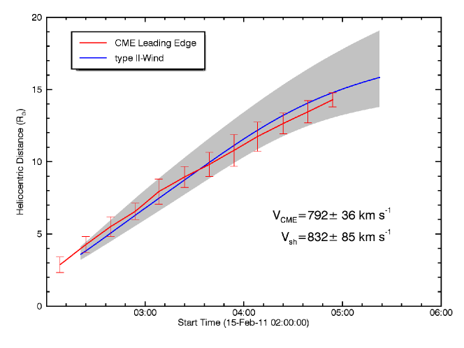
Using the data of STEREO/COR2 A and B, we measure the kinematics of the projected leading edge of the CME along different position angles (PAs) as indicated in Figure 1. The red line in Figure 3 shows the measured distance-time profile for the CME leading edge and the red vertical bars indicate the distance uncertainties which are due to the kinematic dependence on the PAs and the intensity drop off when identifying the outermost bright CME structure. The top and the bottom of the bars indicate the maximum and minimum heights of the CME leading edge from the Sun center along different PAs. The average propagation speed of the leading edge was estimated to be by linearly fitting the distance-time profiles along different PAs recorded by both STEREO/COR2 A and B.
As an alternative approach to stereoscopy, a fit of the visible CME boundaries in several coronagraph images with a parameterized flux rope CME model (GCSFM) has become popular (Thernisien et al., 2006,2009). While both methods rely on stereoscopy, the GCSFM fits the CME shape interactively to a family of flux-rope-like surfaces of six geometrical parameters, the line-tying approach does not make any a-priori assumptions about the CME shape but is often restricted to its leading-edge surface. We apply GCSFM to our data at the time when LASCO provided the polarized image set as shown in Figure 4, from which we estimate that at about 02:54 UT the CME propagated to a height of and its center was directed at a longitude of and latitude of in a carrington coordinate system. These values are also listed in Table 2.
3.2. Reconstruction from frequency inversion
The emission of Type II bursts is generally assumed to be produced by electron density fluctuations generated by energetic electron beams. The acceleration process is not known in detail, but there is strong evidence that it occurs in the vicinity of the shock which runs ahead of the CME front. If the CME front propagates within the solar wind frame at superalfvénic speed, the stand-off distance between CME front and the shock ahead should not change too much (Reiner et al., 1998). The instability of the electron beam generates electrostatic and by linear coupling also electromagnetic noise at the plasma frequency and its harmonics. The relation between the plasma frequency and the background electron density is (Priest, 1982):
| (1) |
The observation of the frequency with time can therefore be converted to a distance vs time estimate of the emission region from the Sun if an interplanetary plasma density model is assumed.
There is a variety of interplanetary density models, which were developed based on different measurements. Discrepancies become obvious when matching the IP densities with Active Region(AR) corona. For example, the model by Leblanc et al. (1998), which agrees well with in-situ observations by the Hellios spacecraft, gives too low densities when close to the Sun surface, especially when compared with the AR corona. On the other hand, the model by Saito et al. (1970), being very successful when applied to the AR corona, gives too high densities at large distances in IP space. In our analysis, we fit the visible parts of the type II burst to the model by Vršnak et al. (2004), who used the relation between the corona magnetic field and the height to smoothly connect the AR corona and IP space. The density model was normalized to the electron density at 1 AU of , the average value observed by Wind/SWE before CMEs arrived. The normalized density model is given by
| (2) |
where is the distance in unit of , .
To obtain smooth frequency drifts for the type II burst in the dynamic spectrum, we propose the following function according to the adopted density model,
| (3) |
where a,b,c,d are fit parameters which incorporate the still unknown speed and its possible time variation.
In Figure 2 we present our fitting results111Since the second harmonic lasts over a much longer time than the fundamental, we pick up a set of points from the radio spectrogram for the second harmonic branch and fitted them with the model given by Equation (3).. The dashed and solid lines represent the fundamental and its second harmonic plasma emission, respectively. For the the second harmonic emission we also fit the visible boundaries indicated by the dot-dashed lines. The difference between the dot-dashed lines will be used to estimate the relative position uncertainties of the radio source region. In our analysis, the second harmonic band was used to estimate the heliocentric distance of the source. The corresponding results are presented in Figure 3 (blue line). The gray region indicates the resulting uncertainty in the height of the radio source region. The average velocity of the radio source is estimated to be , which is slightly faster but still comparable to the speed determined form the leading edge of the CME seen in the STEREO images. The position of the radio source at 02:56:24 when SOHO/LASCO took the polarized image sequence is estimated to be between and .
3.3. Reconstruction from the Polarisation Ratio(PR) method
3.3.1 Method description
The polarization of sunlight scattered by corona electrons is well known (Billings, 1966). The scattering cross section depends on the angle between the scattering direction and the electric field vector. Since the light emitted from the photosphere is unpolarized, it can be split into two equal, mutually perpendicular components, one normal to and one in the scattering plane. From Thomson Scattering theory, the scattered intensity of the former (denoted as ) is independent of the scattering angle , while the scattered intensity of the latter (denoted as ) varies as . The polarized brightness , total brightness and polarization degree P are defined as
| (4) | |||||
| (5) | |||||
| (6) |
The expressions of and were given by, e.g., Howard & Tappin (2009):
| (7) | |||||
| (8) |
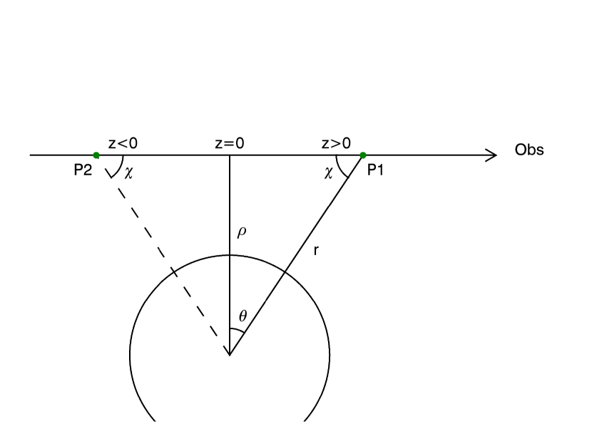
where is the intensity of solar disk center; is the Thomson scattering cross section; u is the limb-darkening coefficient; is the local electron density; is the projected distance along the POS; z is the distance along the line-of-sight from POS; and A, B, C, D could be expressed as functions of , the half-angle subtended by the solar disk at the scattering point,
| (9) | |||||
| (10) | |||||
| (11) | |||||
| (12) | |||||
where the angle is given by (r is the heliocentric distance in unit of solar radii , ). In Figure 5, we illustrate the geometry of these variables.
For each line of sight, a conventional assumption of the PR method is that all the electrons, which contribute to and , are located at one single position(, ) (indicated as P1 in Figure 5) which we refer to as the equivalent scattering center. The corresponding electron density is assumed to be , then Equations 7 and 8 can be converted to
| (13) | |||||
| (14) |
Under this assumption the polarization degree can be expressed as the ratio of polarized to the total brightness
| (15) |
where A,B,C,D and are functions of , .
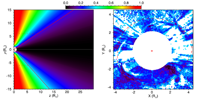
From Equation 15, the theoretically derived relationship between polarization degree P, projected distance and distance from POS for the equivalent scattering center is shown in the left panel of Figure 9. On the other hand, and can be obtained from observations and therefore it’s possible to get some estimate of the line-of-sight distance of the scatterers by solving (15) for .
However, the method has some drawbacks: The observed scattered signal is the result of a line-of-sight integration. Depending on the electron density distribution along the line-of-sight, the observed polarization degree is influenced from a wide distance range while the formal application of the relation in the left panel in Figure 9 just yields a single distance. Moreover, (15) depends on the square so that the sign of the distance of the equivalent scattering center from the plane-of-sky is ambiguous unless the context or measurements from another view point allow to distinguish whether the scatterer is in front or behind the plane-of-sky. For example, in Figure 5 points P1, P2 are equivalent and yield the same polarization ratio (Dai et al., 2014). On the day when the halo CME occurred, SOHO/LASCO C2 unfortunately produced only one polarized image sequence every six hours, and the CME was imaged in polarization mode only at a single instance at 02:56:54UT. We therefore have only one single polarized image set which we can use to compare the PR method with the distances estimated from the previous two methods.
In order to remove the background from the images and isolate the scattering of the CME alone, we need to subtract background images. Usually two kinds of methods for background subtraction are used. One method is to subtract the pre-event images which are taken just before the event, and the other method is to subtract minimum images build from the minimum value of each pixel over all the images during a specific time range (usually one month, which is long enough to subtract the F-corona and the stray light). In our case, the pre-event images were taken too early to remove the background well enough and a monthly minimum background leaves too many streamers so that the CME could not be well identified, therefore we produce a two-day minimum background from the polarized images taken on 14-15 February 2011 for each of the three polarizers at , , . We subtracted the respective background from the three primary polarized brightness images rather than to subtract a background from the archived pB image. because the polarized brightness is non-linearly related to the primary measurements, It therefore makes a difference to the conventional approach to subtract the background from the archived ready-made pB images. Naming the polarized brightness at polarization angle with the respective background subtracted, the polarized brightness , total brightness and polarization degree of the CME are determined from(Billings, 1966)
| (16) | |||||
| (17) | |||||
| (18) |
Before calculating the polarization degree, we run a 3-by-3-pixel averaging box over the synthesized pB and tB images to increase the signal-to-noise ratio and reduce the possible error caused by the CME motion during the exposures of the three polarizers. In Figure 6 we show our analyses of the LASCO polarimetric observations for the large-scale quiet Sun in upper panels and for the investigated CME in lower panels. The quiet Sun polarimetric observations were taken at 02:56:30 on 14 February 2011 when no CMEs appeared in the field of view(FOV) of C2. A monthly minimum background was subtracted from each polarized image before synthesizing tB and pB. Quite a number of streamer structures can be clearly distinguished in the latitude range from about -60 to 60 degrees. Our analyses indicate that streamers have relatively larger polarization degree and smaller distances from POS than the ambient corona, which are consistent with the theoretical predictions. The lower panels display the polarimetric observations of the halo CME taken at 02:56:24 on 15 February 2011. Unlike the quiet Sun, a two-day minimum background was subtracted from each polarized image to show the CME structure as clearly as possible. Details of the structures appearing in the polarimetric images will be presented in the following Section.
3.3.2 Different features in C2 images
The image of the polarization degree of the halo CME in Figure 6 shows a wealth of coronal structures which were superposed by the line-of-sight integration. The color code represents the polarization ratio and helps to separate features from different depths. We can distinguish bright background streamer structures which have not been eliminated by the two-day minimum background subtraction. To single out the halo CME in the foreground, we try to identify and discard the near-Sun coronal background based on the polarization ratio. We have marked some of the presumable background features with enhanced polarization (marked by F1, F2, F3)in Figure 6.
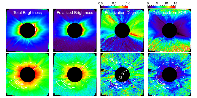
F1 has a high polarization and extends radially from the occulter edge to 2.6 . The polarization and shape suggest that the feature can be attributed to a streamer in the background corona, not far from the POS.
F2 also has a relatively high polarization but is oriented azimuthally. It is well embedded inside the projection of the halo CME. Because of its shape we have to rule out a streamer but our suspicion is that it is due to the leading edge of a fairly weak and slow CME (CME1) which was launched about one hour before the fast and strong halo CME studied here (CME2). In Figure 7 we show the propagation of both CMEs. CME1 first appeared in the field of view of STEREO/COR2 at 00:54UT. Its propagation speed was estimated to be along a direction with longitude of and latitude of in Carrington coordinates using the triangulation of the leading edges observed by STEREO/COR2/A and LASCO/C2 respectively. CME1 was eventually submerged by CME2 in the both images of STEREO/COR2/A and LASCO/C2 . It is not clear how much the two CMEs interacted, but in Figure 2 a radio emission enhancement around 02:40UT between the fundamental and its second harmonic could be related to such an interaction of the two CMEs(Gopalswamy, 2004).
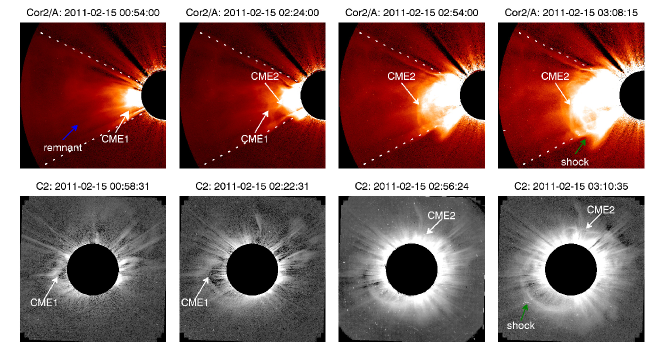
In the period 13-15 February 2011, a series of CMEs were launched successively from the active region AR 11158 (Maričić et al., 2014). A number of them occurred even before CME1 in this time period. One of them launched at 17:20 UT on 2011 February 14 also interacted with the halo CME studied here. This interaction occurred at about 06:49 UT on 2011 February 15 and has been studied in detail by Temmer et al. (2014). From the images of STEREO/COR2 (upper panels in Figure 7), we can distinguish some remnant from these preceding CMEs which are widely distributed within a cone. Their brightness is slightly enhanced in the region between two dotted lines in Figure 7. Besides the remnant, we can also distinguish a fairly weak CME-driven shock, indicated by the green arrows in Figure 7. The shock was visible at 03:10 UT in the next frame after 02:56 UT when the polarimetric observations of the CME were taken. At 02:56 UT, it is very difficult to identify the shock structure. Therefore, we suspect that both the remnant and the possible CME-driven shock may contribute to F3. However, considering the weakness of the shock, probably F3 mainly comes from the remnant.
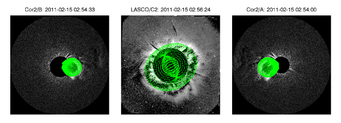
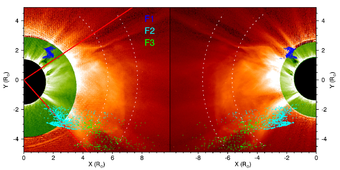
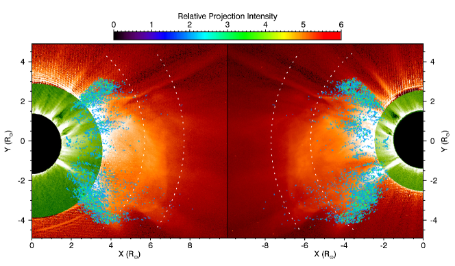
The various features derived from LASCO C2 should match corresponding white-light structures seen from STEREO. In Figure 8 the 3D position of the scattering centers of different features were projected onto the white-light total brightness images observed at the same time by STEREO A and B. As the view direction of LASCO on 15 Feb 2011 is almost at right angles with the STEREO spacecraft, the -coordinate of the equivalent scattering centers is almost entirely given by their depth from the PR method. As a reference, the dotted curves represent the uncertainty for the radial distance of the radio source region estimated from the radio observations, as discussed in Section 3.2.
3.3.3 Separation of CME and background in image of polarization degree
In order to improve the reliability of 3D reconstruction of the halo CME investigated here with the PR method, we attempt to separate the CME features from the background structures discussed in Section 3.3.2. According to Thomson Scattering theory, the farther away of the electrons from POS, the lower the polarization degree of scattered light. The left panel of Figure 9 shows the theoretical relationship between P (polarization degree), z (distance from the POS) and (distance along the POS). From the limb views, most CMEs can be seen to propagate within a limited angular cone with a half width often of less 45 degrees. The boundary of the cone should give an upper limit of the observed polarization degree. It is found that the contour lines of constant polarization degree beyond a distance of 1 to 2 are cone-shaped as well. Therefore, we conclude that the plasma cloud of a well centered halo CME (it would propagate outwards along the z direction in the left panel of Figure 9 ) should produce coronagraph polarization ratios below about 0.4 once it has propagated more than 1 to 2 from the POS. If this CME propagates self-similarly, the maximum polarization degree would not change much.
For our CME, after varying the threshold of polarization degree in a certain range, we found 0.4 is a good value for separating the CME. Such a selection is further verified by the cone distinguished from the white-light images of STEREO/COR2 shown in the left panel of Figure 8 by two red solid lines. The CME cone is over-plotted by the red solid lines in the left panel of Figure 9. The FOV of LASCO/C2 is marked by red parallel dotted lines(the inner boundaries at are caused by the LASCO/C2 occulter). It is obviously that the CME cone locates within a contour level of 0.4. We therefore use a polarization degree of 0.4 as a criterion to separate CME signals from the background. We show our separating result in the right panel of Figure 9. The image has been enlarged so as to see the details of the cleaned CME. The red dashed curve indicates the boundary of the CME identified from white-light observations by LASCO/C2. We will use this cleaned image to estimate the 3D structure of the CME.
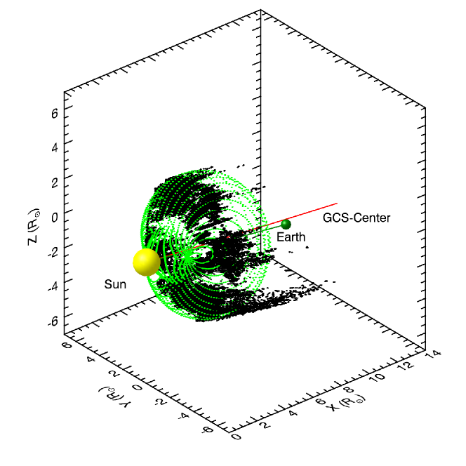
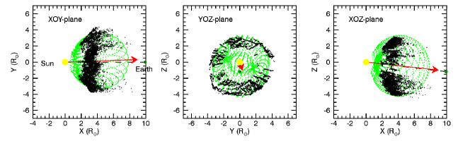
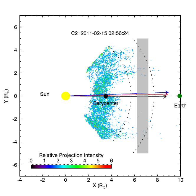
Similar to the projection of the three background features, Figure 10 shows the projection of the reconstructed CME with background structures removed. The color bar displays the relative projection intensity222We calculate the relative projection intensity by summing the number of projected 3D CME points in each pixel along the projection direction.The lack of points at the CME front is due to the occultation of the CME front in the LASCO view, which is an unavoidable problem for coronagraph observations of halo CMEs. To give an impression of the entire CME we combine the PR method with the GCSFM (GCS-PR) fit procedure applied only to the LASCO observations. We first apply the GCSFM to the LASCO C2 total brightness image to get a first estimate of the free parameters, and then use the 3D points derived from polarimetric method to further constrain the GCSFM parameters. Hence the GCSFM results is only based on LASCO halo CME observations. Figure 11 shows the fitting result of this method, from which we estimate that the CME has reached a height of with a direction of longitude and latitude in the carrington coordinate system at the time when the LASCO polarization images were observed. This height lies at the upper limit of the height range determined from the radio frequency measurement and the leading edge observed from STEREO (see Figure 3).
4. Comparison
Figure 3 summarizes the propagation of the projected CME leading edge triangulated from the stereo observations and the path of the radio source derived from the frequency drift and the interplanetary density model by Vršnak et al. (2004). The uncertainty of the radio source position is indicated by the gray region, and the uncertainties of the leading edge are indicated by the vertical bars. The radio source propagation of the type II burst are found to be very close to the leading edge of the CME, which complies well with the scenario of a CME-driven shock wave. The region of radio emission seems to spread out with distance and appears to move slightly faster than the leading edge of the CME.
Due to the viewing geometry, the positions of the equivalent scattering centers calculated by the PR method and overplotted into STEREO white-light images should match respective white-light features in these images. The scattering center, however, at best represents a mean depth position which may agree with the real electron density distribution only if it is concentrated in depth. Therefore we found it therefore necessary to separate features of different depth in the polarization degree images and compare them individually. In Figure 8 we present the projection of three features onto the white-light images of STEREO/A and B. The projection of the separated CME is shown in Figure 10. We find that the equivalent scattering centers are consistent with the observations from STEREO, which confirms that the PR method yields reasonable results.
The line-of-sight integration effect is even more pronounced for the halo CME. The CME is a distributed density cloud, and we cannot expect that the distribution of the scattering centers we attributed to the CME exhibit its entire shape. For a quantitative comparison, we combine these scattering centers to their barycenter and compare it to the GCSFM fitting results and to the location of the leading edge derived from STEREO observations. This comparison is shown in Figure 12. The grey region indicates the distance range of the CME leading edge from the STEREO observations and the two dotted lines represent the possible boundaries of the radio source region at the time when the polarized images were taken by LASCO. The barycenter of the equivalent scattering centers was found at a distance of from the Sun center, about behind the leading edge at the time when the LASCO polarized images were taken. This discrepancy is for once due to the line-of-sight integration effect which causes the scattering centers to represent the entire CME density rather than the leading edge. In addition, the occultation of the central CME region from the LASCO observations may also play a role. In Figure 10, where we have overplotted the equivalent scattering centers attributed to the CME on top of the STEREO images it is obvious that some central and most advanced parts of the CME cloud are not covered by equivalent scattering centers.
The directions of the CME estimated from both GCSFM to image triplets (GCS-Tri) and GCSPFM to PR results(GCS-PR) are very close to the CME barycenter direction. A comparison between GCS-Tri and GCS-PR is shown in Table 2. The difference seems very small, which indicates that a combination of GCSFM with PR method could be a feasible approach to measure the propagation direction and distance of a halo CME from a single perspective at Earth.
| GCS-PR | GCS-Tri | |
|---|---|---|
| Longitude(∘) | 23.14 | 22.14 |
| Latitude(∘) | -6.30 | -9.30 |
| Height() | 7.90 | 7.10 |
5. Summary
The goal of this study was to explore the possibilities to measure the approach of a halo CME to Earth by observations from the Earth-direction alone. In the not too far future, when STEREO will not be available any more, these observations will be the only data on which a CME warning could be built upon. We focused in particular two methods to achieve this goal: type II radio burst inversion and polarization ratio method. For this study, we select a full halo CME on 15 February. On that day, STEREO A and B each had a separation angle of about with SOHO, which means the halo CME moved close to the POS with respect to STEREO A and B. Firstly, this allowed to directly and reliably record the propagation of the CME leading edge as a reference for the results of the other two methods. Secondly, the favorable viewing geometry of the three spacecraft allowed to compare the depth estimates derived from polarized images taken by LASCO directly with corresponding white-light features in the STEREO image set.
Unfortunately, LASCO only produced a single polarimetric image set of the halo CME at about 02:54 so that we could compare the results of the PR method only for this single instance. Coronagraph images of a halo CME are heavily contaminated by different background structures as seen, for example, in Figure 6. Using images of the polarization ratio can greatly help to disentangle the various structures and separate the CME signals from the background. In our case, we combine the CME cone observed by STEREO/COR2 with the theoretical model of polarization degree to obtain a criterion value(polarization degree = 0.4) for separating the CME signals. The result of this separation was demonstrated in the right panel of Figure 9. In future, for the case of lacking STEREO observations, we maybe apply the typical cone model to get an estimate of the criterion of polarization degree(Zhao et al., 2002; Xie et al., 2004).
The comparison of the depth estimates from the PR method with white-light features in the STEREO images shows good consistency if the comparison is made for individual features identified in the polarization ratio images by a locally uniform polarization ratio. The more diffuse CME cloud, on the other hand has a large depth extent while the PR method yields only a single representative depth estimate for each pixel analyzed. A relationship of the position of the equivalent scattering centers with the CME leading edge is not easily established. The maximum distance of the scattering centers from the Sun is a statistically very noisy measure. The barycenter of the equivalent scatterers, even when cleaned from background features, gave a distance of about half of the leading edge distance. Further studies like the one presented here might eventually yield a well defined correction factor between the barycenter and the leading edge distance. We found it helpful to combine the PR method with the GCSFM fit to derive the probable shape of the CME cloud which gave a better match for the leading edge distance estimate and also for the direction of the CME propagation.
The second method to analyze the time-frequency variation of the type II radio burst associated with the CME also has some uncertainties. The most critical assumption is the interplanetary density model required to convert plasma frequency into distance from Sun center. We found the model developed by Vršnak et al. (2004) gave the best agreement to the kinematics of the leading edge as derived from the STEREO observations. This comparison is summarized in Figure 3. The discrepancy in the estimated velocities amounted to about 5% with the radio burst frequency giving a slightly faster speed estimate. Extensions of the method used here also analyze the correlation of the radio burst signal in different antenna polarizations from which the direction and the size of the radio source can be estimated (Manning & Fainberg, 1980; Cecconi & Zarka, 2005).
A problem with the radio frequency method for routine CME arrival predictions is that not all CMEs emit a well identifiable signal. For that reason, the PR method, even though it yields less precise results should be considered as a back-up when the radio signals are too weak or are missing completely. We hope that an extension of the study presented in this paper to more halo CME events will help to improve the analysis of the PR method and eventually lead to more precise CME predictions.
Acknowledgments
We acknowledge the use of data from STEREO, SOHO and WIND. Many thanks to Thomas G. Moran and Angelos Vourlidas for their helpful discussions on dealing with LASCO polarimetric data. This work was supported by the NSFC grants (11522328, 11473070, 11427803, 11233008 and 11273065) and by the Strategic Priority Research Program, the Emergence of Cosmological Structures, of the Chinese Academy of Sciences, Grant No. XDB09000000. L.F. also acknowledges the Youth Innovation Promotion Association and the specialized research fund from State Key Laboratory of Space Weather for financial support.
References
- Aschwanden et al. (2008) Aschwanden, M. J., Burlaga, L. F., Kaiser, M. L., et al. 2008, Space Sci. Rev., 136, 565
- Bale et al. (1999) Bale, S. D., Reiner, M. J., Bougeret, J.-L., et al. 1999, Geophys. Res. Lett., 26, 1573
- Billings (1966) Billings, D. E. 1966, A guide to the solar corona
- Bougeret et al. (1995) Bougeret, J.-L., Kaiser, M. L., Kellogg, P. J., et al. 1995, Space Sci. Rev., 71, 231
- Brueckner et al. (1995) Brueckner, G. E., Howard, R. A., Koomen, M. J., et al. 1995, Sol. Phys., 162, 357
- Cecconi & Zarka (2005) Cecconi, B., & Zarka, P. 2005, Radio Science, 40, RS3003
- Dai et al. (2014) Dai, X., Wang, H., Huang, X., Du, Z., & He, H. 2014, ApJ, 780, 141
- Dere et al. (2005) Dere, K. P., Wang, D., & Howard, R. 2005, ApJ, 620, L119
- Domingo et al. (1995) Domingo, V., Fleck, B., & Poland, A. I. 1995, Sol. Phys., 162, 1
- Facius & Reitz (2006) Facius, R., & Reitz, G. 2006, in European Planetary Science Congress 2006, 267
- Feng et al. (2013) Feng, L., Inhester, B., & Mierla, M. 2013, Sol. Phys., 282, 221
- Feng et al. (2012) Feng, L., Inhester, B., Wei, Y., et al. 2012, ApJ, 751, 18
- Gan et al. (2015) Gan, W., Deng, Y., Li, H., et al. 2015, in Proc. SPIE, Vol. 9604, Solar Physics and Space Weather Instrumentation VI, 96040T
- Gopalswamy (2004) Gopalswamy, N. 2004, Planetary and Space Science, 52, 1399
- Howard & Tappin (2009) Howard, T. A., & Tappin, S. J. 2009, Space Sci. Rev., 147, 31
- Inhester (2006) Inhester, B. 2006, ArXiv Astrophysics e-prints, astro-ph/0612649
- Inhester (2015) —. 2015, ArXiv e-prints, arXiv:1512.00651
- Kaiser et al. (2008) Kaiser, M. L., Kucera, T. A., Davila, J. M., et al. 2008, Space Sci. Rev., 136, 5
- Leblanc et al. (1998) Leblanc, Y., Dulk, G. A., & Bougeret, J.-L. 1998, Sol. Phys., 183, 165
- Magdalenić et al. (2014) Magdalenić, J., Marqué, C., Krupar, V., et al. 2014, ApJ, 791, 115
- Manning & Fainberg (1980) Manning, R., & Fainberg, J. 1980, Space Science Instrumentation, 5, 161
- Maričić et al. (2014) Maričić, D., Vršnak, B., Dumbović, M., et al. 2014, Sol. Phys., 289, 351
- Martínez Oliveros et al. (2012) Martínez Oliveros, J. C., Raftery, C. L., Bain, H. M., et al. 2012, ApJ, 748, 66
- Mierla et al. (2009) Mierla, M., Inhester, B., Marqué, C., et al. 2009, Sol. Phys., 259, 123
- Mierla et al. (2010) Mierla, M., Inhester, B., Antunes, A., et al. 2010, Annales Geophysicae, 28, 203
- Moran & Davila (2004) Moran, T. G., & Davila, J. M. 2004, Science, 305, 66
- Moran et al. (2010) Moran, T. G., Davila, J. M., & Thompson, W. T. 2010, ApJ, 712, 453
- Nandi (2015) Nandi, D. 2015, IAU General Assembly, 22, 2253490
- Pirjola (2002) Pirjola, R. 2002, in ESA Special Publication, Vol. 477, Solspa 2001, Proceedings of the Second Solar Cycle and Space Weather Euroconference, ed. H. Sawaya-Lacoste, 497–503
- Priest (1982) Priest, E. R. 1982, Geophysics and Astrophysics Monographs, 21
- Reiner et al. (1998) Reiner, M. J., Kaiser, M. L., Fainberg, J., Bougeret, J.-L., & Stone, R. G. 1998, Geophys. Res. Lett., 25, 2493
- Saito et al. (1970) Saito, K., Makita, M., Nishi, K., & Hata, S. 1970, Annals of the Tokyo Astronomical Observatory, 12, 53
- Shen et al. (2013) Shen, C., Liao, C., Wang, Y., Ye, P., & Wang, S. 2013, Sol. Phys., 282, 543
- Su et al. (2016) Su, W., Cheng, X., Ding, M. D., et al. 2016, ApJ, 830, 70
- Temmer et al. (2014) Temmer, M., Veronig, A. M., Peinhart, V., & Vršnak, B. 2014, ApJ, 785, 85
- Thernisien (2011) Thernisien, A. 2011, ApJS, 194, 33
- Thernisien et al. (2009) Thernisien, A., Vourlidas, A., & Howard, R. A. 2009, Sol. Phys., 256, 111
- Thernisien et al. (2006) Thernisien, A. F. R., Howard, R. A., & Vourlidas, A. 2006, ApJ, 652, 763
- Velli (2013) Velli, M. M. 2013, AGU Spring Meeting Abstracts
- Vršnak et al. (2004) Vršnak, B., Magdalenić, J., & Zlobec, P. 2004, A&A, 413, 753
- Xie et al. (2004) Xie, H., Ofman, L., & Lawrence, G. 2004, Journal of Geophysical Research (Space Physics), 109, A03109
- Zhao et al. (2002) Zhao, X. P., Plunkett, S. P., & Liu, W. 2002, Journal of Geophysical Research (Space Physics), 107, 1223
- Zhukov (2014) Zhukov, A. 2014, in COSPAR Meeting, Vol. 40, 40th COSPAR Scientific Assembly