High-$\beta$ equilibrium and ballooning stability of the low aspect ratio CNT stellarator

Abstract

The existence and ballooning-stability of low aspect ratio stellarator equilibria is predicted for the Columbia Neutral Torus (CNT) with the aid of 3D numerical tools. In addition to having a low aspect ratio, CNT is characterized by a low magnetic field and small plasma volume. Also, highly overdense plasmas were recently heated in CNT by means of microwaves. These characteristics suggest that CNT might attain relatively high values of plasma beta and thus be of use in the experimental study of stellarator stability to high-beta instabilities such as ballooning modes. As a first step in that direction, here the ballooning stability limit is found numerically. Depending on the particular magnetic configuration we expect volume-averaged $\beta$ limits in the range 0.9-3.0%, and possibly higher, and observe indications of a second region of ballooning stability. As the aspect ratio is reduced, stability is found to increase in some configurations and decrease in others. Energy-balance estimates using stellarator scaling laws indicate that the lower $\beta$ limit may be attainable with overdense heating at powers of of 40 to 100 kW. The present study serves the additional purpose of testing VMEC and other stellarator codes at high values of $\beta$ and at low aspect ratios. For this reason, the study was carried out both for free boundary, for maximum fidelity to experiment, as well as with a fixed boundary, as a numerical test.

I Introduction

To date, the highest plasma beta among stellarators—about 5%—have been obtained in W7-AS Weller et al. (2003) and in LHD Sakakibara et al. (2015). Neither plasma was found to be unstable, implying even higher stability limits in those devices. Therefore, to date analytical and numerical investigations of ballooning modes Cuthbert et al. (1998); Hegna and Nakajima (1998); Hudson and Hegna (2003, 2004); Rafiq et al. (2010) and other high-$\beta$ instabilities Nielson et al. (2000) have only received partial validation by experiment: experiments confirmed certain values of $\beta$ to be stable, but could not verify whether even higher values were unstableWeller et al. (2001, 2003). Experimental access to the stellarator $\beta$ limit and experimental characterization of instabilities would finally enable comparison with theory and improve our understanding and predictive capability. Access to higher $\beta$ (and, yet, stability) could also lead to more compact and efficient stellarator reactor designs, currently assuming volume-averaged beta $\langle\beta\rangle=$ 3-6% Beidler et al. (2001); Sagara, Igitkhanov, and Najmabadi (2010). In fact, the main optimization criterion in the HELIAS reactor is to maintain a stability limit $\langle\beta\rangle>4\%$ while reducing the Pfirsch-Schlüter currents and Shafranov shift Beidler et al. (2001).

In the present work, it is argued that the Columbia Neutral Torus (CNT) stellarator at Columbia University (Fig. 1) is uniquely well-suited for this research. The device, originally constructed to study non-neutral and pure-electron plasmas Pedersen et al. (2004, 2006); Kremer et al. (2006); Sarasola and Pedersen (2012), has since been repurposed to investigate quasi-neutral plasmas, and has addressed issues relevant to magnetic fusion energy such as error-field diagnosis Hammond et al. (2016a) and processing of stellarator images Hammond et al. (2016b). From the point of view of high $\beta$ stability, CNT is attractive for two main reasons: (1) it could reach high values of $\beta$ by deploying relatively small amounts of heating power and (2) its stability limit is expected to be lower and thus more easily accessible than in other devices.

Regarding the first point, the CNT magnetic field is low: in general $B<0.3$ T, but $B<0.1$ T was adopted for this work. As a result, the magnetic pressure $B^{2}/2\mu_{0}$ is very low, and more amenable plasma pressures (2500 times lower than in a 5 T reactor, if not smaller) suffice to reach high $\beta$. The need for high plasma pressure will require heating at high density. In this regard, overdense plasma heating, at densities in excess of four times the cutoff density, was recently observed in CNT by injecting 10 kW microwaves at 2.45 GHz. Increasing the heating power would result in high power densities in the small CNT plasma ($V\approx 0.1\text{m}^{3}$). On the other hand, the small size of CNT is co-responsible for poor energy confinement. Even so, scaling-law calculations to be presented in this paper suggest that hundreds of kW of microwave power might be sufficient for high $\beta$.

Regarding the second point, CNT is a classical, non-optimized stellarator. In particular, it was not optimized for high stability, making its stability limit lower and easier to access. An interesting competing effect might arise from the CNT low aspect ratio, $A\geq 1.9$. This characteristic, relatively under-explored in stellarators, increased the stability limit in spherical tokamaks and favored the achievement of higher $\beta$ compared to tokamaks . It is interesting to verify whether the low aspect ratio has a similar beneficial effect on stellarator stability, although evidence presented below suggests this not to be the case, at least not for CNT.

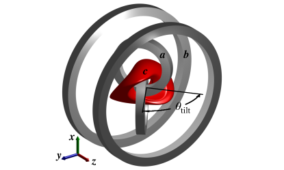
Figure 1: Schematic of the CNT coil configuration. (a) interlocked (IL) coils; (b) poloidal field (PF) coils; (c) last closed flux surface. Adapted with permission from Ref. Hammond et al. (2016a).

This paper describes a numerical investigation of high-$\beta$ equilibria that are attainable in the CNT configuration. Equilibria are calculated using the VMEC code,Hirshman and Whitson (1983) which solves the ideal MHD equations for input vacuum fields and profile functions. They are then evaluated for stability using COBRAVMEC,Sanchez et al. (2000) which determines ballooning growth rates at various locations in the plasma. The structure is as follows: Sec. II briefly overviews considerations for calculating VMEC equilibria in the CNT configuration and presents some fixed-boundary results. Sec. III reviews the assumptions used for calculations of equilibrium parameters, bootstrap current, and stability. The methods for the calculations are then described in Sec. IV. Sec. V presents the main free-boundary equilibrium and stability results. Sec. VI describes scaling-law calculations to predict how much heating power will be necessary to attain the equilibria in Sec. V.

II Fixed-boundary VMEC solutions for CNT geometry

VMEC may assume a fixed or free plasma boundary depending on the purpose of the calculation. In fixed-boundary mode, the plasma boundary is assumed to be known ab initio and the full magnetic field is determined in the calculation without knowledge of the external coils. In free-boundary mode, the coil configuration and the field that it generates are known and the plasma boundary is determined using an energy principle.Hirshman, van Rij, and Merkel (1986) Free-boundary mode was used in this work because the shape of the plasma boundary was expected to vary with $\beta$ and plasma current.

As an initial test of concept, however, a number of high-$\beta$ calculations were performed in fixed-boundary mode for CNT-like configurations. One example is shown in Fig. 2. In this case, the boundary was set to conform to the last closed flux surface (LCFS) obtained from vacuum field line calculations with $\theta_{\text{tilt}}=78^{\circ}$ and $I_{IL}/I_{PF}=2.5$. Here $\theta_{\text{tilt}}$ denotes the tilt angle between the interlocked (IL) coils (Fig. 1). This angle can be set to $64^{\circ}$, $78^{\circ}$, or $88^{\circ}$. $I_{IL}/I_{PF}$ is the ratio of currents flowing in the IL and poloidal field (PF) coils. For this choice of $\theta_{\text{tilt}}$ and $I_{IL}/I_{PF}$, fixed-boundary equilibria were obtainable for $\langle\beta\rangle$ up to $6.6\%$ (Fig. 2). The relative Shafranov shift $\Delta R/a_{h}$, defined according to Ref. Weller et al. (2006) as the horizontal shift $\Delta R$ in the magnetic axis over the horizontal minor radius $a_{h}$, is seen to increase linearly with $\beta$, as expected (Fig. 2b). While these results are not particularly relevant to future comparisons with experiment, they are useful nonetheless as a verification that VMEC yields reasonable results at high beta and low aspect ratio, comparable to calculations made for a spherical stellarator concept in Ref. Moroz (1996).

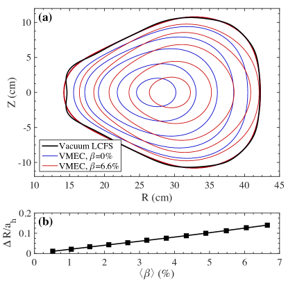
Figure 2: Results of a series of fixed-boundary simulations of CNT with $\theta_{\text{tilt}}=78^{\circ}$, $I_{IL}/I_{PF}=2.5$, $I_{\text{p}}=0$, and a centrally peaked pressure profile as shown in Fig. 3. (a) Flux surface comparison between calculations with $\langle\beta\rangle=0\%$ and $\langle\beta\rangle=6.6\%$, with the vacuum last closed flux surface (LCFS) as a reference; (b) Relative Shafranov shift as defined in the text.

III Input parameters

CNT’s field strength for electron cyclotron heated (ECH) plasmas, and possibly electron Bernstein wave heated (EBWH) plasmas, is constrained by the requirement for $|\mathbf{B}|=0.0875$ T for heating at the first electron cyclotron harmonic or $|\mathbf{B}|=0.0437$ T for the second harmonic at 2.45 GHz. With $|\mathbf{B}|$ fixed, the only two degrees of freedom controlling the vacuum-field configuration are $\theta_{\text{tilt}}$ and $I_{IL}/I_{PF}$.

The size of the free boundary is determined by the total enclosed magnetic flux. This was chosen to approximately equal the flux enclosed in the vacuum-field LCFS for the respective configuration.

Pressure profiles were assumed to have one of the two functional forms shown in Fig. 3. The hollow profile corresponds to a typical Langmuir probe measurements of ECH plasmas in CNT. The peaked profile shown was also considered for comparison, because peaked profiles cannot be ruled out from future experiments.

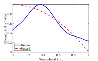
Figure 3: Normalized profiles of pressure used as inputs for the calculations in this paper. During the $\beta$ scans, each of these profiles was scaled according to the desired $\beta$ value.

As CNT does not have a solenoid transformer and does not deploy any form of current drive (EC, EBW, or other), the toroidal current density was assumed to be equal to the bootstrap current density, $J_{\text{bs}}$. Profiles of $J_{\text{bs}}$ were calculated for each equilibrium using the BOOTSJ code, which evaluates bootstrap currents in nonaxisymmetric plasma configurations using the drift kinetic equation.Shaing et al. (1989)

Since BOOTSJ requires the electron density and the electron and ion temperatures as inputs, these quantities were estimated as follows. For equilibria with the hollow (experimentally obtained) pressure profiles, the electron temperature profile was chosen to resemble the corresponding temperature measurements. For equilibria with the peaked pressure profiles, since no corresponding experimental data are available, temperature profiles were assumed to be flat. As CNT does not employ any direct ion heating mechanisms, the ion temperature was assumed to be 0.3 times the electron temperature at all locations. The electron temperature was constrained to not exceed 30 eV (hence, increases in $\beta$ were mostly driven by increases in density). The desire for low temperature and high density arises from the energy confinement scaling (Eq. 2). We impose a lower limit of 30 eV to avoid excessive radiative losses associated with peak radiation from hydrogen isotopes, other working gases such as noble gases, and common impurities such as oxygen and carbon.Post et al. (1977)

IV Methods for equilibrium and stability calculations

The maximum achievable $\beta$ for each configuration (defined by $\theta_{\text{tilt}}$, $I_{IL}/I_{PF}$, field strength, and pressure profile) was determined using the following procedure:

1. Conduct a free-boundary VMEC calculation with $\beta=0$ and zero toroidal current.

2. Using the results of the previous step as an initial guess, determine a free-boundary equilibrium with the pressure incrementally increased in magnitude (while maintaining the profile shape in Fig. 3).

3. Calculate the bootstrap current profile, $dI_{\text{bs}}/d\psi_{n}$, from the result of the previous step. $\psi_{n}$ is the normalized toroidal magnetic flux, which is used as a surface coordinate.

4. Re-calculate the equilibrium in step 2, incorporating the output from step 3 to obtain a self-consistent result.

5. Repeat steps 2-4 until either: (1) VMEC fails to descend robustly to an equilibrium solution or (2) the solution is not stable to ballooning instabilities, as determined below.

Each self-consistent equilibrium was evaluated for ballooning stability by the COBRAVMEC code, which computed growth rates on a grid of 1620 locations (15 toroidal $\times$ 18 poloidal $\times$ 6 radial) throughout the plasma volume. The maximum among these values was defined as $\gamma_{\text{max}}$. $\gamma_{\text{max}}$ was recorded for each equilibrium (i.e., for each $\beta$ increment) such that $\gamma_{\text{max}}$ could be plotted as a function of $\beta$. The maximum ballooning-stable $\beta$ was then defined as the highest value of $\langle\beta\rangle$ for which $\gamma_{\text{max}}<0$. This was obtained through interpolation of $\gamma_{\text{max}}(\beta)$ (as in, for example, Fig. 5c).

This procedure was carried out in three different plasma parameter regimes. The first used the experimental hollow pressure profile (Fig. 3) and a magnetic field strength $|\mathbf{B}|$ appropriate for first-harmonic ECH (denoted hereafter by $B\approx 0.08$ T). The second used the same pressure profile but half the field strength as is appropriate for second-harmonic ECH (denoted by $B\approx 0.04$ T). The third used the peaked pressure profile and $B\approx 0.08$ T.

V Free-boundary and stability results

Maximum volume-averaged $\beta$ values for attainable tilt angles and current ratios are plotted in Fig. 4 alongside other quantities of interest. The highest volume-averaged $\beta$ not vulnerable to ballooning instability was 3.0%. This was obtained in two configurations, one with $B\approx 0.04$ T and $I_{IL}/I_{PF}=2.75$; the other with $B\approx 0.08$ T and $I_{IL}/I_{PF}=3.25$. Both had $\theta_{\text{tilt}}=78^{\circ}$ and the hollow pressure profile. The latter is expected to be easier to attain experimentally due to the favorable scaling of confinement time with $B$ (Eq. 2) and will be referred to hereafter as the high-$\beta$ configuration. The highest stable $\beta$ values attained in the other two tilt angles were 2.5% for $\theta_{\text{tilt}}=88^{\circ}$ and 1.8% for $\theta_{\text{tilt}}=64^{\circ}$. Open markers in Fig. 4 represent configurations in which the VMEC code did not find equilibria that were ballooning-unstable. In other words, the actual $\beta$ limit for the configurations denoted by open symbols could be even higher than shown in Fig. 4. One such configuration is the high-$\beta$ configuration described above: its $\beta$ limit could in fact be higher than 3%.

The lowest $\beta$ threshold for ballooning stability (0.9%) was found in a configuration with $\theta_{\text{tilt}}=88^{\circ}$ and the peaked pressure profile. This will be referred to hereafter as the least stable configuration. The evolution of some key parameters for this and the high-$\beta$ configuration during the $\beta$ scan are shown in Fig. 5. The nonlinearity in relative Shafranov shift $\Delta R/a_{h}$ (Fig. 5b) is due to the change in the shape of the plasma with $\beta$, resulting in a non-constant $a_{h}$.

Note that while the least stable configuration initially becomes unstable at $\beta=0.9\%$, it exhibits a second region of stability for $1.1\%<\beta<1.5\%$ (Fig. 5c), probably due to the high bootstrap current (Fig. 5a) and consequently high shear. Second regions of ballooning stability have been the subject of theoretical research for both tokamak and stellarator configurations (for example, Refs. Greene and Chance (1981); Hudson and Hegna (2003, 2004)). Fig. 6 shows that this region could be accessed by a proper “trajectory” in a two-dimensional space spanned by heating power (roughly proportional to $\beta$ and to the pressure gradient) and coil-current ratio (controlling the $\iota$ profile, hence magnetic shear).

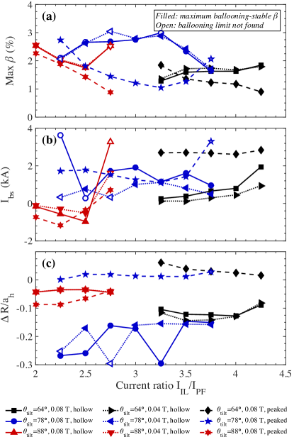
Figure 4: (a) Highest volume-averaged $\beta$, (b) bootstrap current, and (c) relative Shafranov shift as functions of the coil current ratio ($I_{IL}/I_{PF}$) and $\theta_{\text{tilt}}$ for the three different configurations of pressure and field strength discussed in the text. Here, “highest $\beta$” refers to the highest value before the plasma becomes ballooning-unstable (filled symbols) or the highest value for which it was possible to compute a stable equilibrium, without however encountering the ballooning stability limit yet (open symbols; see also Fig. 5c). Some markers overlap one another due to similar results.

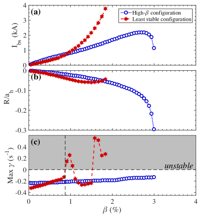
Figure 5: Evolution of key paramaters during the $\beta$ scan carried out for the high-$\beta$ magnetic configuration ($\theta_{\text{tilt}}=78^{\circ}$, $I_{IL}/I_{PF}=2.75$, $B=0.04$ T, hollow pressure profile) and for the configuration that became ballooning-unstable at the lowest $\beta$ ($\theta_{\text{tilt}}=88^{\circ}$, $I_{IL}/I_{PF}=2.75$, $B=0.08$ T, peaked pressure profile). The vertical dashed line indicates the value of $\beta$ at which the least stable configuration first becomes ballooning unstable. (a) bootstrap current; (b) relative Shafranov shift; (c) maximum calculated ballooning growth rate within the plasma volume. Note that the growth rate never becomes positive for the high-$\beta$ configuration.

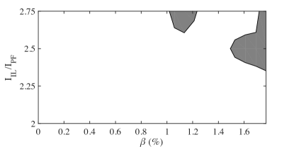
Figure 6: Contour plot of ballooning stability in $(\beta,I_{IL}/I_{PF})$ parameter space for the peaked-profile configurations with $\theta_{\text{tilt}}=88^{\circ}$, $B=0.08$ T. The shaded regions are unstable ($\gamma_{\text{max}}>0$).

The total bootstrap-currents $I_{\text{bs}}$ (Fig. 4b) are low in comparison with the coil-currents (40 to 90 kA-turns in the IL coils). For the configurations with hollow pressure profiles, this is partly a result of $J_{\text{bs}}<0$ near the axis and $J_{\text{bs}}>0$ near the edge. These current profiles also lead to negative Shafranov shifts for many of the configurations (Fig. 4c).

Fig. 7 shows the maximum ballooning-stable $\beta$ values for each configuration considered in Fig. 4, plotted against the aspect ratio. The figure does not show configurations for which a stability threshold was not found. The maximum stable $\beta$ did not exhibit a clear trend—growing for some configurations and decreasing for others. This is in contrast with tokamaks, where lower aspect ratios correlate with greater stability to ballooning modes and ideal kinks Gryaznevich et al. (1998).

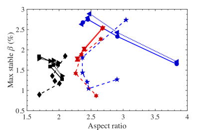
Figure 7: Maximum stable $\beta$ plotted against aspect ratio for each of the test configurations. Symbols are as defined in the legend in Fig. 4.

Characteristics of the high-$\beta$ equilibrium are shown in Fig. 8. Figs. 8a-c compare the plasma geometry for $\beta=3.0\%$ to the vacuum configuration ($\beta=0$). Due to the sign change of the bootstrap current profile (Fig. 8d), the radial shifts of the axis and the boundary are in opposite directions (Fig. 8c). The toroidal current significantly affects the rotational transform profile near the axis (Fig. 8e) but less so near the edge.

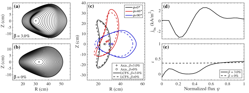
Figure 8: Properties of the high-$\beta$ equilibrium attained with $I_{IL}/I_{PF}$ = 3.25, $\theta_{\text{tilt}}=78^{\circ}$, and the hollow pressure profile. (a) Flux surfaces for the equilibrium with $\beta$ = 3.0%. (b) Flux surfaces for the same configuration with $\beta$ = 0%. (c) Boundaries for the equilibrium with $\beta$ = 3.0% (solid lines) compared with boundaries calculated with $\beta=0$ (dashed lines) for three different poloidal cross-sections. (d) Profile of toroidal current (i.e., the calculated bootstrap current). (e) Profile of rotational transform with $\beta$ = 3.0% (solid line) and $\beta$ = 0% (dashed line).

Corresponding characteristics of the least stable configuration are shown in Fig. 9. The differences in flux surface geometry (Fig. 9a-c) and rotational transform (Fig. 9e) from the high-$\beta$ configuration result primarily from the different $\theta_{\text{tilt}}$ and $I_{IL}/I_{PF}$. The lower magnitude of the bootstrap current (Fig. 9d), as well as the smaller excursion of $\iota$ from its vacuum values (Fig. 9e), are consistent with the lower pressure.

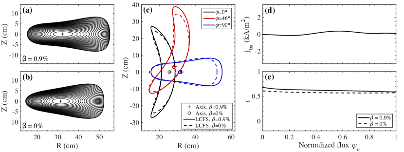
Figure 9: Like Fig. 8, but for the least stable equilibrium ($\beta=0.9\%$), attained with $I_{IL}/I_{PF}$ = 2.75, $\theta_{\text{tilt}}=88^{\circ}$, and peaked pressure profile.

It should be noted that perfect stellarator symmetry was assumed for the calculations here for computational simplicity. However, it is known that CNT’s coils have significant misalignments and exhibit field errors that break the two-field-period stellarator symmetry.Hammond et al. (2016a) The principal effect of these errors was shown to be an offset of the rotational transform profiles associated with each setting of $I_{IL}/I_{PF}$. Hence, incorporating CNT’s field errors is expected to result in an offset of the plots shown in Fig. 4 along the abscissa.

VI Heating power requirements

The heating power requirements for the scenarios outlined in the previous section can be roughly estimated as follows stellarator scaling laws.

We estimate $\beta$ asChen (1986)

$$\beta=\frac{n_{e}k_{B}T_{e}+n_{i}k_{B}T_{i}}{B^{2}/2\mu_{0}}.$$ (1)

Here, $n_{e}$ and $n_{i}$ are the electron and ion densities (assuming a single dominant ion species), $T_{e}$ and $T_{i}$ are the electron and ion temperatures, $k_{B}$ is Boltzmann’s constant, $B$ is the magnetic field, and $\mu_{0}$ is the vacuum permeability. We assume a quasi-neutral plasma with $n_{e}=n_{i}$ and, as in Sec. III, $T_{i}=0.3T_{e}$. Hence, the numerator of Eq. 1 simplifies to $1.3n_{e}k_{B}T_{e}$. This, in turn, may be re-expressed in terms of heating power $P$ as $1.3(\tau_{E}P/V)$, where $V$ is the plasma volume and where $\tau_{E}$ is the energy confinement time.

We estimate $\tau_{E}$ using the 2004 International Stellarator Scaling law (ISS04):Yamada et al. (2005)

$$\tau_{\text{E,ISS04}}=0.134f_{\text{ren}}a^{2.28}R^{0.64}P^{-0.61}\bar{n}_{e}^{0.54}B^{0.84}\text{\sout{$\iota$}}_{2/3}^{0.41}$$ (2)

Here $R$ and $a$ are the plasma major and minor radius in meters, $B$ is the magnetic field in Tesla, and $\text{\sout{$\iota$}}_{2/3}$ is the rotational transform evaluated at two-thirds the minor radius of the LCFS. The heating power $P$ (in MW in this formula) is treated as an independent variable. Incidentally, the ISS04 dataset involved several heliotrons/torsatrons and one device with circular coils (the TJ-II heliac). Also note that CNT is essentially a heliotron/torsatron (not a classical stellarator) with two ($\ell=2$) “helical” coils of poloidal number $m=1$ and toroidal number $n=1$ which, in effect, are circular. It should be noted that the values of $R$, $B$, and line-averaged electron density $\bar{n}_{e}$ (in units of $10^{19}~{}\text{m}^{-3}$), are lower in CNT than in other devices which $\tau_{\text{E,ISS04}}$ is based upon. Said otherwise, the scaling law is being extrapolated here. Furthermore, $\tau_{\text{E,ISS04}}$ is determined based on current-free or nearly current-free plasmas, whereas the high-$\beta$, low-aspect-ratio equilibria evaluated in this paper contain a small but finite bootstrap current.

The renormalization coefficient, $f_{\text{ren}}$, is a device-specific fitting parameter. Among the stellarators in the ISS04 database, this value ranged from 0.25 for TJ-II to unity for a configuration of W7-AS. This parameter has not been calculated for CNT. However, it was observed that the parameter was inversely correlated with the toroidal effective ripple, $\epsilon_{\text{eff}}$. This tendency follows from the association of greater ripple with a larger population of helically trapped particles. In particular, $\epsilon_{\text{eff}}(2/3)$ (evaulated at two-thirds of the minor radius) was found to relate to $f_{\text{ren}}$ roughly as $f_{\text{ren}}\propto\epsilon_{\text{eff}}(2/3)^{-0.4}$ for values of $\epsilon_{\text{eff}}(2/3)$ between 0.02 and 0.4 (see Fig. 7 in Ref. Yamada et al. (2005)). For CNT, a value of $\epsilon_{\text{eff}}(2/3)$ of 1.6 was calculated for the configuration $\theta_{\text{tilt}}=64^{\circ}$, $I_{IL}/I_{PF}=4.22$. Seiwald et al. (2007). Extrapolating the relationship observed in the ISS04 database to the range of $\epsilon_{\text{eff}}$ for CNT, we posit $f_{\text{ren}}\approx(0.25\pm 0.05)\epsilon_{\text{eff}}(2/3)^{-0.4}$, leading to an estimate of $f_{\text{ren}}=0.21$ for CNT with upper and lower bounds of 0.25 and 0.17, respectively.

$\tau_{E}$ is evaluated in two main regimes of electron density density $\bar{n}_{e}$. The first is the highest attainable before the plasma radiatively collapses, determined through a formula derived by Sudo,Sudo et al. (1990)

$$n_{\text{Sudo}}=2.5\sqrt{\frac{PB}{a^{2}R}}.$$ (3)

A similar formula was derived at W7-AS Giannone et al. (2003) and yields similar results, not shown for brevity. The second is the cutoff density above which microwaves for ECH cannot propagate. For heating at the fundamental harmonic in the ordinary mode at frequency $\omega_{\text{rf}}=2\pi\times 2.45$ GHz, this is

$$n_{\text{co,O}}=\frac{\epsilon_{0}m_{e}}{e^{2}}{\omega_{\text{rf}}}^{2}.$$ (4)

For heating at the second harmonic in the extraordinary mode using the same heating frequency (and, therefore, half the field), the highest density at which propagation may occur throughout the plasma corresponds to the right-handed cutoff, effectively half of the ordinary-mode cutoff:

$$n_{\text{co,X2}}=\frac{1}{2}\frac{\epsilon_{0}m_{e}}{e^{2}}{\omega_{\text{rf}}}^{2};$$ (5)

Results of these calculations for the high-$\beta$ and least stable configurations are shown in Fig. 10. The three black curves shown in each plot, from top to bottom, give the value of $\beta$ determined using Eqs. 1-2, with densities from Eqs. 3, 4, and 5, respectively. Thus, the blue-shaded region below the curve for $\beta(n_{\text{co,O}})$ is accessible by underdense plasmas, and the red-shaded region between $\beta(n_{\text{co,O}})$ and $\beta(n_{\text{Sudo}})$ corresponds to $\beta$ values that are accessible with overdense microwave heating.

The red lines in Fig. 10a-b are $(P,\beta)$ contours corresponding to $T_{e}=30$ eV, determined by inverting Eqs. 1 and 2. To the left of these lines, $T_{e}$ is lower; to the right, $T_{e}$ is higher. Thus, to obtain $\beta=3.0\%$ in the high-$\beta$ configuration while maintaining a minimum $T_{e}$ of 30 eV, about 1.8 MW of power will be needed (Fig. 10a). To obtain $\beta=0.9\%$ in the least stable configuration at $T_{e}=30$ eV, about 60 kW will be needed. It should be noted, however, that these estimates are sensitive to $f_{\text{ren}}$ (Eq. 2). If these estimates are redone using the upper and lower bounds mentioned above ($0.17<f_{\text{ren}}<0.25$), a range of 1 to 3 MW is established for the high-$\beta$ configuration and 40 to 100 kW for the least stable configuration.

Both configurations fall within the overdense region for heating with 2.45 GHz and will therefore both require overdense microwave heating. The parameters of these configurations are compared with present experimental conditions in Table 1. Note that $\text{\sout{$\iota$}}_{2/3}$ for the least stable configuration exceeds that of the high-$\beta$ configuration by a factor of nearly 7. This corresponds to a factor of 2 increase in $\tau_{\text{E}}$ (Eq. 2) due to $\text{\sout{$\iota$}}_{2/3}$ alone. This, combined with the reduced $\beta$, explains why so much less power is required for the least stable configuration.

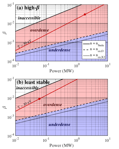
Figure 10: Accessible $\beta$ at different levels of heating power according to stellarator scaling laws for (a) the high-$\beta$ configuration and (b) the least stable configuration. Values of $\beta$ above the solid line are considered inaccessible because the plasma density exceeds the Sudo limit. Values below the dashed line correspond to plasmas underdense to 2.45 GHz ECH in the ordinary mode; values between the solid and dashed lines could be attainable by overdense heating. The red lines are contours of $T_{e}=30$ eV in the $(P,\beta)$ parameter space. The red circles indicate the power levels needed to attain the maximum ballooning-stable $\beta$ in each configuration.

Parameter	Present	Least stable	High-$\beta$
$\theta_{\text{tilt}}$ (deg)	78	88	78
$a$ (m)	0.14	0.12	0.13
$R$ (m)	0.31	0.30	0.32
$P$ (kW)	0.5-8	40-100	1,000-3,000
$n_{e}$ ($10^{17}~{}\text{m}^{-3}$)	0.5-3	50	200
$B$ (T)	0.08	0.08	0.08
$\text{\sout{$\iota$}}_{2/3}$	0.36	0.62	0.09
$T_{e}$ (eV)	4-8	30	30

Table 1: Comparison of present CNT experimental parameters with those of the least stable and high-$\beta$ configurations.

VII Conclusions and future work

The foregoing work has established that ballooning-stable equilibria with average $\beta$ values of up to 3.0% should be attainable in CNT, and possibly even higher, as the ballooning stability limit was not found for some configurations (Fig. 4a). Here it was assumed that the plasma current is dominated by the bootstrap current. The limitations on stability depend on the magnetic configuration, with the $\theta_{\text{tilt}}=78^{\circ}$ coil orientation capable of the highest $\beta$. Stability also depends on the pressure profile and the associated bootstrap current profile: plasmas with peaked pressure profiles, for the same $\theta_{\text{tilt}}$ and $I_{IL}/I_{PF}$, may become unstable at $\beta\simeq 1.4\%$. These stability limits are lower than in other stellarators, and thus more easily accessible. Stellarator scaling laws indicate that a 30 eV plasma with $\beta=3.0\%$ might be attainable with 2.45 GHz microwaves at a power of 1-3 MW if overdense heating mechanisms are employed. Furthermore, a configuration was found that may become ballooning-unstable at $\beta$ as low as 0.9%, which would be attainable at a power of 40-100 kW.

A self-consistent estimate of the maximum stable $\beta$ would require that, instead of the normalized profiles in Fig. 3 based on 10 kW heating experiments, we use for the stability calculations a pressure profile as close as possible to what we would obtain with higher heating power. In turn, this would require full-wave and Fokker-Planck modeling, which is left as future work. A ray- or beam-tracing would not be appropriate due to the spatial scales of the problem (i.e., the plasma minor radius is similar to the microwave vacuum wavelength).

Finally, indications of a second region of stability were found in Figs. 5-6, which will deserve more extensive modeling and experimentation in the future.

References

- Weller et al. (2003) A. Weller, J. Geiger, A. Werner, M. C. Zarnstorff, C. Nührenberg, E. Sallander, J. Baldzuhn, R. Brakel, R. Burhenn, A. Dinklage, E. Fredrickson, F. Gadelmeier, L. Gianonne, P. Grigull, D. Hartmann, R. Jaenicke, S. Klose, J. P. Knauer, A. Könies, Y. I. Kolesnichenko, H. P. Laqua, V. V. Lutsenko, K. McCormick, D. Monticello, M. Osakakabe, E. Pasch, A. Reiman, N. Rust, D. A. Spong, F. Wagner, Y. V. Yakovenko, the W7-AS Team, and NBI-Group, Plasma Physics and Controlled Fusion 45, A285 (2003).
- Sakakibara et al. (2015) S. Sakakibara, K. Y. Watanabe, Y. Takemura, M. Okamoto, S. Ohdachi, Y. Suzuki, Y. Narushima, K. Ida, M. Yoshinuma, K. Tanaka, T. Tokuzawa, I. Yamada, H. Yamada, Y. Takeiri, and the LHD Experiment Group, Nuclear Fusion 55, 083020 (2015).
- Cuthbert et al. (1998) P. Cuthbert, J. L. V. Lewandowski, H. J. Gardner, M. Persson, D. B. Singleton, R. L. Dewar, N. Nakajima, and W. A. Cooper, Physics of Plasmas 5, 2921 (1998).
- Hegna and Nakajima (1998) C. C. Hegna and N. Nakajima, Physics of Plasmas 5, 1336 (1998).
- Hudson and Hegna (2003) S. R. Hudson and C. C. Hegna, Physics of Plasmas 10, 4716 (2003).
- Hudson and Hegna (2004) S. R. Hudson and C. C. Hegna, Physics of Plasmas 11, L53 (2004).
- Rafiq et al. (2010) T. Rafiq, C. C. Hegna, J. D. Callen, and A. H. Kritz, Physics of Plasmas 17, 022502 (2010).
- Nielson et al. (2000) G. H. Nielson, A. H. Reiman, M. C. Zarnstorff, A. Brooks, G.-Y. Fu, R. J. Goldston, L.-P. Ku, Z. Lin, R. Majeski, D. A. Monticello, H. Mynick, N. Pomphrey, M. H. Redi, W. T. Reierson, J. A. Schmidt, S. P. Hirshman, J. F. Lyon, L. A. Berry, B. E. Nelson, R. Sanchez, D. A. Spong, A. H. Boozer, W. H. Miner Jr., P. M. Valanju, W. A. Cooper, M. Drevlak, P. Merkel, and C. Nührenberg, Physics of Plasmas 7, 1911 (2000).
- Weller et al. (2001) A. Weller, M. Anton, J. Geiger, M. Hirsch, R. Jaenicke, A. Werner, C. Nührenberg, E. Sallander, D. A. Spong, and the W7-AS team, Physics of Plasmas 8, 931 (2001).
- Beidler et al. (2001) C. D. Beidler, E. Harmeyer, F. Herrnegger, Y. Igitkhanov, A. Kendl, J. Kisslinger, Y. I. Kolesnichenko, V. V. Lutsenko, C. Nührenberg, I. Sidorenko, E. Strumberger, H. Wobig, and Y. V. Yakovenko, Nuclear Fusion 41, 1759 (2001).
- Sagara, Igitkhanov, and Najmabadi (2010) A. Sagara, Y. Igitkhanov, and F. Najmabadi, Fusion Engineering and Design 85, 1336 (2010).
- Pedersen et al. (2004) T. S. Pedersen, A. H. Boozer, J. P. Kremer, R. G. Lefrancois, W. T. Reiersen, F. D. Dahlgren, and N. Pomphrey, Fusion Sci. Technol. 46, 200 (2004).
- Pedersen et al. (2006) T. S. Pedersen, J. P. Kremer, R. G. Lefrancois, Q. Marksteiner, X. Sarasola, and N. Ahmad, Phys. Plasmas 13, 012502 (2006).
- Kremer et al. (2006) J. P. Kremer, T. S. Pedersen, R. G. Lefrancois, and Q. Marksteiner, Phys. Rev. Lett. 97, 095003 (2006).
- Sarasola and Pedersen (2012) X. Sarasola and T. S. Pedersen, Plasma Phys. Controlled Fusion 54, 124008 (2012).
- Hammond et al. (2016a) K. C. Hammond, A. Anichowski, P. W. Brenner, T. S. Pedersen, S. Raftopoulos, P. Traverso, and F. A. Volpe, Plasma Physics and Controlled Fusion 58, 074002 (2016a).
- Hammond et al. (2016b) K. C. Hammond, R. R. Diaz-Pacheco, Y. Kornbluth, F. A. Volpe, and Y. Wei, Review of Scientific Instruments 87, 11E119 (2016b).
- Hirshman and Whitson (1983) S. P. Hirshman and J. C. Whitson, Physics of Fluids 26, 3553 (1983).
- Sanchez et al. (2000) R. Sanchez, S. Hirshman, J. Whitson, and A. Ware, Journal of Computational Physics 161, 576 (2000).
- Hirshman, van Rij, and Merkel (1986) S. P. Hirshman, W. I. van Rij, and P. Merkel, Computer Physics Communications 43, 143 (1986).
- Weller et al. (2006) A. Weller, S. Sakakibara, K. Y. Watanabe, K. Toi, J. Geiger, M. C. Zarnstorff, S. R. Hudson, A. Reiman, A. Werner, C. Nührenberg, S. Ohdachi, Y. Suzuki, H. Yamada, the W7-AS team, and the LHD team, Fusion Science and Technology 50, 158 (2006).
- Moroz (1996) P. E. Moroz, Physics of Plasmas 3, 3055 (1996).
- Shaing et al. (1989) K. C. Shaing, E. C. Crume, J. S. Tolliver, S. P. Hirshman, and W. I. van Rij, Physics of Fluids B 1, 148 (1989).
- Post et al. (1977) D. E. Post, R. V. Jensen, C. B. Tarter, W. H. Grasberger, and W. A. Lokke, in Atomic Data and Nuclear Data Tables, Vol. 20 (Academic Press, Inc., 1977) pp. 397–439.
- Greene and Chance (1981) J. M. Greene and M. S. Chance, Nuclear Fusion 21, 453 (1981).
- Gryaznevich et al. (1998) M. Gryaznevich, R. Akers, P. G. Carolan, N. J. Conway, D. Gates, A. R. Field, T. C. Hender, I. Jenkins, R. Martin, M. P. S. Nightingale, C. Ribeiro, D. C. Robinson, A. Sykes, M. Tournianski, M. Valovič, and M. J. Walsh, Physical Review Letters 80, 3972 (1998).
- Chen (1986) F. F. Chen, Introduction to Plasma Physics and Controlled Fusion, 2nd ed. (Plenum Press, New York, NY, 1986).
- Yamada et al. (2005) H. Yamada, J. H. Harris, A. Dinklage, E. Ascasibar, F. Sano, S. Okamura, J. Talmadge, U. Stroth, A. Kus, S. Murakami, M. Yokoyama, C. D. Beidler, V. Tribaldos, K. Y. Watanabe, and Y. Suzuki, Nuclear Fusion 45, 1684 (2005).
- Seiwald et al. (2007) B. Seiwald, V. V. Nemov, T. S. Pedersen, and W. Kernbichler, Plasma Physics and Controlled Fusion 49, 2063 (2007).
- Sudo et al. (1990) S. Sudo, Y. Takeiri, H. Zushi, F. Sano, K. Itoh, K. Kondo, and A. IIyoshi, Nuclear Fusion 30, 11 (1990).
- Giannone et al. (2003) L. Giannone, R. Brakel, R. Burhenn, H. Ehmler, Y. Feng, P. Grigull, K. McCormick, F. Wagner, J. Baldzuhn, Y. Igitkhanov, J. Knauer, K. Nishimura, E. Pasch, B. J. Peterson, N. Ramasubramanian, N. Rust, A. Weller, A. Werner, and the W7-AS Team, Plasma Physics and Controlled Fusion 45, 1713 (2003).