Light-front $\phi_{2}^{4}$ theory with sector-dependent mass

Abstract

As an extension of recent work on two-dimensional light-front $\phi^{4}$ theory, we implement Fock-sector dependence for the bare mass. Such dependence should have important consequences for the convergence of nonperturbative calculations with respect to the level of Fock-space truncation. The truncation forces the self-energy corrections to be sector-dependent; in particular, the highest sector has no self-energy correction. Thus, the bare mass can be considered sector dependent as well. We find that, although higher Fock sectors have a larger probability, the mass of the lightest state and the value of the critical coupling are not significantly affected. This implies that coherent states or the light-front coupled-cluster method may be required to properly represent critical behavior.

I Introduction

In a recent calculation phi4sympolys , two-dimensional $\phi^{4}$ theory was solved for the lowest mass eigenstates of the light-front Hamiltonian. The eigenstates were represented by truncated Fock-state expansions, with momentum-space wave functions as the coefficients. This work included estimation of the critical coupling, where the $\phi\rightarrow-\phi$ symmetry of the theory is broken Chang . At this critical coupling, one would expect that the probabilities for the higher Fock sectors, computed as integrals of the squares of the Fock wave functions, would increase dramatically. In particular, the probability for the one-particle sector of the lowest massive state should go to zero. This was not observed.

The expectation that the one-particle probability would go to zero is important for the calculation of the connection between equal-time RychkovVitale ; LeeSalwen ; Sugihara ; SchaichLoinaz ; Bosetti ; Milsted and light-front estimates phi4sympolys ; VaryHari of the critical coupling. This is determined by the relationship between the different mass renormalizations in the two quantizations SineGordon , which is fixed by tadpole contributions computed from the vacuum expectation value of $\phi^{2}$. The behavior of this vacuum expectation value is dominated by the product of the one-particle probability times the logarithm of the mass phi4sympolys . The mass goes to zero at the critical coupling, making zero probability a necessity for a finite result.

In the previous work, the explanation proposed for this apparent paradox was that the calculation did not use sector-dependent bare masses. This meant that the highest Fock sector kept in the calculation used a fixed bare mass even as the eigenstate mass approached zero. Excitation of such Fock states is then very unlikely.

The use of sector-dependent bare parameters, or ‘sector-dependent renormalization’ as it is usually called, has a long history SecDep-Wilson ; HillerBrodsky ; Karmanov . A Fock-space truncation forces self-energy corrections and vertex corrections to be different in different Fock sectors. This makes sector-dependent counterterms a natural choice. In addition, the truncation causes divergences that would have been canceled by contributions from higher Fock states that are now absent. Sector-dependent counterterms can take these divergences into account. However, in at least some theories, the sector-dependent bare couplings can lead to inconsistencies in the interpretation of wave functions and Fock-sector probabilities SecDep . Thus, use of sector-dependent bare masses can be a compromise. Of course, for two-dimensional $\phi^{4}$ theory, divergences are not the issue, and it is only near the critical coupling where sector-dependent masses could be a useful approximation, as already indicated by some preliminary work LFCCphi4 .

The use of light-front quantization LFreviews is important for its simple vacuum and well-defined Fock state expansions as well as for the separation of relative and external momenta. We define light-front coordinates Dirac as $x^{\pm}=t\pm z$, with $x^{+}$ the light-front time. The light-front energy is then $p^{-}=E-p_{z}$, and the light-front momentum is $p^{+}=E+p_{z}$. In what follows, we will drop the superscript from $p^{+}$ to simplify the notation. The inner product between momentum and position is $p\cdot x=\frac{1}{2}(p^{-}x^{+}+px^{-})$, and the mass-shell condition is $p^{-}=m^{2}/p$. The light-front Hamiltonian eigenvalue problem is then ${\cal P}^{-}|\psi(P)\rangle=\frac{M^{2}}{P}|\psi(P)\rangle$, with $|\psi(P)\rangle$ the eigenstate with mass $M$ and light-front momentum $P$. The eigenstate is expanded in a set of Fock states, which converts the formal eigenvalue problem into a system of equations for the Fock-state wave functions. Numerical approximations then transform this system into a matrix eigenvalue problem. Our chosen numerical approximation is an expansion of the wave functions in terms of symmetric multivariate polynomials GenSymPolys .

The content of the remainder of the paper is as follows. Section II provides a brief introduction to $\phi^{4}$ theory and formulates the system of equations for the Fock-state wave functions. These equations are modified in Sec. III to accommodate a sector-dependent bare mass; the results from their solution are presented and discussed. The work is summarized briefly in Sec. IV. Details of the numerical methods are left to an Appendix.

II Light-front $\phi^{4}$ theory

The Lagrangian for $\phi^{4}$ theory is

$${\cal L}=\frac{1}{2}(\partial_{\mu}\phi)^{2}-\frac{1}{2}\mu^{2}\phi^{2}-\frac{\lambda}{4!}\phi^{4},$$ (1)

with $\mu$ the bare mass. The light-front Hamiltonian density is

$${\cal H}=\frac{1}{2}\mu^{2}\phi^{2}+\frac{\lambda}{4!}\phi^{4}.$$ (2)

The field $\phi$ is expanded in terms of creation and annihilation operators $a^{\dagger}(p)$ and $a(p)$ as

$$\phi(x^{+}=0,x^{-})=\int\frac{dp}{\sqrt{4\pi p}}\left\{a(p)e^{-ipx^{-}/2}+a^{\dagger}(p)e^{ipx^{-}/2}\right\}.$$ (3)

The operators obey the commutation relation

$$[a(p),a^{\dagger}(p^{\prime})]=\delta(p-p^{\prime}).$$ (4)

Substitution of the mode expansion and integration of the Hamiltonian density with respect to $x^{-}$ yields the light-front Hamiltonian ${\cal P}^{-}={\cal P}^{-}_{11}+{\cal P}^{-}_{22}+{\cal P}^{-}_{13}+{\cal P}^{-}_{31}$, with

$${\cal P}^{-}_{11} = \int dp\frac{\mu^{2}}{p}a^{\dagger}(p)a(p),$$ (5)

$${\cal P}^{-}_{22} = \frac{\lambda}{4}\int\frac{dp_{1}dp_{2}}{4\pi\sqrt{p_{1}p_{2}}}\int\frac{dp^{\prime}_{1}dp^{\prime}_{2}}{\sqrt{p^{\prime}_{1}p^{\prime}_{2}}}\delta(p_{1}+p_{2}-p^{\prime}_{1}-p^{\prime}_{2})a^{\dagger}(p_{1})a^{\dagger}(p_{2})a(p^{\prime}_{1})a(p^{\prime}_{2}),$$ (6)

$${\cal P}^{-}_{13} = \frac{\lambda}{6}\int\frac{dp_{1}dp_{2}dp_{3}}{4\pi\sqrt{p_{1}p_{2}p_{3}(p_{1}+p_{2}+p_{3})}}a^{\dagger}(p_{1}+p_{2}+p_{3})a(p_{1})a(p_{2})a(p_{3}),$$ (7)

$${\cal P}^{-}_{31} = \frac{\lambda}{6}\int\frac{dp_{1}dp_{2}dp_{3}}{4\pi\sqrt{p_{1}p_{2}p_{3}(p_{1}+p_{2}+p_{3})}}a^{\dagger}(p_{1})a^{\dagger}(p_{2})a^{\dagger}(p_{3})a(p_{1}+p_{2}+p_{3}).$$ (8)

The eigenstate of ${\cal P}^{-}$, with eigenvalue $M^{2}/P$, can be expressed as an expansion

$$|\psi(P)\rangle=\sum_{m}P^{\frac{m-1}{2}}\int\prod_{i}^{m}dy_{i}\delta(1-\sum_{i}^{m}y_{i})\psi_{m}(y_{i})|y_{i};P,m\rangle$$ (9)

in terms of Fock states

$$|y_{i};P,m\rangle=\frac{1}{\sqrt{m!}}\prod_{i=1}^{m}a^{\dagger}(y_{i}P)|0\rangle,$$ (10)

where the coefficient $\psi_{m}$ is the wave function for the Fock sector with $m$ constituents. The wave function depends on the momentum fractions $y_{i}\equiv p_{i}/P$, which are boost invariant, unlike the individual momenta $p_{i}$. The leading factor of $P^{\frac{m-1}{2}}$ allows the normalization of the wave functions to be independent of $P$; we require $\langle\psi(P^{\prime})|\psi(P)\rangle=\delta(P-P^{\prime})$, which yields

$$1=\sum_{m}\int\prod_{i}^{m}dy_{i}\delta(1-\sum_{i}^{m}y_{i})|\psi_{m}(y_{i})|^{2}.$$ (11)

The probability of the $m$th Fock sector is then just $\int\prod_{i}^{m}dy_{i}\delta(1-\sum_{i}^{m}y_{i})|\psi_{m}(y_{i})|^{2}$. Because the Hamiltonian changes particle number by zero or two, never an odd number, the sum over Fock sectors is either even or odd, depending on which state is chosen as the lowest Fock state. We will focus on the odd case.

The eigenvalue problem becomes a coupled system of equations for the wave functions:

$$\sum_{i}^{m}\frac{\mu^{2}}{y_{i}}\psi_{m}(y_{i})+\frac{\lambda}{4\pi}\frac{m(m-1)}{4\sqrt{y_{1}y_{2}}}\int\frac{dx_{1}dx_{2}}{\sqrt{x_{1}x_{2}}}\delta(y_{1}+y_{2}-x_{1}-x_{2})\psi_{m}(x_{1},x_{2},y_{3},\ldots,y_{m})$$ (12)

$$+\frac{\lambda}{4\pi}\frac{m}{6}\sqrt{(m+2)(m+1)}\int\frac{dx_{1}dx_{2}dx_{3}}{\sqrt{y_{1}x_{1}x_{2}x_{3}}}\delta(y_{1}-x_{1}-x_{2}-x_{3})\psi_{m+2}(x_{1},x_{2},x_{3},y_{2},\ldots,y_{m})$$

$$+\frac{\lambda}{4\pi}\frac{m-2}{6}\frac{\sqrt{m(m-1)}}{\sqrt{y_{1}y_{2}y_{3}(y_{1}+y_{2}+y_{3})}}\psi_{m-2}(y_{1}+y_{2}+y_{3},y_{4},\ldots,y_{m})=M^{2}\psi_{m}(y_{i}).$$

This is an infinite system and requires some form of truncation before a numerical solution can be attempted. The standard truncation is a Fock-space truncation to some maximum number of constituents $N_{\rm max}$. However, as discussed in the Introduction, this causes self-energy contributions to become sector-dependent. For the sector with $m=N_{\rm max}$, there is no self-energy because no loop corrections are allowed; any intermediate states would have more than $N_{\rm max}$ constituents. Therefore, the bare mass in the top sector is reasonably equal to the physical mass $M$ of the lowest state. As we step down from the top sector, the complexity of the self-energy contributions steadily increases, and the bare mass can be adjusted to compensate.

III Sector-dependent mass

To implement a sector-dependent bare mass, we replace $\mu$ in the first term of (12) by $\mu_{m}$ and compute the $\mu_{m}$ for a given eigenmass $M$ by steadily increasing $N_{\rm max}$. For $N_{\rm max}=1$, we have immediately that $\mu_{1}=M$ and $|\psi(P)\rangle=a^{\dagger}(P)|0\rangle$. For $N_{\rm max}=3$, we set $\mu_{3}=M$ and solve the following two equations for $\mu_{1}$ and $\psi_{3}/\psi_{1}$:

$$\mu_{1}^{2}\psi_{1}+\frac{\lambda}{4\pi}\frac{1}{\sqrt{6}}\int\frac{dx_{1}dx_{2}dx_{3}}{\sqrt{x_{1}x_{2}x_{3}}}\delta(1-x_{1}-x_{2}-x_{3})\psi_{3}(x_{1},x_{2},x_{3})=M^{2}\psi_{1}$$ (13)

$$\sum_{i}^{3}\frac{M^{2}}{y_{i}}\psi_{3}(y_{1},y_{2},y_{3}) + \frac{\lambda}{4\pi}\frac{3}{2\sqrt{y_{1}y_{2}}}\int\frac{dx_{1}dx_{2}}{\sqrt{x_{1}x_{2}}}\delta(y_{1}+y_{2}-x_{1}-x_{2})\psi_{3}(x_{1},x_{2},y_{3})$$ (14)

$$+\frac{\lambda}{4\pi}\frac{1}{\sqrt{6}}\frac{1}{\sqrt{y_{1}y_{2}y_{3}}}\psi_{1}=M^{2}\psi_{3}(y_{1},y_{2},y_{3}).$$

For $N_{\rm max}=5$, we set $\mu_{3}$ to the value of $\mu_{1}$ obtained for $N_{\rm max}=3$, set $\mu_{5}=M$, and solve a system of three equations for $\mu_{1}$, $\psi_{3}/\psi_{1}$, and $\psi_{5}/\psi_{1}$. We continue in this manner until $\mu_{1}$ has converged with respect to the Fock-space truncation fixed by $N_{\rm max}$.

As described in the Appendix, the equations are solved numerically, with the wave functions expanded in a polynomial basis GenSymPolys . The principal result of the calculation is the plot of the eigenvalues versus coupling strength in Fig. 1. These values are extrapolated in the polynomial basis size for each Fock sector, and the Fock-space truncation is varied from $N_{\rm max}=3$ to 9. With respect to the Fock-space truncations, the results converge, in an oscillatory fashion, to within the numerical error at a given truncation.

Figure 1: Lowest mass eigenvalue for odd numbers of constituents for different Fock-space truncations to three (circles), five (triangles), seven (diamonds), and nine (hexagons) constituents. The values of $M^{2}/\mu^{2}$ and $g\equiv\lambda/(4\pi\mu^{2})$ are obtained as extrapolations in the orders of basis polynomials, and the error bars estimate the range of fits for the extrapolations.

These results are consistent with those from the standard parameterization, with no sector dependence in the bare mass, as reported in phi4sympolys . This can be seen in Fig. 2, where the previous results are added to the plot from Fig. 1. The critical coupling, as indicated by the point where $M^{2}$ reaches zero, is again estimated to be 2.1. The sector-dependent results do converge more slowly; they require $N_{\rm max}=9$ compared to the $N_{\rm max}=5$ required for the standard parameterization. This is to be expected, even desired, because we expect that higher Fock states should become more important as the critical coupling is approached.

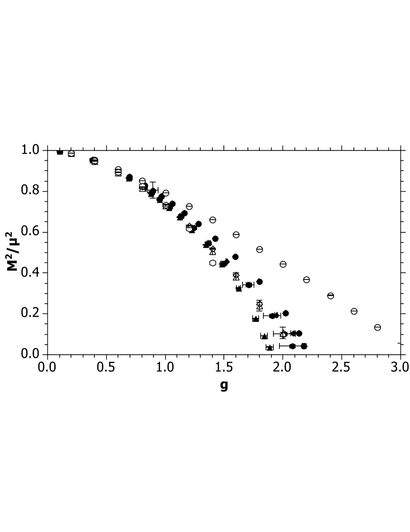
Figure 2: Same as Fig. 1, but with the standard parameterization results (open circles, triangles, and diamonds) of phi4sympolys , which include up to seven constituents, and the light-front coupled cluster results (open hexagons) of LFCCphi4 added for comparison. Without sector-dependent masses, the Fock state expansion converges more quickly, and the five and seven-constituent results are nearly identical, between themselves and with the nine-constituent sector-dependent results.

To understand what might be happening in the structure of the eigenstate, we plot the relative Fock-sector probabilities in Fig. 3. These are computed as $\int\prod_{i}^{m}dy_{i}\delta(1-\sum_{i}^{m}y_{i})|\psi_{m}(y_{i})|^{2}/|\psi_{1}|^{2}$, for both the sector-dependent and standard parameterizations. In the former case, $N_{\rm max}=9$ and in the latter, $N_{\rm max}=7$. For the sector-dependent calculations, results do not extend beyond the critical coupling, because negative $M^{2}$ is ill-defined for sector-dependent renormalization; the bare mass in the highest Fock sector would then be imaginary. The relative probabilities are essentially the same in the three-body Fock sector, indicating full convergence with respect to the Fock-space truncation. In Fock sectors with five and seven constituents, the relative probability for the sector-dependent case rises above the probability in the standard case as the critical coupling is approached. The greater probability is expected; however, the full expectation was that these probabilities would have a much more striking increase. In fact, as relative probabilities, they will tend to infinity as the one-body probability $|\psi_{1}|^{2}$ goes to zero, and obviously this is not happening, and the original hypothesis, that sector-dependent bare masses would resolve the paradox, must be incorrect.

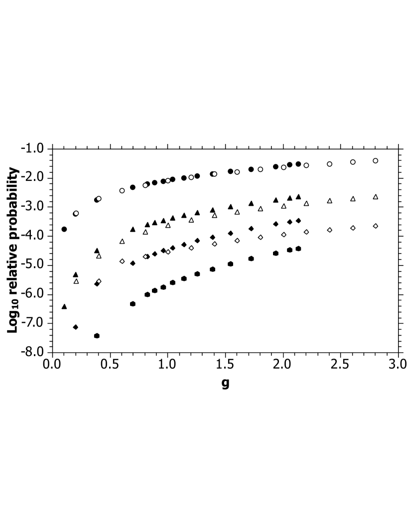
Figure 3: Relative Fock-sector probabilities for the three, five, seven and nine-constituent sectors when the truncation is $N_{\rm max}=9$.

The finite one-body probability also prevents any improvement in the calculation of the difference in mass renormalization between equal-time and light-front quantization, as attempted in phi4sympolys . Therefore, no new calculation is attempted here.

IV Summary

Contrary to expectations, we have found that a sector-dependent bare mass does not provide any significant improvement in the solution of $\phi_{2}^{4}$ theory. The sector dependence does allow higher Fock states to have a larger contribution, but the contribution to the lowest massive state is not large in an absolute sense, and the one-body contribution remains dominant, even at the critical coupling. Convergence of the bare mass in the lowest sectors, as the Fock-space truncation is relaxed, is quite rapid, as can be seen in Fig. 4.

There is, however, a hint as to what might be needed in earlier work LFCCphi4 that explored the light-front coupled-cluster (LFCC) method LFCC . In this method, all of the higher Fock states are kept. To keep the calculation finite in size, the relationship between Fock wave functions is truncated, so that wave functions of the higher Fock states are related to those of the lower states in a simple way. The wave functions are then determined by a nonlinear equation that sums over contributions from all Fock states. In this calculation, a relative probability shows a rapid increase, in Fig. 5 of LFCCphi4 , although at an unexpected value of the coupling. The hint is that coherent effects across all of Fock space are important, something that ordinary Fock-space truncation would not be able to reproduce. That this would happen at the phase transition to broken symmetry is actually not surprising.

Appendix A Numerical methods

The coupled system (12), modified to use sector-dependent masses, is solved numerically, with each wave function expanded in a basis of symmetric multivariate polynomials GenSymPolys $P_{ki}^{(m)}(y_{1},\ldots,y_{m})$. Here $k$ is the order and $m$ the number of momentum fractions; the index $i$ differentiates between linearly independent polynomials of the same order. The expansion for a wave function is

$$\psi_{m}(y_{1},\ldots,y_{m})=\sqrt{y_{1}y_{2}\cdots y_{m}}\sum_{ni}c_{ni}^{(m)}P_{ni}^{(m)}(y_{1},\ldots,y_{m})$$ (15)

Projection of the system of equations onto the basis functions then yields a system of matrix equations

$$\tilde{\mu}_{m}^{2}\sum_{n^{\prime}i^{\prime}}\left[T^{(m)}_{ni,n^{\prime}i^{\prime}}+V^{(m,m)}_{ni,n^{\prime}i^{\prime}}\right]c^{(m)}_{n^{\prime}i^{\prime}}+\sum_{n^{\prime}i^{\prime}}V^{(m,m+2)}_{ni,n^{\prime}i^{\prime}}c^{(m+2)}_{n^{\prime}i^{\prime}}+\sum_{n^{\prime}i^{\prime}}V^{(m,m-2)}_{ni,n^{\prime}i^{\prime}}c^{(m-2)}_{n^{\prime}i^{\prime}}=\tilde{M}^{2}\sum_{n^{\prime}i^{\prime}}B^{(m)}_{ni,n^{\prime}i^{\prime}}c_{n^{\prime}i^{\prime}}^{(m)},$$ (16)

with $\tilde{\mu}_{m}\equiv\mu_{m}\sqrt{4\pi/\lambda}$, $\tilde{M}\equiv M\sqrt{4\pi/\lambda}$, and matrices defined as given in the appendix of phi4sympolys .

The matrices $B^{(m)}$ come from the overlap between basis functions in each Fock sector. If the basis was orthonormal, $B^{(m)}$ would be the identity matrix; however, due to round-off errors that would be associated with the construction and use of orthonormal combinations, the basis functions are not chosen to be orthonormal. Instead, we implicitly orthonormalize the basis by using a singular-value decomposition $B^{(m)}=U^{(m)}D^{(m)}U^{(m)T}$. The columns of the matrix $U^{(m)}$ are the eigenvectors of $B^{(m)}$. The matrix $D^{(m)}$ is a diagonal matrix of the eigenvalues of $B^{(m)}$. We then define new vectors of coefficients $\vec{c}^{\,(m)\prime}=D^{1/2}U^{T}\vec{c}^{\,(m)}$ and new matrices, such as $T^{(m)\prime}=D^{-1/2}U^{T}T^{(m)}UD^{-1/2}$, with the $V$ matrices defined analogously. The equations now become

$$\tilde{\mu}_{m}^{2}\sum_{n^{\prime}i^{\prime}}\left[T^{(m)\prime}_{ni,n^{\prime}i^{\prime}}+V^{(m,m)\prime}_{ni,n^{\prime}i^{\prime}}\right]c^{(m)\prime}_{n^{\prime}i^{\prime}}+\sum_{n^{\prime}i^{\prime}}V^{(m,m+2)\prime}_{ni,n^{\prime}i^{\prime}}c^{(m+2)\prime}_{n^{\prime}i^{\prime}}+\sum_{n^{\prime}i^{\prime}}V^{(m,m-2)\prime}_{ni,n^{\prime}i^{\prime}}c^{(m-2)\prime}_{n^{\prime}i^{\prime}}=\tilde{M}^{2}c_{ni}^{(m)\prime},$$ (17)

In exact arithmetic, this transformation is well defined. The overlap matrix $B^{(m)}$ is a symmetric positive-definite matrix, and the eigenvalues must be positive, making $D^{1/2}$ real. In practice, though, round-off error can produce small negative eigenvalues. Also, at high orders, some of the original polynomials are nearly linearly dependent, which is signaled by small positive eigenvalues. In some sense, the basis is too large and not fully independent. A robust linear independence is restored by reducing the basis size, keeping in $U^{(m)}$ only those columns associated with eigenvalues above some positive threshold Wilson . The transformation is then implicitly a projection onto a smaller basis. For the results presented here, the threshold was $10^{-15}$, because the need was driven by round-off errors in double-precision arithmetic.

In order to solve for $\tilde{\mu}_{1}$, we define a set of matrices $G^{(m)}$ recursively, from $m=N_{\rm max}$ down to 3, as

$$G^{(m)}=\left[\tilde{\mu}_{m}^{2}T^{(m)\prime}+V^{(m,m)\prime}-\tilde{M}^{2}I^{(m)}-V^{(m,m+2)\prime}G^{(m+2)}V^{(m+2,m)\prime}\right]^{-1},$$ (18)

with the initial form given by

$$G^{(N_{\rm max})}=\left[\tilde{M}^{2}T^{(N_{\rm max})\prime}+V^{(N_{\rm max},N_{\rm max})\prime}-\tilde{M}^{2}I^{(N_{\rm max})}\right]^{-1}$$ (19)

and $I^{(m)}$ the identity matrix in the $m$th sector. The bare mass in the lowest sector is then simply

$$\tilde{\mu}_{1}^{2}=\frac{1}{T^{(1)}}\left[\tilde{M}^{2}-V^{(1,1)}-V^{(1,3)\prime}G^{(3)}V^{(3,1)\prime}\right],$$ (20)

where $T^{(1)}$ is a $1\times 1$ matrix and therefore just a number. The coefficients for the wave-function expansions are constructed recursively from $m=3$ up to $N_{\rm max}$ by

$$\vec{c}^{\,(m)\prime}/c^{(1)}=G^{(m)}V^{(m,m-2)\prime}\vec{c}^{\,(m-2)\prime}/c^{(1)},$$ (21)

with the value of $c^{(1)}$ set last by the normalization (11), which becomes

$$1=\sum_{m=1}\vec{c}^{\,(m)\dagger}B^{(m)}\vec{c}^{\,(m)}=\left|c^{(1)}\right|^{2}+\sum_{m=3}\left|\vec{c}^{\,(m)\prime}\right|^{2}.$$ (22)

The values of intermediate $\mu_{m}$ are set by values of $\tilde{\mu}_{1}$ obtained in calculations with smaller $N_{\rm max}$, again recursively.

As $N_{\rm max}$ is increased, the $\tilde{\mu}_{m}$ converge to the dimensionless bare mass $\tilde{\mu}\equiv\mu\sqrt{4\pi/\lambda}$ obtained in the standard parameterization, where the bare mass is not sector dependent. This is just the reciprocal of the dimensionless coupling $g\equiv\lambda/(4\pi\mu^{2})$ used in phi4sympolys . This allows us to estimate $g$ as $1/\tilde{\mu}_{1}^{2}$. The ratio $M^{2}/\mu^{2}$ is then obtained as $g\tilde{M}^{2}=\tilde{M}^{2}/\tilde{\mu}_{1}^{2}$.

The convergence of $\mu_{1}$ is illustrated in Fig. 4 for representative values of the mass scale $\tilde{M}^{2}$. At $N_{\rm max}=1$, the points correspond to $\tilde{\mu}_{1}=\tilde{M}$; most of the change as self-energy contributions become active occurs immediately at $N_{\rm max}=3$.

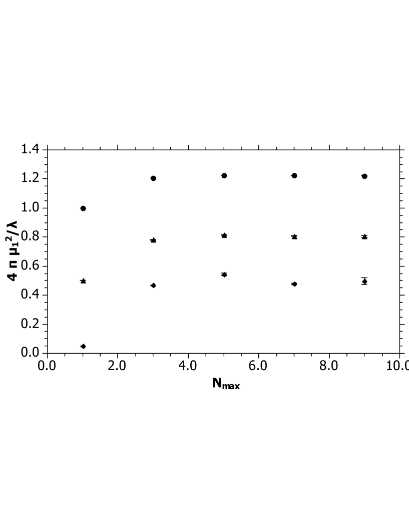
Figure 4: Plot of the scaled bare mass $\tilde{\mu}_{1}^{2}=4\pi\mu_{1}^{2}/\lambda$ versus the Fock-space truncation at $N_{\rm max}$ constituents, for three values of $\tilde{M}^{2}$: 1.0 (circles), 0.5 (triangles), and 0.05 (diamonds). The error bars represent uncertainties in extrapolations.

References

- (1) M. Burkardt, S.S. Chabysheva, and J.R. Hiller, Phys. Rev. D 94, 065006 (2016).
- (2) S.-J. Chang, Phys. Rev. D 12, 1071 (1975); 13, 2778 (1976).
- (3) S. Rychkov and L.G. Vitale, Phys. Rev. D 91, 085011 (2015).
- (4) D. Lee and N. Salwen, Phys. Lett. B 503, 223 (2001).
- (5) T. Sugihara, J. High Energy Phys. 05(2004), 007 (2004).
- (6) D. Schaich and W. Loinaz, Phys. Rev. D 79, 056008 (2009).
- (7) P. Bosetti, B. De Palma, and M. Guagnelli, Phys. Rev. D 92, 034509 (2015).
- (8) A. Milsted, J. Haegeman, and T.J. Osborne, Phys. Rev. D 88, 085030 (2013).
- (9) A. Harindranath and J.P. Vary, Phys. Rev. D 36, 1141 (1987).
- (10) M. Burkardt, Phys. Rev. D 47, 4628 (1993).
- (11) R.J. Perry, A. Harindranath, and K.G. Wilson, Phys. Rev. Lett. 65, 2959 (1990); R.J. Perry and A. Harindranath, Phys. Rev. D 43, 4051 (1991).
- (12) J.R. Hiller and S.J. Brodsky, Phys. Rev. D 59, 016006 (1998).
- (13) V.A. Karmanov, J.-F. Mathiot, and A.V. Smirnov, Phys. Rev. D 77, 085028 (2008); Phys. Rev. D 82, 056010 (2010).
- (14) S.S. Chabysheva and J.R. Hiller, Ann. Phys. 325, 2435 (2010).
- (15) B. Elliott, S.S. Chabysheva, and J.R. Hiller, Phys. Rev. D 90, 056003 (2014).
- (16) J.R. Hiller, Prog. Part. Nucl. Phys. 90, 75 (2016); M. Burkardt, Adv. Nucl. Phys. 23, 1 (2002); S.J. Brodsky, H.-C. Pauli, and S.S. Pinsky, Phys. Rep. 301, 299 (1998).
- (17) P.A.M. Dirac, Rev. Mod. Phys. 21, 392 (1949).
- (18) S.S. Chabysheva and J.R. Hiller, Phys. Rev. E 90, 063310 (2014); S.S. Chabysheva, B. Elliott and J.R. Hiller, Phys. Rev. E 88, 063307 (2013).
- (19) K.G. Wilson, Nucl. Proc. B (Proc. Suppl.) 17, 82 (1990).
- (20) S.S. Chabysheva and J.R. Hiller, Phys. Lett. B 711, 417 (2012).