Abstract

We study the one-loop electroweak radiative corrections to $h^{0}\to b\bar{b}$ and $h^{0}\to\tau^{+}\tau^{-}$ in the framework of two Higgs doublet Model (2HDM). We evaluate the deviation of these couplings from their Standard Model (SM) values. $h^{0}\to b\bar{b}$ and $h^{0}\to\tau^{+}\tau^{-}$ may receives large contribution from triple Higgs couplings $h^{0}H^{0}H^{0}$, $H^{0}h^{0}h^{0}$, $h^{0}A^{0}A^{0}$ and $h^{0}H^{+}H^{-}$ which are absent in the Standard Model. It is found that in 2HDM, these corrections could be significant and may reach more than 12% for not tow heavy $H^{0}$ or $A^{0}$ or $H^{\pm}$. We also study the ratio of branching ratios $R=BR(h^{0}\to b\bar{b})/BR(h^{0}\to\tau^{+}\tau^{-})$ of Higgs boson decays which could be used to disentangle SM from other models such as 2HDM.

1 Introduction

A Higgs-like particle has been discovered in the first run of the LHC with 7 and 8 TeV energy in 2012 [2, 1]. The combined measured Higgs boson mass obtained by the ATLAS and CMS collaborations based on the data from 7 and 8 TeV is $m_{h}=$ 125.09 $\pm$ 0.21 (stat.) $\pm$ 0.11 (syst.) GeV [3]. ATLAS and CMS also performed several Higgs coupling measurements, such as Higgs couplings to $W^{+}W^{-}$, $ZZ$, $\gamma\gamma$, $b\bar{b}$ and $\tau^{+}\tau^{-}$ with 20-30% uncertainty, while the coupling to $b\bar{b}$ still suffers from a large uncertainty of $40-50$%. One of the tasks of the new LHC run at 13 TeV (and 14 TeV) would be to improve all the aforementioned measurements and to perform new ones such as accessing $h^{0}\to\gamma Z$ as well as the triple self-coupling of the Higgs boson. It is expected that the new LHC run will pin down the uncertainty in $h^{0}\to b\bar{b}$ and $h^{0}\to\tau^{+}\tau^{-}$ to $10$-$13\%$ and $6$-$8\%$ for bottom quarks and tau leptons, respectively. These measurements will be further ameliorated by the High Luminosity option for the LHC (HL-LHC) down to uncertainties of $4$-$7\%$ for $b$ quarks and $2$-$5\%$ for $\tau$ leptons [4]. Moreover, in the clean environment of the $e^{+}e^{-}$ Linear Collider (LC), which can act as a Higgs factory, the uncertainties on $h\to b\bar{b}$ and $h^{0}\to\tau^{+}\tau^{-}$ would be much smaller reaching $0.6\%$ for the couplings in $h^{0}\to b\bar{b}$ and $1.3\%$ for those in $h^{0}\to\tau^{+}\tau^{-}$ [5, 6].

The above accuracies on fermionic Higgs decay measurements, if reached, are of the size comparable to the effects of radiative corrections to some Higgs decays. Therefore, one can use these radiative correction effects to distinguish between the Standard Model (SM) and various beyond-standard models. In this respect, precise calculations of Higgs-boson production and decay rates have been performed already quite some time ago with great achievements (see e.g. [7, 21]). QCD corrections to Higgs decays into quarks are very well known up to ${\cal O}(\alpha_{s}^{3})$ as well as additional corrections at ${\cal O}(\alpha_{s}^{2})$ that involve logarithms of the light-quark masses and also heavy top contributions [7]. Electroweak radiative corrections to fermionic decays ($b\bar{b}$ and $\tau^{+}\tau^{-}$) of the Higgs boson in the SM are also well established [10, 9, 11] in the on-shell scheme. In the framework of the Two-Higgs-Doublet Model (2HDM), several studies have been carried out to evaluate the electroweak corrections to fermionic Higgs decays [12, 13]. The calculation of Ref. [12] is done in the on-shell scheme except for the Higgs field renormalization where the $\overline{MS}$ subtraction has been used, while the one of Ref. [13] is performed using the on-shell renormalization scheme of [15].

In this paper, we will study the effects of electroweak radiative corrections to $h^{0}\to b\bar{b}$ and $h^{0}\to\tau^{+}\tau^{-}$ decays in the 2HDM taking into account theoretical constraints as well as experimental restrictions from recent LHC data and other experimental results. For $h^{0}\to b\bar{b}$ we will update our results from [12] while for $h^{0}\to\tau^{+}\tau^{-}$ we will compute these effects for the first time following the same renormalization procedure described in [12]. Similar studies have been performed in [16, 17] to which we will compare our results. We will also use our calculations to evaluate the ratio of branching fractions of Higgs decays in the 2HDM  [18, 19],

$$R=\frac{BR(h^{0}\to b\bar{b})}{BR(h^{0}\to\tau^{+}\tau^{-})}.$$ (1)

Such a ratio of Higgs boson decay widths is independent of the production process and therefore is insensitive to higher-order QCD corrections and also to new physics effects that may affect the production rate of the Higgs. This ratio has also the particularity of being less sensitive to the systematic errors (which drop out in the ratio) and could be used to discriminate the SM against other models such as 2HDM or supersymmetric models.

The paper is organized as follows. In Section 2 we review the Yukawa textures, scalar potential and Higgs self-couplings of the 2HDM model, as well as the theoretical and experimental constraints on the model. Section 3 outlines the calculation and specifies the renormalization scheme we will be using. The numerical results are presented in Section 6. Finally, we conclude in Section 6.

2 The 2HDM model

2.1 Yukawa textures

In the 2HDM, fermion and gauge boson masses are generated from two Higgs doublets $\Phi_{1,2}$ where both of them acquire vacuum expectation values $v_{1,2}$. If both Higgs fields couple to all fermions, Flavor Changing Neutral Currents (FCNC) are generated which can invalidate some low energy observables in B, D and K physics. In order to avoid such FCNC, the Paschos-Glashow-Weinberg theorem [20] proposes a $Z_{2}$ symmetry that forbids FCNC couplings at the tree level. Depending on the $Z_{2}$ assignment, we have four type of models [22, 21]. In the 2HDM type-I model, only the second doublet $\Phi_{2}$ interacts with all the fermions like in SM. In 2HDM type-II model the doublet $\Phi_{2}$ interacts with up-type quarks and $\Phi_{1}$ interacts with the down-type quarks and charged leptons. In 2HDM type-III, charged leptons couple to $\Phi_{1}$ while all the quarks couple to $\Phi_{2}$. Finally, in 2HDM type IV, charged leptons and up-type quarks couple to $\Phi_{2}$ while down-type quarks acquire masses from their couplings to $\Phi_{1}$.

The most general Yukawa interactions can be written as follows,

$$-{\mathcal{L}}_{\text{Yukawa}}^{\text{2HDM}}= {\overline{Q}}_{L}Y_{u}\widetilde{\Phi}_{2}u_{R}+{\overline{Q}}_{L}Y_{d}\Phi_{d}d_{R}+{\overline{L}}_{L}Y_{\ell}\Phi_{\ell}\ell_{R}+\text{h.c},$$ (2)

where $\Phi_{d,l}$ ($d,l=1,2$) represents $\Phi_{1}$ or $\Phi_{2}$ and $Y_{f}$ ($f=u,d$ or $\ell$) stands for Yukawa matrices. The two complex scalar $SU(2)$ doublets can be decomposed according to

$$\Phi_{i}=\left(\begin{array}[]{c}\phi_{i}^{+}\\ \left(v_{i}+\rho_{i}+i\eta_{i}\right)\left/\sqrt{2}\right.\end{array}\right),\quad i=1,2,$$ (5)

where $v_{1,2}$ are the vacuum expectation values of $\Phi_{1,2}$. The mass eigenstates for the Higgs bosons are obtained by orthogonal transformations,

$$\left(\begin{array}[]{c}\phi_{1}^{\pm}\\ \phi_{2}^{\pm}\end{array}\right) =R_{\beta}\left(\begin{array}[]{c}G^{\pm}\\ H^{\pm}\end{array}\right),\quad\left(\begin{array}[]{c}\rho_{1}\\ \rho_{2}\end{array}\right)=R_{\alpha}\left(\begin{array}[]{c}H^{0}\\ h^{0}\end{array}\right),\quad\left(\begin{array}[]{c}\eta_{1}\\ \eta_{2}\end{array}\right)=R_{\beta}\left(\begin{array}[]{c}G^{0}\\ A^{0}\end{array}\right),$$ (18)

with the generic orthogonal matrix

$$R_{\theta}=\left(\begin{array}[]{cc}\cos\theta&-\sin\theta\\ \sin\theta&\cos\theta\end{array}\right).$$

type	$\xi_{u}^{h^{0}}$	$\xi_{d}^{h^{0}}$	$\xi_{l}^{h^{0}}$	$\xi_{u}^{H^{0}}$	$\xi_{d}^{H^{0}}$	$\xi_{l}^{H^{0}}$	$\xi_{u}^{A^{0}}$	$\xi_{d}^{A^{0}}$	$\xi_{l}^{A^{0}}$
I	$c_{\alpha}/s_{\beta}$	$c_{\alpha}/s_{\beta}$	$c_{\alpha}/s_{\beta}$	$s_{\alpha}/s_{\beta}$	$s_{\alpha}/s_{\beta}$	$s_{\alpha}/s_{\beta}$	$\cot\beta$	$-\cot\beta$	$-\cot\beta$
II	$c_{\alpha}/s_{\beta}$	$-s_{\alpha}/c_{\beta}$	$-s_{\alpha}/c_{\beta}$	$s_{\alpha}/s_{\beta}$	$c_{\alpha}/c_{\beta}$	$c_{\alpha}/c_{\beta}$	$\cot\beta$	$\tan\beta$	$\tan\beta$
III	$c_{\alpha}/s_{\beta}$	$c_{\alpha}/s_{\beta}$	$-s_{\alpha}/c_{\beta}$	$s_{\alpha}/s_{\beta}$	$s_{\alpha}/s_{\beta}$	$c_{\alpha}/c_{\beta}$	$\cot\beta$	$-\cot\beta$	$\tan\beta$
IV	$c_{\alpha}/s_{\beta}$	$-s_{\alpha}/c_{\beta}$	$c_{\alpha}/s_{\beta}$	$s_{\alpha}/s_{\beta}$	$c_{\alpha}/c_{\beta}$	$s_{\alpha}/s_{\beta}$	$\cot\beta$	$\tan\beta$	$-\cot\beta$

Table 1: Yukawa coupling coefficients of the neutral Higgs bosons $h^{0},H^{0},A^{0}$ to the up-quarks, down-quarks and the charged leptons ($u,d,\ell$) in the four 2HDM types.

From the eight fields initially present in the two scalar doublets, three of them, namely the Goldstone bosons $G^{\pm}$ and $G^{0}$, are eaten by the longitudinal components of $W^{\pm}$ and $Z$, respectively. The remaining five are physical Higgs fields, two CP-even $H^{0}$ and $h^{0}$, a CP-odd $A^{0}$, and a pair of charged scalars $H^{\pm}$.

Writing the Yukawa interactions eq. (2) in terms of mass eigenstates of the neutral and charged Higgs bosons yields

$$-{\mathcal{L}}_{\text{Yukawa}}^{\text{2HDM}} = \sum_{f=u,d,\ell}\frac{m_{f}}{v}\left(\xi_{f}^{h^{0}}{\overline{f}}fh^{0}+\xi_{f}^{H^{0}}{\overline{f}}fH^{0}-i\xi_{f}^{A^{0}}{\overline{f}}\gamma_{5}fA^{0}\right)$$

$$+\left\{\frac{\sqrt{2}V_{ud}}{v}\,\overline{u}\left(m_{u}\xi_{u}^{A^{0}}\text{P}_{L}+m_{d}\xi_{d}^{A^{0}}\text{P}_{R}\right)dH^{+}+\frac{\sqrt{2}m_{\ell}\xi_{\ell}^{A^{0}}}{v}\,\overline{\nu_{L}}\ell_{R}H^{+}+\text{h.c}\right\},$$

where $v^{2}=v_{1}^{2}+v_{2}^{2}=(\sqrt{2}G_{F})^{-1}$; $P_{R}$ and $P_{L}$ are the right- and left-handed projection operators, respectively. The coefficients $\xi^{h^{0}}_{f},\xi^{H^{0}}_{f}$ and $\xi^{A^{0}}_{f}$ ($f=u,d,l$) in the four 2HDM types are given in the Table 1.

2.2 Scalar potential and self-coupling of the Higgs bosons

The most general 2HDM scalar potential which is invariant under $SU(2)_{L}\otimes U(1)_{Y}$ and possesses a soft $Z_{2}$ breaking term ($m_{12}^{2}$) [21, 22, 23] can be written in the following way,

$${V}_{\rm 2HDM} = m_{11}^{2}\Phi_{1}^{\dagger}\Phi_{1}+m_{22}^{2}\Phi_{2}^{\dagger}\Phi_{2}-m_{12}^{2}\left(\Phi_{1}^{\dagger}\Phi_{2}+\Phi_{2}^{\dagger}\Phi_{1}\right)+\frac{\lambda_{1}}{2}(\Phi_{1}^{\dagger}\Phi_{1})^{2}+\frac{\lambda_{2}}{2}(\Phi_{2}^{\dagger}\Phi_{2})^{2}$$ (20)

$$+\lambda_{3}(\Phi_{1}^{\dagger}\Phi_{1})(\Phi_{2}^{\dagger}\Phi_{2})+\lambda_{4}\left|\Phi_{1}^{\dagger}\Phi_{2}\right|^{2}+\frac{\lambda_{5}}{2}\left\{\left(\Phi_{1}^{\dagger}\Phi_{2}\right)^{2}+\left(\Phi_{2}^{\dagger}\Phi_{1}\right)^{2}\right\}.$$

Hermiticity of the potential requires $m_{11}^{2}$, $m_{22}^{2}$ and $\lambda_{1,2,3,4}$ to be real, while $m_{12}^{2}$ and $\lambda_{5}$ could be complex in case one would allow for CP violation in the Higgs sector. In what follows we assume that there is no CP violation, which means $m_{12}^{2}$ and $\lambda_{5}$ are taken as real.

From the above potential, Eq. (20), we can derive the triple Higgs couplings, needed for the present study as a function of the 2HDM parameters $m_{h^{0}}$, $m_{H^{0}}$, $m_{A^{0}}$, $m_{H^{\pm}}$, $\tan\beta$, $\alpha$ and $m_{12}^{2}$. These couplings follow from the scalar potential and are thus independent of the Yukawa types used; they are given by

$$\lambda_{h^{0}h^{0}h^{0}}^{2HDM} = \frac{-3g}{2m_{W}s^{2}_{2\beta}}\bigg{[}(2c_{\alpha+\beta}+s_{2\alpha}s_{\beta-\alpha})s_{2\beta}m^{2}_{h^{0}}-4c^{2}_{\beta-\alpha}c_{\beta+\alpha}m^{2}_{12}\bigg{]}$$

$$\lambda_{H^{0}h^{0}h^{0}}^{2HDM} = -\frac{1}{2}\frac{gc_{\beta-\alpha}}{m_{W}s^{2}_{2\beta}}\bigg{[}(2m^{2}_{h}+m^{2}_{H^{0}})s_{2\alpha}s_{2\beta}-2(3s_{2\alpha}-s_{2\beta})m^{2}_{12}\bigg{]}$$

$$\lambda_{h^{0}H^{0}H^{0}}^{2HDM} = \frac{1}{2}\frac{gs_{\beta-\alpha}}{m_{W}s^{2}_{2\beta}}\bigg{[}(m^{2}_{h^{0}}+2m^{2}_{H^{0}})s_{2\alpha}s_{2\beta}-2(3s_{2\alpha}+s_{2\beta})m^{2}_{12}\bigg{]}$$

$$\lambda_{h^{0}H^{\pm}H^{\mp}}^{2HDM} = \frac{1}{2}\frac{g}{m_{W}}\bigg{[}(m^{2}_{h^{0}}-2m^{2}_{H^{\pm}})s_{\beta-\alpha}-\frac{2c_{\beta+\alpha}}{s^{2}_{2\beta}}(m^{2}_{h}s_{2\beta}-2m^{2}_{12})\bigg{]}$$

$$\lambda_{h^{0}A^{0}A^{0}}^{2HDM} = \frac{1}{2}\frac{g}{m_{W}}\bigg{[}(m^{2}_{h}-2m^{2}_{A^{0}})s_{\beta-\alpha}-\frac{2c_{\beta+\alpha}}{s^{2}_{2\beta}}(m^{2}_{h}s_{2\beta}-2m^{2}_{12})\bigg{]},$$ (21)

with the $W$ boson mass $m_{W}$ and the $SU(2)$ gauge coupling constant $g$. We have used the notation $s_{x}$ and $c_{x}$ as short-hand notations for $\sin(x)$ and $\cos(x)$, respectively. The mixing angle $\beta$ is defined by via $\tan\beta=v_{2}/v_{1}$, where $v_{i}$ are the vacuum expectation values of the Higgs fields $\Phi_{i}$.

It has been shown that the 2HDM has a decoupling limit which is reached for $\cos(\beta-\alpha)=0$ and $m_{H^{0},A^{0},H^{\pm}}\gg m_{Z}$ [23]. In this limit, the coupling of the CP-even $h^{0}$ to SM particles completely mimic the SM Higgs couplings including the triple coupling $h^{0}h^{0}h^{0}$. Moreover, the model possesses also an alignment limit [24], in which one of the CP-even Higgs bosons $h^{0}$ or $H^{0}$ looks like SM Higgs particle if $\sin(\beta-\alpha)\to 1$ or $\cos(\beta-\alpha)\to 1$.
In the limit $\alpha=\beta-\pi/2$ (which will be used for our numerical analysis) the above triple Higgs couplings reduce to the simplified form

$$\lambda_{h^{0}h^{0}h^{0}}^{2HDM} = \frac{-3g}{2m_{W}}m^{2}_{h^{0}}=\lambda_{hhh}^{SM},$$

$$\lambda_{H^{0}h^{0}h^{0}}^{2HDM} = 0,$$

$$\lambda_{h^{0}H^{0}H^{0}}^{2HDM} = \frac{g}{m_{W}}\bigg{[}\bigg{(}\frac{2m^{2}_{12}}{s_{2\beta}}-m^{2}_{H^{0}}\bigg{)}-\frac{m^{2}_{h^{0}}}{2}\bigg{]},$$

$$\lambda_{h^{0}H^{\pm}H^{\mp}}^{2HDM} = \frac{g}{m_{W}}\bigg{[}\bigg{(}\frac{2m^{2}_{12}}{s_{2\beta}}-m^{2}_{H^{\pm}}\bigg{)}-\frac{m^{2}_{h^{0}}}{2}\bigg{]},$$

$$\lambda_{h^{0}A^{0}A^{0}}^{2HDM} = \frac{g}{m_{W}}\bigg{[}\bigg{(}\frac{2m^{2}_{12}}{s_{2\beta}}-m^{2}_{A^{0}}\bigg{)}-\frac{m^{2}_{h^{0}}}{2}\bigg{]},$$ (22)

where we can see that in the degenerate case, $m_{H^{\pm}}=m_{H^{0}}=m_{A^{0}}=m_{S}$, all triple Higgs couplings $h^{0}H^{0}H^{0}$, $h^{0}A^{0}A^{0}$ and $h^{0}H^{\pm}H^{\mp}$ have the same expression, labeled by $h^{0}SS$,

$$\lambda_{h^{0}SS}^{2HDM} = \frac{g}{m_{W}}\bigg{[}\bigg{(}\frac{2m^{2}_{12}}{s_{2\beta}}-m^{2}_{S^{0}}\bigg{)}-\frac{m^{2}_{h^{0}}}{2}\bigg{]}.$$ (23)

2.3 Theoretical and experimental constraints

The 2HDM has several theoretical constraints which we briefly address here. In order to ensure vacuum stability of the 2HDM, the scalar potential must satisfy conditions that guarantee that its bounded from below, i.e. that the requirement ${V}_{\rm 2HDM}\geq 0$ is satisfied for all directions of $\Phi_{1}$ and $\Phi_{2}$ components. This requirement imposes the following conditions on the coefficients $\lambda_{i}$ [25, 26]:

$$\lambda_{1}>0\quad,\quad\lambda_{2}>0\quad,\quad\lambda_{3}+2\sqrt{\lambda_{1}\lambda_{2}}>0\quad\quad,\quad\quad\lambda_{3}+\lambda_{4}-|\lambda_{5}|>2\sqrt{\lambda_{1}\lambda_{2}}.$$ (24)

In addition to the constraints from positivity of the scalar potential, there is another set of constraints by requiring perturbative tree-level unitarity for scattering of Higgs bosons and longitudinally polarized gauge bosons. These constraints are taken from [28, 27]. Moreover, we also force the potential to be perturbative by imposing that all quartic coefficients of the scalar potential satisfy $|\lambda_{i}|\leq 8\pi$ ($i=1,...,5$).

Besides these theoretical bounds, we have indirect experimental constraints from $B$ physics observables on 2HDM parameters such as $\tan\beta$ and the charged Higgs boson mass. It is well known that in the framework of 2HDM-II and IV, for example, the measurement of the $b\to s\gamma$ branching ratio requires the charged Higgs boson mass to be heavier than 580 GeV [29, 30] for any value of $\tan\beta\geq 1$. Such a limit is much lower for the other 2HDM types [31]. In 2HDM-I and III, as long as $\tan\beta\geq 2$, it is possible to have charged Higgs bosons as light as 100 GeV [31, 32] while being consistent with all $B$ physics constraints as well as with LEP and LHC limits [33, 34, 35, 36, 37, 38].
We stress in passing that after the Higgs-like particle discovery, several theoretical studies have performed global-fit analyses for the 2HDM to pin down the allowed regions of parameter space both for a SM-like Higgs $h^{0}$ [39] as well as for a SM-like Higgs boson $H^{0}$ [40].

Table 2: Combined best-fit signal strengths $\widehat{\mu}_{\rm{1}}$ and $\widehat{\mu}_{\rm{2}}$ and the associated correlation coefficient $\rho$ for corresponding Higgs decay mode [41].

$f$	$\widehat{\mu}^{f}_{\rm{1}}$	$\widehat{\mu}^{f}_{\rm{2}}$	$\pm\,\,1\widehat{\sigma}_{\rm{1}}$	$\pm\,\,1\widehat{\sigma}_{\rm{2}}$
$\gamma\gamma$	$1.16$	0.18	0.16	0.7
$ZZ^{*}$	$1.70$	0.3	0.4	1.20
$WW^{*}$	$0.98$	1.28	0.28	0.55
$\tau^{+}\tau^{-}$	$2$	1.24	1.50	0.59
$b\bar{b}$	1.11	0.92	0.65	0.38

Moreover, we take into account experimental data from the observed cross section times branching ratio divided by SM predictions for the various channels, i.e. the signal strengths of the Higgs boson defined by

$$\mu^{f}_{i} = \frac{\sigma(i\rightarrow h^{0})^{2HDM}Br(h^{0}\rightarrow f)^{2HDM}}{\sigma(i\rightarrow h^{0})^{SM}Br(h^{0}\rightarrow f)^{SM}},\quad\quad\quad i=1,2$$ (25)

where $\sigma(i\rightarrow h^{0})$ denotes the Higgs-boson production cross section through channel $i$ and $Br(h^{0}\rightarrow f)$ is the branching ratio for the Higgs decay $h^{0}\rightarrow f\bar{f}$. Since several Higgs production channels are available at the LHC, they are grouped to be $\mu^{f}_{1}=\mu^{f}_{ggF+tth^{0}}$ and $\mu^{f}_{2}=\mu^{f}_{VBF+Vh^{0}}$, containing gluon fusion (ggF) plus associated Higgs production $t\bar{t}h^{0}$, and vector boson fusion (VBF) plus Higgs-strahlung $Vh^{0}$ with $V=Z/W$. We summarize relevant signal strengths associated to each Higgs production and decay channels in Table 2 with the overall combinations obtained by the ATLAS and CMS collaborations.

3 One-loop calculation and renormalization scheme

Calculations of higher order corrections in perturbation theory in general lead to ultra-violet (UV) divergences. The standard procedure to eliminate these UV divergences consists in renormalization of the bare Lagrangian by redefinition of couplings and fields. In the SM, the on-shell renormalization scheme is well elaborated [42, 43, 44]. For the 2HDM, several extensions of the SM renormalization scheme exist in the literature [13, 15, 12, 45]. Recently, gauge independent renormalization schemes have been proposed [47, 46], with e.g. $\overline{\rm{MS}}$ renormalization for the mixing angles and the soft $Z_{2}$ breaking term in the Higgs sector [47]. In the present study, we adopt the on-shell renormalization scheme used also in [12], which is an extension of the on-shell scheme of the SM: the gauge sector is renormalized in analogy to [42, 43] concerning vector-boson masses and field renormalization; also fermion mass and field renormalization is treated in an analogous way (see also [44]). For renormalization of the Higgs sector we take over the approach used in [12], which means on-shell renormalization

• for the $h^{0},H^{0}$ tadpoles, yielding zero for the renormalized tadpoles and thus $v_{1,2}$ at the minimum of the potential also at one-loop order,

• for all physical masses from the Higgs potential, defining the masses $m_{h^{0}},m_{H^{0}},m_{A^{0}},m_{H^{\pm}}$ as pole masses,

whereas Higgs field renormalization is done in the ${\overline{\rm MS}}$ scheme. We assign renormalization constants $Z_{\Phi_{i}}$ for the two Higgs doublets in (5) and counter-terms for the $v_{i}$ within the doublets, according to

$$\Phi_{i}\rightarrow(Z_{\Phi_{i}})^{1/2}\Phi_{i}\qquad,\qquad v_{i}\rightarrow v_{i}-\delta v_{i}\,,$$ (26)

and expand the $Z$ factors $Z_{\Phi_{i}}=1+\delta Z_{\Phi_{i}}$ to one-loop order. The $\overline{\rm{MS}}$ condition yields the field renormalization constants as follows for all types of models listed in Table 1:

$$\delta Z_{\Phi_{1}}^{\overline{\rm MS}} = \frac{\Delta}{32\pi^{2}}\biggl{\{}\frac{-g^{2}}{m_{W}^{2}t_{\beta}}\biggl{(}\xi_{l}^{A^{0}}\biggl{[}m_{e}^{2}+m_{\mu}^{2}+m_{\tau}^{2}\biggr{]}(1+t_{\beta}\xi_{l}^{A})+N_{C}\xi_{d}^{A^{0}}\biggl{[}m_{b}^{2}+m_{d}^{2}+m_{s}^{2}\biggr{]}(1+t_{\beta}\xi_{d}^{A^{0}})$$

$$-N_{C}\xi_{u}^{A^{0}}\biggl{[}m_{c}^{2}+m_{t}^{2}+m_{u}^{2}\biggr{]}(1-t_{\beta}\xi_{u}^{A^{0}})\biggr{)}+(3g^{2}+g^{\prime 2})\biggr{\}}\,,$$

$$\delta Z_{\Phi_{2}}^{\overline{\rm MS}} = \frac{\Delta}{32\pi^{2}}\biggl{\{}\frac{-g^{2}}{m_{W}^{2}}\biggl{(}-\xi_{l}^{A^{0}}\biggl{[}m_{e}^{2}+m_{\mu}^{2}+m_{\tau}^{2}\biggr{]}(t_{\beta}-\xi_{l}^{A^{0}})-N_{C}\xi_{d}^{A^{0}}\biggl{[}m_{b}^{2}+m_{d}^{2}+m_{s}^{2}\biggr{]}(t_{\beta}-\xi_{d}^{A^{0}})$$ (27)

$$+N_{C}\xi_{u}^{A^{0}}\biggl{[}m_{c}^{2}+m_{t}^{2}+m_{u}^{2}\biggr{]}(t_{\beta}+\xi_{u}^{A^{0}})\biggr{)}+(3g^{2}+g^{\prime 2})\biggr{\}}\,,$$

with $\Delta=2/(4-D)-\gamma+{\rm log}4\pi$ from dimensional regularization, the color factor $N_{C}=3$ for quarks and $N_{C}=1$ for leptons, and the gauge couplings $g$ and $g^{\prime}$. The factors $\xi_{u,d,l}^{A^{0}}$ can be found in Table 1. Eq. (3) is a generalization of the work of [12] with respect to the various Yukawa structures of the 2HDM.

The renormalized self-energy of the SM-like Higgs field $h^{0}$ is the following finite combination of the unrenormalized self-energy and counter-terms,

$$\widehat{\Sigma}_{h^{0}}(k^{2})={\Sigma}_{h^{0}}(k^{2})-\delta m^{2}_{h^{0}}+(k^{2}-m^{2}_{h^{0}})\,\delta Z_{h^{0}}$$ (28)

with the on-shell mass counter-term $\delta m^{2}_{h^{0}}$ and $\delta Z_{h^{0}}=s_{\alpha}^{2}\delta Z^{\overline{\rm MS}}_{\Phi_{1}}+c_{\alpha}^{2}\delta Z^{\overline{\rm MS}}_{\Phi_{2}}$.

Owing to the $\overline{\rm{MS}}$ field renormalization, a finite wave function renormalization has to be assigned to each external $h^{0}$ in a physical amplitude. This quantity is determined by the derivative of the renormalized self-energy $\widehat{\Sigma}_{h^{0}}^{\prime}$ on the mass shell, given by

$$\widehat{\Sigma}_{h^{0}}^{\prime}(m_{h^{0}}^{2})=\Sigma_{h^{0}}^{\prime}(m_{h^{0}}^{2})+(s_{\alpha}^{2}\delta Z_{\Phi_{1}}^{\overline{\rm MS}}+c_{\alpha}^{2}\delta Z_{\Phi_{2}}^{\overline{\rm MS}}).\,$$ (29)

Application to the one-loop calculation for the fermionic Higgs boson decay $h^{0}\rightarrow f\bar{f}$ yields the decay amplitude which can be written as follows,

$${\cal M}_{1}=-\frac{igm_{f}}{2m_{W}}\sqrt{\widehat{Z}_{h^{0}}}\left[\xi_{f}^{h^{0}}(1+\Delta{\cal M}_{1})+\xi_{f}^{H^{0}}\Delta{\cal M}_{12}\right]$$ (30)

where

$$\Delta{\cal M}_{1} = V_{1}^{h^{0}f\bar{f}}+\delta(h^{0}f\bar{f}),$$ (31)

$$\Delta{\cal M}_{12} = \frac{\Sigma_{h^{0}H^{0}}(m_{h^{0}}^{2})}{m_{h^{0}}^{2}-m_{H^{0}}^{2}}-\delta\alpha\,,$$ (32)

$$\widehat{Z}_{h^{0}} = \left[1+\widehat{\Sigma}_{h^{0}}^{\prime}(m_{h^{0}}^{2})\right]^{-1}\,.$$ (33)

$\Delta{\cal M}_{1}$ is the sum of the one-loop vertex diagrams $V_{1}^{h^{0}f\bar{f}}$ and the vertex counter-term $\delta(h^{0}f\bar{f})$, $\Sigma_{h^{0}H^{0}}$ is the $h^{0}$–$H^{0}$ mixing, $\delta\alpha$ represents the counter-term for the mixing angle $\alpha$, and $\hat{Z}_{h^{0}}$ is the finite wave function renormalization of the external $h^{0}$ fixed by the derivative of the renormalized self-energy specified above in (29). Given the fact that the mixing angle $\alpha$ is an independent parameter, it can be renormalized in a way independent of all the other renormalization conditions. A simple renormalization condition for $\alpha$ is to require that $\delta\alpha$ absorbs the transition $h^{0}$-$H^{0}$ in the non-diagonal part $\Delta{\cal M}_{12}$ of the fermionic Higgs decay amplitude. Therefore, the angle $\alpha$ is hence the CP-even Higgs-boson mixing angle also at the one-loop level, and the decay amplitude ${\cal M}_{1}$ simplifies to the $\Delta{\cal M}_{1}$ term only.

The amplitude (30) together with its ingredients is a generalization of the work in  [12], extended to all charged fermions and for the various 2HDM types. $\Delta{\cal M}_{1}$ contains besides the genuine vertex corrections the counter-term $\delta(h^{0}f\bar{f})$ for Higgs-fermion-fermion vertex, which reads as follows,

$$\delta(h^{0}f\bar{f})=\frac{\delta m_{f}}{m_{f}}+\delta Z_{V}^{f}+\frac{\delta v}{v}\,,$$ (34)

where

$$\frac{\delta m_{f}}{m_{f}}+\delta Z_{V}^{f}=\Sigma_{S}^{f}(m_{f}^{2})-2m_{f}^{2}\left[\Sigma_{S}^{\prime b}(m_{f}^{2})+\Sigma_{V}^{\prime f}(m_{f}^{2})\right]$$ (35)

can be expressed in terms of the scalar functions of the fermion self-energy,

$$\Sigma^{f}(p) = \not{\!p}\,\Sigma_{V}^{f}(p^{2})\,+\,\not{\!p}\gamma_{5}\,\Sigma_{A}^{f}(p^{2})\,+\,m_{f}\,\Sigma_{S}^{f}(p^{2})\,,$$ (36)

and the universal part

$$2\frac{\delta v}{v}=2\frac{\delta v_{1,2}}{v_{1,2}} = c_{\beta}^{2}\,\delta Z_{\Phi_{1}}^{\overline{\rm MS}}+s_{\beta}^{2}\,\delta Z_{\Phi_{2}}^{\overline{\rm MS}}$$

$$+ \Sigma_{\gamma\gamma}^{\prime}(0)+2\frac{s_{W}}{c_{W}}\frac{\Sigma_{\gamma Z}(0)}{m_{Z}^{2}}-\frac{c_{W}^{2}}{s_{W}^{2}}\frac{\Re\Sigma_{ZZ}(m_{Z}^{2})}{m_{Z}^{2}}+\frac{c_{W}^{2}-s_{W}^{2}}{s_{W}^{2}}\frac{\Re\Sigma_{WW}(m_{W}^{2})}{m_{W}^{2}}\,.$$

This universality is a consequence of the renormalization condition

$$\frac{\delta v_{1}}{v_{1}}-\frac{\delta v_{2}}{v_{2}} = 0$$ (38)

(see the discussion in [12]), which is also used in the Minimal Supersymmetric SM (MSSM), see e.g. [50, 51, 52]. It is important that the singular part of the difference in the lhs. of (38) vanishes. The singular part of $\delta v$ is $(\delta v/v)_{\overline{\rm MS}}=-\frac{1}{64\pi^{2}}(3g^{2}+g^{\prime 2})\Delta$, which is equal to the expression found in the MSSM and constitutes a check of our calculation.

We end this section by showing in Fig. (1) the one-loop Feynman diagrams in 2HDM for $h^{0}\rightarrow b\overline{b}$ and $h^{0}\rightarrow\tau^{+}\tau^{-}$, where S stands for ($H^{\pm},A^{0},H^{0},G^{\pm})$ for both decays while F represents ($b$,$t$) for $h^{0}\rightarrow b\overline{b}$ and ($\tau,\nu_{\tau}$) for $h^{0}\rightarrow\tau^{+}\tau^{-}$. In the SM limit [23], diagrams (4, 5, 10, 11) and (2, 8) with (S,S)=($H^{\pm},G^{\pm})$ vanish. Consequently, the important effects come from diagrams (1, 2) and (7,8) respectively for $h^{0}\rightarrow b\overline{b}$ and $h^{0}\rightarrow\tau^{+}\tau^{-}$.

In the present work, computation of all the one-loop amplitudes and counter-terms is done with the help of FeynArts and FormCalc [53] packages. Numerical evaluations of the scalar integrals are done with LoopTools [54]. We have also tested the cancellation of UV divergences both analytically and numerically.

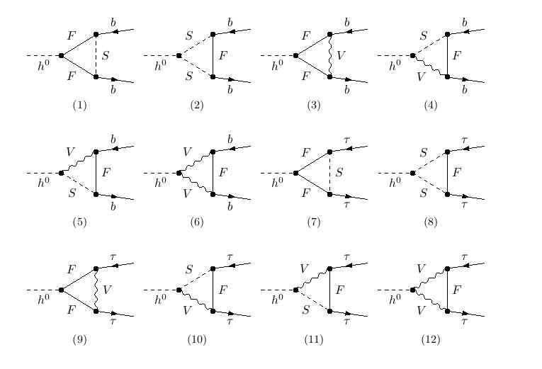
Figure 1: Generic one-loop 2HDM Feynman diagrams contributing to $\Gamma_{1}(h^{0}\rightarrow b\overline{b})$ and $\Gamma_{1}(h^{0}\rightarrow\tau^{+}\tau^{-})$.

4 Results

Before illustrating our findings, we first present the one-loop quantities that we are interested in. At one-loop order the decay width of the Higgs-boson into $b\overline{b}$ and $\tau^{+}\tau^{-}$ is given by the following expressions,

$$\Gamma_{1}(h^{0}\to f\bar{f}) = \frac{N_{C}\alpha m_{f}^{2}}{8s_{W}^{2}m_{W}^{2}}\beta^{3}m_{h^{0}}\,(\xi_{f}^{h^{0}})^{2}\,\widehat{Z}_{h^{0}}\,\biggl{[}1+2\Re(\Delta{\cal M}_{1})\biggr{]}\,,$$ (39)

where $\beta^{2}=1-4m_{f}^{2}/m_{h^{0}}^{2}$. We will parameterize the tree level width by the Fermi constant $G_{F}$, i.e. we use the relation

$$\alpha = \frac{s_{W}^{2}m_{W}^{2}\sqrt{2}G_{F}}{\pi(1+\Delta r)}\approx\frac{s_{W}^{2}m_{W}^{2}\sqrt{2}G_{F}}{\pi}(1-\Delta r)\$$ (40)

where $\Delta r$ incorporates higher-order corrections. According to the above relation, the one-loop decay width eq. (39) becomes

$$\Gamma_{1}(h^{0}\to f\bar{f}) = \frac{N_{C}G_{F}m_{f}^{2}}{4\sqrt{2}\pi}\beta^{3}m_{h^{0}}\,(\xi_{f}^{h^{0}})^{2}\,\widehat{Z}_{h^{0}}\,\biggl{[}1-\Delta r+2\Re(\Delta{\cal M}_{1})\biggr{]}\,$$ (41)

$$= \Gamma_{0}(h^{0}\to f\bar{f})\widehat{Z}_{h^{0}}\,\biggl{[}1-\Delta r+2\Re(\Delta{\cal M}_{1})\biggr{]}\,.$$

To parameterize the quantum corrections, we define the following one-loop ratios:

$$\Delta_{bb} = \frac{\Gamma_{1}^{2HDM}(h^{0}\rightarrow b\overline{b})}{\Gamma_{1}^{SM}(h^{0}\rightarrow b\overline{b})},$$ (42)

$$\Delta_{\tau\tau} = \frac{\Gamma_{1}^{2HDM}(h^{0}\rightarrow\tau^{+}\tau^{-})}{\Gamma_{1}^{SM}(h^{0}\rightarrow\tau^{+}\tau^{-})},$$ (43)

where we also take the SM decay width $\Gamma_{1}^{SM}(h\rightarrow f\bar{f})$ with the one-loop electroweak corrections. The two ratios defined above will take the following form:

$$\Delta_{ff} = \frac{\widehat{Z}_{h^{0}}(1-\Delta r^{2HDM}+2\Re(\Delta{\cal M}_{1}^{2HDM}))}{(1-\Delta r^{SM}+2\Re(\Delta{\cal M}_{1}^{SM}))},\ \ f=b,\tau\,.$$ (44)

Another observable that could help in distinguishing between models is the ratio of branching fractions as given by [19],

$$R=BR(h^{0}\to b\bar{b})/BR(h^{0}\to\tau^{+}\tau^{-})\,.$$ (45)

At leading order, this ratio reads as follows,

$$R=3\frac{m_{b}^{2}(m_{h^{0}})}{m_{\tau}^{2}}\times\left\{\begin{array}[]{l}1\ :\ \ \rm{SM}\ ,\rm{2HDM\ I}\ \ and\ \ \rm{2HDM\ II}\\ \frac{1}{\tan^{2}\beta\tan^{2}\alpha}\ \ :\ \ \rm{2HDM\ III}\\ \tan^{2}\beta\tan^{2}\alpha\ \ :\ \ \rm{2HDM\ IV}\end{array}\right.$$ (46)

where we take the running mass of the $b$ quark at $m_{h}$. Note that in the alignment limit, the above ratio $R$ simplifies to $R=3m_{b}^{2}(m_{h^{0}})/m_{\tau}^{2}$ for the SM and for all four 2HDM types.

The ratio $R$ does not depend on the production mechanism of the Higgs boson and is therefore insensitive to higher-order QCD corrections and also to any new physics that affects the production process. In addition, this ratio is also less sensitive to systematic errors since some of them drop out in the ratio.

Let us define the ratio $R^{\text{2HDM}}/R^{\text{SM}}$ in terms of the quantity

$$X=\frac{R^{\text{2HDM}}}{R^{\text{SM}}}=\frac{\Delta_{bb}}{\Delta_{\tau^{+}\tau^{-}}}\,,$$ (47)

where we have used the same notation as in [19]. Similar to $h^{0}\to b\bar{b}$ and $h^{0}\to\tau^{+}\tau^{-}$, this ratio $X$ will be also sensitive to the triple Higgs couplings $h^{0}H^{0}H^{0},h^{0}A^{0}A^{0}$ and $h^{0}H^{\pm}H^{\mp}$ as well as to the Yukawa couplings. Therefore, this ratio is a discriminating quantity between SM, 2HDM, MSSM and other SM extensions.
As explained in [19], the combination of the LHC coupling measurements can be used to extract an experimental determination of the $X$ ratio defined in (47),

$$X^{\text{exp}}=\frac{R^{\text{exp}}}{R^{\text{SM}}}=\frac{\lambda_{bZ}^{2}}{\lambda_{\tau Z}^{2}},$$ (48)

where $\lambda_{xy}=\kappa_{x}/\kappa_{y}$.

Both CMS and ATLAS collaborations provide [55] some values for $\lambda_{bZ}$ and $\lambda_{\tau Z}$ extracted from Higgs branching ratios measurements. Taking the following CMS and ATLAS measurements for $\lambda_{bZ}$ and $\lambda_{\tau Z}$,

$$\lambda_{bZ}^{\text{CMS}}=0.59_{-0.23}^{+0.22}\ \ ,\ \ \lambda_{\tau Z}^{\text{CMS}}=0.79_{-0.17}^{+0.19}\ \ ,\ \ \lambda_{bZ}^{\text{ATLAS}}=0.60\pm 0.27\ \ ,\ \ \lambda_{\tau Z}^{\text{ATLAS}}=0.99_{-0.19}^{+0.23}\,,$$ (49)

one can get the following experimental values for $X$:

$$X^{\text{CMS}}=0.56_{-0.52}^{+0.48}\ \ ,\ \ X^{\text{ATLAS}}=0.37_{-0.37}^{+0.36}\,.$$ (50)

Figure 2: Scatter plot for $\Delta_{bb}$ in $(m_{H^{\pm}},m_{12}^{2})$ plane for $\tan\beta=1.5$ in the 2HDM type I and $\tan\beta=1$ in the 2HDM II. Right column shows the size of the corrections to the $h\to b\overline{b}$.

We have checked with [14, 13]. Our results slightly disagree; presumably the small disagreement is due to the different renormalization schemes. In our discussion, we will use the following SM set of parameters:

$$\alpha=\frac{1}{137}\qquad,\qquad m_{Z}=91.1882\ \rm{GeV}\qquad,\qquad m_{W}=80.419\ \rm{GeV}$$

$$m_{\tau}=1.77703\ \rm{GeV}\qquad,\qquad m_{b}=4.7\ \rm{GeV}\qquad,\qquad m_{t}=174.3\ \rm{GeV}$$

For the 2HDM parameters, in order to simplify our analysis, we consider the alignment limit of the 2HDM, $\cos(\beta-\alpha)=0$, and assume that the heavy states $H^{0}$, $A^{0}$ and $H^{\pm}$ are degenerate, $m_{H^{\pm}}=m_{A^{0}}=m_{H^{0}}=m_{S}\in[250,900]$ GeV for 2HDM type I and $m_{H^{\pm}}=m_{A^{0}}=m_{H^{0}}=m_{S}\in[580,900]$ GeV for 2HDM type II. The CP-even $H^{0}$ couplings to gauge bosons $V=W,Z$ are proportional to $\cos(\beta-\alpha)$ and thus $H^{0}VV$ vanishes in the alignment limit. The CP-odd nature of $A^{0}$ does not allow $A^{0}$-couplings to gauge bosons. Therefore, limits from ATLAS and CMS [56] on heavy Higgs particles decaying to gauge bosons would be satisfied. On the other hand, the couplings of $H^{0}$ and $A^{0}$ to a pair of $\tau$ leptons are proportional to $\tan\beta$ and $\cot\beta$, respectively, in 2HDM-(II,III) and 2HDM-(I,IV). It follows that, in order not to violate LHC data for heavy Higgs-boson decays into $\tau$ pairs, one has to keep $\tan\beta$ at not too large values.
Moreover, in the degenerate case $m_{H^{\pm}}=m_{A^{0}}=m_{H^{0}}=m_{S}$, the electroweak precision observables are automatically satisfied, $T=0$ and $S=0$  [57] due to custodial symmetry which is preserved for $m_{H^{\pm}}=m_{A^{0}}$. It has been demonstrated recently, that at the 2 loop level with $m_{H^{\pm}}=m_{A^{0}}$, the extra 2-loop contributions to $T$ still vanish [45].
Therefore, we scan over the following range:

$$m_{h^{0}}=125.1\ \rm{GeV},\quad tan\beta\in[1,30],\,\,m_{12}^{2}\in[-1\times 10^{5},4\times 10^{5}]\ \rm{GeV}^{2},$$

$$m_{A^{0}}=m_{H^{0}}=m_{H^{\pm}}\in[m_{H^{\pm}}^{min},900]\ \rm{GeV},$$ (51)

$\alpha$ is fixed by the alignment limit relation $\beta-\alpha=\pi/2$. $m_{H^{\pm}}^{min}$ is greater than 580 GeV for any value of $\tan\beta$ in 2HDM type II and IV [29, 30] while for type I and III $m_{H^{\pm}}^{min}$ could be taken as low as 100 GeV as long as $\tan\beta\geq 2$ [31]. In our scan for 2HDM type I we take $\tan\beta\geq 1.5$ which constrains the charged Higgs mass to be heavier than $250$ GeV.

Figure 3: Scatter plot for $\Delta_{\tau\tau}$ in $(m_{H^{\pm}},m_{12}^{2})$ plane for $\tan\beta=1.5$ in the 2HDM type I and $\tan\beta=1$ in the 2HDM II. Right column shows the size of the corrections to the $h\to\tau^{+}\tau^{-}$.

We first mention that, in the alignment limit with degenerate heavy Higgs particles, the overall factor $(1-\Delta r^{2HDM})/(1-\Delta r^{SM})$ appearing in the ratio $\Delta_{ff}$ eq. (44) is close to unity since $\Delta r^{2HDM}$ and $\Delta r^{SM}$ becomes similar in such limit.
In Fig. (2) and Fig. (3) we illustrate respectively the ratios $\Delta_{bb}$ and $\Delta_{\tau^{+}\tau^{-}}$ in the $(m_{H^{\pm}},m_{12}^{2})$ plane. The corrections are shown in the right column in percent. In Fig. (2) we show only type I and II, since in the case of $b\bar{b}$ type III and IV are respectively similar to type I and type II. In type II, these corrections are mild and could flip sign depending on the sign of $m_{12}^{2}$. This means that radiative corrections effects could either enhance $h^{0}\to f\bar{f}$ or suppress it with respect to SM values. It is clear from eq. (23) that the couplings $h^{0}H^{0}H^{0}$, $h^{0}A^{0}A^{0}$ and $h^{0}H^{\pm}H^{\mp}$ become stronger for negative $m_{12}^{2}$ where we would expect some large deviation. It is important to notice also that the $h^{0}SS^{2HDM}$ ($S=A^{0},H^{0},H^{\pm}$) couplings would vanish for

$$m_{12}^{2} = \frac{\sin 2\beta}{4}(m_{h^{0}}^{2}+2m_{S}^{2})\quad,\quad S=A^{0},H^{0},H^{\pm}\,.$$ (52)

Accordingly, we expect that for such values of $m_{12}^{2}$ the loop contributions are rather small. Therefore, as a reference point, we display by a solid line in Fig. (2) and Fig. (3) the parabola in eq. (52) where the triple $h^{0}H^{0}H^{0}$, $h^{0}A^{0}A^{0}$, $h^{0}H^{\pm}H^{\mp}$ couplings vanish.

In all 2HDM types, for $m_{H^{\pm}}\geq 580$ GeV, the effects on $\Delta_{bb}$ and $\Delta_{\tau\tau}$ are rather mild in 2HDM type (II,IV) and slightly larger in type (I,III). In fact, for $m_{H^{0}}=m_{A^{0}}=m_{H^{\pm}}\geq 580$ GeV, the deviation of $\Delta_{bb}$ is in the range $[-2\%,2\%]([-0.5\%,3\%])$ respectively for 2HDM type-I (type-II), while in the case of $\Delta_{\tau\tau}$ turn out to be in the range $[2\%,5\%]([-1.5\%,5\%])$ respectively for 2HDM type-I (type-II). Note that the difference between type I and II is due to the sign change of $\xi_{d,l}^{A^{0}}$ couplings in type I with respect to type II. However, for $m_{H^{\pm}}\leq 400$ GeV, which is still allowed by B physics in 2HDM type I and III, one can see that $\Delta_{bb}$ and $\Delta_{\tau\tau}$ could exceed 10% for negative $m_{12}^{2}$. These large corrections are achieved in 2HDM type I and III for light charged Higgs bosons as well as for negative $m_{12}^{2}$ where the triple Higgs couplings $h^{0}SS$ ($S=A^{0},H^{0},H^{\pm}$) are enhanced. In fact, this enhancement is amplified with the presence of the four diagrams like (1)-(2) for $h^{0}b{\bar{b}}$ and (7)-(8) for $h^{0}\tau\tau$ from Fig. (1) with $S=H^{0},A^{0},H^{\pm}$ simultaneously lighter than 400 GeV.
On the other hand, for 2HDM type II and IV, if we still keep $m_{H\pm}=580$ GeV or higher in order to fulfill $b\to s\gamma$ constraint and relax $m_{A^{0}}=m_{H^{0}}$ to be less than 400 GeV therefore these light $A^{0}$ and $H^{0}$ can induce some enhancement in $\Delta_{bb}$ and $\Delta_{\tau^{+}\tau^{-}}$ which could reach respectively [$-12\%,6\%$] and [$-14\%,5.5\%$] for relatively light $m_{A^{0},H^{0}}$. The maximum effects is reached for $m_{A^{0}}=m_{H^{0}}=100$ GeV and negative $m_{12}^{2}$. The maximum effects is less than in 2HDM-I and III because in the case of type-II and IV we have only $A^{0}$ and $H^{0}$ that could be in the range [100,200] GeV.

Figure 4: Scatter plot for $\Delta_{bb}$ in $(\tan\beta,m_{12}^{2})$ plane for $m_{H\pm}=300$ GeV in the 2HDM type I (left) and type II with $m_{H\pm}=580$ GeV (right). Right column shows the size of the corrections to the $h\to b\overline{b}$.

In Fig. (4) and Fig. (5) we show $\Delta_{bb}$ and $\Delta_{\tau\tau}$ in the plane $(\tan\beta,m_{12}^{2}$) for $m_{H^{0}}=m_{A^{0}}=m_{H\pm}=300$ GeV in 2HDM-I (left) and $m_{H^{0}}=m_{A^{0}}=m_{H\pm}=580$ GeV in 2HDM-II (right). In this scenario perturbative unitarity requests that $m_{12}^{2}$ should be small for large $\tan\beta$. For $\tan\beta\approx 1$, the allowed range for $m_{12}^{2}$ is $[-20,170]\times 10^{3}$ GeV² in 2HDM type-II whilst for $\tan\beta=1.5$ the allowed range is $[-60,40]\times 10^{3}$ GeV² in the case of 2HDM type-I. For $\Delta_{bb}$ the corrections are between -8% $\to$ 2% in 2HDM type-I and -1% $\to$ 3% in 2HDM type-II whereas the corrections in $\Delta_{\tau^{+}\tau^{-}}$ are in the range -2%$\to$ 5% (-4%$\to$ 5%) respectively for 2HDM type-I (type-II). As explained before, this difference between type I and II is due to the sign change of $\xi_{d,l}^{A^{0}}$ couplings in type I with respect to type II.
As we have seen previously, the 2HDM corrections almost decouple for heavy Higgs masses around 800 GeV and are of the order 3% and 5% respectively for $\Delta_{bb}$ and $\Delta_{\tau^{+}\tau^{-}}$. The 2% difference between the two channels can be assigned to the effect of virtual top quarks [10]. In fact, in the case of $h^{0}\to\tau^{+}\tau^{-}$ the top effect in $\delta v/v$ and in $\Delta r$ add constructively while in the case of $h^{0}\to b\bar{b}$ there is also a top contribution coming from the vertex corrections which cancels part of the universal top contribution in $\delta v/v$ and in $\Delta r$.

Figure 5: Scatter plot for $\Delta_{\tau\tau}$ in the $(\tan\beta,m_{12}^{2})$ plane for $m_{H^{\pm}}=480$ GeV in the 2HDM I (left) and $m_{H^{0}}=m_{A^{0}}=m_{H\pm}=580$ GeV in 2HDM II (right). Right column shows the size of the corrections to the $h\to\tau^{+}\tau^{-}$.

We now proceed to discuss the effects of the triple Higgs couplings on the ratio $R$ defined through eqs. (47). As explained previously, it is of advantage to consider the ratio-of-ratios $X$ introduced in eq. (47). The ratio $X$ is illustrated in Fig. (6) as a scatter plot in the plane ($m_{S},m_{12}^{2})$ in the alignment limit and with $\tan\beta=1.5$ for 2HDM type-I and $\tan\beta=1$ for 2HDM type-II. We obtain similar effects for 2HDM type III and IV. It can be read from the plot that in the 2HDM type-II the ratio $X$ deviates from unity by about 2% at best. This is of course a consequence of the fact that $h^{0}\to b\bar{b}$ and $h^{0}\to\tau^{+}\tau^{-}$ do not receive significant corrections from $hSS$ in the degenerate case $m_{H^{0}}=m_{A^{0}}=m_{H^{\pm}}=m_{S}$. In 2HDM type I, we have seen that $h^{0}SS$ modify the $h^{0}\to b\bar{b}$ and $h^{0}\to\tau^{+}\tau^{-}$ decay significantly. This translates into an effect of the order 5% in the ratio X , which can bee seen for $m_{S}\approx 250$ GeV and negative $m_{12}^{2}$. Notice also that in 2HDM type I, the $X$ ratio is always less than one while in type II it could be both, larger than one and smaller than one.
On the other hand, in the nondegenerate case, in the 2HDM II with charged Higgs-boson mass 580 GeV and the neutral heavy states $m_{H^{0}}=m_{A^{0}}\in[200,400]$ GeV the ratio $X$ is in the range $[0.97,1]$ which does not deviate too much from the degenerate case.

Figure 6: Scatter plot for $X=\frac{\Delta_{bb}}{\Delta_{\tau\tau}}$ in the plane $(M_{H^{\pm}},m_{12}^{2})$ for $\tan\beta=1$ in the 2HDM-I and II

.

5 Conclusion

We have evaluated the radiative corrections to the decays $h^{0}\to b\bar{b}$ and $h^{0}\to\tau^{+}\tau^{-}$ in the framework of 2HDM type I, II, III and IV. Such models accommodate in their spectrum a CP-even Higgs which completely mimic the SM-Higgs-like seen by ATLAS and CMS at the LHC. We have used an on-shell renormalization scheme for all parameters except for wave function renormalization of the Higgs doublet which has been done in the $\overline{\rm{MS}}$ scheme. We performed our numerical analysis in the alignment limit of the 2HDM $\sin(\beta-\alpha)=1$ for masses $m_{H^{0},A^{0},H^{\pm}}\in[250,800]$ GeV. We have shown that in type II and IV the electroweak radiative corrections are rather small once we take into account that the heavy states $A^{0}$, $H^{0}$ and $H^{\pm}$ have a mass greater than 580 GeV while it could be slightly larger for 2HDM type I and III. We also discussed the impact of the triple Higgs couplings on the ratio of branching fraction $X$ and show that their effects are rather mild; in the ratio $X$ they are smaller than in case of the MSSM [19].
We conclude that at the LC, where it is expected that Higgs couplings to fermions can be measured with percent level precision, it would be possible to distinguish between various 2HDM models by looking at these quantum effects in Higgs observables which are shown here to be larger than few percent in specific cases.

References

• [1] G. Aad et al. [ATLAS Collaboration], Phys. Lett. B 716, 1 (2012) doi:10.1016/j.physletb.2012.08.020 [arXiv:1207.7214 [hep-ex]].
• [2] S. Chatrchyan et al. [CMS Collaboration], Phys. Lett. B 716, 30 (2012) doi:10.1016/j.physletb.2012.08.021 [arXiv:1207.7235 [hep-ex]].
• [3] G. Aad et al. [ATLAS and CMS Collaborations], Phys. Rev. Lett.  114, 191803 (2015) doi:10.1103/PhysRevLett.114.191803 [arXiv:1503.07589 [hep-ex]].
• [4] S. Dawson et al., arXiv:1310.8361 [hep-ex]; D. Zeppenfeld, R. Kinnunen, A. Nikitenko and E. Richter-Was, Phys. Rev. D 62 (2000) 013009 [hep-ph/0002036]; F. Gianotti and M. Pepe-Altarelli, Nucl. Phys. Proc. Suppl.  89, 177 (2000) doi:10.1016/S0920-5632(00)00841-0 [hep-ex/0006016].
• [5] C. Englert, A. Freitas, M. M. Mühlleitner, T. Plehn, M. Rauch, M. Spira and K. Walz, J. Phys. G 41, 113001 (2014) doi:10.1088/0954-3899/41/11/113001 [arXiv:1403.7191 [hep-ph]].
• [6] G. Moortgat-Pick et al., Eur. Phys. J. C 75, no. 8, 371 (2015) doi:10.1140/epjc/s10052-015-3511-9 [arXiv:1504.01726 [hep-ph]].
• [7] A. Djouadi, Phys. Rept.  457, 1 (2008) doi:10.1016/j.physrep.2007.10.004 [hep-ph/0503172].
• [8] J. F. Gunion, H. E. Haber, G. L. Kane and S. Dawson, Front. Phys.  80, 1 (2000).
• [9] D. Y. Bardin, B. M. Vilensky and P. K. Khristova, Sov. J. Nucl. Phys.  53, 152 (1991) [Yad. Fiz.  53, 240 (1991)].
• [10] A. Dabelstein and W. Hollik, Z. Phys. C 53, 507 (1992). doi:10.1007/BF01625912
• [11] B. A. Kniehl, Nucl. Phys. B 376 (1992) 3. doi:10.1016/0550-3213(92)90065-J
• [12] A. Arhrib, M. Capdequi Peyranere, W. Hollik and S. Penaranda, Phys. Lett. B 579, 361 (2004) doi:10.1016/j.physletb.2003.10.006 [hep-ph/0307391].
• [13] S. Kanemura, M. Kikuchi and K. Yagyu, Phys. Lett. B 731, 27 (2014) doi:10.1016/j.physletb.2014.02.022 [arXiv:1401.0515 [hep-ph]].
• [14] S. Kanemura, M. Kikuchi and K. Yagyu, Nucl. Phys. B 896, 80 (2015) doi:10.1016/j.nuclphysb.2015.04.015 [arXiv:1502.07716 [hep-ph]].
• [15] S. Kanemura, Y. Okada, E. Senaha and C.-P. Yuan, Phys. Rev. D 70, 115002 (2004) doi:10.1103/PhysRevD.70.115002 [hep-ph/0408364].
• [16] S. Kanemura, M. Kikuchi and K. Yagyu, Nucl. Phys. B 907, 286 (2016) doi:10.1016/j.nuclphysb.2016.04.005 [arXiv:1511.06211 [hep-ph]].
• [17] S. Kanemura, K. Tsumura, K. Yagyu and H. Yokoya, Phys. Rev. D 90, 075001 (2014) doi:10.1103/PhysRevD.90.075001 [arXiv:1406.3294 [hep-ph]].
• [18] J. Guasch, W. Hollik and S. Penaranda, Phys. Lett. B 515, 367 (2001) doi:10.1016/S0370-2693(01)00866-8 [hep-ph/0106027].
• [19] E. Arganda, J. Guasch, W. Hollik and S. Penaranda, Eur. Phys. J. C 76, no. 5, 286 (2016) doi:10.1140/epjc/s10052-016-4129-2 [arXiv:1506.08462 [hep-ph]].
• [20] S. L. Glashow and S. Weinberg, Phys. Rev. D 15, 1958 (1977). doi:10.1103/PhysRevD.15.1958
• [21] J. F. Gunion, H. E. Haber, G. L. Kane and S. Dawson, Front. Phys.  80, 1 (2000).
• [22] G. C. Branco, P. M. Ferreira, L. Lavoura, M. N. Rebelo, M. Sher and J. P. Silva, Phys. Rept.  516, 1 (2012) doi:10.1016/j.physrep.2012.02.002 [arXiv:1106.0034 [hep-ph]].
• [23] J. F. Gunion and H. E. Haber, Phys. Rev. D 67, 075019 (2003) doi:10.1103/PhysRevD.67.075019 [hep-ph/0207010].
• [24] M. Carena, I. Low, N. R. Shah and C. E. M. Wagner, JHEP 1404, 015 (2014) [arXiv:1310.2248 [hep-ph]].
• [25] N. G. Deshpande and E. Ma, Phys. Rev. D 18, 2574 (1978). doi:10.1103/PhysRevD.18.2574 M. Sher, Phys. Rept.  179, 273 (1989). doi:10.1016/0370-1573(89)90061-6
• [26] P. M. Ferreira, R. Santos and A. Barroso, Phys. Lett. B 603, 219 (2004) Erratum: [Phys. Lett. B 629, 114 (2005)] doi:10.1016/j.physletb.2004.10.022, 10.1016/j.physletb.2005.09.074 [hep-ph/0406231].
• [27] S. Kanemura, T. Kubota and E. Takasugi, Phys. Lett. B 313, 155 (1993) doi:10.1016/0370-2693(93)91205-2 [hep-ph/9303263]. S. Kanemura and K. Yagyu, Phys. Lett. B 751, 289 (2015) doi:10.1016/j.physletb.2015.10.047 [arXiv:1509.06060 [hep-ph]].
• [28] A. G. Akeroyd, A. Arhrib and E. M. Naimi, Phys. Lett.  B 490, 119 (2000) [arXiv:hep-ph/0006035]. A. Arhrib, arXiv:hep-ph/0012353. J. Horejsi and M. Kladiva, Eur. Phys. J.  C 46, 81 (2006) [arXiv:hep-ph/0510154]. I. F. Ginzburg and I. P. Ivanov, Phys. Rev. D 72, 115010 (2005) doi:10.1103/PhysRevD.72.115010 [hep-ph/0508020].
• [29] M. Misiak and M. Steinhauser, Eur. Phys. J. C 77, no. 3, 201 (2017) doi:10.1140/epjc/s10052-017-4776-y [arXiv:1702.04571 [hep-ph]].
• [30] M. Misiak et al., Phys. Rev. Lett.  114, no. 22, 221801 (2015).
• [31] T. Enomoto and R. Watanabe, JHEP 1605 (2016) 002.
• [32] A. Arhrib, R. Benbrik and S. Moretti, arXiv:1607.02402 [hep-ph].
• [33] G. Aad et al. [ATLAS Collaboration], JHEP 1503, 088 (2015).
• [34] V. Khachatryan et al. [CMS Collaboration], JHEP 1511, 018 (2015) S. Chatrchyan et al. [CMS Collaboration], JHEP 1207, 143 (2012) CMS Collaboration [CMS Collaboration], CMS-PAS-HIG-14-020.
• [35] V. Khachatryan et al. [CMS Collaboration], JHEP 1512 (2015) 178.
• [36] G. Aad et al. [ATLAS Collaboration], Eur. Phys. J. C 73, no. 6, 2465 (2013).
• [37] G. Abbiendi et al. [ALEPH, DELPHI, L3, OPAL and LEP Collaborations], Eur. Phys. J. C 73, 2463 (2013).
• [38] A. G. Akeroyd et al., arXiv:1607.01320 [hep-ph].
• [39] P. M. Ferreira, R. Santos, M. Sher and J. P. Silva, Phys. Rev. D 85, 077703 (2012) doi:10.1103/PhysRevD.85.077703 [arXiv:1112.3277 [hep-ph]]. J. Bernon, J. F. Gunion, H. E. Haber, Y. Jiang and S. Kraml, Phys. Rev. D 92, no. 7, 075004 (2015) doi:10.1103/PhysRevD.92.075004 [arXiv:1507.00933 [hep-ph]]. B. Dumont, J. F. Gunion, Y. Jiang and S. Kraml, Phys. Rev. D 90, 035021 (2014) doi:10.1103/PhysRevD.90.035021 [arXiv:1405.3584 [hep-ph]]. K. Cheung, J. S. Lee and P. Y. Tseng, JHEP 1401, 085 (2014) doi:10.1007/JHEP01(2014)085 [arXiv:1310.3937 [hep-ph]]. O. Eberhardt, U. Nierste and M. Wiebusch, JHEP 1307, 118 (2013) doi:10.1007/JHEP07(2013)118 [arXiv:1305.1649 [hep-ph]]. B. Coleppa, F. Kling and S. Su, JHEP 1401, 161 (2014) doi:10.1007/JHEP01(2014)161 [arXiv:1305.0002 [hep-ph]]. A. Arhrib, R. Benbrik, C. H. Chen, M. Gomez-Bock and S. Semlali, Eur. Phys. J. C 76, no. 6, 328 (2016) doi:10.1140/epjc/s10052-016-4167-9 [arXiv:1508.06490 [hep-ph]]. C. W. Chiang and K. Yagyu, JHEP 1307, 160 (2013) doi:10.1007/JHEP07(2013)160 [arXiv:1303.0168 [hep-ph]].
• [40] J. Bernon, J. F. Gunion, H. E. Haber, Y. Jiang and S. Kraml, Phys. Rev. D 93, no. 3, 035027 (2016) doi:10.1103/PhysRevD.93.035027 [arXiv:1511.03682 [hep-ph]]. P. M. Ferreira, R. Santos, M. Sher and J. P. Silva, Phys. Rev. D 85, 035020 (2012) doi:10.1103/PhysRevD.85.035020 [arXiv:1201.0019 [hep-ph]].
• [41] The ATLAS collaboration, ATLAS-CONF-2015-007.
• [42] M. Bohm, H. Spiesberger and W. Hollik, Fortsch. Phys.  34, 687 (1986). doi:10.1002/prop.19860341102
• [43] W. F. L. Hollik, Fortsch. Phys.  38, 165 (1990). doi:10.1002/prop.2190380302
• [44] A. Denner, Fortsch. Phys.  41 (1993) 307 doi:10.1002/prop.2190410402 [arXiv:0709.1075 [hep-ph]].
• [45] S. Hessenberger and W. Hollik, arXiv:1607.04610 [hep-ph].
• [46] M. Krause, R. Lorenz, M. Muhlleitner, R. Santos and H. Ziesche, arXiv:1605.04853 [hep-ph].
• [47] A. Denner, L. Jenniches, J. N. Lang and C. Sturm, arXiv:1607.07352 [hep-ph].
• [48] A. Dabelstein, Nucl. Phys. B 456, 25 (1995) doi:10.1016/0550-3213(95)00523-2 [hep-ph/9503443].
• [49] A. Arhrib, M. Capdequi Peyranere, W. Hollik and G. Moultaka, Nucl. Phys. B 581, 34 (2000) Erratum: [Nucl. Phys.  2004, 400 (2004)] doi:10.1016/j.nuclphysb.2003.10.049, 10.1016/S0550-3213(00)00198-X [hep-ph/9912527].
• [50] A. Dabelstein, Z. Phys. C 67 (1995) 495 doi:10.1007/BF01624592 [hep-ph/9409375].
• [51] P. H. Chankowski, S. Pokorski and J. Rosiek, Nucl. Phys. B 423 (1994) 437 doi:10.1016/0550-3213(94)90141-4 [hep-ph/9303309].
• [52] M. Frank, T. Hahn, S. Heinemeyer, W. Hollik, H. Rzehak and G. Weiglein, JHEP 0702 (2007) 047 doi:10.1088/1126-6708/2007/02/047 [hep-ph/0611326].
• [53] T. Hahn, Comput. Phys. Commun.  140, 418 (2001) [hep-ph/0012260]. T. Hahn and M. Perez-Victoria, Comput. Phys. Commun.  118, 153 (1999) [hep-ph/9807565]; T. Hahn and M. Rauch, Nucl. Phys. Proc. Suppl.  157, 236 (2006) [hep-ph/0601248].
• [54] G. J. van Oldenborgh, Comput. Phys. Commun.  66, 1 (1991); T. Hahn, Acta Phys. Polon. B 30, 3469 (1999) [hep-ph/9910227]. T. Hahn, PoS ACAT 2010, 078 (2010) [arXiv:1006.2231 [hep-ph]].
• [55] V. Khachatryan et al. [CMS Collaboration], Eur. Phys. J. C 75 (2015) 5, 212 [arXiv:1412.8662 [hep-ex]]; The ATLAS collaboration, ATLAS-CONF-2015-007, ATLAS-COM-CONF-2015-011.
• [56] V. Khachatryan et al. [CMS Collaboration], JHEP 1510, 144 (2015) doi:10.1007/JHEP10(2015)144 [arXiv:1504.00936 [hep-ex]]. G. Aad et al. [ATLAS Collaboration], Eur. Phys. J. C 76 (2016) no.1, 45 doi:10.1140/epjc/s10052-015-3820-z [arXiv:1507.05930 [hep-ex]].
• [57] D. Toussaint, Phys. Rev. D 18, 1626 (1978). doi:10.1103/PhysRevD.18.1626 S. Bertolini, Nucl. Phys. B 272, 77 (1986). doi:10.1016/0550-3213(86)90341-X M. E. Peskin and J. D. Wells, Phys. Rev. D 64, 093003 (2001) doi:10.1103/PhysRevD.64.093003 [hep-ph/0101342]. W. Grimus, L. Lavoura, O. M. Ogreid and P. Osland, Nucl. Phys. B 801, 81 (2008) doi:10.1016/j.nuclphysb.2008.04.019 [arXiv:0802.4353 [hep-ph]].