THE ABUNDANCE OF C₂H₄ IN THE CIRCUMSTELLAR ENVELOPE OF IRC+10216

Abstract

High spectral resolution mid-IR observations of ethylene (C₂H₄) towards the AGB star IRC+10216 were obtained using the Texas Echelon Cross Echelle Spectrograph (TEXES) at the NASA Infrared Telescope Facility (IRTF). Eighty ro-vibrational lines from the 10.5 $\mu$m vibrational mode $\nu_{7}$ with $J\lesssim 30$ were detected in absorption. The observed lines are divided into two groups with rotational temperatures of 105 and 400 K (warm and hot lines). The warm lines peak at $\simeq-14$ km s^-1 with respect to the systemic velocity, suggesting that they are mostly formed outwards from $\simeq 20R_{\star}$. The hot lines are centered at $-10$ km s^-1 indicating that they come from a shell between 10 and 20$R_{\star}$. 35% of the observed lines are unblended and can be fitted with a code developed to model the emission of a spherically symmetric circumstellar envelope. The analysis of several scenarios reveal that the C₂H₄ abundance relative to H₂ in the range $5-20$$R_{\star}$ is $6.9\times 10^{-8}$ in average and it could be as high as $1.1\times 10^{-7}$. Beyond 20$R_{\star}$, it is $8.2\times 10^{-8}$. The total column density is $(6.5\pm 3.0)\times 10^{15}$ cm^-2. C₂H₄ is found to be rotationally under local thermodynamical equilibrium (LTE) and vibrationally out of LTE. One of the scenarios that best reproduce the observations suggests that up to 25% of the C₂H₄ molecules at 20$R_{\star}$ could condense onto dust grains. This possible depletion would not influence significantly the gas acceleration although it could play a role in the surface chemistry on the dust grains.

1. Introduction

The planar asymmetric top molecule ethylene (C₂H₄) is the simplest alkene with a double bond linking the carbon atoms. Due to its chemical reactivity, ethylene is one of the most important organic molecules expected to arise in a C-rich circumstellar environment (Millar et al., 2000; Woods et al., 2003; Cernicharo, 2004; Agúndez & Cernicharo, 2006). Ethylene can be involved in the growth of hydrocarbons and in the formation of PAHs or dust grains (Contreras et al., 2011).

Despite the importance and reactivity displayed on Earth and its detection in different objects of the solar system (e.g., Encrenaz et al., 1975; Kim et al., 1985; Schulz et al., 1999), to date ethylene has been definitively detected beyond the solar system only in the circumstellar envelope (CSE) of the C-rich Asymptotic Giant Branch star (AGB) IRC+10216 based on the observation of several ro-vibrational lines of the $\nu_{7}$ band centered at 949 cm^-1 ($\simeq 10.5~{}\mu$m; Betz, 1981; Goldhaber et al., 1987; Hinkle et al., 2008). The scarcity of detections can be attributed to the lack of a permanent dipole moment, which results in the absence of a rotational spectrum in the mm wavelength range. Hence, the only possible observation of ethylene is through its vibration-rotation lines in the mid-IR.

IRC+10216 is the most extensively studied AGB star due to its proximity ($\simeq 120$ pc; Groenewegen et al., 2012), and its chemical richness (e.g., Cernicharo et al., 1987, 1989, 2000, 2015b; Hinkle et al., 1988; Bernath et al., 1989; Guélin & Cernicharo, 1991; Keady & Ridgway, 1993; Kawaguchi et al., 1995; He et al., 2008; Patel et al., 2011; Agúndez et al., 2014). Surprisingly in this chemically complex circumstellar environment only a handful of the molecules detected are known to arise in the zone of gas acceleration between the stellar photosphere and $\simeq 20$ $R_{\star}$, i.e. $\simeq 0\farcs 4\simeq 50$ AU: CO, HCN, HNC, C₂H₂, CS, SiO, SiS, SiC₂, and Si₂C (e.g., Keady et al., 1988; Keady & Ridgway, 1993; Boyle et al., 1994; Cernicharo et al., 1999, 2010, 2013, 2015b; Fonfría et al., 2008, 2014, 2015; Decin et al., 2010a; Agúndez et al., 2012). The gas acceleration process produces complex line profiles resulting from the combination of the molecular emission/absorption and the gas velocity field. These profiles can be modeled to derive the molecular abundances as a function of the distance to the star. In contrast, the radii where the spectral lines of some other molecules, for instance NH₃, SiH₄, H₂O, or C₂H₄, are formed is still poorly known since they seem to arise after the gas has reached the terminal expansion velocity ($\gtrsim 20$ $R_{\star}$; Keady & Ridgway, 1993; Hinkle et al., 2008; Decin et al., 2010b). This fact produces much simpler line profiles with little kinetic information.

In this paper, we analyze high-resolution mid-IR spectra of IRC+10216 in the spectral range $10.45-10.60~{}\mu$m. A preliminary discussion of the observations can be found in Hinkle et al. (2008). In the next section we discuss the observations and the line identifications. The modeling of circumstellar envelope and the spectroscopic data used during the fitting procedure are included in Section 4. The results derived from the fits are presented and discussed in Section 5.

2. Observations

The observations were carried out with the Texas Echelon Cross Echelle Spectrograph (TEXES; Lacy et al., 2002) mounted on the 3 meter NASA Infrared Telescope Facility (IRTF) on April 7, 2007 and May 29, 2008. TEXES was used in the high-resolution mode with a resolving power $R\simeq 100,000$. IRC+10216 was nodded along the slit for sky subtraction. A black body-sky difference spectrum was used to correct for the atmosphere. The data were reduced with the standard TEXES pipeline. We normalized the spectrum acquired with each setting by removing the baseline with a 5th order polynomial fit. The wavenumber scale has been set by sky lines.

The 2007 spectrum was observed from $\simeq 924$ to 959 cm^-1 using 11 different grating settings. The observations were planned so the wavenumber coverage overlapped at each setting by approximately 50%. Thus the entire spectrum was observed twice. Each exposure covers about 5 cm^-1 and 8 echelle orders. More than 80 segments of spectra had to be assembled into the final spectrum. All the segments were plotted and sections of the orders that were near the edges and did not flat field properly were removed. The overlap of the spectra was not perfect so there are small gaps. Due to the trimming of bad sections the S/N is not uniform across the entire region observed.

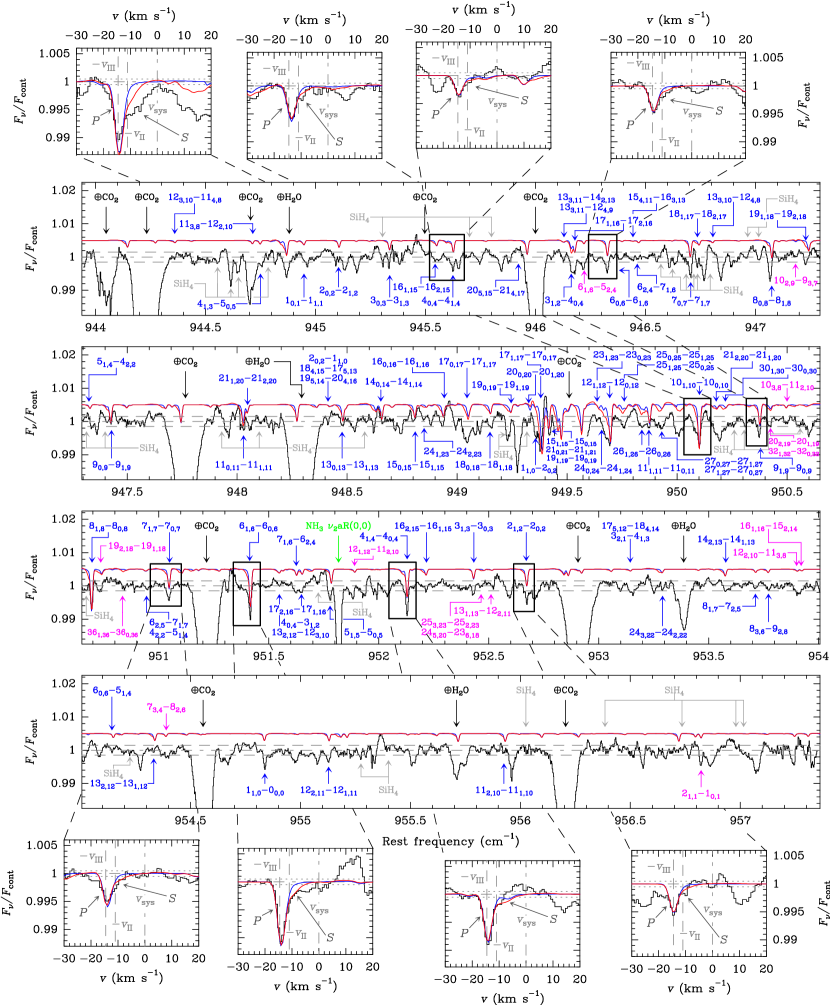
Figure 1.— Observed spectrum against rest frequency. The spectral resolution is $\simeq 3$ km s^-1. The gray dashed-dot and dashed horizontal lines indicate the continuum and the detection limit ($3\sigma\simeq 0.15\%$). The labels of the telluric lines are plotted in black. The lines of C₂H₄ and NH₃ produced in the envelope of IRC+10216 undoubtedly identified are plotted in blue and green, respectively. The features labeled with magenta comprises C₂H₄ lines that could be fully blended with other unknown lines or are tentative identifications. The spectrum also contains a number of SiH₄ lines plotted in gray. The synthetic spectrum of C₂H₄ is plotted in blue (C₂H₄ only in Region II; Scenario 1, see Table 2) and red (C₂H₄ in Regions II and III; Scenario $2A$). The $P$ and $S$ labels indicate the primary and secondary absorptions (see text).

Examination of the spectra showed that the ethylene lines are indeed very weak as reported more than 30 years ago by Betz (1981) and a few years later by Goldhaber et al. (1987). Typical depths of the strongest lines are less than 1% of the continuum. To improve the S/N, additional time was obtained in the 2008 observing season. This data were obtained in the same way as 2007 but only covered the 944 to 959 cm^-1 region. The signal-to-noise of the 2007 and 2008 spectra was similar so the two years were combined into the final observed spectrum. We estimate the RMS of the random noise of the spectrum to be $\simeq 0.05\%$ of the continuum emission.

The observed spectrum is not corrected for telluric contamination, which accounts for the strongest and prominent lines of CO₂ and H₂O (Fig. 1). Although weaker telluric lines are also present blocking some features coming from IRC+10216, 80 C₂H₄ lines of the fundamental band $\nu_{7}$ with $J\leq 30$ have been detected. About 35% of them are not blended and can be properly analyzed. Although several lines of the fundamental bands $\nu_{4}$ and $\nu_{10}$ fall within the observed spectral range, none of the lines of these bands is above the detection limit ($3\sigma\simeq 0.15\%$ of the continuum). No lines of hot or combination bands of the normal mode $\nu_{7}$ (e.g., $2\nu_{7}-\nu_{7}$ and $\nu_{7}+\nu_{10}-\nu_{10}$) have been found above the detection limit in this spectral range, either. These lines involve ro-vibrational levels with energies $\gtrsim 1200$ K (e.g. Oomens et al., 1996), barely populated in the mid and outer envelope where C₂H₄ is expected to exist (Cherchneff & Barker, 1992). In addition to C₂H₄ and telluric lines, we were able to identify the $\nu_{2}$ aR(0,0) line of NH₃ at 951.8 cm^-1 and a number of lines from SiH₄ between 944 and 947 cm^-1 (Gray et al., 1977; Pierre et al., 1986).

We used the low spectral resolution ISO/SWS observations carried out on 1996 May 31 (Cernicharo et al., 1999) to determine the properties of the dusty envelope. The uncertainty of these observations due to noise and the calibration process is estimated to be $\simeq 10\%$.

3. C₂H₄ spectroscopic constants

The rest frequencies of the observed ethylene lines and their intensities were taken from the HITRAN Database 2012 (Rothman et al., 2013). C₂H₄ is an asymmetric top molecule with 12 vibrational modes. Only the infrared active fundamental bands $\nu_{10}$, $\nu_{7}$, and $\nu_{4}$, with energies of 825.9, 948.8, and 1025.6 cm^-1, have lines in the observed range (e.g., Ulenikov et al., 2013). The $\nu_{7}$ band detected in our spectra corresponds to the out-of-plane bending mode.

The partition function was computed by direct summation over all the rotational levels with $J\lesssim 40$ of a number of vibrational states. The energy of the vibrational states and the rotational constants involved in the calculation of the partition function ($E_{\textnormal{\scriptsize{vib}}}\lesssim 5200$ K) were retrieved from the HITRAN Database 2012, Oomens et al. (1996), Sartakov et al. (1997), Willaert et al. (2006), Loroño-González et al. (2010), Lafferty et al. (2011), Lebron & Tan (2013a), Lebron & Tan (2013b), Lebron & Tan (2013c), and Ulenikov et al. (2013). The energy of the rotational levels for each vibrational state was calculated by diagonalizing the Watson’s Hamiltonian in its A-reduction $I^{r}$ representation, suitable to describe the C₂H₄ rotational structure (e.g., Lebron & Tan, 2013a; Ulenikov et al., 2013). The number of vibrational states required to calculate the partition function in warm regions of the envelope is less than 5 while up to some tens were necessary in hotter regions. The partition function calculated under local thermodynamical equilibrium (LTE) and a kinetic temperature of 296 K is $1.09\times 10^{4}$, in very good agreement with previous calculations (Blass et al., 2001; Rothman et al., 2013).

The optical constants needed to calculate the opacity of dust grains were taken from Rouleau & Martin (1991) for amorphous carbon and from Mutschke et al. (1999) for SiC.

4. Modeling

The modeling process was done with the code developed by Fonfría et al. (2008), which numerically solves the radiation transfer equation of a spherically symmetric envelope composed of gas and dust in radial expansion. It was successfully used to analyzed the mid-IR spectra of C₂H₂, HCN, SiS, C₄H₂, and C₆H₂ at 8 and $13~{}\mu$m towards IRC+10216 and the proto-planetary nebula CRL618 (Fonfría et al., 2008, 2011, 2015). A detailed description of the code can be found in Fonfría et al. (2008) and Fonfría et al. (2014).

In order to analyze the C₂H₄ lines identified in the spectrum, we adopted the envelope structure and expansion velocity field derived by Fonfría et al. (2015) from the modeling of the SiS emission. The envelope is composed of three Regions (I, II, and III) ranging from 1 to 5$R_{\star}$, from 5 to 20$R_{\star}$, and from 20$R_{\star}$ up to the external radius of the envelope, $R_{\textnormal{\scriptsize{ext}}}$. This parameter was fixed to 500$R_{\star}$, a distance compatible with the position where C₂H₄ is believed to be dissociated (e.g., Glassgold, 1996; Guélin et al., 1997; Agúndez & Cernicharo, 2006). It is also large enough to prevent the uncertainties of the synthetic absorption components of the lines and of the calculated continuum emission to be above the noise RMS of our data. The gas expansion velocity field, $v_{\textnormal{\scriptsize{exp}}}$, comprises a linear increment between 1 and 11 km s^-1 along Region I and two zones matching up with Regions II and III where the gas expands at a constant velocity of 11 and 14.5 km s^-1, respectively (Table 1). The adopted line width is assumed to be 5 km s^-1 at the stellar photosphere, following the power-law $\propto 1/r$ up to 5$R_{\star}$ and remaining equal to 1 km s^-1 further away (Agúndez et al., 2012). The gas density and rotational and vibrational temperature profiles are assumed to follow the laws $\propto r^{-2}v_{\textnormal{\scriptsize{exp}}}^{-1}$ and $r^{-\gamma}$, respectively, where $\gamma$ could be different for the rotational and vibrational temperatures. No dust has been considered to exist in Region I. Throughout the rest of the envelope we have adopted dust grains composed of amorphous carbon (AC) and SiC with a size of $0.1~{}\mu$m and a density of 2.5 g cm^-3.

Table 1Non-free parameters in the fits of lines of C₂H₄

Parameter	Units	Value	Ref.
$D$	pc	123	1
$\alpha_{\star}$	arcsec	0.02	2
$R_{\star}$	cm	$3.7\times 10^{13}$
$\dot{M}$	M⊙ yr-1	$2.1\times 10^{-5}$	3
$T_{\star}$	K	$2330$	2
$R_{\textnormal{\scriptsize{in}}}$	$R_{\star}$	$5$	3
$R_{\textnormal{\scriptsize{out}}}$	$R_{\star}$	$20$	3
$v_{\textnormal{\scriptsize{exp}}}(1R_{\star}\leq r<R_{\textnormal{\scriptsize{in}}})$	km s-1	$1+2.5(r/R_{\star}-1)$	4
$v_{\textnormal{\scriptsize{exp}}}(R_{\textnormal{\scriptsize{in}}}\leq r<R_{\textnormal{\scriptsize{out}}})$	km s-1	$11.0$	3
$v_{\textnormal{\scriptsize{exp}}}(r\geq R_{\textnormal{\scriptsize{out}}})$	km s-1	$14.5$	3
$T_{\textnormal{\scriptsize{K}}}(R_{\star}\leq r<9R_{\star})$	K	$T_{\star}(R_{\star}/r)^{0.58}$	5
$T_{\textnormal{\scriptsize{K}}}(9R_{\star}\leq r<65R_{\star})$	K	$T_{\textnormal{\scriptsize{K}}}(9R_{\star})(9R_{\star}/r)^{0.40}$	5
$T_{\textnormal{\scriptsize{K}}}(r\geq 65R_{\star})$	K	$T_{\textnormal{\scriptsize{K}}}(65R_{\star})(65R_{\star}/r)^{1.2}$	5
$\Delta v(1R_{\star}\leq r<R_{\textnormal{\scriptsize{in}}})$	km s-1	$5\left(R_{\star}/r\right)$	6
$\Delta v(r\geq R_{\textnormal{\scriptsize{in}}})$	km s-1	$1$	6
$f_{\textnormal{\scriptsize{AC}}}$	%	95	3
$f_{\textnormal{\scriptsize{SiC}}}$	%	5	3
$\tau_{\textnormal{\scriptsize{dust}}}(11~{}\mu$m)		0.70	4
$T_{\textnormal{\scriptsize{dust}}}(R_{\textnormal{\scriptsize{in}}})$	K	825	4
$\gamma_{\textnormal{\scriptsize{dust}}}$		0.39	4

Note. — $D$: distance to the star; $\alpha_{\star}$: angular stellar radius; $R_{\star}$: linear stellar radius; $\dot{M}$: mass-loss rate; $T_{\star}$: stellar effective temperature; $R_{\textnormal{\scriptsize{in}}}$ and $R_{\textnormal{\scriptsize{out}}}$: position of the outer boundaries of Regions I and II; $v_{\textnormal{\scriptsize{exp}}}$: gas expansion velocity; $\Delta v$: line width; $f_{\textnormal{\scriptsize{X}}}$: fraction of dust grains composed of material X; $\tau_{\textnormal{\scriptsize{dust}}}$: dust optical depth along the line-of-sight; $T_{\textnormal{\scriptsize{dust}}}$: temperature of dust grains; $\gamma_{\textnormal{\scriptsize{dust}}}$: exponent of the decreasing dust temperature power-law ($\propto r^{-\gamma_{\textnormal{\scriptsize{dust}}}}$). References: (1) Groenewegen et al. (2012) (2) Ridgway et al. (1988) (3) Fonfría et al. (2008) (4) Fonfría et al. (2015) (5) De Beck et al. (2012) (6) Agúndez et al. (2012).

4.1. Fitting procedure

The fitting procedure is based on the minimization of the $\chi^{2}$ function defined as

$$\chi^{2}=\frac{1}{n-p}\sum_{i=1}^{n}w_{i}\left[\left(\frac{F_{\nu}}{F_{\textnormal{\scriptsize{cont}}}}\right)_{\textnormal{\scriptsize{obs,$i$}}}-\left(\frac{F_{\nu}}{F_{\textnormal{\scriptsize{cont}}}}\right)_{\textnormal{\scriptsize{synth,$i$}}}\right]^{2},$$ (1)

where $n$ and $p$ are the number of frequency channels and free parameters involved in the fitting process, $(F_{\nu}/F_{\textnormal{\scriptsize{cont}}})_{\textnormal{\scriptsize{synth}}}$ and $(F_{\nu}/F_{\textnormal{\scriptsize{cont}}})_{\textnormal{\scriptsize{obs}}}$ are the flux normalized to the continuum for the synthetic and observed spectra, and $w$ is a weight included for convenience (see Section 4.2). We assumed a number of physical parameters related to the envelope model as fixed during the fitting process (gas expansion velocity field, H₂ density, kinetic temperature, and terminal line width, among others; see Tables 1 and 2). The physical and chemical quantities related to C₂H₄ derived from the fits are the abundance with respect to H₂, the rotational temperature at 20$R_{\star}$, and the exponent of the power-law followed by the rotational temperature beyond 20$R_{\star}$. All of the free parameters have been varied until the whole set of lines has been best fitted at the same time. The uncertainties of the free parameters have been estimated by simultaneously varying all of them until the synthetic spectrum departs at any frequency in more than the observational errors from the best global fit.

Table 2Derived Parameters

Parameter	Units	Value	Error	Value	Error	Value	Error
		Scenario 1		Scenario 2
				Case A		Case B
$\chi_{d}^{2}$	$\times 10^{-2}$	4.97	—	3.84	—	3.92	—
$\chi_{\textnormal{\scriptsize{red}}}^{2}$		7.02	—	3.80	—	4.08	—
$x(R_{\star}\leq r\leq R_{\textnormal{\scriptsize{in}}}^{-})$	$\times 10^{-8}$	0.0	—	0.0	—	0.0	—
$x(r=R_{\textnormal{\scriptsize{in}}}^{+})$	$\times 10^{-8}$	0.0	—	6.9	$+1.9/-1.8$	0.0	—
$x(r=R_{\textnormal{\scriptsize{out}}}^{-})$	$\times 10^{-8}$	0.0	—			11.0	$+3.3/-2.6$
$x(r\geq R_{\textnormal{\scriptsize{out}}}^{+})$	$\times 10^{-8}$	8.2	$+1.1/-1.2$	8.2	$+1.3/-1.1$	8.2	$+1.3/-1.0$
$T_{\textnormal{\scriptsize{rot}}}(R_{\star})$	K	2330∗	—	2330∗	—	2330∗	—
$T_{\textnormal{\scriptsize{rot}}}(R_{\textnormal{\scriptsize{in}}})$	K	916∗	—	916∗	—	916∗	—
$T_{\textnormal{\scriptsize{rot}}}(R_{\textnormal{\scriptsize{out}}})$	K	370	$+60/-80$	380	$+65/-60$	380	$\pm 60$
$\gamma_{\textnormal{\scriptsize{rot}}}$		0.54	$\pm 0.04$	0.54†	—	0.54†	—
$T_{\textnormal{\scriptsize{vib}}}(R_{\star})$	K	2330‡	—	2330‡	—	2330‡	—
$T_{\textnormal{\scriptsize{vib}}}(R_{\textnormal{\scriptsize{in}}})$	K	500‡	—	500‡	—	500‡	—
$T_{\textnormal{\scriptsize{vib}}}(R_{\textnormal{\scriptsize{out}}})$	K	315‡	—	315‡	—	315‡	—
$\gamma_{\textnormal{\scriptsize{vib}}}$		1.0‡	—	1.0‡	—	1.0‡	—
$N_{\textnormal{\scriptsize{col}}}(R_{\textnormal{\scriptsize{in}}}^{+}\leq r\leq R_{\textnormal{\scriptsize{out}}}^{-})$	$\times 10^{15}$ cm-2	0.0	—	5.8	$+1.6/-1.5$	2.5	$+0.8/-0.6$
$N_{\textnormal{\scriptsize{col}}}(r\geq R_{\textnormal{\scriptsize{out}}}^{+})$	$\times 10^{15}$ cm-2	1.66	$+0.22/-0.24$	1.67	$+0.26/-0.22$	1.67	$+0.26/-0.20$
$N_{\textnormal{\scriptsize{col,total}}}$	$\times 10^{15}$ cm-2	1.66	$+0.22/-0.24$	7.5	$+1.9/-1.7$	4.2	$+1.1/-0.8$

Note. — $\chi_{d}^{2}$ and $\chi_{\textnormal{\scriptsize{red}}}^{2}$: minimum of the $\chi^{2}$ function (Eq. 1) assuming the weights $w=1/d^{2}$ and $1/\sigma^{2}$, where $d$ is the depth of each line and $\sigma$ is the noise RMS of the spectrum ($\chi_{\textnormal{\scriptsize{red}}}^{2}$ is the reduced $\chi^{2}$ function); $x$: abundance relative to H₂; $R_{\textnormal{\scriptsize{in}}}^{+}$ and $R_{\textnormal{\scriptsize{in}}}^{-}$: $R_{\textnormal{\scriptsize{in}}}$ approached from Region II and Region I, respectively; $R_{\textnormal{\scriptsize{out}}}^{+}$ and $R_{\textnormal{\scriptsize{out}}}^{-}$: $R_{\textnormal{\scriptsize{out}}}$ approached from Region III and Region II, respectively; $T_{\textnormal{\scriptsize{rot}}}$: rotational temperature; $\gamma_{\textnormal{\scriptsize{rot}}}$: exponent of the rotational temperature power-law outwards from $R_{\textnormal{\scriptsize{out}}}^{+}$ ($\propto r^{-\gamma_{\textnormal{\scriptsize{rot}}}}$); $T_{\textnormal{\scriptsize{vib}}}$: vibrational temperature derived from band $\nu_{7}$; $\gamma_{\textnormal{\scriptsize{vib}}}$: exponent of the vibrational temperature power-law outwards from $R_{\textnormal{\scriptsize{out}}}$ ($\propto r^{-\gamma_{\textnormal{\scriptsize{vib}}}}$); $N_{\textnormal{\scriptsize{col}}}$: C₂H₄ column density calculated with the parameters derived from the best fits to the observations. The parameters for which no uncertainty has been provided (—) were assumed as fixed during the whole fitting process. The errors are 1-sigma uncertainties for all the parameters. ^∗This rotational temperature was fixed to the kinetic temperature derived by De Beck et al. (2012). ^†This value was fixed to the result derived from the fit to the observed lines assuming Scenario 1. ^‡The vibrational temperature for C₂H₄ was fixed to the vibrational temperature derived by Fonfría et al. (2008) from the analysis of the C₂H₂ lines of band $\nu_{5}$. A blank cell contains the same value than the immediately upper cell.

4.2. Weighting the $\chi^{2}$ function

The strongest lines identified in the spectrum are those with $J\lesssim 15$ (Fig. 1). The formation of C₂H₄ in the different regions of the envelope could be influenced by variations in the physical and chemical conditions between the stellar photosphere and $\simeq 50$$R_{\star}$ (Fonfría et al., 2014, 2015), probably related to the binary nature of the central stellar system (Cernicharo et al., 2015a, 2016; Decin et al., 2015; Kim et al., 2015; Quintana-Lacaci et al., 2016). This means that the difference between the strongest observed and synthetic lines could be as large as the depth of the absorption component of the weakest lines. This fact could result in an underestimation of the importance of the weakest lines (usually the highest excitation lines) during the automatic fitting procedure. Thus, the rotational temperature of the C₂H₄ enclosed by the inner shells of Region III would be lower than the actual one, being dominated by the temperature prevailing in the outer envelope.

This situation can be solved by adopting the weight $w=1/d^{2}$ for all the channels of each line, where $d$ is the depth of its absorption component. This choice gives a comparable importance during the fitting process to the weak lines formed at distances to the star $\lesssim 30R_{\star}$ and the strong lines mostly formed beyond, resulting in a more realistic rotational temperature profile. It is worth noting that the fit to the strong lines and the derived abundance profile throughout Region III are not significantly affected by the chosen weight.

It is also convenient to use the so-called reduced $\chi^{2}$ function, $\chi^{2}_{\textnormal{\scriptsize{red}}}$, to numerically estimate the goodness of the fits. Its definition involves a weight $w=1/\sigma^{2}$, where $\sigma$ is the uncertainty of the observed data, and the number of degrees of freedom of the fit, usually defined as $n-p$, where $n$ is the number of points of the set to fit and $p$ the number of parameters varied during the fitting process. In theory, $\chi_{\textnormal{\scriptsize{red}}}^{2}$ approaches to 1 for a good fit to a set of experimental data, adopting larger values for worse fits. In practice, it is difficult to use $\chi_{\textnormal{\scriptsize{red}}}^{2}$ to figure out the actual quality of a given fit but it can be used to compare different fits (e.g., Taylor, 1997; Tallon-Bosc et al., 2007).

4.3. Deviations of the synthetic spectrum from the observed one

The fit to the observed spectrum was improved by slightly shifting the frequency of several observed C₂H₄ lines. All of these shifts are smaller than 2.5 km s^-1 ($\simeq 0.007$ cm^-1) depending on the chosen model (see Section 5.1). These differences can be explained by the spectral resolution of our data, estimated to be $\simeq 3$ km s^-1. However, the deviation between the synthetic and observed profiles of some lines such as, e.g., $1_{1,0}-0_{0,0}$ and $8_{1,8}-8_{0,8}$ (2 and 3.5 times smaller and larger, respectively), are unexpectedly large while other lines involving ro-vibrational states with similar or intermediate energies are well reproduced (e.g., $2_{1,2}-2_{0,2}$, $6_{0,6}-6_{1,6}$, $9_{1,9}-9_{0,9}$). The observed feature identified as line $1_{1,0}-0_{0,0}$ could be stronger than expected due to an unnoticed blending with other unknown lines or a cold contribution not included in our model. Nevertheless, the fact that the observed $8_{1,8}-8_{0,8}$ line is weaker than the synthetic one while other lines formed in the same region of the envelope are better reproduced suggests that, probably, the baseline was not well removed around this line. This problem usually appears when the number of molecular features in the vicinity of the target line is high, hiding the actual baseline.

5. Results and discussion

About 35% of the detected lines have well enough defined profiles to be fitted. Most lines show an absorption component. A systematic emission component is not obvious in the data. Some lines showing a possible emission component are probably affected by the baseline removal. The absorption component of the strong lines is usually dominated by a deep, narrow contribution at $\simeq-14$ km s^-1 (primary absorption, $P$ in the insets of Fig. 1), presumably caused by the gas expanding at the terminal velocity, and a red-shifted weaker contribution (secondary absorption, $S$ in the insets of Fig. 1). These secondary absorptions could be argued to be other lines of the same band or of a hot band. In fact, some strong lines of the $\nu_{7}$ band are accompanied by close, weaker lines of the same band that influence their profiles. However, these C₂H₄ line sets are not so common and the frequency shift between the primary and the secondary absorptions remains nearly constant for every observed strong line. This would be an unexpected behavior if the secondary absorptions were other C₂H₄ lines. The Doppler velocity of the secondary absorptions is more compatible with the features produced by the gas in Region II expanding at $\simeq 11$ km s^-1. This reasoning is supported as well by the existence of weak lines involving ro-vibrational levels with energies up to $\simeq 800$ cm^-1 ($\simeq 1150$ K) that are expected to be significantly excited inwards from $\simeq 20$$R_{\star}$, where the kinetic temperature is $\gtrsim 470$ K (De Beck et al., 2012). On the other hand, the lack of an evident emission component in the observed lines and, particularly, in lines involving lower ro-vibrational levels with energies $\gtrsim 1200$ K suggest that the C₂H₄ abundance is negligible from the stellar surface up to the middle shells of Region II ($\simeq 10-15$$R_{\star}$). This spatial distribution is roughly consistent with the predicted by thermodynamical chemical equilibrium models (e.g., Cherchneff & Barker, 1992), which suggest that C₂H₄ reaches a significant abundance in shells with a kinetic temperature $\gtrsim 1000$ K (closer to the star than 5$R_{\star}$ in our envelope model).

Figure 2.— Ro-vibrational diagram of the observed C₂H₄ lines. The lines are separated into two different groups: warm lines (blue dots) and hot lines (red triangles). The warm lines are those involving lower ro-vibrational levels with energies below 177 K. The hot lines involve lower levels with higher energies. These groups of lines were linearly fitted separately following Eq. 2 to derive their rotational temperatures, $T_{\textnormal{\scriptsize{rot}}}$, and their column densities, $N_{\textnormal{\scriptsize{col}}}$.

A quantitative analysis can be obtained through a ro-vibrational diagram (see Fig. 2). In this plot, we take advantage of the absence of an emission component of the lines. When such emission is present, it overlaps the absorption component of the profile requiring the application of complex envelope models to derive reliable information about the circumstellar gas (e.g., Keady et al., 1988; Keady & Ridgway, 1993; Boyle et al., 1994; Fonfría et al., 2008, 2015). The general weakness of the observed C₂H₄ lines, with depths of their absorption components below $\simeq 1\%$ of the continuum, suggest that they are all optically thin and the following formula holds:

$$\ln{\left[\frac{I\nu^{2}8\pi c}{A_{ul}g_{u}N_{\textnormal{\scriptsize{col,0}}}}\right]}\simeq\ln{\left[\frac{N_{\textnormal{\scriptsize{col}}}}{N_{\textnormal{\scriptsize{col,0}}}Z}\frac{\theta_{s}^{2}}{\theta_{s}^{2}+\theta_{b}^{2}}\right]}-\frac{hcE_{\textnormal{\scriptsize{low}}}}{k_{\textnormal{\scriptsize{B}}}T_{\textnormal{\scriptsize{rot}}}}$$ (2)

where $\nu$ is the rest frequency of each line (cm^-1), $I$ is the integral of the normalized flux absorbed by each line over the frequency ($\int_{\textnormal{\scriptsize{line}}}\left(1-F_{\nu}/F_{\textnormal{\scriptsize{cont}}}\right)d\nu$; cm^-1), $A_{ul}$ the A-Einstein coefficient of the transition (s^-1), $g_{u}$ the degeneracy of the upper level of the transition, $Z$ is the partition function, $c$ the velocity of light in vacuum (cm s^-1), $N_{\textnormal{\scriptsize{col}}}$ the column density of C₂H₄ (cm^-2), $E_{\textnormal{\scriptsize{low}}}$ the energy of the lower ro-vibrational level involved in the transition (cm^-1), $h$ and $k_{\textnormal{\scriptsize{\tiny B}}}$ are the Planck and Boltzmann constants, and $T_{\textnormal{\scriptsize{rot}}}$ the rotational temperature (K). $N_{\textnormal{\scriptsize{col,0}}}=10^{15}$ cm^-2 is a fixed column density included for convenience to get a dimensionless argument for the logarithms. In this equation, we assume the rotational temperature is low enough that $e^{-hc\nu/k_{\textnormal{\scriptsize{\tiny B}}}T_{\textnormal{\scriptsize{\tiny rot}}}}\ll 1$. The factor $\theta_{s}^{2}/(\theta_{s}^{2}+\theta_{b}^{2})$, where $\theta_{s}$ is the angular size of the source and $\theta_{b}$ the HPBW of the IRTF ($\simeq 0\farcs 9$ at 10.5 $\mu$m), accounts for the effect of the size differences between the source and the main beam of the PSF. The size of the source can be roughly estimated with the aid of our code assuming the parameters of Table 1 and that ethylene is under LTE. This approximation gives that $\theta_{s}\simeq 1\farcs 9\pm 0\farcs 2$, which means that $\theta_{s}^{2}/(\theta_{s}^{2}+\theta_{b}^{2})\simeq 0.82\pm 0.03$.

The data plotted in Fig. 2 suggest that the observed lines belong to two different populations. We will refer to them as warm and hot lines, hereafter. The data related to each population were separately fitted adopting the typical weight based on the statistical uncertainties of the line intensities. The warm lines involve lower ro-vibrational levels with energies below $\simeq 180$ K and show a rotational temperature of $105\pm 30$ K, compatible with the preliminary result proposed by Hinkle et al. (2008). Adopting the envelope model described in Section 4 and LTE, these lines would be mostly formed at distances to the star of $\simeq 125-200R_{\star}$ ($\simeq 2\farcs 5-4\farcs 0$). On the other hand, the hot lines are formed in shells where the physical conditions favor a higher rotational temperature ($T_{\textnormal{\scriptsize{rot}}}=400\pm 80$ K). Thus, these shells would be located at $\simeq 20-50R_{\star}$ ($\simeq 0\farcs 4-1\farcs 0$) from the star. This means that the existence of a significant abundance of C₂H₄ in Region I, i.e., between the stellar photosphere and 5$R_{\star}$, can be ruled out. The total column density derived from the ro-vibrational diagram is $(6.5\pm 1.7)\times 10^{15}$ cm^-2 compatible with the rough estimations by Betz (1981) and Goldhaber et al. (1987), i.e., $\sim 10^{16}$ and $4\times 10^{15}$ cm^-2, respectively, which are affected by an error of one order of magnitude. About 75% of the C₂H₄ column density is enclosed by the shell at 20$R_{\star}$ while only $\simeq 25\%$ of it is related to the ethylene spread at larger distances.

5.1. Abundance with respect to H₂

In order to describe the C₂H₄ abundance profile we attempted a synthesis of the observed lines assuming two different scenarios: (1) C₂H₄ only exists in Region III and (2) C₂H₄ exists in Regions II and III. Scenario 2 is further broken down into two sub-scenarios, $A$ and $B$, where we assumed that the abundance is constant throughout Regions II and III (Scenario $2A$) and it is constant in Region III, growing linearly from 0 across Region II up to an abundance that could be different than that of Region III (Scenario $2B$). In both Scenarios $2A$ and $2B$ the abundance was not necessarily a continuous profile. The results of the analysis of all these scenarios can be found in Table 2.

The synthetic spectrum that fits the observations worst is from Scenario 1 with $\chi_{\textnormal{\scriptsize{red}}}^{2}\simeq 7.0$ (see Table 2). This scenario is capable of reproducing fairly well the primary absorption of the observed lines but it fails to describe their secondary absorptions and the high excitation lines. Scenarios $2A$ and $2B$ explain better the shape of the strong lines by adding a secondary absorption, reproducing at the same time the high excitation lines. The synthetic spectra calculated for both show an average $\chi_{\textnormal{\scriptsize{red}}}^{2}\simeq 4.0$, significantly smaller than for Scenario 1. None of these scenarios are able to fit the observations with $\chi_{\textnormal{\scriptsize{red}}}^{2}\simeq 1.0$, which would mean a perfect correlation between the observations and the synthetic spectrum. This fact indicates that the actual abundance distribution is likely more complex than we have assumed here. The shape of the secondary absorption of the strongest lines, which are usually deeper and narrower than seen in the synthetic spectra, might indicate that the solid angle subtended by the absorbing region around 20$R_{\star}$ is smaller than expected for a spherically symmetric abundance distribution. Consequently, there is an absorption deficit close to the systemic velocity (0 km s^-1 in the insets of Fig. 1) in the observed lines with respect to the synthetic features. This asymmetry in the abundance distribution could be related to those that Fonfría et al. (2014) invoked to explain the high angular resolution interferometer observations of H¹³CN, SiO, and SiC₂ at 1.2 mm or to the small scale features related to the spiral structure recently found in the envelope of IRC+10216 (Cernicharo et al., 2015a, 2016; Quintana-Lacaci et al., 2016).

The C₂H₄ abundance with respect to H₂ throughout Region III derived from our best fit is $(8.2\pm 1.3)\times 10^{-8}$ for all the Scenarios (1, $2A$, and $2B$; see Figure 3), which means a column density of $(1.7\pm 0.3)\times 10^{15}$ cm^-2. This column density is in very good agreement with the value derived from the linear fit to the warm lines in the ro-vibrational diagram [$(1.7\pm 0.4)\times 10^{15}$ cm^-2; Fig. 2]. The C₂H₄ abundance profile in Region II can be roughly explained by the two Scenarios $2A$ and $2B$. Although Scenario $2A$ best reproduces the observations with $\chi_{\textnormal{\scriptsize{red}}}^{2}\simeq 3.8$, the synthetic spectrum calculated assuming Scenario $2B$ shows a $\chi_{\textnormal{\scriptsize{red}}}^{2}$ only 7% higher. The abundance derived from Scenarios $2A$ and $2B$ in Region II are compatible. However, Scenario $2B$ enhances the absorption of lines involving low energy ro-vibrational levels formed in the outer shells of Region II at the expense of the absorption of higher excitation lines, formed closer to the star. Scenario $2A$ results in stronger high excitation lines but the difference with the same lines calculated with Scenario $2B$ is always below the noise RMS of the observed spectrum. These facts suggest that both Scenarios are similarly possible and we are barely sensitive to the absorption produced in the inner half of Region II. The column density in Region II derived from the hot lines of the ro-vibrational diagram [$(4.8\pm 1.3)\times 10^{15}$ cm^-2; Fig. 2] is between the values derived from Scenarios $2A$ and $2B$ [$(5.8\pm 1.6)$ and $(2.5\pm 0.8)\times 10^{15}$ cm^-2, respectively; Table 2], which indicates that the best scenario seems to be closer to Scenario $2A$, although it could also be a mix of both since the differences are not particularly significant. Thus, the actual abundance could be constant in the outer half (or a larger fraction) of Region II, linearly increasing in the inner half. In any case, the resulting spectrum would differ to those derived from Scenarios $2A$ and $2B$ in less than the noise RMS and would not throw any further light on the problem.

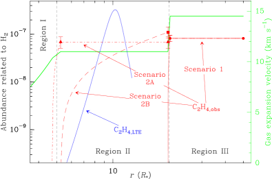
Figure 3.— Ethylene abundance with respect to H₂. The profiles derived for Scenarios 1, $2A$, and $2B$ are plotted in red (solid, dash-dotted, and dashed, respectively). A synthetic profile calculated with a chemical model under TE (see text) is plotted in blue. The adopted gas expansion velocity profile is plotted in green.

In a circumstellar envelope of an AGB star with a ratio C/O $\simeq 2$, such as IRC+10216 (e.g., Agúndez & Cernicharo, 2006), C₂H₄ is expected to form under thermal equilibrium (TE) near the stellar photosphere with a very low abundance with respect to H₂ ($\sim 10^{-15}$; e.g., Cherchneff & Barker, 1992). The abundance increases when the kinetic temperature decreases reaching a terminal value that keeps constant up to the outer envelope, where C₂H₄ is dissociated by the Galactic UV radiation. The position where the terminal abundance is reached and its value are hard to calculate since the thermal equilibrium condition seems to hold only from the stellar photosphere up to $\simeq 3-7R_{\star}$ (Cernicharo et al., 2010, 2013; Fonfría et al., 2014). Kinetic chemistry models required to make predictions at larger distances from the star are substantially affected by the uncertainties related to the kinetic constants involved in the chemical reaction network and the complexity of the calculations.

Table 3Previous estimates of the terminal C₂H₄ abundance/column density

$x$ ($\times 10^{-8}$)	$N_{\textnormal{\scriptsize{col,total}}}$ ($\times 10^{15}$ cm-2)	Method	Reference
$5.5^{*}-8.2$	$4.2-7.5$	Obs.	1
10	$10-100$	Obs.	2
$1-2^{\dagger}$	$4-40$	Obs.	3
30‡	—	Model	4
0.1	—	Model	5
0.2	0.001	Model	6

Note. — $x$: maximum terminal C₂H₄ abundance with respect to H₂; $N_{\textnormal{\scriptsize{col,total}}}$: total C₂H₄ column density; Method: derived from observations (Obs.) or from a chemical model (Model); References: (1) This work (beyond 20$R_{\star}$) (2) Betz (1981) (3) Goldhaber et al. (1987) (4) Cherchneff & Barker (1992) (5) Doty & Leung (1998) (6) Millar et al. (2000). ^∗This value is the average abundance of Scenario $2B$. ^†This value has been calculated with the aid of the CO abundances with respect to H₂ adopted by Keady et al. (1988) and De Beck et al. (2012). ^‡This abundance corresponds to a C-rich AGB star with C/O $\simeq 1.5-3.0$.

There are only a few estimates for the C₂H₄ column density or the abundance with respect to H₂ derived from observations or calculated using chemical models for IRC+10216 in the literature to compare with our results (see Table 3). The lower limit of the column density derived by Betz (1981) and Goldhaber et al. (1987) are compatible with our results within a factor of 2. These authors considered an error of one order of magnitude to account for the effect of the dust emission on the C₂H₄ lines. However, this uncertainty is too big because the optical depth of the dust is $\simeq 0.75$ at $\simeq 10.5~{}\mu$m (Table 1). In fact, this effect exists but it is much less important than they considered. The chemical model by Millar et al. (2000) gives a very low column density in part because their model produces ethylene in the outer envelope, where the gas density is orders of magnitude lower than at in the inner layers of the CSE. This is the same reason that the abundance with respect to H₂ predicted in Millar et al. (2000) and Doty & Leung (1998) are about two orders of magnitude lower than ours. The peak abundance calculated by Cherchneff & Barker (1992) for a C-rich AGB star with C/O $\simeq 1.5-3.0$ and assuming TE is a factor of 4 to 6 higher than our estimate. This disagreement could be related to the fact that their envelope model represents a typical AGB star different than IRC+10216. However, our abundance is in good agreement with that proposed by Betz (1981), although these authors only estimated the order of magnitude. Interestingly, despite the compatibility existing between the column density derived in the current work and that of Goldhaber et al. (1987), the abundance proposed by these authors is at least 3 times lower than ours. This disagreement can be explained by the fact that they did not have any data related to the hot lines with a $T_{\textnormal{\scriptsize{rot}}}=400$ K that we have been able to detect due to the high S/N of our observed spectrum.

The comparison between the abundance of C₂H₄ with respect to H₂ and/or the column density we derive, and the results of the chemical models indicates that the ethylene formation process in IRC+10216 is still not well understood. The C₂H₄ abundances derived by Doty & Leung (1998) and Millar et al. (2000) are between one and two orders of magnitude lower than the observational results (Table 3). Additionally, these models suggest that ethylene is formed somewhere in the outer envelope while our observations reveal that it happens much closer to the central star. The differences between the model of the envelope used for these chemical kinetics calculations and the one adopted here (e.g., our mass-loss rate is lower by a factor of $\simeq 2-3$) is unlikely to be the reason of the discrepancy concerning C₂H₄. To our knowledge, no thermochemical equilibrium model of the surroundings of the star has provided predictions on the abundance of C₂H₄ in IRC+10216. We have therefore carried out TE calculations for IRC+10216 to check if the general predictions of Cherchneff & Barker (1992) can be improved for the particular case of IRC+10216, fitting better our observational results.

The chemical model we have adopted is the same that Fonfría et al. (2014) used to explain the abundances of H¹³CN, SiO, and SiC₂ in the inner layers of IRC+10216 derived from high spatial resolution observations. The resulting C₂H₄ abundance profile is compared with the abundance we derive from the observations in Figure 3. Unlike what happens for H¹³CN, SiO, and SiC₂, that reach maximum abundances within $\simeq 3-4R_{\star}$ from the star, the predicted peak abundance of C₂H₄ occurs somewhat farther from the star, at $\simeq 9R_{\star}$, in very good agreement with our observational results. In addition, this model improves the general results by Cherchneff & Barker (1992) indicating that it works reasonably well for abundant molecules (e.g., HCN or SiC₂) and for molecules such as C₂H₄ with an abundance as low as $\sim 10^{-8}-10^{-7}$.

On the other hand, the predicted peak abundance is more than 4 times higher than the value we derive from observations and the chemical model indicates that ethylene should vanish in a few stellar radii, something that does not happen according to our observations. This latter fact can be explained in terms of a freeze out of the TE abundance of C₂H₄ at radii beyond $\simeq 9R_{\star}$ as a consequence of the slow down of chemical reactions induced by the decrease in density and temperature. It still remains to be demonstrated whether chemical kinetics can actually be at work at distances from the star as large as $\simeq 9R_{\star}$ to drive the abundance of C₂H₄ to values of the order of $10^{-7}$ relative to H₂. Although observations of ethylene indicate that TE does indeed hold up to $\simeq 9R_{\star}$, a detailed chemical kinetics model dealing with the innermost circumstellar regions of IRC+10216 would be needed to shed light on this point from the theoretical point of view.

5.2. Vibrational and rotational temperatures

The vibrational temperature controls the number of molecules in the upper vibrational state, having a direct effect on the overall emission of the whole fundamental band $\nu_{7}$ and on the absorption component of the corresponding hot and combination bands (e.g., Fonfría et al., 2015). Hence, the absence of an obvious emission component in the observed lines and of lines of hot and combination bands above the detection limit prevents us from estimating this temperature. The inner limit of the region of the envelope where C₂H₄ is formed is too far from the star to allow for the development of significant emission components and high excitation lines. In this situation, the best choices are (1) to assume that C₂H₄ is under vibrational LTE or (2) to adopt the vibrational temperature profile of other molecules. It was shown that molecules such as HCN, C₂H₂, and SiS (Fonfría et al., 2008, 2015) are vibrationally out of LTE away from several stellar radii from the stellar photosphere so we expect this to happen to C₂H₄ as well. This is supported by the fact that the collisional rate coefficients involved in ro-vibrational transitions are expected to be several orders of magnitude smaller than in pure rotational transitions (e.g., Toboła et al., 2008).

Hence, a realistic approach would be to adopt the vibrational temperature of the IR active C₂H₂ fundamental band $\nu_{5}$. This is a reasonable choice since the adoption of a vibrational temperature only 10% higher produces lines with a small though significant emission component, unobserved in our data. The inaccuracy associated with this choice has implications on the uncertainties of the abundance, which are larger than showed in Table 2. A variation of 10% of the vibrational temperature at 5 or 20$R_{\star}$ modifies the abundance in $\simeq 2$ and 5%, respectively, while the same relative change of the exponent $\gamma_{\textnormal{\scriptsize{vib}}}$ results in a negligible variation of 0.5% of the abundance. Hence, an accurate determination of the C₂H₄ abundance would require a better estimation of the vibrational temperature mainly between 10 and 20$R_{\star}$.

The rotational temperature, $T_{\textnormal{\scriptsize{rot}}}$, was fixed to the kinetic one, $T_{\textnormal{\scriptsize{K}}}$, at 5$R_{\star}$, where the C₂H₄ abundance probably is very low and we have no reliable information about the excitation. However, the rotational temperature at 20$R_{\star}$ can be properly determined from the fits to the observations adopting a value of $\simeq 380$ K with an uncertainty of $\simeq 15\%$ (Table 2). Beyond this position, our best fit results in a power-law dependence $\propto r^{-0.54}$. A decrease of 50% in the rotational temperature at 5$R_{\star}$ only introduces changes in the synthetic spectrum up to the noise level ($\sigma=0.05\%$) so that the rotational temperature at 20$R_{\star}$ remains unaffected. The comparison between the rotational and the kinetic temperatures by De Beck et al. (2012) suggests that C₂H₄ could be rotationally out of LTE (Figure 4). However, if we compare $T_{\textnormal{\scriptsize{rot}}}$ with $T_{\textnormal{\scriptsize{K}}}$ taken from other works (Boyle et al., 1994; Schöier et al., 2007; Agúndez et al., 2012), the $1\sigma$ error intervals of $T_{\textnormal{\scriptsize{rot}}}$ and the actual $T_{\textnormal{\scriptsize{K}}}$ are overlapped. Thus, the deviation of the rotational temperature to the kinetic one is not significant and C₂H₄ can be assumed rotationally under LTE, as it is expected for a symmetric molecule with no permanent dipole moment.

This rotational temperature, that we have concluded to be very similar to the actual kinetic temperature, allows us to refine the zones of the envelope where the bulk absorption of the warm and hot lines found in the ro-vibrational diagram (Fig. 2) arise. The warm lines, with an average rotational temperature of $105\pm 30$ K, are mostly formed between 135 and 400$R_{\star}$ while the hot lines, with an average rotational temperature of $400\pm 80$ K, are formed between 14 and 28$R_{\star}$.

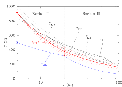
Figure 4.— Kinetic, vibrational, and rotational temperatures throughout the region of the envelope where the observed C₂H₄ lines seem to be formed. The kinetic temperatures $T_{\textnormal{\scriptsize{K}},i}$ (black) were taken from (1) De Beck et al. (2012), (2) Agúndez et al. (2012), (3) Schöier et al. (2007), and (4) Boyle et al. (1994). The vibrational temperature $T_{\textnormal{\scriptsize{vib}}}$ (blue) for the C₂H₄ $\nu_{7}$ band was assumed to be equal to the vibrational temperature for the $\nu_{5}$ band of C₂H₂ (Fonfría et al., 2008). The rotational temperature $T_{\textnormal{\scriptsize{rot}}}$ (red) has been derived from our analysis. The $1\sigma$ error interval of $T_{\textnormal{\scriptsize{rot}}}$ has been plotted as a striped region.

5.3. Ethylene and dust

Although the abundance profile in Region II derived from Scenario $2A$ is too rough to get information about the C₂H₄ depletion onto the dust grains, Scenario $2B$ suggests that it might happen at 20$R_{\star}$ with at most 25% of the abundance with respect to H₂ in the outer shells of Region II ($\simeq 1.1\times 10^{-7}$). This means that the density of C₂H₄ molecules in these shells that could condense is up to 0.9 cm^-3, implying an upper limit for the column density along 1$R_{\star}$ of $\simeq 3.3\times 10^{13}$ cm^-2. Thus, a 1$R_{\star}$ width shell with a radius of 20$R_{\star}$ contains up to $2.3\times 10^{44}$ C₂H₄ molecules, i.e., $1.1\times 10^{22}$ g of ethylene. Assuming that the total mass ejected from the star in form of dust is $\simeq 2.5\times 10^{-8}$ M_⊙ yr^-1 (De Beck et al., 2012; Decin et al., 2015), there is about $4.6\times 10^{25}$ g of dust in the shell defined above. Hence, the possible contribution of C₂H₄ to the dust mass around 20$R_{\star}$, where the gas seems to be accelerated from 11 to 14.5 km s^-1, would be $\lesssim 0.025\%$ corresponding to an increment of the size of the dust grains $\lesssim 0.02$%. This negligible growth cannot affect the gas and dust acceleration but the C₂H₄ condensation could enrich the chemistry on the surface of the grains.

6. Summary

High resolution observations ($R\simeq 100,000$) of the C₂H₄ band $\nu_{7}$ found in the $\simeq 10.5~{}\mu$m spectrum of IRC+10216 have been analyzed. Eighty C₂H₄ lines were found in the observations above the $3\sigma$ ($\simeq 0.15\%$ of the continuum) detection limit. Of these lines about 35% are unblended or partially blended allowing for a detailed analysis of their profiles with a rotational diagram and the code developed by Fonfría et al. (2008).

From these analyses, we conclude that:

• The C₂H₄ lines can be divided into two groups with significantly different rotational temperatures: a hot group with an rotational temperature of $\simeq 400$ K composed of lines located between $\simeq 14$ and 28$R_{\star}$ and a warm group with an rotational temperature of $\simeq 105$ K composed of lines mostly produced between $\simeq 135$ and 400$R_{\star}$. No evidence of C₂H₄ closer to the star than $\simeq 10$$R_{\star}$ was found.

• The C₂H₄ abundance profile with respect to H₂ is compatible with an average value of $6.9\times 10^{-8}$ between 5 and 20$R_{\star}$ and a terminal abundance of $8.2\times 10^{-8}$ beyond 20$R_{\star}$. This last value is at least 4 times larger than the chemical models predict. The terminal abundance seems not to depend on the chosen profile but the abundance closer to the star is probably more complex that we assumed, involving its growth between 5 and 10$R_{\star}$. The total C₂H₄ column density ranges from 4.2 to $7.5\times 10^{15}$ cm^-2.

• The rotational temperature derived from the fits to the observed lines is equal to the kinetic temperature at 5$R_{\star}$ ($\simeq 915$ K) and $\simeq 380$ K at 20$R_{\star}$, below the kinetic temperature ($\simeq 475$ K). At larger distances from the star the rotational temperature follows the power-law $\propto r^{-0.54}$. C₂H₄ can be considered rotationally under LTE throughout the region of the envelope traced with our observations.

• The vibrational temperature of the C₂H₄ band $\nu_{7}$ is unknown but it could be assumed to be similar to that of the C₂H₂ band $\nu_{5}$. In all cases, the good fits achieved with this temperature suggests that C₂H₄ is vibrationally out of LTE.

• A fraction of the gas-phase C₂H₄ could condense onto the dust grains around $\simeq 20R_{\star}$. The dust grains barely grow due to this depletion and no significant influence on the gas acceleration is expected to happen but the adsorbed C₂H₄ molecules could affect the chemistry evolution in the surface.

References

- Agúndez & Cernicharo (2006) Agúndez M. & Cernicharo J., 2006, ApJ, 650, 374
- Agúndez et al. (2010) Agúndez M., Cernicharo J. & Guélin M., 2010, ApJ, 724, L133
- Agúndez et al. (2012) Agúndez M., Fonfría J. P., Cernicharo J., Kahane C., Daniel F., & Guélin M., 2012, A&A, 543, A48
- Agúndez et al. (2014) Agúndez M., Cernicharo J. & Guélin M., 2014, A&A, 570, A45
- Bernath et al. (1989) Bernath P. F., Hinkle K. W. & Keady J. J., 1989, Sci, 244, 562
- Betz (1981) Betz A. L., 1981, ApJ, 244, L103
- Blass et al. (2001) Blass W. E. et al., 2001, J. Quant. Spec. Radiat. Transf., 71, 47
- Boyle et al. (1994) Boyle R. J., Keady J. J., Jennings D. E., Hirsch K. L. & Wiedemann G. R., 1994, ApJ, 420, 863
- Cernicharo et al. (1987) Cernicharo J. & Guélin M., 1987, A&A, 183, L10
- Cernicharo et al. (1989) Cernicharo J., Gottlieb C. A., Guélin M., Thaddeus P. & Vrtilek J. M., 1989, ApJ, 341, L25
- Cernicharo et al. (1999) Cernicharo J., Yamamura I., González-Alfonso E., de Jong T., Heras A., Escribano R., & Ortigoso J., 1999, ApJ, 526, L41
- Cernicharo et al. (2000) Cernicharo J., Guélin M., & Kahane C., 2000, A&AS, 142, 181
- Cernicharo (2004) Cernicharo J., 2004, ApJ, 608, L41
- Cernicharo et al. (2010) Cernicharo J. et al., 2010, A&A, 521, L8
- Cernicharo et al. (2013) Cernicharo J., Daniel F., Castro-Carrizo A., Agúndez M., Marcelino N., Joblin C., Goicoechea J. R. & Guélin M., 2013, ApJ, 778, L25
- Cernicharo et al. (2015a) Cernicharo J., Marcelino N., Agúndez M. & Guélin M., 2015, A&A, 575, A91
- Cernicharo et al. (2015b) Cernicharo J. et al., 2015b, ApJ, 806, L3
- Cernicharo et al. (2016) Cernicharo J., Castro-Carrizo A., Quintana-Lacaci G., Agúndez M., Marcelino N., Velilla Prieto L., Fonfría J. P. & Guélin M., 2016, submitted to the ApJ
- Cherchneff & Barker (1992) Cherchneff I. & Barker J. R., 1992, ApJ, 394, 703
- Cherchneff (2006) Cherchneff I., 2006, A&A, 456, 1001
- Contreras et al. (2011) Contreras C. S., Ricketts C. L. & Salama F., 2011, EAS Publication Series, 46, 201
- De Beck et al. (2012) De Beck et al., 2012, A&A, 539, A108
- Decin et al. (2010a) Decin L. et al., 2010a, A&A, 518, L143
- Decin et al. (2010b) Decin L. et al., 2010b, Natur, 467, 64
- Decin et al. (2015) Decin L., Richards A. M. S., Neufeld D., Steffen W., Melnick G. & Lombaert R., 2015, A&A, 574, 5
- Doty & Leung (1998) Doty S. D. & Leung C. M., 1998, ApJ, 502, 898
- Encrenaz et al. (1975) Encrenaz T., Combes M., Zeau Y., Vapillon L. & Berezne J., 1975, A&A, 42, 355
- Fonfría et al. (2008) Fonfría, J. P., Cernicharo, J., Richter, M. J., & Lacy, J. H., 2008, ApJ, 673, 445
- Fonfría et al. (2011) Fonfría, J. P., Cernicharo, J., Richter, M. J., & Lacy, J. H., 2011, ApJ, 728, 43
- Fonfría et al. (2014) Fonfría J. P., Fernández-López M., Agúndez M., Sánchez-Contreras C., Curiel S., & Cernicharo J., 2014, MNRAS, 445, 3289
- Fonfría et al. (2015) Fonfría J. P., Cernicharo J., Richter M. J., Fernández-López M., Velilla Prieto L. & Lacy J. H., 2015, 2015, MNRAS, 453, 439
- Glassgold (1996) Glassgold A. E., 1996, ARA&A, 34, 241
- Gray et al. (1977) Gray D. L., Robiette A. G., & Johns, J. W. C. 1977, MolPh, 34, 1437
- Groenewegen et al. (2012) Groenewegen M. A. T. et al., 2012, A&A, 543, L8
- Goldhaber et al. (1987) Goldhaber D. M., Betz A. L. & Ottusch J. J., 1987, ApJ, 314, 356
- Guélin & Cernicharo (1991) Guélin M. & Cernicharo J., 1991, A&A, 244, L21
- Guélin et al. (1997) Guélin M., Lucas R. & Neri R., 1997, IAU Symposium 170, CO: Twenty-five years of millimeter spectroscopy, eds. W. B. Latter, S. Radford, P. R. Jewell, J. G. Mangum & J. Bally (Kluwer, Dordrecht, The Netherlands), pp. 359-366
- He et al. (2008) He J. H., Dinh-V-Trung, Kwok S., Müller H. S. P., Zhang Y., Hasegawa T., Peng T. C., & Huang Y. C., 2008, ApJ, 177, 275
- Hinkle et al. (1988) Hinkle K. H., Keady J. J. & Bernath P. F., 1988, Sci, 241, 1319
- Hinkle et al. (2008) Hinkle K. H., Wallace L., Richter M. J., & Cernicharo J., 2008, Proceedings IAU Symposium, 251, 161
- Kawaguchi et al. (1995) Kawaguchi K., Kasai Y., Ishikawa S.-I., & Kaifu N., 1995, PASJ, 47, 853
- Keady et al. (1988) Keady J. J., Hall D. N. B. & Ridgway S. T., 1988, ApJ, 326, 832
- Keady & Ridgway (1993) Keady J. J. & Ridgway S. T., 1993, ApJ, 406, 199
- Kim et al. (1985) Kim S. J., Caldwell J., Rivolo A. R. & Wagener R., 1985, Icarus, 64, 233
- Kim et al. (2015) Kim H., Lee H.-G., Mauron N. & Chu Y.-H., 2015, ApJ, 804, L10
- Lacy et al. (2002) Lacy J. H., Richter M. J., Greathouse T. K., Jaffe D. T., & Zhu Q., 2002, PASP, 114, 153
- Lafferty et al. (2011) Lafferty W. J., Flaud J. M., & Kwabia F., 2011, MolPh, 109, 2501
- Lebron & Tan (2013a) Lebron G. B. & Tan T. L., 2013a, IJSp, 492092
- Lebron & Tan (2013b) Lebron G. B. & Tan T. L., 2013b, JMoSp, 283, 29
- Lebron & Tan (2013c) Lebron G. B. & Tan T. L., 2013c, JMoSp, 288, 11
- Loroño-González et al. (2010) Loroño González M. A. et al., J. Quant. Spec. Radiat. Transf., 111, 2151
- Millar et al. (2000) Millar T., Herbst E. & Bettens R. P. A., 2000, MNRAS, 316, 195
- Mutschke et al. (1999) Mutschke H., Andersen A. C., Clément D., Henning Th., & Peiter G., 1999, A&A, 345, 187
- Oomens et al. (1996) Oomens J., Reuss J., Mellau G. Ch., Klee S., Gulaczyk I., & Fayt A., 1996, JMoSp, 180, 236
- Patel et al. (2011) Patel N. A. et al., 2011, ApJS, 193, 17
- Pierre et al. (1986) Pierre G., Valentin A. & Henry L. 1986, CaJPh, 64, 341
- Quintana-Lacaci et al. (2016) Quintana-Lacaci G. et al., 2016, ApJ, 818, 192
- Ridgway et al. (1988) Ridgway S. T. & Keady J. J., 1988, ApJ, 326, 843
- Rothman et al. (2013) Rothman L. S. et al., 2013, J. Quant. Spec. Radiat. Transf., 130, 4
- Rouleau & Martin (1991) Rouleau F. & Martin P. G., 1991, ApJ, 377, 526
- Sartakov et al. (1997) Sartakov B. G., Oomens J., Reuss J., Fayt A., 1997, JMoSp, 185, 31
- Schöier et al. (2007) Schöier F. L., Bast J., Olofsson H. & Lindqvist M., 2007, A&A, 473, 871
- Schulz et al. (1999) Schulz B., Encrenaz Th., Bézard B., Romani P. N., Lellouch E. & Atreya S. K., 1999, A&A, 350, L13
- Tallon-Bosc et al. (2007) Tallon-Bosc I., Tallon M., Thiébaut E. & Béchet C., 2007, New A Rev., 51, 697
- Taylor (1997) Taylor J. R. in “An introduction to error analysis: the study of uncertainties in physical measurements”, University Science Books, Sausalito CA, 2nd ed., 1997, ISBN: 0-935702-42-3
- Toboła et al. (2008) Toboła R., Lique F., Kłos J. & Chałasiński G., 2008, J. Phys. B: At. Mol. Opt. Phys., 41, 155702
- Ulenikov et al. (2013) Ulenikov O. N., Gromova O. V., Aslapovskaya Yu. S., & Horneman V.-M., 2013, J. Quant. Spec. Radiat. Transf., 118, 14
- Willacy & Cherchneff (1998) Willacy K. & Cherchneff I., 1998, A&A, 330, 676
- Willaert et al. (2006) Willaert F., Demaison J., Margules L., Mäder H., Spahn H., Giesen T., & Fayt A., 2006, MolPh, 104, 273
- Woods et al. (2003) Woods P. M., Millar T. J., Herbst E. & Zijlstra A. A., 2003, A&A, 402, 189