The interplay between system identification and machine learning

Abstract

Learning from examples is one of the key problems in science and engineering. It deals with function reconstruction from a finite set of direct and noisy samples. Regularization in reproducing kernel Hilbert spaces (RKHSs) is widely used to solve this task and includes powerful estimators such as regularization networks. Recent achievements include the proof of the statistical consistency of these kernel-based approaches. Parallel to this, many different system identification techniques have been developed but the interaction with machine learning does not appear so strong yet. One reason is that the RKHSs usually employed in machine learning do not embed the information available on dynamic systems, e.g. BIBO stability. In addition, in system identification the independent data assumptions routinely adopted in machine learning are never satisfied in practice. This paper provides new results which strengthen the connection between system identification and machine learning. Our starting point is the introduction of RKHSs of dynamic systems. They contain functionals over spaces defined by system inputs and allow to interpret system identification as learning from examples. In both linear and nonlinear settings, it is shown that this perspective permits to derive in a relatively simple way conditions on RKHS stability (i.e. the property of containing only BIBO stable systems or predictors), also facilitating the design of new kernels for system identification. Furthermore, we prove the convergence of the regularized estimator to the optimal predictor under conditions typical of dynamic systems.

1 Introduction

Learning from examples is key in science and engineering, considered at the core of intelligence’s understanding [56]. In mathematical terms, it can be described as follows. We are given a finite set of training data $(x_{i},y_{i})$, where $x_{i}$ is the so called input location while $y_{i}$ is the corresponding output measurement. The goal is then the reconstruction of a function with good prediction capability on future data. This means that, for a new pair $(x,y)$, the prediction $g(x)$ should be close to $y$.
To solve this task, nonparametric techniques have been extensively used in the last years. Within this paradigm, instead of assigning to the unknown function a specific parametric structure, $g$ is searched over a possibly infinite-dimensional functional space. The modern approach uses Tikhonov regularization theory [74, 13] in conjunction with Reproducing Kernel Hilbert Spaces (RKHSs) [8, 12]. RKHSs possess many important properties, being in one to one correspondence with the class of positive definite kernels. Their connection with Gaussian processes is also described in [35, 42, 11, 5].
While applications of RKHSs in statistics, approximation theory and computer vision trace back to [14, 76, 54], these spaces were introduced to the machine learning community in [29]. RKHSs permit to treat in an unified way many different regularization methods. The so called kernel-based methods [25, 62] include smoothing splines [76], regularization networks [54], Gaussian regression [57], and support vector machines [23, 75]. In particular, a regularization network (RN) has the structure

$$\hat{g}=\arg\min_{f\in{\mathcal{H}}}\ \sum_{i=1}^{N}\frac{\left(y_{i}-f(x_{i})\right)^{2}}{N}+\gamma\|f\|^{2}_{\mathcal{H}}\qquad\text{RN}$$ (1)

where $\mathcal{H}$ denotes a RKHS with norm $\|\cdot\|_{\mathcal{H}}$. Thus, the function estimate minimizes an objective sum of two contrasting terms. The first one is a quadratic loss which measures the adherence to experimental data. The second term is the regularizer (the RKHS squared norm) which restores the well-posedness and makes the solution depend continuously on the data. Finally, the positive scalar $\gamma$ is the regularization parameter which has to suitably trade off these two components.
The use of (1) has significant advantages. The choice of an appropriate RKHS, often obtained just including function smoothness information [62], and a careful tuning of $\gamma$, e.g. by the empirical Bayes approach [43, 3, 4], can well balance bias and variance. One can thus obtain favorable mean squared error properties. Furthermore, even if $\mathcal{H}$ is infinite-dimensional, the solution $\hat{g}$ is always unique, belongs to a finite-dimensional subspace and is available in closed-form. This result comes from the representer theorem [34, 61, 7, 6]. Building upon the work [77], many new results have been also recently obtained on the statistical consistency of (1). In particular, the property of $\hat{g}$ to converge to the optimal predictor as the data set size grows to infinity is discussed e.g. in [66, 81, 80, 46, 55]. This point is also related to Vapnik’s concepts of generalization and consistency [75], see [25] for connections among regularization in RKHS, statistical learning theory and the concept of $V_{\gamma}$ dimension as a measure of function class complexity [2, 24]. The link between consistency and well-posedness is instead discussed in [15, 46, 55].

Parallel to this, many system identification techniques have been developed in the last decades. In linear contexts, the first regularized approaches trace back to [60, 1, 36], see also [30, 41] where model error is described via a nonparametric structure. More recent approaches, also inspired by nuclear and atomic norms [17], can instead be found in [39, 31, 45, 58, 48]. In the last years, many nonparametric techniques have been proposed also for nonlinear system identification. They exploit e.g. neural networks [38, 63], Volterra theory [26], kernel-type estimators [37, 51, 82] which include also weights optimization to control the mean squared error [59, 9, 10]. Important connections between kernel-based regularization and nonlinear system identification have been also obtained by the least squares support vector machines [72, 71] and using Gaussian regression for state space models [27, 28]. Most of these approaches are inspired by machine learning, a fact not surprising since predictor estimation is at the core of the machine learning philosophy. Indeed, a black-box relationship can be obtained through (1) using past inputs and outputs to define the input locations (regressors). However, the kernels currently used for system identification are those conceived by the machine learning community for the reconstruction of static maps. RKHSs suited to linear system identification, e.g. induced by stable spline kernels which embed information on impulse response regularity and stability, have been proposed only recently [52, 50, 18]. Furthermore, while stability of a RKHS (i.e. its property of containing only stable systems or predictors) is treated in [16, 53, 22], the nonlinear scenario still appears unexplored. Beyond stability, we also notice that the most used kernels for nonlinear regression, like the Gaussian and the Laplacian [62], do not include other important information on dynamic systems like the fact that output energy is expected to increase if input energy augments.

Another aspect that weakens the interaction between system identification and machine learning stems also from the (apparently) different contexts these disciplines are applied to. In machine learning one typically assumes that data $(x_{i},y_{i})$ are i.i.d. random vectors assuming values on a bounded subset of the Euclidean space. But in system identification, even when the system input is white noise, the input locations are not mutually independent. Already in the classical Gaussian noise setting, the outputs are not even bounded, i.e. there is no compact set containing them with probability one. Remarkably, this implies that none of the aforementioned consistency results developed for kernel-based methods can be applied. Some extensions to the case of correlated samples can be found in [78, 32, 68] but still under conditions far from the system identification setting.

In this paper we provide some new insights on the interplay between system identification and machine learning in a RKHS setting. Our starting point is the introduction of what we call RKHSs of dynamic systems which contain functionals over input spaces $\mathcal{X}$ induced by system inputs $u$. More specifically, each input location $x\in\mathcal{X}$ contains a piece of the trajectory of $u$ so that any $g\in\mathcal{H}$ can be associated to a dynamic system. When $u$ is a stationary stochastic process, its distribution then defines the probability measure on $\mathcal{X}$ from which the input locations are drawn. Again, we stress that this framework has been (at least implicitly) used in previous works on nonlinear system identification, see e.g. [64, 51, 73, 38, 63]. However, it has never been cast and studied in its full generality under a RKHS perspective.

At first sight, our approach could appear cumbersome. In fact, the space $\mathcal{X}$ can turn out complex and unbounded just when the system input is Gaussian. Also, $\mathcal{X}$ could be a function space itself (as e.g. happens in continuous-time). It will be instead shown that this perspective is key to obtain the following achievements:

• linear and nonlinear system identification can be treated in an unified way in both discrete- and continuous-time. Thus, the estimator (1) can be used in many different contexts, relevant for the control community, just changing the RKHS. This is important for the development of a general theory which links regularization in RKHS and system identification;

• system input’s role in determining the nature of the RKHS is made explicit. This will be also described in more detail in the linear system context, illustrating the distinction between the concept of RKHSs $\mathcal{H}$ of dynamic systems and that of RKHSs $\mathcal{I}$ of impulse responses;

• for linear systems we provide a new and simple derivation of the necessary and sufficient condition for RKHS stability [16, 53, 22] that relies just on basic RKHS theory;

• in the nonlinear scenario, we obtain a sufficient condition for RKHS stability which has wide applicability. We also derive a new stable kernel for nonlinear system identification;

• consistency of the RN (1) is proved under assumptions suited to system identification, revealing the link between consistency and RKHS stability.

The paper is organized as follows. In Section 2 we provide a brief overview on RKHSs. In Section 3, the concept of RKHSs of dynamic systems is defined by introducing input spaces $\mathcal{X}$ induced by system inputs. The case of linear dynamic systems is then detailed via its relationship with linear kernels. The difference between the concepts of RKHSs of dynamic systems and RKHSs of impulse responses is also elucidated. Section 4 discusses the concept of stable RKHS. We provide a new simple characterization of RKHS stability in the linear setting. Then, a sufficient condition for RKHS stability is worked out in the nonlinear scenario. We also introduce a new kernel for nonlinear system identification, testing its effectiveness on a benchmark problem. In Section 5, we first review the connection between the machine learning concept of regression function and that of optimal predictor encountered in system identification. Then, the consistency of the RN (1) is proved in the general framework of RKHSs of dynamic systems. Conclusions end the paper while proofs of the consistency results are gathered in Appendix.

In what follows, the analysis is always restricted to causal systems and, to simplify the exposition, the input locations contain only past inputs so that output error models are considered. If an autoregressive part is included, the consistency analysis in Section 5 remains unchanged while the conditions developed in Section 4 guarantee predictor (in place of system) stability.

2 Brief overview on RKHSs

We use $\mathcal{X}$ to indicate a function domain. This is a non-empty set often referred to as the input space in machine learning. Its generic element is the input location, denoted by $x$ or $a$ in the sequel. All the functions are assumed real valued, so that $g:\mathcal{X}\rightarrow\mathbb{R}$.
In function estimation problems, the goal is to estimate maps to make predictions over the whole $\mathcal{X}$. Thus, a basic requirement is to use an hypothesis space $\mathcal{H}$ with functions well defined pointwise for any $x\in\mathcal{X}$. In particular, assume that all the pointwise evaluators $g\rightarrow g(x)$ are linear and bounded over $\mathcal{H}$, i.e. $\forall x\in\mathcal{X}$ there exists $C_{x}<\infty$ such that

$$|g(x)|\leq C_{x}\|g\|_{\mathcal{H}},\quad\forall g\in\mathcal{H}.$$ (2)

This property already leads to the spaces of interest.

Definition 1 (RKHS).

A reproducing kernel Hilbert space (RKHS) $\mathcal{H}$over $\mathcal{X}$ is a Hilbert space containing functions $g:\mathcal{X}\rightarrow\mathbb{R}$ where (2) holds.

RKHSs are connected to the concept of positive definite kernel, a particular function defined over $\mathcal{X}\times\mathcal{X}$.

Definition 2 (Positive definite kernel and kernel section).

A symmetric function $K:\mathcal{X}\times\mathcal{X}\rightarrow\mathbb{R}$ is called positive definite kernel if, for any integer $p$, it holds

$$\sum_{i=1}^{p}\sum_{j=1}^{p}c_{i}c_{j}\mathcal{K}(x_{i},x_{j})\geq 0,\quad\forall(x_{k},c_{k})\in\left(\mathcal{X},\mathbb{R}\right),\quad k=1,\ldots,p.$$

The kernel section $\mathcal{K}_{x}$ centered at $x$ is the function from $\mathcal{X}$ to $\mathbb{R}$ defined by

$$\mathcal{K}_{x}(a)=\mathcal{K}(a,x)\quad\forall a\in\mathcal{X}.$$

The following theorem provides the one-to-one correspondence between RKHSs and positive definite kernels.

Theorem 3 (Moore-Aronszajn and reproducing property).

To every RKHS $\mathcal{H}$ there corresponds a unique positive definite kernel $\mathcal{K}$ such that the so called reproducing property holds, i.e.

$$\langle\mathcal{K}_{x},g\rangle=g(x)\quad\forall(x,g)\in\left(\mathcal{X},\mathcal{H}\right)$$ (3)

Conversely, given a positive definite kernel $\mathcal{K}$, there exists a unique RKHS of real-valued functions defined over $\mathcal{X}$ where (3) holds.

Theorem 3 shows that a RKHS $\mathcal{H}$ is completely defined by a kernel $\mathcal{K}$, also called the reproducing kernel of $\mathcal{H}$. More specifically, it can be proved that any RKHS is generated by the kernel sections in the following manner. Let $S$ denote the subspace spanned by $\{\mathcal{K}_{x}\}_{x\in\mathcal{X}}$ and for any $g\in S$, say $g=\sum_{i=1}^{p}c_{i}\mathcal{K}_{x_{i}}$, define the norm

$$\|g\|_{\mathcal{H}}^{2}=\sum_{i=1}^{p}\sum_{j=1}^{p}c_{i}c_{j}\mathcal{K}(x_{i},x_{j}).$$ (4)

Then, one has that $\mathcal{H}$ is the union of $S$ and all the limits w.r.t. $\|\cdot\|_{\mathcal{H}}$ of the Cauchy sequences contained in $S$. A consequence of this construction is that any $g\in\mathcal{H}$ inherits kernel properties, e.g. continuity of $\mathcal{K}$ implies that all the $g\in\mathcal{H}$ are continuous [19][p. 35].
The kernel sections play a key role also in providing the closed-form solution of the RN (1), as illustrated in the famous representer theorem.

Theorem 4 (Representer theorem).

The solution of (1) is unique and given by

$$\hat{g}=\sum_{i=1}^{N}\ \hat{c}_{i}\mathcal{K}_{x_{i}},$$ (5)

where the scalars $\hat{c}_{i}$ are the components of the vector

$$\hat{c}=\left(\mathbf{\mathbf{K}}+\gamma NI_{N}\right)^{-1}Y,$$ (6)

$Y$ is the column vector with $i$-th element $y_{i}$, $I_{N}$ is the $N\times N$ identity matrix and the $(i,j)$ entry of $\mathbf{K}$ is $\mathcal{K}(x_{i},x_{j})$.

Another RKHS characterization useful in what follows is obtained when the kernel can be diagonalized as follows

$$\mathcal{K}(a,x)=\sum_{i=1}^{\infty}\ \zeta_{i}\rho_{i}(a)\rho_{i}(x),\ \ \zeta_{i}>0\ \forall i.$$ (7)

The RKHS is then separable and the following result holds, e.g. see [25][p. 15] and [19][p. 36].

Theorem 5 (Spectral representation of a RKHS).

Let (7) hold and assume that the $\rho_{i}$ form a set of linearly independent functions on $\mathcal{X}$. Then, one has

$$\mathcal{H}=\left\{g\ |\ g(x)=\sum_{i=1}^{\infty}c_{i}\rho_{i}(x)\ \mbox{s.t.}\ \sum_{i=1}^{\infty}\frac{c_{i}^{2}}{\zeta_{i}}<\infty\right\},$$ (8)

and

$$\langle f,g\rangle_{\mathcal{H}}=\sum_{i=1}^{\infty}\frac{b_{i}c_{i}}{\zeta_{i}},\quad\|f\|_{\mathcal{H}}^{2}=\sum_{i=1}^{\infty}\frac{b_{i}^{2}}{\zeta_{i}},$$ (9)

where $f=\sum_{i=1}^{\infty}b_{i}\rho_{i}$ and $g=\sum_{i=1}^{\infty}c_{i}\rho_{i}$.

The expansion (7) can e.g. be obtained by the Mercer theorem [44, 33]. In particular, let $\mu_{x}$ be a nondegenerate $\sigma$-finite measure on $\mathcal{X}$. Then, under somewhat general conditions [70], the $\rho_{i}$ and $\zeta_{i}$ in (7) can be set to the eigenfunctions and eigenvalues of the integral operator induced by $\mathcal{K}$, i.e.

$$\int_{\mathcal{X}}\mathcal{K}(\cdot,x)\rho_{i}(x)d\mu_{x}(x)=\zeta_{i}\rho_{i}(\cdot),\quad 0<\zeta_{1}\leq\zeta_{2}\leq\ \ldots$$ (10)

In addition, the $\rho_{i}$ form a complete orthonormal basis in the classical Lebesgue space $\mathcal{L}_{2}^{\mu_{x}}$ of functions square integrable under $\mu_{x}$.

3 RKHSs of dynamic systems and the linear system scenario

3.1 RKHSs of dynamic systems

The definition of RKHSs of dynamic systems given below relies on simple constructions of input spaces $\mathcal{X}$ induced by system inputs $u$.

Discrete-time

First, the discrete-time setting is considered. Assume we are given a system input $u:\mathcal{Z}\rightarrow\mathbb{R}$. Then, we think of any input location in $\mathcal{X}$ indexed by the time $t\in\mathcal{Z}$. Different cases arise depending on the postulated system model. For example, one can have

$$x_{t}=[u_{t}\ \ u_{t-1}\ \ \ldots\ \ u_{t-m+1}]^{T},$$ (11)

where $m$ is the system memory. This construction is connected to FIR or NFIR models and makes $\mathcal{X}$ a subset of the classical Euclidean space $\mathbb{R}^{m}$.
Another scenario is

$$x_{t}=[u_{t}\ \ u_{t-1}\ \ u_{t-2}\ \ \ldots]^{T},$$ (12)

where any input location is a sequence (an infinite-dimensional column vector) and the input space $\mathcal{X}$ becomes a subset of $\mathbb{R}^{\infty}$. The definition (12) is related to infinite memory systems, e.g. IIR models in linear settings.

Continuous-time

The continuous-time input is the map $u:\mathbb{R}\rightarrow\mathbb{R}$. In this case, the input location $x_{t}$ becomes the function $x_{t}:\mathbb{R}_{+}\rightarrow\mathbb{R}$ defined by

$$x_{t}(\tau)=u(t-\tau),\quad\tau\geq 0,$$ (13)

i.e. $x_{t}$ contains the input’s past up to the instant $t$. In many circumstances, one can assume $\mathcal{X}\subset\mathcal{P}^{c}$, where $\mathcal{P}^{c}$ contains piecewise continuous functions on $\mathbb{R}_{+}$. When the input is causal, and $u_{t}$ is smooth for $t\geq 0$, the $x_{t}$ is indeed piecewise continuous.
Note that (13) is the continuous-time counterpart of (12) while that of (11) can be obtained just zeroing part of the input location, i.e.

$$x_{t}(\tau)=u(t-\tau)\xi_{T}(\tau),\quad\tau\geq 0,$$ (14)

where $\xi_{T}$ is the indicator function of the interval $[0,T]$. In linear systems, (14) arises when the impulse response support is compact.

RKHSs $\mathcal{H}$ of functions over domains $\mathcal{X}$, induced by system inputs $u$ as illustrated above, are hereby called RKHSs of dynamic systems. Thus, if $g\in\mathcal{H}$, the scalar $g(x_{t})$ is the noiseless output at $t$ of the system fed with the input trajectory contained in $x_{t}$. Note that $g$ in general is a functional: in the cases (12-14) the arguments $x_{t}$ entering $g(\cdot)$ are infinite-dimensional objects.

3.2 The linear system scenario

RKHSs of linear dynamic systems are now introduced also discussing the structure of the resulting RN.
Linear system identification was faced In [52] and [53][Part III] by introducing RKHSs of impulse responses. These are spaces $\mathcal{I}$ induced by kernels $K$ defined over subsets of $\mathbb{R}_{+}\times\mathbb{R}_{+}$. They thus contain causal functions, each of them representing an impulse response $\theta$. The RN which returns the impulse response estimate was

$$\hat{\theta}=\arg\min_{\theta\in{\mathcal{I}}}\ \sum_{i=1}^{N}\frac{\left(y_{i}-(\theta\otimes u)_{t_{i}}\right)^{2}}{N}+\gamma\|\theta\|^{2}_{\mathcal{I}},$$ (15)

where $(\theta\otimes u)_{t_{i}}$ is the convolution between the impulse response and the input evaluated at $t_{i}$.
The RKHSs of linear dynamic systems here introduced are instead associated to (output) linear kernels $\mathcal{K}$ defined on $\mathcal{X}\times\mathcal{X}$ through convolutions of $K$ with system inputs. In particular, if $x_{t}$ and $x_{\tau}$ are as in (11-14), one has

$$\mathcal{K}(x_{t},x_{\tau})=\left(u\otimes(K\otimes u)_{\tau}\right)_{t}$$

which e.g. in continuous-time becomes

$$\mathcal{K}(x_{t},x_{\tau})=\int_{0}^{+\infty}u(t-\alpha)\left(\int_{0}^{+\infty}u(\tau-\beta)K(\alpha,\beta)d\beta\right)d\alpha.$$ (16)

These kernels lead to the RN (1) which corresponds to (15) after the “reparametrization” $g(x_{t})=(\theta\otimes u)_{t}$ so that, in place of the impulse response $\theta$, the optimization variable becomes the functional $g(\cdot)$.
The kernels $\mathcal{K}$ arising in discrete- and continuous-time are described below in (17,19) and (22). The distinction between the RKHSs induced by $K$ and $\mathcal{K}$ will be further discussed in Section 3.3.

FIR models

We start assuming that the input location is defined by (11) so that any $x_{t}$ is an $m$-dimensional (column) vector and $\mathcal{X}\subseteq{\mathbb{R}}^{m}$. If $K\in{\mathbb{R}}^{m\times m}$ is a symmetric and positive semidefinite matrix, a linear kernel is defined as follows

$$\mathcal{K}(a,x)=a^{T}Kx,\quad(a,x)\in\mathbb{R}^{m}\times\mathbb{R}^{m}.$$ (17)

All the kernel sections are linear functions. Their span defines a finite-dimensional (closed) subspace that, in view of the discussion following Theorem 3, coincides with the whole $\mathcal{H}$. Hence, $\mathcal{H}$ is a space of linear functions: for any $g\in\mathcal{H}$, there exists $a\in{\mathbb{R}}^{m}$ such that

$$g(x)=a^{T}Kx=\mathcal{K}_{a}(x).$$

If $K$ is full rank, it holds that

$$\qquad\qquad\qquad||g||^{2}_{\mathcal{H}} = ||\mathcal{K}_{a}||^{2}_{\mathcal{H}}=\langle\mathcal{K}_{a},\mathcal{K}_{a}\rangle_{\mathcal{H}}$$

$$= \mathcal{K}(a,a)=a^{T}Ka$$

$$= \theta^{T}K^{-1}\theta\ \ \textit{with}\ \ \theta:=Ka.$$

Let us use the $\mathcal{H}$ associated to (17) as hypothesis space for the RN in (1). Let $Y=[y_{1}\ \ldots y_{N}]^{T}$ and $\Phi\in\mathbb{R}^{N\times m}$ with $i$-th row equal to $x_{i}^{T}$, where

$$x_{i}:=x_{t_{i}}\quad y_{i}:=y_{t_{i}},$$

and $t_{i}$ is the time instant where the $i$-th output is measured. Then, after plugging the representation $g(x)=\theta^{T}x$ in (1), one obtains $\hat{g}(x)=\hat{\theta}^{T}x$ with

$$\hat{\theta} =\operatorname*{arg\,min}_{\theta\in\mathbb{R}^{m}}\ \|Y-\Phi\theta\|^{2}+\gamma\theta^{T}K^{-1}\theta$$ (18a)

$$=(\Phi^{T}\Phi+\gamma P^{-1})^{-1}\Phi^{T}Y.$$ (18b)

The nature of the input locations (11) shows that $\hat{\theta}$ is the impulse response estimate. Thus, (18) corresponds to regularized FIR estimation as e.g. discussed in [18].

IIR models

Consider now the input locations defined by (12). The input space contains sequences and $\mathcal{X}\subseteq\mathbb{R}^{\infty}$. Interpreting any input location as an infinite-dimensional column, we can use ordinary algebra’s notation to handle infinite-dimensional objects. For example, if $(a,x)\in(\mathcal{X},\mathcal{X})$ then $a^{T}x=\langle a,x\rangle_{2}$, where $\langle\cdot,\cdot\rangle_{2}$ is the inner-product in the classical space $\ell_{2}$ of squared summable sequences.
Let $K$ be symmetric and positive semidefinite infinite-dimensional matrix $K$ (the nature of $K$ is discussed also in Section 3.3). Then, the function

$$\mathcal{K}(x,a)=x^{T}Ka,\quad(x,a)\in\mathbb{R}^{\infty}\times\mathbb{R}^{\infty}$$ (19)

defines a linear kernel on $\mathcal{X}\times\mathcal{X}$. Following arguments similar to those developed in the FIR case, one can see that the RKHS associated to such $\mathcal{K}$ contains linear functions of the form $g(x)=a^{T}Kx$ with $a\in\mathbb{R}^{\infty}$. Note that each $g\in\mathcal{H}$ is a functional defined by the sequence $a^{T}K$ which represents an impulse response. In fact, one can deduce from (12) that $g(x_{t})$ is the discrete-time convolution, evaluated at $t$, between $u$ and $a^{T}K$.
The RN with $\mathcal{H}$ induced by (19) now implements regularized IIR estimation. Roughly speaking, (1) becomes the limit of (18) for $m\rightarrow\infty$. The exact solution can be obtained by the representer theorem (5) and turns out

$$\hat{g}(x)=\sum_{i=1}^{N}\ \hat{c}_{i}\mathcal{K}_{x_{i}}(x)=\hat{\theta}^{T}x,$$ (20)

where the $\hat{c}_{i}$ are the components of (6) while the infinite-dimensional column vector

$$\hat{\theta}:=\sum_{i=1}^{N}\ \hat{c}_{i}Kx_{i}$$ (21)

contains the impulse response coefficients estimates.

Continuous-time

The continuous-time scenario arises considering the input locations defined by (13) or (14). The input space $\mathcal{X}$ now contains causal functions. Considering (13), given a positive-definite kernel $K:\mathbb{R}_{+}\times\mathbb{R}_{+}\rightarrow\mathbb{R}$, the linear kernel $\mathcal{K}$ is

$$\mathcal{K}(x,a)=\int_{\mathbb{R}_{+}\times\mathbb{R}_{+}}\ K(t,\tau)x(t)a(\tau)dtd\tau$$ (22)

which coincides with (16) when $x=x_{t}$ and $a=x_{\tau}$. Each kernel section $\mathcal{K}_{x}(\cdot)$ is a continuous-time linear system with impulse response $\theta(\cdot)=\int_{\mathbb{R}_{+}}\ K(\cdot,t)x(t)dt$. Thus, the corresponding RKHS contains linear functionals and (1) now implements regularized system identification in continuous-time. Using the representer theorem, the solution of (1) is

$$\hat{g}(x)=\sum_{i=1}^{N}\ \hat{c}_{i}\mathcal{K}_{x_{i}}(x)=\int_{\mathbb{R}_{+}}\hat{\theta}(\tau)x(\tau)d\tau$$ (23)

where $\hat{c}$ is still defined by (6) while $\hat{\theta}$ is the impulse response estimate given by

$$\hat{\theta}(\tau):=\sum_{i=1}^{N}\ \hat{c}_{i}\int_{\mathbb{R}_{+}}\ K(\tau,t)x_{i}(t)dt.$$ (24)

3.3 Relationship between RKHSs of impulse responses and RKHSs of dynamic systems

In (19), the infinite-dimensional matrix $K$ represents a kernel over $\mathbb{N}\times\mathbb{N}$. Then, let $\mathcal{I}$ be the corresponding RKHS which contains infinite-dimensional column vectors $\theta=[\theta_{1}\ \theta_{2}\ldots]^{T}$. We will now see that $\mathcal{I}$ is the RKHS of impulse responses associated to $\mathcal{H}$, i.e. each $\theta\in\mathcal{I}$ is the impulse response of a linear system $g\in\mathcal{H}$. In particular, let $K$ admit the following expansion in terms of linearly independent infinite-dimensional (column) vectors $\psi_{i}$:

$$K=\sum_{i=1}^{\infty}\zeta_{i}\psi_{i}\psi_{i}^{T}.$$

According to Theorem 5, the span of the $\psi_{i}$ provides all the $\theta\in\mathcal{I}$. Moreover, if $\theta=\sum_{i=1}^{\infty}c_{i}\psi_{i}$, then $\|\theta\|_{\mathcal{I}}^{2}=\sum_{i=1}^{\infty}\frac{c_{i}^{2}}{\zeta_{i}}.$ The equality

$$\mathcal{K}(a,x) =a^{T}Kx=a^{T}\left(\sum_{i=1}^{\infty}\zeta_{i}\psi_{i}\psi_{i}^{T}\right)x$$

$$=\sum_{i=1}^{\infty}\zeta_{i}\underbrace{\left(a^{T}\psi_{i}\right)}_{\rho_{i}(a)}\underbrace{\left(\psi_{i}^{T}x\right)}_{\rho_{i}(x)},$$

also provides the expansion of $\mathcal{K}$ in terms of functionals $\rho_{i}(\cdot)$ defined by $\rho_{i}(x):=\psi_{i}^{T}x$. Assuming that such functionals are linearly independent, it comes from Theorem 5 that each dynamic system $g\in\mathcal{H}$ has the representation $g(\cdot)=\sum_{i=1}^{\infty}c_{i}\rho_{i}(\cdot)$. It is now obvious that such system is associated to the impulse response $\theta=\sum_{i=1}^{\infty}c_{i}\psi_{i}$ and the two spaces are isometrically isomorphic since

$$\|g\|_{\mathcal{H}}^{2}=\sum_{i=1}^{\infty}\frac{c_{i}^{2}}{\zeta_{i}}=\|\theta\|_{\mathcal{I}}^{2}.$$

This result holds also in continuous-time where $\mathcal{I}$ is now the RKHS associated to the kernel $K:\mathbb{R}_{+}\times\mathbb{R}_{+}\rightarrow\mathbb{R}$. Letting $\psi_{i}$ be real-valued functions on $\mathbb{R}_{+}$, this comes from the same arguments adopted in discrete-time but now applied to the expansions

$$K(t,\tau)=\sum_{i=1}^{\infty}\zeta_{i}\psi_{i}(t)\psi_{i}(\tau),$$

and

$$\mathcal{K}(x,a) =\int_{\mathbb{R}_{+}\times\mathbb{R}_{+}}\ K(t,\tau)x(t)a(\tau)dtd\tau$$

$$=\sum_{i=1}^{\infty}\zeta_{i}\underbrace{\left(\int_{\mathbb{R}_{+}}\psi_{i}(t)x(t)dt\right)}_{\rho_{i}(x)}\underbrace{\left(\int_{\mathbb{R}_{+}}\psi_{i}(\tau)a(\tau)d\tau\right)}_{\rho_{i}(a)}.$$

Remark 6.

The functionals $\rho_{i}$ could turn out linearly dependent even if the $\psi_{i}$ composing $K$ are linearly independent. This depends on the nature of the input space. For instance, let $\mathcal{X}$ contain only the input locations induced by $u_{t}=\sin(\omega t)$. Then, if $\psi_{i}$ is a rational transfer function with zeros $\pm j\omega$, the functional $\rho_{i}$ associated to $\psi_{i}$ vanishes over $\mathcal{X}$. In these cases, there is no isometry between $\mathcal{H}$ and $\mathcal{I}$: the same dynamic system $g$ could be defined by different impulse responses $\theta^{i}\in\mathcal{I}$. In particular, results on RKHSs induced by sums of kernels reported in [8][Section 6 on p. 352] allow us to conclude that $\|g\|_{\mathcal{H}}=\min_{i}\|\theta^{i}\|_{\mathcal{I}}$. Thus, among all the possible equivalent representations in $\mathcal{I}$ of the dynamic system $g\in\mathcal{H}$, the complexity of $g$ is quantified by that of minimum norm. This is illustrated through the following simple continuous-time example. Assume that

$$K(t,\tau)=\zeta_{1}\psi_{1}(t)\psi_{1}(\tau)+\zeta_{2}\psi_{2}(t)\psi_{2}(\tau),$$

where the Laplace transforms of $\psi_{1}$ and $\psi_{2}$ are given, respectively, by the rational transfer functions

$$W_{1}(s)=\frac{2s}{s+1+\sqrt{2}},\quad W_{2}(s)=\frac{s+1-\sqrt{2}}{s+1},$$

which satisfy $W_{1}(\sqrt{-1})=W_{2}(\sqrt{-1})$. Let the input space contain only the input locations induced by $u_{t}=\sin(t)$. Then, the functionals $(\rho_{1},\rho_{2})$ associated, respectively, to $(\psi_{1},\psi_{2})$ coincide over the entire $\mathcal{X}$. Thus, the two impulse responses $\psi_{1}$ and $\psi_{2}$ induce the same system $g\in\mathcal{H}$. Using Theorem 5, one has

$$\|\psi_{1}\|^{2}_{\mathcal{I}}=\frac{1}{\zeta_{1}},\quad\|\psi_{2}\|^{2}_{\mathcal{I}}=\frac{1}{\zeta_{2}},$$

which implies

$$\|g\|^{2}_{\mathcal{H}}=\min\left(\frac{1}{\zeta_{1}},\frac{1}{\zeta_{2}}\right).$$

4 Stable RKHSs

BIBO stability of a dynamic system is a familiar notion in control. In the RKHS context, we have the following definition.

Definition 7 (stable dynamic system).

Let $u$ be any bounded input, i.e. satisfying $|u_{t}|<M_{u}<\infty\ \forall t$. Then, the dynamic system $g\in\mathcal{H}$ is said to be (BIBO) stable if there exits a constant $M_{y}<\infty$ such that $|g(x_{t})|<M_{y}$ for any $t$ and any input location $x_{t}$ induced by $u$.

Note that, for $g\in\mathcal{H}$ to be stable, the above definition implicitly requires the input space of $\mathcal{H}$ to contain any $x_{t}$ induced by any bounded input.

Definition 8 (stable RKHS).

Let $\mathcal{H}$ be a RKHS of dynamic systems induced by the kernel $\mathcal{K}$. Then, $\mathcal{H}$ and $\mathcal{K}$ are said to be stable if each $g\in\mathcal{H}$ is stable.

To derive stability conditions on the kernel, let us first introduce some useful Banach spaces. The first two regard the discrete-time setting:

• the space $\ell_{1}$ of absolutely summable real sequences $a=[a_{1}\ a_{2}\ldots]$, i.e. such that $\sum_{i=1}^{\infty}|a_{i}|<\infty,$ equipped with the norm

  $$\|a\|_{1}=\sum_{i=1}^{\infty}|a_{i}|;$$

• the space $\ell_{\infty}$ of bounded real sequences $a=[a_{1}\ a_{2}\ldots]$, i.e. such that $\sup_{i}|a_{i}|<\infty$, equipped with the norm

  $$\|a\|_{\infty}=\sup_{i}|a_{i}|.$$

The other two are concerned with continuous-time:

• the Lebesgue space $\mathcal{L}_{1}$ of functions $a:\mathbb{R}_{+}\rightarrow\mathbb{R}$ absolutely integrable, i.e. such that $\int_{\mathbb{R}_{+}}|a(t)|dt<\infty$, equipped with the norm

  $$\|a\|_{1}=\int_{\mathbb{R}_{+}}|a(t)|dt;$$

• the Lebesgue space $\mathcal{L}_{\infty}$ of functions $a:\mathbb{R}_{+}\rightarrow\mathbb{R}$ essentially bounded, i.e. for any $a$ there exists $M_{a}$ such that

  $$|a(t)|\leq M_{a}\ \mbox{almost everywhere in $\mathbb{R}_{+}$},$$

  equipped with the norm

  $$\|a\|_{\infty}=\inf\left\{M\ \text{s.t.}\ |a(t)|\leq M\ \mbox{a.e.}\right\}.$$

4.1 The linear system scenario

We start studying the stability of RKHSs of linear dynamic systems. Obviously, all the FIR kernels (17) induce stable RKHSs. As for the IIR and continuous-time kernels in (19) and (22), first it is useful to recall the classical result linking BIBO stability and impulse response summability.

Proposition 9.

(BIBO stability and impulse response summability) Let $\theta$ be the impulse response of a linear system. Then, the system is BIBO stable iff $\theta\in\ell_{1}$ in discrete-time or $\theta\in\mathcal{L}_{1}$ in continuous-time.

The next proposition provides the necessary and sufficient condition for RKHS stability in the linear scenario.

Proposition 10 (RKHS stability in the linear case).

Let $\mathcal{H}$ be the RKHS of dynamic systems $g:\mathcal{X}\rightarrow\mathbb{R}$ induced by the IIR kernel (19). Then, the following statements are equivalent

1. $\mathcal{H}$ is stable;

2. The input space $\mathcal{X}$ contains $\ell_{\infty}$ so that

   $$g(a)<\infty\ \ \text{for any}\ \ (g,a)\in(\mathcal{H},\ell_{\infty});$$

3. $\sum_{i=1}^{\infty}\left|\sum_{j=1}^{\infty}K(i,j)a_{j}\right|<\infty\$ for any $\ a\in\ell_{\infty}.$

Let instead $\mathcal{H}$ be the RKHS induced by the continuous-time kernel (22). The following statements are then equivalent

1. $\mathcal{H}$ is stable;

2. The input space $\mathcal{X}$ contains $\mathcal{L}_{\infty}$ so that

   $$g(a)<\infty\ \ \text{for any}\ \ (g,a)\in(\mathcal{H},\mathcal{L}_{\infty});$$

3. $\int_{\mathbb{R}_{+}}\left|\int_{\mathbb{R}_{+}}K(t,\tau)a(\tau)d\tau\right|dt<+\infty\$ for any $\ a\in\mathcal{L}_{\infty}.$

Proof: The proof is developed in discrete-time. The continuous-time case follows exactly by the same arguments with minor modifications.
$(1)\rightarrow(2)$ Recalling Definition 7 and subsequent discussion, this is a direct consequence of the BIBO stability assumption of any $g\in\mathcal{H}$.
$(2)\rightarrow(1)$ Given any $g\in\mathcal{H}$, let $\theta=[\theta_{1}\ \theta_{2}\ \ldots]^{T}$ its associated impulse response and define

$$x_{t}=[\text{sign}(\theta_{1})\ \text{sign}(\theta_{2})\ \ldots]^{T}.$$ (27)

The assumption $g(x_{t})=\theta^{T}x_{t}=\|\theta\|_{1}<\infty$ implies that $\theta\in\ell_{1}$ and the implication follows by Proposition 9.
$(2)\rightarrow(3)$ By assumption, the kernel is well defined over the entire $\ell_{\infty}\times\ell_{\infty}$. Hence, any kernel section $\mathcal{K}_{a}$ centred on $a\in\ell_{\infty}$ is a well defined element in $\mathcal{H}$ and corresponds to a dynamic system with associated impulse response $\theta=Ka$. With $x_{t}$ still defined by (27), one has $\mathcal{K}_{a}(x_{t})=\|\theta\|_{1}<\infty$ which implies $Ka\in\ell_{1}$ and proves (3).
$(3)\rightarrow(2)$ By assumption, any impulse response associated to any kernel section centred on $a\in\ell_{\infty}$ belongs to $\ell_{1}$. This implies that the kernel $\mathcal{K}$ associated to $\mathcal{H}$ is well defined over the entire $\ell_{\infty}\times\ell_{\infty}$. Recalling Definition 1 and eq. (2), RKHS theory then ensures that any $g\in\mathcal{H}$ is well defined pointwise on $\ell_{\infty}$ and $g(a)<\infty\ \forall a\in\ell_{\infty}$.

$\blacksquare$

Point (3) contained in Proposition 10 was also cited in [53, 22] as a particularization of a quite involved and abstract result reported in [16]. The stability proof reported below turns instead out surprisingly simple. The reason is that, with the notation adopted in (19) and (22), the outcomes in [16] were obtained starting from spaces $\mathcal{I}$ of impulse responses induced by $K$. Our starting point is instead the RKHSs $\mathcal{H}$ of dynamic systems induced by $\mathcal{K}$ (in turn defined by $K$). This different perspective permits to greatly simplify the analysis: kernel stability can be characterized just combining basic RKHS theory and Proposition 9.

Proposition 10 shows that RKHS stability is implied by the absolute integrability of $K$, i.e. by

$$\sum_{i=1}^{\infty}\sum_{j=1}^{\infty}|K(i,j)|<\infty\ \ \text{or}\ \ \int_{\mathbb{R}_{+}\times\mathbb{R}_{+}}|K(t,\tau)|dtd\tau<\infty$$ (28)

in discrete- and continuous-time, respectively. The condition (28) is also necessary for nonnegative-valued kernels [53][Section 13]. Then, considering e.g. the continuous-time setting, the popular Gaussian and Laplacian kernels, which belong to the class of radial basis kernels $K(t,s)=h(|s-t|)$ for $t,s\geq 0$, are all unstable. Stability instead holds for the stable spline kernel [49] given by:

$$K(t,s)=e^{-\beta\max(t,s)}\quad t,s\geq 0$$ (29)

where $\beta>0$ is related to the impulse response’s dominant pole.

4.2 The nonlinear system scenario

Let us now consider RKHSs of nonlinear dynamic systems with input locations (11-14). A very simple sufficient condition for RKHS stability is reported below.

Proposition 11 (RKHS stability in the nonlinear case).

Let $\mathcal{H}$ be a RKHS of dynamic systems induced by the kernel $\mathcal{K}$. Let $B_{\infty}^{r}$ denote the closed ball of radius $r$ induced by $\|\cdot\|_{\infty}$, contained in $\ell_{\infty}$ or $\mathbb{R}^{m}$ in discrete-time, or in $\mathcal{L}_{\infty}$ in continuous-time. Assume that, for any $r$, there exists $C_{r}$ such that

$$\mathcal{K}(x,x)<C_{r}<\infty,\quad\forall x\in B_{\infty}^{r}.$$

Then, the RKHS $\mathcal{H}$ is stable.

Proof: Let the system input $u\in\ell_{\infty}$ in discrete-time or $u\in\mathcal{L}_{\infty}$ in continuous-time. Then, we can find a closed ball $B_{\infty}^{r}$ containing, for any $t$, all the input locations $x_{t}$ induced by $u$ as defined in (11-14). For any $g\in\mathcal{H}$ and $x_{t}\in B_{\infty}^{r}$, exploiting the reproducing property and the Cauchy-Schwartz inequality, one obtains

$$|g(x_{t})| =|\langle g,\mathcal{K}_{x_{t}}\rangle_{\mathcal{H}}|\leq\|g\|_{\mathcal{H}}\|\mathcal{K}_{x_{t}}\|_{\mathcal{H}}$$

$$=\|g\|_{\mathcal{H}}\sqrt{\mathcal{K}(x_{t},x_{t})}\leq\|g\|_{\mathcal{H}}\sqrt{C_{r}},$$

hence proving the stability of $\mathcal{H}$.

$\blacksquare$

The following result will be also useful later on. It derives from the fact that kernels products (sums) induce RKHSs of functions which are products (sums) of the functions induced by the single kernels [8][p. 353 and 361].

Proposition 12.

(RKHS stability with kernels sum and product) Let $\mathcal{K}_{1}$ and $\mathcal{K}_{2}$ be stable kernels. Then, the RKHSs induced by $\mathcal{K}_{1}\times\mathcal{K}_{2}$ and $\mathcal{K}_{1}+\mathcal{K}_{2}$ are both stable.

The two propositions above allow to easily prove the stability of a very large class of kernels, as discussed in discrete-time in the remaining part of this section.

Radial basis kernels

First, consider the input locations (11) contained in $\mathcal{X}\subseteq\mathbb{R}^{m}$. As already mentioned in Section 4.1, radial basis kernels $\mathcal{K}(x,a)=h(|x-a|)$, with $|\cdot|$ now to indicate the Euclidean norm, are widely adopted in machine learning. Important examples are the Gaussian kernel

$$\mathcal{K}(x,a)=\exp\left(-\frac{|x-a|^{2}}{\eta}\right),\quad\eta>0$$ (31)

and the Laplacian kernel

$$\mathcal{K}(x,a)=\exp\left(-\frac{|x-a|}{\eta}\right),\quad\eta>0.$$ (32)

From Proposition 11 one immediately sees that both these kernels are stable. More in general, all the radial basis kernels are stable since they are constant along their diagonal ($\mathcal{K}(x,x)=h(0)$).
However, despite their stability, some drawbacks affect the use of (31,32) in system identification. First, the fact that $\mathcal{K}(x,x)$ is constant implies that these models do not include the information that output energy is likely to increase if input energy augments. Second, they measure the similarity among input locations without using the information that $u_{t-\tau}$ is expected to have less influence on the prediction of $y_{t}$ as the positive lag $\tau$ augments. Such limitation is also in some sense hidden by the finite-dimensional context. In fact, if the input locations are now defined by (12), i.e. the system memory is infinite, the Gaussian kernel becomes

$$\mathcal{K}(x,a)=\exp\left(-\frac{\|x-a\|_{2}}{\eta}\right).$$ (33)

This model is not reasonable: it is not continuous around the origin of $\mathbb{R}^{\infty}$ and, out of the diagonal, is null for many input locations. This reveals the importance of finding an appropriate metric to measure the distance between different input trajectories.

New kernel for nonlinear system identification We now show how stable spline kernels, which embed exponential stability of linear systems [52], can be useful also to define nonlinear models. Specifically, let $K_{\alpha}$ be a stable spline kernel, e.g. diagonal with $K_{\alpha}(i,i)=\alpha^{\max(i,j)}$ or given by $K_{\alpha}(i,j)=\alpha^{\max(i,j)}$ for any integer $i$ and $j$. Then, define the nonlinear stable spline (NSS) kernel as

$$\mathcal{K}(a,x)=a^{T}K_{\alpha}x\times\exp\left(-\frac{(a-x)^{T}K_{\alpha}(a-x)}{\eta}\right)\quad\ \ \text{NSS},$$ (34)

which corresponds to the product between a linear kernel and a modified version of (31). Such kernel defines a new infinite-dimensional RKHS suited for identification of nonlinear output error models. Being no more constant along the diagonal, it embeds the information that output energy augments if input energy increases, preserving BIBO stability (as one can easily deduce from Propositions 11 and 12). Note also that, letting the dimensionality $m$ of the regression space go to infinity, the difficult selection of the discrete dimension of the regressors $x$ has been eliminated. In fact, input locations similarity is regulated by the hyperparameter $\alpha$ that includes the information that the influence of $u_{t-\tau}$ on $y_{t}$ goes to zero as the time lag $\tau$ increases.

4.3 Numerical experiment

The following nonlinear system is taken from [67]:

$$\tiny f(x_{t}) = u_{t}+0.6u_{t-1}+0.35\left(u_{t.2}+u_{t-4}\right)-0.25u^{2}_{t-3}$$

$$+ 0.2(u_{t-5}+u_{t-6})+0.9u_{t-3}+0.25u_{t}u_{t-1}+0.75u^{3}_{t-2}$$

$$- u_{t-1}u_{t-2}+0.5\left(u^{2}_{t}+u_{t}u_{t-2}+u_{t-1}u_{t-3}\right)$$

Then, consider the identification of the following two systems, called (S1) and (S2):

$$y_{t}=f(x_{t})+e_{t}\ \ \ \ \text{(S1)},\qquad y_{t}=\sum_{k=1}^{\infty}\theta_{k}u_{t-k}+f(x_{t})+e_{t}\ \ \ \ \text{(S2)},$$

where all the $u_{t}$ and $e_{t}$ are independent Gaussian noises of variance 4. Note that (S2) contains the sum of a linear time invariant system (details on the impulse response $\theta$ are given below) and the nonlinear FIR in (S1). Our aim is to identify the two systems from 1000 input-output pairs $(x_{t},y_{t})$ via (1). The performance will be measured by the percentage fit on a test set of 1000 noiseless system outputs contained in the vector $y^{test}$, i.e.

$$100\%\left(1-\frac{|y^{test}-\hat{y}^{test}|}{|y^{test}-\bar{y}^{test}|}\right),$$ (35)

where $\bar{y}^{test}$ is the mean of the components of $y^{test}$ while $\hat{y}^{test}$ is the prediction from an estimated model. We will display MATLAB boxplots of the 100 fits achieved by (1) after a Monte Carlo of 100 runs, using different kernels. At any run, independent noises are drawn to form new identification and test data. The impulse response $h$ in (S2) also varies. It is a $10$-th order rational transfer function with $\ell_{2}$ norm equal to 10 (this makes similar the contribution to the output variance of the linear and nonlinear system components) and poles inside the complex circle of radius 0.95, randomly generated as detailed in [48][section 7.4].
First, we use the Gaussian kernel (31) over an $m$-dimensional input space. Plugged in (1), it defines the hyperparameter vector $[m\ \eta\ \gamma]$. For tuning the Gaussian kernel hyperparameters, the regressor vector dimension $m$ is chosen by an oracle not implementable in practice. Specifically, at any run, for each $m\in\{1,\ldots,50\}$ the pair $(\eta,\gamma)$ is determined via marginal likelihood optimization [20] using only the identification data. Multiple starting points have been adopted to mitigate the effect of local minima. The oracle has then access to the test set to select, among the 50 couples, that maximizing the prediction fit (35).

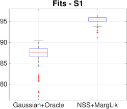
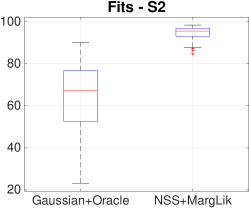
Figure 1: Boxplots of the 100 test set fits achieved in the two scenaria by (1) equipped with the Gaussian kernel (31) relying on the oracle to select the regressors space dimension (left boxplots) and by the new kernel NSS (34) with all the hyperparameters tuned via marginal likelihood optimization (right boxplots).

The two left boxplots in Fig. 1 report the prediction fits achieved by this procedure applied to identify the first (top) and the second (bottom) system. Even if the Gaussian kernel is equipped with the oracle, its performance is satisfactory only in the (S1) scenario while the capability of predicting outputs in the (S2) case is poor during many runs. In place of the marginal likelihood, a cross-validation strategy has been also used for tuning $(\eta,\gamma)$, obtaining results similar to those here displayed.
During the Monte Carlo, even when the number of impulse response coefficients $\theta_{k}$ different from zero is quite large, we have noticed that a relatively small value for $m$ is frequently chosen, i.e. the oracle tends to use few past input values $(u_{t-1},u_{t-2},\ldots)$ to predict $y_{t}$. This indicates that the Gaussian kernel structure induces the oracle to introduce a significant bias to guard the estimator’s variance.
Now, we show that in this example model complexity can be better controlled avoiding the difficult and computationally expensive choice of discrete orders. In particular, we set $m=\infty$ and use the new NSS kernel (34). For tuning the NSS hyperparameter vector $(\alpha,\eta,\gamma)$, no oracle having access to the test set is employed but just a single continuous optimization of the marginal likelihood that uses only the identification data. The fits achieved by NSS after the two Monte Carlo studies are in the right boxplots of the two figures above: in both the cases the new estimator behaves very nicely.

5 Consistency of regularization networks for system identification

5.1 The regression function

In what follows, the system input $u$ is a stationary stochastic process over $\mathbb{Z}$ in discrete-time or $\mathbb{R}$ in continuous-time. The distribution of $u$ induces on $\mathcal{X}$ the (Borel non degenerate) probability measure $\mu_{x}$, from which the input locations $x_{i}$ are drawn. In view of their dependence on $u$, the $x_{i}$ are in general correlated each other and unbounded, e.g. for Gaussian $u$ no bounded set contains $x_{i}$ with probability one. Such peculiarities, inherited by the system identification setting, already violate the data generation assumptions routinely adopted in machine learning.
The identification data $\{x_{i},y_{i}\}_{i=1}^{\infty}$ are assumed to be a stationary stochastic process. In particular, each couple $(x,y)$ has joint probability measure $\mu_{yx}(y,x)=\mu_{y|x}(y|x)\mu_{x}(x)$ where $\mu_{y|x}$ is the probability measure of the output $y$ conditional on a particular input location $x$.
Given a function (dynamic system) $f$, the least squares error associated to $f$ is

$$\mathcal{E}(y-f(x))^{2}=\int_{\mathcal{X}\times\mathbb{R}}\ \left(y-f(x)\right)^{2}d\mu_{yx}(y,x).$$ (36)

The following result is well known and characterizes the minimizer of (36) which goes under the name of regression function in machine learning.

Theorem 13 (The regression function).

We have

$$f_{\rho}=\operatorname*{arg\,min}_{f}\ \mathcal{E}(y-f(x))^{2},$$

where $f_{\rho}$ is the regression function defined for any $x\in\mathcal{X}$ by

$$f_{\rho}(x)=\int_{\mathbb{R}}y\ d\mu_{y|x}(y|x).$$ (37)

In our system identification context, $f_{\rho}$ is the dynamic system associated to the optimal predictor that minimizes the expected quadratic loss on a new output drawn from $\mu_{yx}$.

5.2 Consistency of regularization networks for system identification

Consider a scenario where $\mu_{y|x}$ (and possibly also $\mu_{x}$) is unknown and only $N$ samples $\{x_{i},y_{i}\}_{i=1}^{N}$ from $\mu_{yx}$ are available. We study the convergence of the RN in (1) to the optimal predictor $f_{\rho}$ as $N\rightarrow\infty$ under the input-induced norm

$$\|f\|_{x}^{2}=\int_{\mathcal{X}}\ f^{2}(x)d\mu_{x}(x).$$

This is the norm in the classical Lebesgue space $\mathcal{L}_{2}^{\mu_{x}}$ already introduced at the end of Section 2.
We assume that the reproducing kernel of $\mathcal{H}$ admits the expansion

$$\mathcal{K}(x,a)=\sum_{i=1}^{\infty}\ \zeta_{i}\rho_{i}(x)\rho_{i}(a),\ \ \zeta_{i}>0\ \forall i,$$

with $\zeta_{i}$ and $\rho_{i}$ defined via (10) and the probability measure $\mu_{x}$.
Exploiting the regression function, the measurements process can be written as

$$y_{i}=f_{\rho}(x_{i})+e_{i},$$ (38)

where the errors $e_{i}$ are zero-mean and identically distributed. They can be correlated each other and also with the input locations $x_{i}$. Given any $f\in\mathcal{H}$ and the $\ell$-th kernel eigenfunction $\rho_{\ell}$, we define the random variables $\{v_{\ell i}\}_{i\in\mathcal{Z}}$ by combining $f$, $\rho_{\ell}$ and the errors $e_{i}$ defined by (38) as follows

$$v_{\ell i}=\left(f(x_{i})+e_{i}\right)\rho_{\ell}(x_{i}).$$ (39)

Let $\mathcal{H}$ be stable so that the $\{v_{\ell i}\}$ form a stationary process. In particular, note that each $v_{\ell i}$ is the product of the outputs from two stable systems: the first one, $f(x_{i})+e_{i}$, is corrupted by noise while the second one, $\rho_{\ell}(x_{i})$, is noiseless.
Now, by summing up over $\ell$ the cross covariances of lag $k$ using kernel eigenvalues $\zeta_{\ell}$ as weights one obtains

$$c_{k}:=\sum_{\ell=1}^{\infty}\ \zeta_{\ell}Cov\left(v_{\ell i},v_{\ell,i+k}\right)$$ (40)

where $Cov(\cdot,\cdot)$ is the covariance operator. The next proposition shows that summability of the $c_{k}$ is key for consistency.

Proposition 14.

(RN consistency in system identification) Let $\mathcal{H}$ be the RKHS with kernel

$$\mathcal{K}(x,a)=\sum_{i=1}^{\infty}\ \zeta_{i}\rho_{i}(x)\rho_{i}(a),\ \ \zeta_{i}>0\ \forall i,$$ (41)

where $(\zeta_{i},\rho_{i})$ are the eigenvalues/eigenfunctions pairs defined by (10) under the probability measure $\mu_{x}$. Assume that, for any $r>0$ and $f$ s.t. $\|f\|_{\mathcal{H}}\leq r$, there exists a constant $C_{r}$ such that

$$\sum_{k=0}^{\infty}\ |c_{k}|<C_{r}<\infty,$$ (42)

with $c_{k}$ defined in (40). Let also

$$\gamma\propto\frac{1}{N^{\alpha}},$$ (43)

where $\alpha$ is any scalar in $(0,\frac{1}{2})$. Then, if $f_{\rho}\in\mathcal{H}$ and $\hat{g}_{N}$ is the RN in (1), as $N\rightarrow\infty$ one has

$$\|\hat{g}_{N}-f_{\rho}\|_{x}\longrightarrow_{p}0,$$ (44)

where $\longrightarrow_{p}$ denotes convergence in probability.

The fact that $\sum_{\ell=1}^{\infty}\ |\zeta_{\ell}|<\infty$ is already an indication that (42) is not so hard to be satisfied. Indeed, to the best of our knowledge, (42) is the weakest RKHS condition currently available which guarantees RN consistency. In fact, previous works, like [83, 69], beyond considering only noises with densities of compact support use mixing conditions (which rule out infinite memory systems) with fast mixing coefficients decay. These assumptions largely imply (42) as it can e.g. be deduced by Lemma 2.2 in [21].

From (40) one can see that (42) essentially reduces to studying summability of the covariances of the $v_{\ell i}=\left(f(x_{i})+e_{i}\right)\rho_{\ell}(x_{i})$. In particular, the covariance of such product sequences depends on the first four moments of the component sequences, see eq. 3.1 in [79]. The stability of $\mathcal{H}$ is thus crucial to ensure the existence of the moments of the $v_{\ell i}$. This is e.g. connected with the use of kernels like (19,22,34) where the influence of past input locations on the output decays exponentially to zero as time progresses.

The relevance and usefulness of (42) further emerges if more specific experimental conditions are considered. An example is given below by specializing Proposition 14 to the continuous-time linear setting. Here, the aim is to reconstruct the continuous-time impulse response of a linear system fed with a stationary input process from a sampled and noisy version of the output. Below, one can e.g. think of the sampling instants as $t_{i}=i\Delta+\delta_{i}$ where $\delta_{i}$ are identically distributed random variables with support on $[0,\Delta]$. Then, it is shown that, for Gaussian $u$, a weak condition on the input covariance’s decay rate already guarantees consistency. This outcome can also be seen as a non trivial extension to the dynamic context of studies on functional linear regression like e.g. that illustrated in [81] under independent data assumptions.

Proposition 15.

(RN consistency in continuous-time linear system identification) Let $\mathcal{H}$ be the RKHS with kernel $\mathcal{K}$ defined by the continuous-time stable spline kernel $K(t,s)=e^{-\beta\max(t,s)}$ with support restricted to any compact set of $\mathbb{R}_{+}\times\mathbb{R}_{+}$. Assume that

• the regression function $f_{\rho}$ is a continuous-time and time-invariant linear system with impulse response $\theta$ satisfying $\int\ \dot{\theta}^{2}(t)dt<\infty$;

• the system input $u$ is a stationary Gaussian process with $Cov(u(t+\tau),u(t))$ decaying to zero as $1/\tau^{1+\delta}$ for $\delta>0$;

• the errors $e_{i}$ in (38) are white, independent of the system input.

Then, letting $\gamma$ satisfy (43), the RN in (1) is consistent, i.e.

$$\|\hat{g}_{N}-f_{\rho}\|_{x}\longrightarrow_{p}0.$$ (45)

Remark 16 (Convergence to the true impulse response).

The optimal predictor $f_{\rho}$ is a dynamic system, unique as map $\mathcal{X}\rightarrow\mathbb{R}$. However, considering e.g. the linear scenario in Proposition 15, such functional can be associated to different impulse responses (as illustrated in Section 3.3 by discussing the relationship between the space $\mathcal{H}$ of linear dynamic systems and the space $\mathcal{I}$ of impulse responses). Convergence to $\theta$ can be guaranteed under persistently exciting conditions related to $u$ and the sampling instants $t_{i}$ [40]. One can then wonder which kind of impulse response estimate is obtained if such conditions are not satisfied. The answer is obtained by [53][Theorem 3 on p. 371] which reveals that the impulse response estimate (24) associated to $\hat{g}^{N}$ coincides with (15). Thus, among all the possible impulse responses defining the optimal predictor $f_{\rho}$, the estimator (24) will asymptotically privilege that of minimum norm in $\mathcal{I}$.

6 Conclusions

We have introduced a new look at system identification in a RKHS framework. Our approach uses RKHSs whose elements are functionals associated to dynamic systems. This perspective establishes a solid link between system identification and machine learning, with focus on the problem of learning from examples.
Such framework has led to simple derivations of RKHSs stability conditions in both linear and nonlinear scenarios. It has been also shown that stable spline kernels can be used as basic building blocks to define other models for nonlinear system identification.
In the last part of the paper, RN convergence to the optimal predictor has been proved under assumptions tailored to system identification, also pointing out the link between consistency and RKHS stability. This general treatment will hopefully pave the way for an even more fruitful interplay between RKHS theory and regularized system identification.

Appendix

Proof of Proposition 14

We start reporting three useful lemmas instrumental to the main proof. First, define

$$\hat{f}=\arg\min_{f\in\mathcal{H}}\|f-f_{\rho}\|^{2}_{x}+\gamma\|f\|^{2}_{\mathcal{H}}$$ (46)

and

$$\eta_{i}(\cdot)=\left[y_{i}-\hat{f}(x_{i})\right]\mathcal{K}(x_{i},\cdot).$$ (47)

In addition, the notation $S_{x}:\mathcal{H}\rightarrow\mathbb{R}^{N}$ is the sampling operator defined by $S_{x}f=[f(x_{1})\ldots f(x_{n})]$ while $S_{x}^{*}$ is its adjoint given by

$$S_{x}^{*}c=\sum_{i=1}^{N}\ c_{i}\mathcal{K}_{x_{i}}\quad\forall\ c\in\mathbb{R}^{N}.$$ (48)

The first lemma below involves the definitions of $\eta_{i},\hat{f},S_{x}$ and $S_{x}^{*}$ given above. It is derived from [66] and Proposition 1 in [65].

Lemma 17.

It holds that

$$\mathcal{E}\eta_{i}=\gamma\hat{f}.$$ (49)

Furthermore, if $v\in\mathcal{H}$ and $f$ satisfies

$$\left(\frac{S_{x}^{*}S_{x}}{N}+\gamma I\right)f=v,$$

where $I$ denotes the identity operator, one has

$$\|f\|_{\mathcal{H}}\leq\frac{1}{\gamma}\|v\|_{\mathcal{H}}.$$ (50)

The second lemma states a bound between the expected RKHS distance between $\hat{g}_{N}$ and $\hat{f}$.

Lemma 18.

Let $r=2\|f_{\rho}\|_{\mathcal{H}}$. Then, for any $\gamma>0$ one has

$$\mathcal{E}\mathcal{\|}\hat{g}_{N}-\hat{f}\|_{x}\leq\frac{1}{\gamma}\sqrt{\max\left(1,\max_{i}\ \zeta_{i}\right)}\sqrt{\frac{2C_{r}}{N}}.$$ (51)

Proof: It comes from the representer theorem and (48) that

$$\hat{g}_{N}=S_{x}^{*}\left(\mathbf{K}+N\gamma I_{N}\right)^{-1}Y.$$

Then, we have

$$\left(\frac{S_{x}^{*}S_{x}}{N}+\gamma I\right)\hat{g}_{N}$$

$$= \frac{S_{x}^{*}}{N}\left(\mathbf{K}\left(\mathbf{K}+N\gamma I_{N}\right)^{-1}+N\gamma\left(\mathbf{K}+N\gamma I_{N}\right)^{-1}\right)Y$$

$$= \frac{S_{x}^{*}}{N}Y.$$

Hence, one has

$$\hat{g}_{N}-\hat{f} = \left(\frac{S_{x}^{*}S_{x}}{N}+\gamma I\right)^{-1}\left(\frac{S_{x}^{*}Y}{N}-\frac{S_{x}^{*}S_{x}\hat{f}}{N}-\gamma\hat{f}\right)$$

$$= \left(\frac{S_{x}^{*}S_{x}}{N}+\gamma I\right)^{-1}\frac{1}{N}\sum_{i=1}^{N}\left(\eta_{i}-\mathcal{E}[\eta_{i}]\right),$$

where we used the equality $S_{x}^{*}Y-S_{x}^{*}S_{x}\hat{f}=\sum_{i=1}^{N}\eta_{i}$ and (49). Using (50) in Lemma 17, we then obtain

$$\|\hat{g}_{N}-\hat{f}\|_{\mathcal{H}}\leq\frac{1}{\gamma}\left\|\frac{1}{N}\sum_{i=1}^{N}\left(\eta_{i}-\mathcal{E}[\eta_{i}]\right)\right\|_{\mathcal{H}}.$$ (52)

Now, let $f:=f_{\rho}-\hat{f}$. With the $e_{i}$ defined in (38), we can write

$$\eta_{i}(\cdot)-\mathcal{E}\eta_{i}(\cdot)$$

$$= \left[f(x_{i})+e_{i}\right]\mathcal{K}(x_{i},\cdot)-\mathcal{E}\left[f(x_{i})+e_{i}\right]\mathcal{K}(x_{i},\cdot)$$

$$= \sum_{\ell=1}^{\infty}\zeta_{\ell}\left[(f(x_{i})+e_{i})\rho_{\ell}(x_{i})-\mathcal{E}(f(x_{i})+e_{i})\rho_{\ell}(x_{i})\right]\rho_{\ell}(\cdot)$$

$$= \sum_{\ell=1}^{\infty}\zeta_{\ell}\left[v_{\ell i}-m_{\ell}\right]\rho_{\ell}(\cdot)$$

where $v_{\ell i}=\left(f(x_{i})+e_{i}\right)\rho_{\ell}(x_{i})$ and $m_{\ell}=\mathcal{E}v_{\ell i}$. Now, the structure of the RKHS norm outlined in (9) allows us to write

$$\langle\eta_{i}(\cdot)-\mathcal{E}\eta_{i},\eta_{j}(\cdot)-\mathcal{E}\eta_{j}\rangle_{\mathcal{H}}$$

$$= \langle\sum_{\ell=1}^{\infty}\zeta_{\ell}\left(v_{\ell i}-m_{\ell}\right)\rho_{\ell}(\cdot),\sum_{\ell=1}^{\infty}\zeta_{\ell}\left(v_{\ell j}-m_{\ell}\right)\rho_{\ell}(\cdot)\rangle_{\mathcal{H}}$$

$$= \sum_{\ell=1}^{\infty}\zeta_{\ell}\left(v_{\ell i}-m_{\ell}\right)\left(v_{\ell j}-m_{\ell}\right).$$

So, using definition (40)

$$\mathcal{E}\langle\eta_{i}-\mathcal{E}\eta_{i},\eta_{j}-\mathcal{E}\eta_{j}\rangle_{\mathcal{H}}$$

$$= \sum_{\ell=1}^{\infty}\zeta_{\ell}Cov\left(v_{\ell i},v_{\ell,j}\right)$$

$$= c_{|i-j|}.$$

Comparing the values of the objective in (46) at the optimum $\hat{f}$ and at $f_{\rho}$, one finds $\|\hat{f}\|_{\mathcal{H}}\leq\|f_{\rho}\|_{\mathcal{H}}$ so that

$$\|f_{\rho}-\hat{f}\|_{\mathcal{H}}=\|f\|_{\mathcal{H}}\leq 2\|f_{\rho}\|_{\mathcal{H}}.$$

This, combined with (42), implies that for any $\gamma>0$

$$\sum_{k=0}^{\infty}\ |c_{k}|<C_{r}<\infty,\quad r=2\|f_{\rho}\|_{\mathcal{H}}.$$

Hence, we obtain

$$\mathcal{E}\left[\left\|\frac{1}{N}\sum_{i=1}^{N}\left(\eta_{i}-\mathcal{E}[\eta_{i}]\right)\right\|_{\mathcal{H}}^{2}\right]$$

$$\qquad\leq\frac{1}{N^{2}}\sum_{i=1}^{N}\sum_{j=1}^{N}|c_{|i-j|}|\leq\frac{2C_{r}}{N}.$$

Now, recall that, if $f=\sum_{i=1}^{\infty}a_{i}\rho_{i}$, then $\|f\|_{\mathcal{H}}^{2}=\sum_{i=1}^{\infty}\frac{a_{i}^{2}}{\zeta_{i}}$ while $\|f\|_{x}^{2}=\sum_{i=1}^{\infty}a_{i}^{2}$. Thus, for any $f\in\mathcal{H}$, one has

$$\|f\|^{2}_{x}\leq\max\left(1,\max_{i}\ \zeta_{i}\right)\|f\|^{2}_{\mathcal{H}}.$$

The use of Jensen’s inequality and (52) then completes the proof.

$\blacksquare$

Now, we need to set up some additional notation. Following [65, 66], given the integral operator

$$L_{\mathcal{K}}[\rho_{i}]:=\int_{\mathcal{X}}\mathcal{K}(\cdot,u)\rho_{i}(u)d\mu_{x}(u)=\zeta_{i}\rho_{i},$$

for $r>0$ we define

$$L_{\mathcal{K}}^{-r}[f]=\sum_{i=1}^{\infty}\frac{c_{i}}{\zeta_{i}^{r}}\rho_{i}.$$

The third lemma reported below contains the inequality (53) which was also derived in [65] assuming a compact input space. However, the bound holds just assuming the validity of the kernel expansion (41). To see this, recalling Theorem 5, first note that $L_{\mathcal{K}}^{-r}f_{\rho}\in\mathcal{L}_{2}^{\mu_{x}}$ for any $0\leq r\leq 1/2$. So, there exists $g\in\mathcal{L}_{2}^{\mu_{x}}$, say $g=\sum_{i=1}^{\infty}d_{i}\rho_{i}$, such that $f_{\rho}=\sum_{i=1}^{\infty}\zeta_{i}^{r}d_{i}\rho_{i}$. After simple computations, one obtains $\hat{f}-f_{\rho}=-\sum_{i=1}^{\infty}\frac{\gamma}{\zeta_{i}+\gamma}\zeta_{i}^{r}d_{i}\rho_{i}$ and the same manipulations contained in the proof of Theorem 4 in [65][p. 295] lead to the following result.

Lemma 19.

For any $0<r\leq 1/2$, one has

$$\|\hat{f}-f_{\rho}\|_{x}\leq\gamma^{\ r}\|L_{\mathcal{K}}^{-r}f_{\rho}\|_{x}$$ (53)

Combining (51) and (53), for any $0<r\leq 1/2$ it holds that

$$\mathcal{E}\|\hat{g}_{N}-f_{\rho}\|_{x}\leq\gamma^{\ r}\|L_{\mathcal{K}}^{-r}f_{\rho}\|_{x}+\frac{1}{\gamma}\sqrt{\max\left(1,\max_{i}\ \zeta_{i}\right)}\sqrt{\frac{2C_{r}}{N}}.$$ (54)

Hence, when $\gamma$ is chosen according to (43), $\mathcal{E}\|\hat{g}_{N}-f_{\rho}\|_{x}$ converges to zero as $N$ grows to $\infty$. Using the Markov inequality, (44) is finally obtained.

Proof of Proposition 15

Let $\mathcal{I}$ be the space of impulse responses with compact support e.g. on $[0,T]$ induced by the stable spline kernel $K$. Then, it comes from [49] that $\|\theta\|_{\mathcal{I}}^{2}\propto\int_{0}^{T}\dot{\theta}^{2}(t)e^{\beta t}dt$. So, finite energy of the first derivative of $\theta$ ensures that the optimal predictor $f_{\rho}$ belongs the RKHS $\mathcal{H}$ defined by the linear kernel $\mathcal{K}$ induced by $K$.
Now, we have just to prove that condition (42) holds. Recall that the $c_{k}$ are invariant w.r.t. the particular kernel expansion of $\mathcal{K}$ adopted. For the stable spline kernel $K$ we choose the expansion $K(t,\tau)=\sum_{\ell=1}^{\infty}\zeta_{\ell}\psi_{\ell}(t)\psi_{\ell}(\tau)$ derived in [49] where

$$\psi_{\ell}(t)=\sqrt{2}\sin\left(\frac{e^{-\beta s}}{\sqrt{\zeta_{\ell}}}\right),\quad\zeta_{\ell}=\frac{1}{(\ell\pi-\pi/2)^{2}}.$$

The eigenfunctions thus satify

$$|\psi_{\ell}(t)|<\sqrt{2}\ \ \forall(\ell,t).$$ (55)

Now, let $f$ be any dynamic system satisfying $\|f\|_{\mathcal{H}}\leq r$ and let $\theta$ be the associated impulse response of minimum norm living in $\mathcal{I}.$ From the arguments discussed in section 3.3 one then has $\|\theta\|_{\mathcal{I}}\leq r$. It then holds that

$$|\theta(t)|=|\langle\theta,K_{t}\rangle_{\mathcal{I}}|\leq r\sqrt{K(t,t)}\implies\max_{t\in[0,T]}|\theta(t)|\leq A_{r}<\infty$$ (56)

with $A_{r}$ independent of the particular $f$ chosen inside the ball of radius $r$ of $\mathcal{H}$.
Without loss of generality, the input $u$ is now assumed zero-mean so that the $f(x_{i})$ and $\rho_{\ell}(x_{i})$ become zero-mean Gaussian processes. Using eq. 3.2 in [79], for $k>1$ one obtains

$$Cov\left(v_{\ell i},v_{\ell,i+k}\right) = Cov\left(f(x_{i})\rho_{\ell}(x_{i}),f(x_{i+k})\rho_{\ell}(x_{i+k})\right)$$

$$= Cov\left(f(x_{i}),f(x_{i+k})\right)Cov\left(\rho_{\ell}(x_{i}),\rho_{\ell}(x_{i+k})\right)$$

$$+ Cov\left(f(x_{i}),\rho_{\ell}(x_{i+k})\right)Cov\left(f(x_{i}),\rho_{\ell}(x_{i-k})\right).$$

(57)

Now, let $h$ be any of the four covariances in the r.h.s. of (57). Combining (55,56) and classical integral formulas for covariances computations, as e.g. reported in [47][p. 308-313], it is easy to obtain a constant $B_{r}$ independent of $\ell$ such that $|h(k)|\leq B_{r}/k^{1+\epsilon}$. Condition (42) thus holds true and this completes the proof.

References

- [1] H. Akaike. Smoothness priors and the distributed lag estimator. Technical report, Department of Statistics, Stanford University, 1979.
- [2] N. Alon, S. Ben-David, N. Cesa-Bianchi, and D. Haussler. Scale-sensitive dimensions, uniform convergence, and learnability. J. ACM, 44(4):615–631, 1997.
- [3] A. Aravkin, J.V. Burke, A. Chiuso, and G. Pillonetto. On the estimation of hyperparameters for empirical bayes estimators: Maximum marginal likelihood vs minimum mse. IFAC Proceedings Volumes, 45(16):125 – 130, 2012.
- [4] A. Aravkin, J.V. Burke, A. Chiuso, and G. Pillonetto. Convex vs non-convex estimators for regression and sparse estimation: the mean squared error properties of ard and glasso. Journal of Machine Learning Research, 15:217–252, 2014.
- [5] A.Y. Aravkin, B.M. Bell, J.V. Burke, and G. Pillonetto. The connection between Bayesian estimation of a Gaussian random field and RKHS. Neural Networks and Learning Systems, IEEE Transactions on, 26(7):1518–1524, 2015.
- [6] A. Argyriou and F. Dinuzzo. A unifying view of representer theorems. In Proceedings of the 31th International Conference on Machine Learning, volume 32, pages 748–756, 2014.
- [7] A. Argyriou, C.A. Micchelli, and M. Pontil. When is there a representer theorem? vector versus matrix regularizers. J. Mach. Learn. Res., 10:2507–2529, 2009.
- [8] N. Aronszajn. Theory of reproducing kernels. Trans. of the American Mathematical Society, 68:337–404, 1950.
- [9] E. Bai and Y. Liu. Recursive direct weight optimization in nonlinear system identification: a minimal probability approach. IEEE Trans. Automat. Contr., 52(7):1218–1231, 2007.
- [10] E. W. Bai. Non-parametric nonlinear system identification: An asymptotic minimum mean squared error estimator. IEEE Transactions on Automatic Control, 55(7):1615–1626, 2010.
- [11] B.M. Bell and G. Pillonetto. Estimating parameters and stochastic functions of one variable using nonlinear measurement models. Inverse Problems, 20(3):627, 2004.
- [12] S. Bergman. The Kernel Function and Conformal Mapping. Mathematical Surveys and Monographs, AMS, 1950.
- [13] M. Bertero. Linear inverse and ill-posed problems. Advances in Electronics and Electron Physics, 75:1–120, 1989.
- [14] M. Bertero, T. Poggio, and V. Torre. Ill-posed problems in early vision. In Proceedings of the IEEE, pages 869–889, 1988.
- [15] O. Bousquet and A. Elisseeff. Stability and generalization. J. Mach. Learn. Res., 2:499–526, 2002.
- [16] C. Carmeli, E. De Vito, and A. Toigo. Vector valued reproducing kernel Hilbert spaces of integrable functions and Mercer theorem. Analysis and Applications, 4:377–408, 2006.
- [17] V. Chandrasekaran, B. Recht, P.A. Parrilo, and A.S. Willsky. The convex geometry of linear inverse problems. Foundations of Computational Mathematics, 12(6):805–849, 2012.
- [18] T. Chen, H. Ohlsson, and L. Ljung. On the estimation of transfer functions, regularizations and Gaussian processes - revisited. Automatica, 48(8):1525–1535, 2012.
- [19] F. Cucker and S. Smale. On the mathematical foundations of learning. Bulletin of the American mathematical society, 39:1–49, 2001.
- [20] G. De Nicolao, G. Sparacino, and C. Cobelli. Nonparametric input estimation in physiological systems: problems, methods and case studies. Automatica, 33:851–870, 1997.
- [21] H. Dehling and W. Philipp. Almost sure invariance principles for weakly dependent vector-valued random variables. The Annals of Probability, 10(3):689–701, 1982.
- [22] F. Dinuzzo. Kernels for linear time invariant system identification. SIAM Journal on Control and Optimization, 53(5):3299–3317, 2015.
- [23] H. Drucker, C.J.C. Burges, L. Kaufman, A. Smola, and V. Vapnik. Support vector regression machines. In Advances in Neural Information Processing Systems, 1997.
- [24] T. Evgeniou and M. Pontil. On the dimension for regression in reproducing kernel Hilbert spaces. In Algorithmic Learning Theory, 10th International Conference, ALT ’99, Tokyo, Japan, December 1999, Proceedings, volume 1720 of Lecture Notes in Artificial Intelligence, pages 106–117. Springer, 1999.
- [25] T. Evgeniou, M. Pontil, and T. Poggio. Regularization networks and support vector machines. Advances in Computational Mathematics, 13:1–50, 2000.
- [26] M.O. Franz and B. Schölkopf. A unifying view of Wiener and volterra theory and polynomial kernel regression. Neural Computation, 18:3097–3118, 2006.
- [27] R. Frigola, F. Lindsten, T.B. Schon, and C.E. Rasmussen. Bayesian inference and learning in Gaussian process state-space models with particle mcmc. In Advances in Neural Information Processing Systems (NIPS), 2013.
- [28] R. Frigola and C.E. Rasmussen. Integrated pre-processing for Bayesian nonlinear system identification with Gaussian processes. In Proceedings of the 52nd Annual Conference on Decision and Control (CDC), 2013.
- [29] F. Girosi. An equivalence between sparse approximation and support vector machines. Technical report, Cambridge, MA, USA, 1997.
- [30] G.C. Goodwin, M. Gevers, and B. Ninness. Quantifying the error in estimated transfer functions with application to model order selection. IEEE Trans. on Automatic Control, 37(7):913–928, 1992.
- [31] C. Grossmann, C.N. Jones, and M. Morari. System identification via nuclear norm regularization for simulated moving bed processes from incomplete data sets. In Proceedings of the 48th IEEE Conference on Decision and Control (CDC), pages 4692–4697, 2009.
- [32] Z.C. Guo and D.X. Zhou. Concentration estimates for learning with unbounded sampling. Adv. Comput. Math., 38(1):207–223, 2013.
- [33] H. Hochstadt. Integral equations. John Wiley and Sons, 1973.
- [34] G. Kimeldorf and G. Wahba. A correspondence between bayesian estimation on stochastic processes and smoothing by splines. The Annals of Mathematical Statistics, 41(2):495–502, 1970.
- [35] G. Kimeldorf and G. Wahba. A correspondence between Bayesan estimation of stochastic processes and smoothing by splines. Ann. Math. Statist., 41(2):495–502, 1971.
- [36] G. Kitagawa and W. Gersch. Smoothness priors analysis of time series. Springer, 1996.
- [37] W. E. Leithead, E. Solak, and D. J. Leith. Direct identification of nonlinear structure using Gaussian process prior models. In Proceedings of European Control Conference (ECC 2003), 2003.
- [38] T. Lin, B.G. Horne, P. Tino, and C.L. Giles. Learning long-term dependencies in NARX recurrent neural networks. IEEE Trans. on Neural Networks, 7:1329 – 1338, 1996.
- [39] Z. Liu and L. Vandenberghe. Interior-point method for nuclear norm approximation with application to system identification. SIAM Journal on Matrix Analysis and Applications, 31(3):1235–1256, 2009.
- [40] L. Ljung. System Identification - Theory for the User. Prentice-Hall, Upper Saddle River, N.J., 2nd edition, 1999.
- [41] L. Ljung, G.C. Goodwin, and J. C. Ag ero. Stochastic embedding revisited: A modern interpretation. In 53rd IEEE Conference on Decision and Control, pages 3340–3345, 2014.
- [42] M.N. Lukic and J.H. Beder. Stochastic processes with sample paths in reproducing kernel Hilbert spaces. Trans. Amer. Math. Soc., 353:3945–3969, 2001.
- [43] J. S. Maritz and T. Lwin. Empirical Bayes Method. Chapman and Hall, 1989.
- [44] J. Mercer. Functions of positive and negative type and their connection with the theory of integral equations. Philos. Trans. Roy. Soc. London, 209(3):415–446, 1909.
- [45] K. Mohan and M. Fazel. Reweighted nuclear norm minimization with application to system identification. In American Control Conference (ACC), pages 2953–2959, 2010.
- [46] S. Mukherjee, P. Niyogi, T. Poggio, and R. Rifkin. Learning theory: stability is sufficient for generalization and necessary and sufficient for consistency of empirical risk minimization. Advances in Computational Mathematics, 25(1):161–193, 2006.
- [47] A. Papoulis. Probability, Random Variables and Stochastic Processes. Mc Graw-Hill, 1991.
- [48] G. Pillonetto, T. Chen, A. Chiuso, G. De Nicolao, and L. Ljung. Regularized linear system identification using atomic, nuclear and kernel-based norms: The role of the stability constraint. Automatica, 69:137 – 149, 2016.
- [49] G. Pillonetto, A. Chiuso, and G. De Nicolao. Regularized estimation of sums of exponentials in spaces generated by stable spline kernels. In Proceedings of the IEEE American Cont. Conf., Baltimora, USA, 2010.
- [50] G. Pillonetto, A. Chiuso, and G. De Nicolao. Prediction error identification of linear systems: a nonparametric Gaussian regression approach. Automatica, 47(2):291–305, 2011.
- [51] G. Pillonetto, A. Chiuso, and Minh Ha Quang. A new kernel-based approach for nonlinear system identification. IEEE Trans. on Automatic Control, 56(12):2825–2840, 2011.
- [52] G. Pillonetto and G. De Nicolao. A new kernel-based approach for linear system identification. Automatica, 46(1):81–93, 2010.
- [53] G. Pillonetto, F. Dinuzzo, T. Chen, G. De Nicolao, and L. Ljung. Kernel methods in system identification, machine learning and function estimation: a survey. Automatica, 50(3):657–682, 2014.
- [54] T. Poggio and F. Girosi. Networks for approximation and learning. In Proceedings of the IEEE, volume 78, pages 1481–1497, 1990.
- [55] T. Poggio, R. Rifkin, S. Mukherjee, and P. Niyogi. General conditions for predictivity in learning theory. Nature, 428(6981):419–422, 2004.
- [56] Tomaso Poggio and Christian R. Shelton. Machine learning, machine vision, and the brain. AI Magazine, 20(3):37–55, 1999.
- [57] C.E. Rasmussen and C.K.I. Williams. Gaussian Processes for Machine Learning. The MIT Press, 2006.
- [58] C.R. Rojas, R. Toth, and H. Hjalmarsson. Sparse estimation of polynomial and rational dynamical models. IEEE Transactions on Automatic Control, 59(11):2962–2977, 2014.
- [59] J. Roll, A. Nazin, and L. Ljung. Nonlinear system identification via direct weight optimization. Automatica, 41(3):475–490, 2005.
- [60] R.J. Schiller. A distributed lag estimator derived from smoothness priors. Economics Letters, 2(3):219 – 223, 1979.
- [61] B. Schölkopf, R. Herbrich, and A. J. Smola. A generalized representer theorem. Neural Networks and Computational Learning Theory, 81:416–426, 2001.
- [62] B. Schölkopf and A. J. Smola. Learning with Kernels: Support Vector Machines, Regularization, Optimization, and Beyond. (Adaptive Computation and Machine Learning). MIT Press, 2001.
- [63] S. Shun-Feng and F.Y.P. Yang. On the dynamical modeling with neural fuzzy networks. IEEE Transactions on Neural Networks, 13:1548 – 1553, 2002.
- [64] J. Sjöberg, Q. Zhang, L. Ljung, B. Delyon A. Benveniste, P. Glorennec, H. Hjalmarsson, and A. Juditsky. Nonlinear black-box modeling in system identification: A unified overview. Automatica, 31(12):1691–1724, December 1995.
- [65] S. Smale and D.X. Zhou. Shannon sampling II: connections to learning theory. Appl. Comput. Harmon. Anal., 19:285–302, 2005.
- [66] S. Smale and D.X. Zhou. Learning theory estimates via integral operators and their approximations. Constructive Approximation, 26:153–172, 2007.
- [67] W. Spinelli, L. Piroddi, and M. Lovera. On the role of prefiltering in nonlinear system identification. IEEE Transactions on Automatic Control, 50(10):1597–1602, 2005.
- [68] I. Steinwart, D. Hush, and C. Scovel. Learning from dependent observations. Journal of Multivariate Analysis, 100(1):175 – 194, 2009.
- [69] H. Sun and Q. Wu. Regularized least square regression with dependent samples. Advances in computational mathematics, 32(2):175 – 189, 2010.
- [70] Hongwei Sun. Mercer theorem for RKHS on noncompact sets. J. Complexity, 21(3):337–349, 2005.
- [71] J.A.K. Suykens, C. Alzate, and K. Pelckmans. Primal and dual model representations in kernel-based learning. Statist. Surv., 4:148–183, 2010.
- [72] J.A.K. Suykens, T. Van Gestel, J. De Brabanter, B. De Moor, and J. Vandewalle. Least Squares Support Vector Machines. World Scientific, Singapore, 2002.
- [73] J.A.K. Suykens, T. Van Gestel, J. De Brabanter, B. De Moor, and J. Vandewalle. Least Squares Support Vector Machines. World Scientific, Singapore, 2002.
- [74] A.N. Tikhonov and V.Y. Arsenin. Solutions of Ill-Posed Problems. Washington, D.C.: Winston/Wiley, 1977.
- [75] V. Vapnik. Statistical Learning Theory. Wiley, New York, NY, USA, 1998.
- [76] G. Wahba. Spline models for observational data. SIAM, Philadelphia, 1990.
- [77] Grace Wahba. Practical approximate solutions to linear operator equations when the data are noisy. SIAM Journal on Numerical Analysis, 14(4):651–667, 1977.
- [78] C. Wang and D.X. Zhou. Optimal learning rates for least squares regularized regression with unbounded sampling. Journal of Complexity, 27(1):55 – 67, 2011.
- [79] W.E. Wecker. A note on the time series which is the product of two stationary time series. Stochastic Processes and their Applications, 8(2):153 – 157, 1978.
- [80] Q. Wu, Y Ying, and D.X. Zhou. Learning rates of least-square regularized regression. Foundations of Computational Mathematics, 6:171–192, 2006.
- [81] M. Yuan and T. Tony Cai. A reproducing kernel Hilbert space approach to functional linear regression. Annals of Statistics, 38:3412–3444, 2010.
- [82] W. Zhao, H.F. Chen, E. Bai, and K. Li. Kernel-based local order estimation of nonlinear nonparametric systems. Automatica, 51:243–254, 2015.
- [83] B. Zou, L. Li, and Z. Xu. The generalization performance of erm algorithm with strongly mixing observations. Machine Learning, 75:275–295, 2009.