Annotations on the virtual element method
for second-order elliptic problems

​​1.  Introduction

1.1. This document contains working annotations on the Virtual Element Method (VEM) for the approximate solution of diffusion problems with variable coefficients. To read this document you are assumed to have familiarity with concepts from the numerical discretization of Partial Differential Equations (PDEs) and, in particular, the Finite Element Method (FEM). This document is not an introduction to the FEM, for which many textbooks (also free on the internet) are available. Eventually, this document is intended to evolve into a tutorial introduction to the VEM (but this is really a long-term goal).

1.1.1. To ease the exposition, we will refer to the Laplace problem and consider the conforming method for the primal form in two space dimensions.

1.2. Acronyms used in this document:

• FEM = Finite Element Method

• VEM = Virtual Element Method

• MFD = Mimetic Finite Difference method

• PFEM = Polygonal Finite Element Method

• PDE = Partial Differential Equation

1.3. The Virtual Element Method is a kind of Finite Element Methods where trial and test functions are the solutions of a PDE problem inside each element.

1.3.1. A naive approach to implement the VEM would consists in solving each local PDE problem to compute the trial and test functions at least approximately where needed (for example, at the quadrature nodes of the element).

1.4. The key point in the VEM approach is that some elliptic and $L^{2}$ polynomial projections of functions and gradients of functions that belong to the finite element space are computable exactly using only their degrees of freedom. So, the VEM strategy is to substitute test and trial functions in the bilinear forms and linear functionals of the variational formulations with their polynomial projections whenever these latters are computable. In fact, the value of such bilinear forms is exact whenever at least one of the entries is a polynomial function of a given degree. We refer to this exactness property as the polynomial consistency or, simply, the consistency of the method. This strategy leads to an underdetermined formulation (the global stiffness matrix is rank deficient). In the VEM we fix this issue by adding a stabilization term to the bilinear form. Stabilization terms are required not to upset the exactness property for polynomials and to scale properly with respect to the mesh size and the problem coefficients.

1.4.1. The low-order setting for polygonal cells (in 2D) and polyhedral cells (in 3D) can be obtained as a straightforward generalization of the FEM. The high-order setting deserves special care in the treatment of variable coefficients in order not to loose the optimality of the discretization and in the 3D formulation.

1.5. The shape functions are virtual in the sense that we never compute them explicitly (not even approximately) inside the elements. Note that the polynomial projection of the approximate solution is readily available from the degrees of freedom and we can use it as the numerical solution.

1.6. The major advantage offered by the VEM is in the great flexibility in admitting unstructured polygonal and polyhedral meshes.

1.7. The VEM can be seen as an evolution of the MFD method. Background material (and a few historical notes) will be given in the final section of this document.

​​2.  Meshes

2.1. Meshes with polygonal & polyhedral cells.

The VEM inherits the great flexibility of the MFD method and is suitable to approximate PDE problems on unstructured meshes of cells with very general geometric shapes. The mesh flexibility is a major feature of this kind of discretization, as we often need that computational meshes should be easily adaptable to:

• the geometric characteristics of the domain;

• the solution.

2.1.1. Examples of 2D meshes used in academic problems are given in Figure 1.

Figure 1: Convex and non-convex cells; highly deformed cells; local adaptive refinements (AMR, hanging nodes).

2.1.2. Examples of 3D meshes used in academic problems are given in Figure 2.

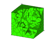
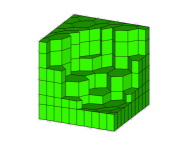
Figure 2: Random hexahedra; prysmatic meshes; local adaptive refinements (AMR, hanging nodes).

​​3.  Formulations

To introduce the basic ideas of the virtual element method, we first consider the case of the Laplace equation. Let $\Omega\subset\mathbbm{R}^{d}$ ($d=2$) be a polygonal domain with boundary $\Gamma$. We use standard notation on Sobolev (and Hilbert) spaces, norms, and semi-norms. Hereafter, $H^{1}_{g}(\Omega)$ denotes the affine Sobolev space of functions in $L^{2}(\Omega)$ with first derivatives in $L^{2}(\Omega)$, and boundary trace equal to $g$; $H^{1}_{0}(\Omega)$ is the subspace of $H^{1}(\Omega)$ corresponding to $g=0$. Also, we assume that $f\in L^{2}(\Omega)$ and $g\in H^{\frac{1}{2}}(\Gamma)$.

3.1. Differential formulation. Find $u\in H^{1}(\Omega)$ such that:

$$-\Delta u =f\phantom{g~{}}\textrm{in~{}~{}}\Omega,$$

$$u =g\phantom{f~{}}\textrm{on~{}~{}}\Gamma.$$

3.2. Variational formulation. Find $u\in H^{1}_{g}(\Omega)$ such that:

$$\mathcal{A}\big{(}u,v\big{)}:=\int_{\Omega}\nabla u\cdot\nabla v\,dV=\int_{\Omega}fv\,dV=:\big{(}f,v\big{)}\qquad\forall v\in H^{1}_{0}(\Omega).$$

3.3. Finite element formulation. Find $u_{h}\in V_{h,g}\subset H^{1}_{g}(\Omega)$ such that:

$$\mathcal{A}\big{(}u_{h},v_{h}\big{)}:=\int_{\Omega}\nabla u_{h}\cdot\nabla v_{h}\,dV=\int_{\Omega}fv_{h}\,dV=:\big{(}f,v_{h}\big{)}\quad\forall v_{h}\in V_{h,0}\subset H^{1}_{0}(\Omega),$$

where $V_{h,g}$ and $V_{h,0}$ are finite dimensional affine and linear functional spaces, dubbed the finite element spaces (see Section 4 for the formal definition).

3.4. A short guide to a happy life (with VEM)

Let $\mathsf{P}$ be a cell of a mesh partitioning $\Omega_{h}$ of domain $\Omega$. The construction of the VEM follows these four logical steps.

• Define the functions of the virtual element space $V_{h}(\mathsf{P})$ as the solution of a PDE problem;

• Split the virtual element space as the direct sum of a the polynomial subspace $\mathbbm{P}_{m}(\mathsf{P})$ of the polynomials of degree up to $m$ and its complement:
  

  $V_{h}(\mathsf{P})$ = [polynomials] $\oplus$ [non-polynomials].

  At this point, it is natural to introduce the polynomial projection operator $\Pi_{m}^{\nabla}:V_{h}(\mathsf{P})\to\mathbbm{P}_{m}(\mathsf{P})$ and reformulate the splitting above as:

  $$V_{h}(\mathsf{P})=\Pi^{*}_{m}\big{(}V_{h}(\mathsf{P})\big{)}\oplus\big{(}1-\Pi^{*}_{m}\big{)}\big{(}V_{h}(\mathsf{P})\big{)}.$$

• Define the virtual element approximation of the local bilinear form as the sum of two terms, respectively related to the consistency and the stability of the method:

  $$\int_{\mathsf{P}}\nabla u_{h}\cdot\nabla v_{h}\,dV\approx\text{\big{[}CONSISTENCY\big{]}}+\text{\big{[}STABILITY\big{]}}=:\mathcal{A}_{h,\mathsf{P}}\big{(}u_{h},v_{h}\big{)}.$$

• Prove the convergence theorem:
  

  [CONSISTENCY] + [STABILITY] $\Rightarrow$ [CONVERGENCE]

​​4.  Extending the linear conforming FEM from triangles to polygonal cells

4.1. The linear conforming Galerkin FEM on triangles. For every cell $\mathsf{P}$, we define the local finite element space as:

$$V_{h,\mathsf{P}}:=\Big{\{}v_{h}\in H^{1}(\mathsf{P})\,|\,v_{h}\in\mathbbm{P}_{1}(\mathsf{P})\Big{\}}.$$

Local spaces glue gracefully and yield the global finite element space:

$$V_{h}:=\big{\{}v_{h}\in H^{1}(\Omega)\,|\,v_{h}{}_{|\mathsf{P}}\in V_{h,\mathsf{P}}\,\,\forall\mathsf{P}\in\Omega_{h}\big{\}}\subset H^{1}(\Omega),$$

which is a conforming approximation of $H^{1}(\Omega)$.

4.1.1. We take into account the essential boundary conditions through the affine space

$$V_{h,g}:=\Big{\{}v_{h}\in V_{h,\mathsf{P}}\,|\,v_{h}{}_{|\Gamma}=g\Big{\}}$$

for the given boundary function $g\in H^{\frac{1}{2}}(\Gamma)$. We take $g=0$ in the definition above and consider the linear subspace $V_{h,0}\subset V_{h}$. The affine space $V_{h,g}$ and the linear space $V_{h,0}$ are respectively used for the trial and the test functions in the variational formulation.

4.1.2. The degrees of freedom of a virtual function $v_{h}\in V_{h}$ are the values at mesh vertices. Unisolvence can be proved and conformity of the global space is obvious.

4.2. An extension of the FEM to polygonal cells. We extend the FEM to polygonal meshes by redefining the local finite element space $V_{h,\mathsf{P}}$ on the polygonal cell $\mathsf{P}$. To this end, we require that

• the degrees of freedom of each function are its vertex values; therefore, the dimension of this functional space on cell $\mathsf{P}$ is equal to the number of vertices of the cell: $\text{dim}V_{h,\mathsf{P}}=N^{\mathcal{V}}_{\mathsf{P}}$;

• on triangles $V_{h,\mathsf{P}}$ must coincide with the linear Galerkin finite element space. This condition implies that $V_{h,\mathsf{P}}$ contains the linear polynomials $1$, $x$, $y$ and all their linear combinations;

• the local spaces $V_{h,\mathsf{P}}$ glue gracefully to give a conformal finite element space $V_{h}$ of functions globally defined on $\Omega$.

4.3. Shape functions on polygons. The construction of a set of shape functions defined on $\mathsf{P}$ and satisfying the requirements listed above is hard if we assume that $\mathsf{P}$ may have a general polygonal geometric shape. The challenge here is to define $V_{h,\mathsf{P}}$ by specifying the minimal information about its functions so that a computable variational formulation is possible. To achieve this task, we specify the behavior of the functions of $V_{h,\mathsf{P}}$ on $\partial\mathsf{P}$, for example by assuming that their trace on each polygonal boundary is a piecewise polynomial of an assigned degree. Then, we characterize them inside $\mathsf{P}$ in a very indirect way by assuming that they solve a partial differential equation.

4.4. The local finite element space on a generic polygonal cell. We define the local finite element space $V_{h,\mathsf{P}}$ as the span of a set of shape functions $\varphi_{i}\in H^{1}(P)$, which are associated with the cell vertices $\mathsf{v}_{i}$. A possible construction of these shape functions is given in the following three steps.

• For each vertex $\mathsf{v}_{i}$ consider the boundary function $\delta_{i}$ such that:

  • $\delta_{i}(\mathsf{v}_{j})=1$ if $i=j$, and $0$ otherwise;

  • $\delta_{i}$ is continuous on $\partial\mathsf{P}$ ;

  • $\delta_{i}$ is linear on each edge.

• Then, set $\quad{\varphi_{i}}{}_{|{\partial\mathsf{P}}}=\delta_{i}$;

• Finally, consider the function $\varphi_{i}$ that is the harmonic lifting of the function $\delta_{i}$ inside $\mathsf{P}$.

Eventually, we set:

$$V_{h,\mathsf{P}}:=\text{span}\{\varphi_{1},\dots,\phi_{N^{\mathcal{P}}}\}$$

4.5. The harmonic lifting.

We define the shape function $\varphi_{i}$ associated with vertex $i$ as the harmonic function on $\mathsf{P}$ having $\delta_{i}$ as trace on boundary $\partial\mathsf{P}$. Formally, $\varphi_{i}\in H^{1}(\mathsf{P})$ is the solution of the following elliptic problem:

$$-\Delta\varphi_{i} =0\phantom{\delta_{i}}\quad\text{in~{}}\mathsf{P},$$

$$\varphi_{i} =\delta_{i}\phantom{0}\quad\text{on~{}}\partial\mathsf{P}.$$

4.5.1. Properties of $\varphi_{i}$. Note that:

• the functions $\{\varphi_{i}\}$ are linearly independent (in the sense of the Gramian determinant);

• if $w_{h}\in V_{h,\mathsf{P}}$, then $w_{h}=\sum_{i=1}^{N^{\mathcal{P}}}w_{h}(\mathsf{v}_{i})\,\varphi_{i}$;

• linear polynomials belong to $V_{h,\mathsf{P}}$, i.e., $1,x,y\in V_{h,\mathsf{P}}$;

• the trace of each $\varphi_{i}$ on each edge of $\partial\mathsf{P}$ only depends on the vertex values of that edge. Consequently, the local spaces $V_{h,\mathsf{P}}$ glue together giving a conformal finite element space $V_{h}\subset H^{1}_{0}(\Omega)$.

4.5.2. Moreover, we can easily prove that:

• if $\mathsf{P}$ is a triangle, we recover the ${\mathbb{P}}_{1}$ Galerkin elements;

• if $\mathsf{P}$ is a square, we recover the ${\mathbb{Q}}_{1}$ bilinear elements.

4.6. The low-order local virtual element space. The low-order local virtual element space ($m=1$) is given by:

$$V_{h}^{1}(\mathsf{P})=\Big{\{}v_{h}\in H^{1}(\mathsf{P})\,:\, \Delta v_{h}=0,$$

$${v_{h}}_{|\mathsf{e}}\in\mathbbm{P}_{1}(\mathsf{e})\quad\forall\mathsf{e}\in\partial\mathsf{P},$$

$${v_{h}}_{|\partial\mathsf{P}}\in C^{0}(\partial\mathsf{P})\Big{\}}$$

4.6.1. Extension of the conforming virtual space to the high-order case. The high-order local VE space ($m\geq 2$) reads as:

$$V_{h}^{m}(\mathsf{P})=\Big{\{}v_{h}\in H^{1}(\mathsf{P})\,:\, \Delta v_{h}\in\mathbbm{P}_{m-2}(\mathsf{P}),$$

$${v_{h}}_{|\mathsf{e}}\in\mathbbm{P}_{m}(\mathsf{e})\quad\forall\mathsf{e}\in\partial\mathsf{P},$$

$${v_{h}}_{|\partial\mathsf{P}}\in C^{0}(\partial\mathsf{P})\Big{\}}$$

4.6.2. The local spaces glue gracefully to provide a conforming approximation of $H^{1}(\Omega)$. A natural way to guarantee the last property in the previous definitions, i.e., ${v_{h}}_{|\partial\mathsf{P}}\in C^{0}(\partial\mathsf{P})$, is to consider the vertex values in the set of the degrees of freedom.

4.7. The Harmonic Finite Element Method. Using the shape function of the previous construction, we can define a Polygonal Finite Element Method (PFEM), which we may call the Harmonic FEM. This method formally reads as: Find $u_{h}\in V_{h}$ such that

$$\mathcal{A}\big{(}u_{h},v_{h}\big{)}=F_{h}(v_{h})\quad\textrm{for~{}all~{}}v_{h}\in V_{h},$$

where (as usual)

$$\mathcal{A}\big{(}u_{h},v_{h}\big{)}=\int_{\Omega}\nabla u_{h}\cdot\nabla v_{h}\,dV,$$

and $F_{h}(v_{h})$ is some given approximation of $\displaystyle\int_{\Omega}fv\,dV$, which we assume computable from the given function $f$ by using only the vertex values of $v_{h}$. A possible approximation for the right-hand side is given in the following step.

4.7.1. Low-order approximation of the right-hand side. The low-order approximation of the forcing term is given by:

$$\big{(}f,v_{h}\big{)}=\sum_{\mathsf{P}}\int_{\mathsf{P}}fv_{h}\,dV\approx\sum_{\mathsf{P}}\overline{v}_{h.\mathsf{P}}\int_{\mathsf{P}}f\,dV=:F_{h}(v_{h})\qquad\overline{v}_{h,\mathsf{P}}=\frac{1}{N_{\mathsf{P}}}\sum_{i=1}^{N_{\mathsf{P}}}v_{h}(\mathbf{x}_{i})$$

4.7.2. In the literature, harmonic shape functions are used, for example, in computer graphics (see, for example, [116]) and elasticity (see [47]).

4.8. Mesh assumptions. Under reasonable assumptions on the mesh and the sequence of meshes for $h\to 0$, the harmonic finite element discretization of an elliptic problem enjoys the usual convergence properties. We do not enter into the details here; among these properties we just mention that

• all geometric objects must scale properly with the characteristic lenght of the mesh; for example, $\left|\mathsf{P}\right|\simeq h^{2}$, $\left|\mathsf{e}\right|\simeq h$, etc;

• each polygon must be star-shaped with respect to an internal ball of points $\Rightarrow$ interpolation estimates hold (see [50, 79]); more generally, each polygon can be the union of a uniformly bounded number of star-shaped subcells.

4.9. Computability issues. The Harmonic FEM is a very nice method that works on polygonal meshes and has a solid mathematical foundation. This method is expected to be second order accurate when it approximates sufficiently smooth solutions. In such a case, the approximation error is expected to scale down proportionally to $h$ in the energy norm and proportionally to $h^{2}$ in the $L^{2}$ norm. However, we need to compute the shape functions to compute the integrals forming the stiffness matrix

$$\mathcal{A}\big{(}\varphi_{i},\varphi_{j}\big{)}=\int_{\Omega}\nabla\varphi_{i}\cdot\nabla\varphi_{j}\,dV$$

and the term on the right-hand side

$$F_{h}(\mathbf{v}_{h})=\int_{\Omega}f\varphi_{i}\,dV.$$

A numerical approximation of the shape functions inside $\mathsf{P}$ is possible for example by partitioning the cell in simplexes and then applying a standard FEM. However, this approach is rather expensive since it requires the solution of a Laplacian problem on element $\mathsf{P}$ for each one of its vertices.

​​5.  The virtual approximation of the bilinear form $\mathcal{A}\big{(}\varphi_{i},\varphi_{j}\big{)}$

The virtual element approach follows a different strategy by resorting to the so-called virtual construction of the bilinear form. Roughly speaking, we assume that the bilinear form $\mathcal{A}$ of the Harmonic FEM is approximated by a virtual bilinear form $\mathcal{A}_{h}$. Since the bilinear form $\mathcal{A}$ can be split into elemental contributions $\mathcal{A}_{\mathsf{P}}$

$$\mathcal{A}\big{(}v_{h},w_{h}\big{)}=\sum_{P}\mathcal{A}_{\mathsf{P}}\big{(}{v}{}_{|{P}},{w}{}_{|{P}}\big{)}=\sum_{P}\int_{P}\nabla v\cdot\nabla w\,dV,$$

we assume that $\mathcal{A}_{h}$ is split into elemental contributions $\mathcal{A}_{h,\mathsf{P}}$. Each $\mathcal{A}_{h,\mathsf{P}}$ is a local approximation of the corresponding $\mathcal{A}_{\mathsf{P}}$. Therefore, we have that:

$$\mathcal{A}_{h}\big{(}v_{h},w_{h}\big{)}=\sum_{P}\mathcal{A}_{h,\mathsf{P}}\big{(}{v_{h}}{}_{|{P}},{w_{h}}{}_{|{P}}\big{)},\qquad\textrm{with~{}}\mathcal{A}_{h,\mathsf{P}}\approx\mathcal{A}_{\mathsf{P}}.$$

5.1. Now, we give two conditions that must be satisfied by each local bilinear form: consistency and stability. These two conditions are inherited from the MFD formulation and as for this latter they guarantee the convergence of the method.

5.2. Consistency. Consistency is an exactness property for linear polynomials. Formally, for all $q\in{\mathbb{P}}_{1}(\mathsf{P})$ and for all $v_{h}\in V_{h,\mathsf{P}}$:

$$\mathcal{A}_{h,\mathsf{P}}\big{(}v_{h},q\big{)}=\mathcal{A}\big{(}v_{h},q\big{)}.$$

5.3. Stability. There exist two positive constants $\alpha^{*}$ and $\alpha_{*}$ independent of $\mathsf{P}$, such that

$$\alpha_{*}\mathcal{A}_{\mathsf{P}}\big{(}v_{h},v_{h}\big{)}\leq\mathcal{A}_{h,\mathsf{P}}\big{(}v_{h},v_{h}\big{)}\leq\alpha^{*}\mathcal{A}_{\mathsf{P}}\big{(}v_{h},v_{h}\big{)}.$$

5.4. Convergence Theorem.

Theorem 1.1.

Assume that for each polygonal cell $\mathsf{P}$ the bilinear form $\mathcal{A}_{h,\mathsf{P}}$ satisfies the properties of consistency and stability introduced above. Let $u_{h}\in V_{h}$ be such that

$$\mathcal{A}_{h}\big{(}u_{h},v_{h}\big{)}=F_{h}(v_{h})\qquad\emph{for~{}all~{}}v_{h}\in V_{h}.$$

Then,

$$\boxed{\phantom{\Big{(}}\|u-u_{h}\|_{H^{1}(\Omega)}\leq Ch\|u\|_{H^{2}(\Omega)}\phantom{\Big{)}}}$$

Proof.

See [18]. ∎

5.5. A good starting point to build $\mathcal{A}_{h,\mathsf{P}}$…leading to a rank-deficient stiffness matrix.

5.5.1. We know the functions $v_{h}$ of $V_{h,\mathsf{P}}$ only on the boundary of $\mathsf{P}$ and we can compute the exact value of the quantity

$$\overline{\nabla v_{h}}:=\dfrac{1}{|\mathsf{P}|}\int_{\mathsf{P}}\nabla v_{h}\,dV$$

using only the vertex values. In fact,

$$\int_{\mathsf{P}}\nabla v_{h}\,dV=\int_{\partial P}v_{h}\mathbf{n}_{\mathsf{P}}\,dS=\sum_{i=1}^{N^{\mathcal{P}}}\left(\int_{\mathsf{e}_{i}}v_{h}\,dS\right)\mathbf{n}_{\mathsf{P},i}=\sum_{i=1}^{N^{\mathcal{P}}}\dfrac{v_{h}(\mathsf{v}_{i})+v_{h}(\mathsf{v}_{i+1})}{2}|\mathsf{e}_{i}|\mathbf{n}_{\mathsf{P},i}$$

$\overline{\nabla v_{h}}$ is a constant vector in $\mathbbm{R}^{2}$.

5.5.2. Now, we are really tempted to say that

$$\mathcal{A}_{\mathsf{P}}\big{(}\varphi_{i},\varphi_{j}\big{)}:=\int_{\mathsf{P}}\nabla\varphi_{i}\cdot\nabla\varphi_{j}\,dV\approx\int_{\mathsf{P}}\overline{\nabla\varphi_{i}}\cdot\overline{\nabla\varphi_{j}}\,dV=:\mathcal{A}_{h,\mathsf{P}}\big{(}\varphi_{i},\varphi_{j}\big{)}$$

Note that if $\mathsf{P}$ is a triangle we obtain the stiffness matrix of the linear Galerkin FEM. However, $\mathcal{A}_{h,\mathsf{P}}\big{(}\varphi_{i},\varphi_{j}\big{)}$ would have rank $2$ for any kind of polygons, thus leading to a rank deficient approximation for $\mathcal{A}_{h}$ on any mesh that is not (strictly) triangular!

5.6. The local projection operator $\Pi^{\nabla}_{m}$. We define the local projection operator for each polygonal cell $\mathsf{P}$

$$\Pi^{\nabla}_{m}\,:\,V_{h,\mathsf{P}}\longrightarrow\mathbbm{P}_{1}(\mathsf{P})$$

that has the two following properties:

• it approximates the gradients using only the vertex values:

  $$\nabla\left(\Pi^{\nabla}_{m}v_{h}\right)=\overline{\nabla v_{h}};$$

• it preserves the linear polynomials:

  $$\Pi^{\nabla}_{m}q=q\quad\text{for~{}all~{}}q\in\mathbbm{P}_{1}(\mathsf{P}).$$

5.7. The bilinear form $\mathcal{A}_{h,\mathsf{P}}$. We start writing that

$$\mathcal{A}_{h,\mathsf{P}}\big{(}u_{h},v_{h}\big{)}=\mathcal{A}_{h,\mathsf{P}}\big{(}\Pi^{\nabla}_{m}u_{h},v_{h}\big{)}+\mathcal{A}_{h,\mathsf{P}}\big{(}u_{h}-\Pi^{\nabla}_{m}u_{h},v_{h}\big{)}.$$

With an easy computation it can be shown that

$$\mathcal{A}_{h,\mathsf{P}}\big{(}\Pi^{\nabla}_{m}u_{h},v_{h}\big{)}=\mathcal{A}_{\mathsf{P}}\big{(}\Pi^{\nabla}_{m}u_{h},\Pi^{\nabla}_{m}v_{h}\big{)}:=\mathcal{A}_{h,\mathsf{P}}^{0}\big{(}u_{h},v_{h}\big{)}$$

and

$$\mathcal{A}_{h,\mathsf{P}}\big{(}(I-\Pi^{\nabla}_{m})u_{h},v_{h}\big{)}=\mathcal{A}_{\mathsf{P}}\big{(}(I-\Pi^{\nabla}_{m})u_{h},(I-\Pi^{\nabla}_{m})v_{h}\big{)}\longrightarrow\mathcal{A}_{h,\mathsf{P}}^{1}\big{(}u_{h},v_{h}\big{)}.$$

We will set:

$$\boxed{\phantom{\Big{(}}\mathcal{A}_{h,\mathsf{P}}=\mathcal{A}_{h,\mathsf{P}}^{0}+\mathcal{A}_{h,\mathsf{P}}^{1}=\text{CONSISTENCY}+\text{STABILITY}\phantom{\Big{)}}}$$

5.8. The consistency term $\mathcal{A}_{h,\mathsf{P}}^{0}$. The bilinear form $\mathcal{A}_{h,\mathsf{P}}^{0}$ provides a sort of “constant gradient approximation” of the stiffness matrix. In fact, $\mathcal{A}_{h,\mathsf{P}}^{0}$ ensures the consistency condition: $\mathcal{A}_{h,\mathsf{P}}\big{(}v_{h},q\big{)}=\mathcal{A}_{\mathsf{P}}\big{(}v_{h},q\big{)}$ for all $q\in\mathbbm{P}_{1}(\mathsf{P})$; in fact,

$$\mathcal{A}_{h,\mathsf{P}}^{0}\big{(}v_{h},q\big{)} =\int_{\mathsf{P}}\overline{\nabla v_{h}}\cdot\overline{\nabla q}\,dV=\left|\mathsf{P}\right|\overline{\nabla v_{h}}\cdot\overline{\nabla q}=\left(\int_{\mathsf{P}}\nabla v_{h}\right)\cdot\overline{\nabla q}\,dV$$

$$=\int_{\mathsf{P}}\nabla v_{h}\cdot\overline{\nabla q}\,dV=\int_{\mathsf{P}}\nabla v_{h}\cdot\nabla q\,dV=\mathcal{A}_{\mathsf{P}}\big{(}v_{h},q\big{)}.$$

5.8.1. The remaining term is zero because $(I-\Pi^{\nabla}_{m})q=0$ if $q\in\mathbbm{P}_{1}(\mathsf{P})$.

5.9. The stability term $\mathcal{A}_{h,\mathsf{P}}^{1}$.

We need to correct $\mathcal{A}_{h,\mathsf{P}}^{0}$ in such a way that:

• consistency is not upset;

• the resulting bilinear form is stable;

• the correction is computable using only the degrees of freedom!

In the founding paper it is shown that we can substitute the (non computable) term $\mathcal{A}_{\mathsf{P}}\big{(}(I-\Pi^{\nabla}_{m})u_{h},(I-\Pi^{\nabla}_{m})v_{h}\big{)}$ with

$$\mathcal{A}_{h,\mathsf{P}}^{1}\big{(}u_{h},v_{h}\big{)}:=\mathcal{S}_{h,\mathsf{P}}\big{(}(I-\Pi^{\nabla}_{m})u_{h},(I-\Pi^{\nabla}_{m})v_{h}\big{)}$$

where $\mathcal{S}_{h,\mathsf{P}}$ can be any symmetric and positive definite bilinear form that behaves (asymptotically) like $\mathcal{A}_{\mathsf{P}}$ on the kernel of $\Pi^{\nabla}_{m}$.

Hence:

$$\mathcal{A}_{h,\mathsf{P}}\big{(}u_{h},v_{h}\big{)}:=\underbrace{\boxed{\phantom{\Big{(}}\mathcal{A}_{\mathsf{P}}\big{(}\Pi^{\nabla}_{m}u_{h},\Pi^{\nabla}_{m}v_{h}\big{)}\phantom{\Big{)}}}}_{\text{CONSISTENCY}}\quad+\quad\underbrace{\boxed{\phantom{\Big{(}}\mathcal{S}_{h,\mathsf{P}}\big{(}(I-\Pi^{\nabla}_{m})u_{h},(I-\Pi^{\nabla}_{m})v_{h}\big{)}\phantom{\Big{)}}}}_{\text{STABILITY}}$$

​​6.  Implementation of the local virtual bilinear form in four steps

6.1. The central idea of the VEM is that we can compute the polyomial projections of the virtual functions and their gradients exactly using only their degrees of freedom. So, to implement the VEM we introduce the matrix representation of such projection, i.e., the projection matrix. The projection matrix representats the projection of the shape functions with respect to a given monomial basis (or with respect to the same basis of shape functions).

6.2. Step 1. To compute the projection matrix we need two special matrices called $\mathsf{B}$ and $\mathsf{D}$. Matrices $\mathsf{B}$ and $\mathsf{D}$ are constructed from the basis of the polynomial subspace (the scaled monomials). All other matrices are derived from straightforward calculations involving $\mathsf{B}$ and $\mathsf{D}$. The procedure is exactly the same for the conforming and nonconforming method, except for the definition of matrix $\mathsf{B}$.

6.2.1. Matrix $\mathsf{D}$. To start the implementation of the VEM, we consider the matrices $\mathsf{B}$ and $\mathsf{D}$. The columns of matrix $\mathsf{D}$ are the degrees of freedom of the scaled monomials. Since the scaled monomials are the same for both the conforming and nonconforming case, the definition of matrix $\mathsf{D}$ is also the same. Matrix $\mathsf{D}$ is given by:

$$\mathsf{D}=\left[\begin{array}[]{ccc}1&\dfrac{x_{1}-x_{\mathsf{P}}}{h_{\mathsf{P}}}&\dfrac{y_{1}-y_{\mathsf{P}}}{h_{\mathsf{P}}}\\[10.00002pt] 1&\dfrac{x_{2}-x_{\mathsf{P}}}{h_{\mathsf{P}}}&\dfrac{y_{2}-y_{\mathsf{P}}}{h_{\mathsf{P}}}\\[10.00002pt] {}\hfil&\ldots\\[10.00002pt] 1&\dfrac{x_{n}-x_{\mathsf{P}}}{h_{\mathsf{P}}}&\dfrac{y_{n}-y_{\mathsf{P}}}{h_{\mathsf{P}}}\end{array}\right].$$

6.2.2. Matrix $\mathsf{B}$. The column of matrix $\mathsf{B}$ are the right-hand sides of the projection problem. Matrix $\mathsf{B}$ is given by:

$$\mathsf{B}=\frac{1}{2h_{\mathsf{P}}}\left[\begin{array}[]{cccc}\displaystyle\frac{1}{n}&\displaystyle\frac{1}{n}&\ldots&\displaystyle\frac{1}{n}\\[10.00002pt] \big{|}\mathsf{e}_{1}\big{|}n_{x,1}+\big{|}\mathsf{e}_{n}\big{|}n_{x,n}&\big{|}\mathsf{e}_{2}\big{|}n_{x,2}+\big{|}\mathsf{e}_{1}\big{|}n_{x,1}&\ldots&\big{|}\mathsf{e}_{n}\big{|}n_{x,n}+\big{|}\mathsf{e}_{n-1}\big{|}n_{x,n-1}\\[10.00002pt] \big{|}\mathsf{e}_{1}\big{|}n_{y,1}+\big{|}\mathsf{e}_{n}\big{|}n_{y,n}&\big{|}\mathsf{e}_{2}\big{|}n_{y,2}+\big{|}\mathsf{e}_{2}\big{|}n_{y,1}&\ldots&\big{|}\mathsf{e}_{n}\big{|}n_{y,n}+\big{|}\mathsf{e}_{n-1}\big{|}n_{y,n-1}\end{array}\right].$$

6.3. Step 2. Using these matrices, we compute matrix $\mathsf{G}=\mathsf{B}\mathsf{D}$.

6.4. Step 3. Then, we solve the projection problem in algebraic form: $\mathsf{G}{\bm{\Pi}^{\nabla}_{m}}=\mathsf{B}$ for matrix ${\bm{\Pi}^{\nabla}_{m}}$, which is the representation of the projection operator $\Pi^{\nabla}_{m}$.

6.5. Step 4. Using matrices ${\bm{\Pi}^{\nabla}_{m}}$ and ${\bm{\Pi}^{\nabla,\phi}_{m}}=\mathsf{D}{\bm{\Pi}^{\nabla}_{m}}$ we build the stiffness matrix:

$$\mathsf{M}=({\bm{\Pi}^{\nabla}_{m}})^{T}\mathsf{\widetilde{G}}{\bm{\Pi}^{\nabla}_{m}}+\nu_{\mathsf{P}}(\mathsf{I}-{\bm{\Pi}^{\nabla,\phi}_{m}})^{T}\,(\mathsf{I}-{\bm{\Pi}^{\nabla,\phi}_{m}})$$

where $\mathsf{\widetilde{G}}$ is matrix $\mathsf{G}$ with the first row set to zero, $\nu_{\mathsf{P}}$ is a scaling coefficient.

​​7.  Background material on numerical methods for PDEs using polygonal and polyhedral meshes

7.1. The conforming VEM for the Poisson equation in primal form as presented in the founding paper [18] is a variational reformulation of the nodal Mimetic Finite Difference method of References [51] (low-order case) and [29] (arbitrary order case).

7.1.1. The nonconforming VEM for the Poisson equation in primal form as presented in the founding paper [13] is the variational reformulation of the arbitrary-order accurate nodal MFD method of Reference [104].

7.1.2. Incremental extensions are for different type of applications (including parabolic problems) and formulations (mixed form of the Poisson problem), hp refinement, and also different variants (arbitrary continuity, discontinuous variants). A complete and detailed review of the literature on MFD and VEM is out of the scope of this collection of notes. However, we list below a few references that can be of interest to a reader willing to know more.

7.1.3. Compatible discretization methods have a long story. A review can be found in the conference paper [48]. A recent overview is also found in the first chapter of the Springer book [31] on the MFD method for elliptic problem and the recent paper [122].

7.1.4. The state of the art on these topics is well represented in two recent special issues on numerical methods for PDEs on unstructured meshes [42, 41].

7.1.5. Comparisons of different methods are found in the conference benchmarks on 2D and 3D diffusion problms with anisotropic coefficients, see [86].

7.1.6. For the Mimetic Finite Difference method, we refer the interested reader to the following works:

• extension to polyhedral cells with curved faces [55];

• general presentation of the MFD method:book [31]; review papers [97, 108]; connection of MFD with other methods [105]; benchmarks [103, 111]; conference paper [112],

• advection-diffusion problems: connection with finite volume schemes [25]; convergence analysis [65];

• diffusion equation in primal form: the low-order formulation [51],post-processing of solution and flux [39]; arbitrary-order of accuracy on polygonal [29, 30] and polyhedral meshes [104]; arbitrary regularity [36, 37]; a posteriori estimators [9];

• diffusion equation in mixed form: founding paper on the low-order formulation: convergence analysis [54] and implementation [56]; with staggered coefficients [114, 107]; arbitrary order of accuracy [96]; monotonicity conditions and discrete maximum/minimum principles [109, 110]; eigenvalue calculation [61]; second-order flux discretization [35]; convergence analysis [27]; post-processing of flux [64]; a posteriori analysis and grid adaptivity [34]; flows in fractured porous media [8];

• steady Stokes equations: the MFD method on polygonal meshes [26]; error analysis [28];

• differential forms and Maxwell eigenvalues [52]; magnetostatics [106];

• quasilinear elliptic problems [11], nonlinear and control problems [6, 7], obstacle elliptic problem [10],

• topology optimization [91].

7.1.7. For the Virtual Element Method, we refer the interested reader to the following works:

• first (founding) paper on the conforming VEM [18];

• diffusion problems in primal form: “hp” refinements  [24]

• diffusion problems in mixed form [53, 22]

• geomechanics [2]

• $L^{2}$-projections [1]

• steady Stokes equations: stream function formulation [4]; divergence free methods [33]; mixed VEM for the pseudostressvelocity formulation [58]

• fracture network simulations [90, 46, 45, 43]

• Cahn-Hilliard equation on polygonal meshes [5];

• linear [19] and nonlinear elasticity [32]; plate bending problem [57]; finite deformations [68]; three-dimensional elasticity [93];

• non-conforming formulation:first (founding) paper [13]; Stokes [62]; advection-reaction-equation [67]; biharmonic problems [139, 3];

• eigenvalue calculation [94]; Steklov eigenvalue problem [118];

• connection with other methods: PFEM [115, 121]; MFD and BEM-based FEM [63];

• Helmholtz equation [123];

• implementation [20, 129];

• further developments of the conforming virtual formulation [21, 23]; stabilization of the hourglass phenomenon [66]; VEM with with arbitrary regularity [40, 36];

• advection-diffusion problems in the advection dominated regime [44];

• a posteriori analysis [38];

• topology optimization [92];

• contact problems [138].

7.2. Polygonal/Polyhedral FEM. The development of numerical methods with such kind of flexibility or independence of the mesh has been one of the major topics of research in the field of numerical PDEs in the last two decades and a number of schemes are currently available from the literature. These schemes are often based on approaches that are substantially different from MFDs or VEMs.

Recently developed discretization frameworks related to general meshes include

• the finite element method using rational basis functions [133, 134, 87] and using generalized polynomial interpolants on polygons  [128, 126, 130];

• the finite volume methods (see the review paper [81]) and the connection with the MFD method (see [83]);

• hybrid high-order (HHO) method [76, 78, 77];

• the discontinuous Galerkin (DG) method [79];

• hybridized discontinuous Galerkin (HDG) method [71];

• the weak Galerkin (wG) method [136].

7.2.1. Other examples (extended FEM, partition of unity, meshless, non-local decomposition, etc) can be found in: [12, 14, 15, 16, 17, 47, 48, 75, 85, 88, 89, 95, 101, 117, 124, 125, 127, 131, 137, 74, 113, 60, 132, 59]

7.2.2. Most of these methods use trial and test functions of a rather complicate nature, that often could be computed (and integrated) only in some approximate way. In more recent times several other methods have been introduced in which the trial and test functions are pairs of polynomial (instead of a single non-polynomial function) or the degrees are defined on multiple overlapping meshes: Examples are found in: [49, 69, 71, 72, 84, 119, 120, 135, 135, 73, 80, 82, 98, 99, 100, 102, 70]

​​8.  Next versions. The next incremental developments of this document will cover:

• the high-order VEM formulation;

• the nonconforming formulation;

• connection with the MFD method;

• 3D extensions (enhancement of the virtual element space, etc).

​​9.  Acknowledgements This manuscript is based on material that was disclosured in the last years under these status numbers: LA-UR-12-22744, LA-UR-12-24336, LA-UR-12-25979, LA-UR-13-21197, LA-UR-14-24798, LA-UR-14-27620. This manuscript is assigned the disclosure number LA-UR-16-29660. The development of the VEM at Los Alamos National Laboratory has been partially supported by the Laboratory Directed Research and Development program (LDRD), U.S. Department of Energy Office of Science, Office of Fusion Energy Sciences, under the auspices of the National Nuclear Security Administration of the U.S. Department of Energy by Los Alamos National Laboratory, operated by Los Alamos National Security LLC under contract DE-AC52-06NA25396.

References

- [1] B. Ahmad, A. Alsaedi, F. Brezzi, L. D. Marini, and A. Russo. Equivalent projectors for virtual element methods. Computer and Mathematics with Applications, 66(3):376–391, 2013.
- [2] O. Andersen, H. M. Nilsen, and X. Raynaud. On the use of the virtual element method for geomechanics on reservoir grids, 2016. Preprint arXiv: 1606.09508.
- [3] P. Antonietti, G. Manzini, and M. Verani. Non-conforming virtual element methods for bi-harmonic problems. Technical report, Los Alamos National Laboratory, 2016. Los Alamos Tech. Report LA-UR-16-26955 (submitted).
- [4] P. F. Antonietti, L. Beirão da Veiga, D. Mora, and M. Verani. A stream function formulation of the Stokes problem for the virtual element method. SIAM Journal on Numerical Analysis, 52:386–404, 2014.
- [5] P. F. Antonietti, L. Beirão da Veiga, S. Scacchi, and M. Verani. A virtual element method for the Cahn-Hilliard equation with polygonal meshes. SIAM Journal on Numerical Analysis, 54(1):34–56, 2016.
- [6] P. F. Antonietti, L. Beirão da Veiga, N. Bigoni, and M. Verani. Mimetic finite differences for nonlinear and control problems. Math. Models Methods Appl. Sci., 24(8):1457–1493, 2014.
- [7] P. F. Antonietti, N. Bigoni, and M. Verani. Mimetic discretizations of elliptic control problems. Journal on Scientific Computing, 56(1):14–27, 2013.
- [8] P. F. Antonietti, L. Formaggia, A. Scotti, M. Verani, and N. Verzott. Mimetic finite difference approximation of flows in fractured porous media. ESAIM Math. Model. Numer. Anal., 50(3):809–832, 2016.
- [9] Paola F. Antonietti, Lourenco Beirão da Veiga, Carlo Lovadina, and Marco Verani. Hierarchical a posteriori error estimators for the mimetic discretization of elliptic problems. SIAM J. Numer. Anal., 51(1):654–675, 2013.
- [10] Paola F. Antonietti, Lourenco Beirão da Veiga, and Marco Verani. A mimetic discretization of elliptic obstacle problems. Math. Comp., 82(283):1379–1400, 2013.
- [11] Paola F. Antonietti, Nadia Bigoni, and Marco Verani. Mimetic finite difference approximation of quasilinear elliptic problems. Calcolo, 52(1):45–67, 2015.
- [12] M. Arroyo and M. Ortiz. Local maximum-entropy approximation schemes. In Meshfree methods for partial differential equations III, volume 57 of Lect. Notes Comput. Sci. Eng.,, page 1–16. Springer, Berlin, 2007.
- [13] B. Ayuso de Dios, K. Lipnikov, and G. Manzini. The non-conforming virtual element method. ESAIM: Mathematical Modelling and Numerical Analysis, 50(3):879–904, 2016.
- [14] I. Babuska, U. Banerjee, and J. E. Osborn. Survey of meshless and generalized finite element methods: a unified approach,. Acta Numer., 12:1–125, 2003.
- [15] I. Babuska, U. Banerjee, and J. E. Osborn. Generalized finite element methods – main ideas, results and perspective. Int. J. Comput. Methods, 01(01):67–103, 2004.
- [16] I. Babuska and J. M. Melenk. The partition of unity method. Internat. J. Numer. Methods Engrg., 40(4):727–758, 1997.
- [17] I. Babuska and J. E. Osborn. Generalized finite element methods: their performance and their relation to mixed methods. SIAM J. Numer. Anal., 20(3):510–536, 1983.
- [18] L. Beirão da Veiga, F. Brezzi, A. Cangiani, G. Manzini, L. D. Marini, and A. Russo. Basic principles of virtual element methods. Mathematical Models & Methods in Applied Sciences, 23:119–214, 2013.
- [19] L. Beirão da Veiga, F. Brezzi, and L. D. Marini. Virtual elements for linear elasticity problems. SIAM Journal on Numerical Analysis, 51:794–812, 2013.
- [20] L. Beirão da Veiga, F. Brezzi, L. D. Marini, and A. Russo. The hitchhikers guide to the virtual element method. Mathematical Models & Methods in Applied Sciences, 24(8):1541–1573, 2014.
- [21] L. Beirão da Veiga, F. Brezzi, L. D. Marini, and A. Russo. H(div) and h(curl)-conforming VEM. Numerische Mathematik, 133(2):303–332, 2016.
- [22] L. Beirão da Veiga, F. Brezzi, L. D. Marini, and A. Russo. Mixed virtual element methods for general second order elliptic problems on polygonal meshes. ESAIM: Mathematical Modelling and Numerical Analysis, 50(3):727–747, 2016.
- [23] L. Beirão da Veiga, F. Brezzi, L. D. Marini, and A. Russo. Serendipity nodal vem spaces. Computers and Fluids, 141:2–12, 2016.
- [24] L. Beirão da Veiga, A. Chernov, L. Mascotto, and A. Russo. Basic principles of hp virtual elements on quasiuniform meshes. Mathematical Models & Methods in Applied Sciences, 26(8):1567–1598, 2016.
- [25] L. Beirão da Veiga, J. Droniou, and G. Manzini. A unified approach to handle convection term in finite volumes and mimetic discretization methods for elliptic problems. IMA Journal on Numerical Analysis, 31(4):1357–1401, 2011.
- [26] L. Beirão da Veiga, V. Gyrya, K. Lipnikov, and G. Manzini. Mimetic finite difference method for the Stokes problem on polygonal meshes. Journal of Computational Physics, 228(19):7215–7232, 2009.
- [27] L. Beirão da Veiga, K. Lipnikov, and G. Manzini. Convergence analysis of the high-order mimetic finite difference method. Numerische Mathematik, 113(3):325–356, 2009.
- [28] L. Beirão da Veiga, K. Lipnikov, and G. Manzini. Error analysis for a mimetic discretization of the steady Stokes problem on polyhedral meshes. SIAM Journal on Numerical Analysis, 48(4):1419–1443, 2010.
- [29] L. Beirão da Veiga, K. Lipnikov, and G. Manzini. Arbitrary order nodal mimetic discretizations of elliptic problems on polygonal meshes. SIAM Journal on Numerical Analysis, 49(5):1737–1760, 2011.
- [30] L. Beirão da Veiga, K. Lipnikov, and G. Manzini. Arbitrary order nodal mimetic discretizations of elliptic problems on polygonal meshes. In J. Fort, J. Furst, J. Halama, R. Herbin, and F. Hubert, editors, Finite Volumes for Complex Applications VI. Problems & Perspectives, volume 1, pages 69–78, Prague, June 6–11 2011. Springer.
- [31] L. Beirão da Veiga, K. Lipnikov, and G. Manzini. The Mimetic Finite Difference Method, volume 11 of MS&A. Modeling, Simulations and Applications. Springer, I edition, 2014.
- [32] L. Beirão da Veiga, C. Lovadina, and D. Mora. A virtual element method for elastic and inelastic problems on polytope meshes. Computer Methods in Applied Mechanics and Engineering, 295:327–346, 2015.
- [33] L. Beirão da Veiga, C. Lovadina, and G. Vacca. Divergence free virtual elements for the Stokes problem on polygonal meshes, 2016 (online). DOI: 10.1051/m2an/2016032.
- [34] L. Beirão da Veiga and G. Manzini. An a-posteriori error estimator for the mimetic finite difference approximation of elliptic problems. International Journal for Numerical Methods in Engineering, 76(11):1696–1723, 2008.
- [35] L. Beirão da Veiga and G. Manzini. A higher-order formulation of the mimetic finite difference method. SIAM Journal on Scientific Computing, 31(1):732–760, 2008.
- [36] L. Beirão da Veiga and G. Manzini. Arbitrary-order nodal mimetic discretizations of elliptic problems on polygonal meshes with arbitrary regular solution, 2012. 10-th World Congress of Computational Mechanics, Saõ Paulo, Brazil, 7-13 July 2012.
- [37] L. Beirão da Veiga and G. Manzini. A mimetic finite difference method with arbitrary regularity, 2012. ECCOMAS 2012, 9-14 June, Austria (Vienna).
- [38] L. Beirão da Veiga and G. Manzini. Residual a posteriori error estimation for the virtual element method for elliptic problems. ESAIM: Mathematical Modelling and Numerical Analysis, 49:577–599, 2015.
- [39] L. Beirão da Veiga, G. Manzini, and M. Putti. Post-processing of solution and flux for the nodal mimetic finite difference method. Numerical Methods for PDEs, 31(1):336–363, 2015.
- [40] L. Beirão da Veiga and L. Manzini. A virtual element method with arbitrary regularity. IMA Journal on Numerical Analysis, 34(2):782–799, 2014. DOI: 10.1093/imanum/drt018, (first published online 2013).
- [41] L. Beirao da Veiga and A. Ern. Preface. ESAIM: M2AN, 50(3):633–634, 2016. Special Issue - Polyhedral discretization for PDEs.
- [42] F. Bellomo, N. ad Brezzi and G. Manzini. Recent techniques for PDE discretization on polyhedral meshes. Mathematical Models & Methods in Applied Sciences, 24(8), 2014.
- [43] M. F. Benedetto, S. Berrone, A. Borio, S. Pieraccini, and S. Scialò. A hybrid mortar virtual element method for discrete fracture network simulations. Journal of Computational Physics, 306:148–166, 2016.
- [44] M. F. Benedetto, S. Berrone, A. Borio, S. Pieraccini, and S. Scialò. Order preserving SUPG stabilization for the virtual element formulation of advection-diffusion problems. Computer Methods in Applied Mechanics and Engineering, 311:18–40, 2016.
- [45] M. F. Benedetto, S. Berrone, S. Pieraccini, and S. Scialò. The virtual element method for discrete fracture network simulations. Computer Methods in Applied Mechanics and Engineering, 280:135–156, 2014.
- [46] M. F. Benedetto, S. Berrone, and S. Scialò. A globally conforming method for solving flow in discrete fracture networks using the virtual element method. Finite Elem. in Anal. and Design, 109:23–36, 2016.
- [47] J. E. Bishop. A displacement-based finite element formulation for general polyhedra using harmonic shape functions. Internat. J. Numer. Methods Engrg., 97(1):1–31, 2014.
- [48] P. B. Bochev and J. H. Hyman. Principles of mimetic discretizations of differential operators. In Compatible spatial discretizations,, volume 142 of IMA Vol. Math. Appl.,, pages 89–119, New York, 2006. Springer.
- [49] J. Bonelle and A. Ern. Analysis of compatible discrete operator schemes for elliptic problems on polyhedral meshes,. ESAIM: Mathematical Modelling and Numerical Analysis, 48(2):553–581, 2014.
- [50] S. C. Brenner and L. R. Scott. The mathematical theory of finite element methods. Texts in applied mathematics. Springer, New York, Berlin, Paris, 2002.
- [51] F. Brezzi, A. Buffa, and K. Lipnikov. Mimetic finite differences for elliptic problems. ESAIM: Mathematical Modelling and Numerical Analysis, 43(2):277–295, 2009.
- [52] F. Brezzi, A. Buffa, and G. Manzini. Mimetic inner products for discrete differential forms. Journal of Computational Physics, 257 – Part B:1228–1259, 2014.
- [53] F. Brezzi, R. S. Falk, and L. D. Marini. Basic principles of mixed virtual element methods. ESAIM: Mathematical Modelling and Numerical Analysis, 48(4):1227–1240, 2014.
- [54] F. Brezzi, K. Lipnikov, and M. Shashkov. Convergence of mimetic finite difference method for diffusion problems on polyhedral meshes with curved faces. Mathematical Models & Methods in Applied Sciences, 16(2):275–297, 2006.
- [55] F. Brezzi, K. Lipnikov, M. Shashkov, and V. Simoncini. A new discretization methodology for diffusion problems on generalized polyhedral meshes. Computer Methods in Applied Mechanics and Engineering, 196(37–40):3682–3692, 2007.
- [56] F. Brezzi, K. Lipnikov, and V. Simoncini. A family of mimetic finite difference methods on polygonal and polyhedral meshes,. Mathematical Models & Methods in Applied Sciences, 15(10):1533–1551, 2005.
- [57] F. Brezzi and L. D. Marini. Virtual element method for plate bending problems. Computer Methods in Applied Mechanics and Engineering, 253:455–462, 2013.
- [58] E. Caceres and G. N. Gatica. A mixed virtual element method for the pseudostressvelocity formulation of the Stokes problem. IMA Journal on Numerical Analysis, (online):DOI: 10.1093/imanum/drw002, 2016.
- [59] E. Camporeale, G. L. Delzanno, B. K. Bergen, and J. D. Moulton. On the velocity space discretization for the Vlasov-Poisson system: comparison between implicit Hermite spectral and Particle-in-Cell methods. Computer Physics Communications, 198:47–58, 2015.
- [60] E. Camporeale, G. L. Delzanno, G. Lapenta, and W. Daughton. New approach for the study of linear Vlasov stability of inhomogeneous systems. Physics of Plasmas, 13(9):092110, 2006.
- [61] A. Cangiani, F. Gardini, and G. Manzini. Convergence of the mimetic finite difference method for eigenvalue problems in mixed form. Computer Methods in Applied Mechanics and Engineering, 200(9–12):1150–1160, 2011.
- [62] A. Cangiani, V. Gyrya, and G. Manzini. The non-conforming virtual element method for the Stokes equations. SIAM Journal on Numerical Analysis, 54(6):3411–3435, 2016.
- [63] A. Cangiani, V. Gyya, G. Manzini, and Sutton. O. Chapter 14: Virtual element methods for elliptic problems on polygonal meshes. In K. Hormann and N. Sukumar, editors, Generalized Barycentric Coordinates in Computer Graphics and Computational Mechanics. CRC Press, Taylor & Francis Group, 2017.
- [64] A. Cangiani and G. Manzini. Flux reconstruction and solution post-processing in mimetic finite difference methods. Computer Methods in Applied Mechanics and Engineering, 197(9-12):933–945, 2008.
- [65] A. Cangiani, G. Manzini, and A. Russo. Convergence analysis of a mimetic finite difference method for elliptic problems. SIAM Journal on Numerical Analysis, 47(4):2612–2637, 2009.
- [66] A. Cangiani, G. Manzini, A. Russo, and N. Sukumar. Hourglass stabilization of the virtual element method. International Journal on Numerical Methods in Engineering, 102(3-4):404–436, 2015.
- [67] A. Cangiani, G. Manzini, and O. Sutton. Conforming and nonconforming virtual element methods for elliptic problems. IMA Journal on Numerical Analysis (accepted June 2016), 2016 (online publication). DOI:10.1093/imanum/drw036.
- [68] H. Chi, L. Beirão da Veiga, and G. H. Paulino. Some basic formulation of the virtual element method (vem) for finite deformations, 2016. Submitted for publication.
- [69] B. Cockburn. The hybridizable discontinuous Galerkin methods,. In Proceedings of the International Congress of Mathematicians, volume IV, pages 2749–2775, New Delhi, 2010. Hindustan Book Agency.
- [70] B. Cockburn, D. A. Di Pietro, and A. Ern. Bridging the hybrid high-order and hybridizable discontinuous Galerkin methods. ESAIM: Mathematical Modelling and Numerical Analysis, 50(3):635–650, 2016.
- [71] B. Cockburn, J. Gopalakrishnan, and R. Lazarov. Unified hybridization of discontinuous Galerkin, mixed, and continuous Galerkin methods for second order elliptic problems,. SIAM J. Numer. Anal., 47(2):1319–1365, 2009.
- [72] B. Cockburn, J. Guzman, and H. Wang. Superconvergent discontinuous Galerkin methods for second-order elliptic problems. Math. Comp., 78(265):1–24, 2009.
- [73] Y. Coudière and G. Manzini. The discrete duality finite volume method for convection-diffusion problems. SIAM Journal on Numerical Analysis, 47(6):4163–4192, 2010.
- [74] G. L. Delzanno. Multi-dimensional, fully-implicit, spectral method for the Vlasov-Maxwell equations with exact conservation laws in discrete form. Journal of Computational Physics, 301:338–356, 2015.
- [75] D. Di Pietro and A. Ern. Mathematical aspects of discontinuous Galerkin methods, volume 69 of Mathematics & Applications. Springer, Berlin, Heidelberg, 2012.
- [76] D. Di Pietro and A. Ern. Hybrid high-order methods for variable-diffusion problems on general meshes, 2014.
- [77] D. Di Pietro and A. Ern. A hybrid high-order locking-free method for linear elasticity on general meshes. Comput. Methods Appl. Mech. Engrg., 283:1–21, 2015.
- [78] D. Di Pietro, A. Ern, and S. Lemaire. An arbitrary-order and compact-stencil discretization of diffusion on general meshes based on local reconstruction operators. Comput. Methods Appl. Math., 14(4):461–472, 2014.
- [79] D. A. Di Pietro and A. Ern. Mathematical aspects of discontinuous galerkin methods, 2011.
- [80] K. Domelevo and P. Omnes. A finite volume method for the Laplace equation on almost arbitrary two-dimensional grids. M2AN Math. Model. Numer. Anal., 39(6):1203–1249, 2005.
- [81] J. Droniou. Finite volume schemes for diffusion equations: Introduction to and review of modern methods. Mathematical Models and Methods in Applied Sciences, 24(08):1575–1619, 2014.
- [82] J. Droniou and R. Eymard. A mixed finite volume scheme for anisotropic diffusion problems on any grid. Numer. Math., 105(1):35–71, 2006.
- [83] J. Droniou, R. Eymard, T. Gallouet, and R. Herbin. A unified approach to mimetic finite difference, hybrid finite volume and mixed finite volume methods,. Math. Models Methods Appl. Sci., 20(2):265–295, 2010.
- [84] J. Droniou, R. Eymard, T. Gallouet, and R. Herbin. Gradient schemes: a generic framework for the discretisation of linear, nonlinear and nonlocal elliptic and parabolic equations. Math. Models Methods Appl. Sci., 23(13):2395–2432, 2013.
- [85] C. A. Duarte, I. Babuska, and J. T. Oden. Generalized finite element methods for three-dimensional structural mechanics problems,. Comput. & Structures, 77(2):215–232, 2000.
- [86] R. Eymard, G. Henri, R. Herbin, R. Klofkorn, and G. Manzini. 3D Benchmark on discretizations schemes for anisotropic diffusion problems on general grids. In J. Fort, J. Furst, J. Halama, R. Herbin, and F. Hubert, editors, Finite Volumes for Complex Applications VI. Problems & Perspectives, volume 2, pages 95–130, Prague, June 6–11 2011. Springer.
- [87] M. Floater, A. Gillette, and N. Sukumar. Gradient bounds for Wachspress coordinates on polytopes. SIAM J. Numer. Anal., 52(1):515–532, 2014.
- [88] M. Floater, K. Hormann, and G. Kós. A general construction of barycentric coordinates over convex polygons. Advances in Computational Mathematics, 24(1-4):311–331, 2006.
- [89] T.-P. Fries and T. Belytschko. The extended/generalized finite element method: an overview of the method and its applications. Internat. J. Numer. Methods Engrg., 84(3):253–304, 2010.
- [90] A. Fumagalli and E. Keilegavlen. Dual virtual element method for discrete fractures networks, 2016. Preprint arXiv: 1610.02905.
- [91] A. L. Gain. Polytope-based topology optimization using a mimetic-inspired method. PhD thesis, University of Illinois at Urbana-Champaign, 2013.
- [92] A. L. Gain, G .H. Paulino, S. L. Leonardo, and I. F. M. Menezes. Topology optimization using polytopes. Computer Methods in Applied Mechanics and Engineering, 293:411–430, 2015.
- [93] A. L. Gain, C. Talischi, and G. H. Paulino. On the virtual element method for three-dimensional elasticity problems on arbitrary polyhedral meshes. Computer Methods in Applied Mechanics and Engineering, 282:132–160, 2014.
- [94] F. Gardini and G. Vacca. Virtual element method for second order elliptic eigenvalue problems. Preprint arXiv:1610.03675.
- [95] A. Gerstenberger and W. A. Wall. An extended finite element method/Lagrange multiplier based approach for fluid-structure interaction,. Comput. Methods Appl. Mech. Engrg., 197(19–20):1699–1714, 2008.
- [96] V. Gyrya, K. Lipnikov, and G. Manzini. The arbitrary order mixed mimetic finite difference method for the diffusion equation. ESAIM: Mathematical Modelling and Numerical Analysis, 50(3):851–877, 2016.
- [97] V. Gyrya, K. Lipnikov, G. Manzini, and D. Svyatskiy. M-adaptation in the mimetic finite difference method. Mathematical Models & Methods in Applied Sciences, 24(8):1621–1663, 2014.
- [98] F. Hermeline. A finite volume method for the approximation of diffusion operators on distorted meshes. J. Comput. Phys., 160(2):481–499, 2000.
- [99] F. Hermeline. Approximation of diffusion operators with discontinuous tensor coefficients on distorted meshes. Comput. Methods Appl. Mech. Engrg., 192(16-18):1939–1959, 2003.
- [100] F. Hermeline. Approximation of 2-D and 3-D diffusion operators with variable full tensor coefficients on arbitrary meshes. Comput. Methods Appl. Mech. Engrg., 196(21-24):2497–2526, 2007.
- [101] S. R. Idelsohn, E. Onãte, N. Calvo, and F. Del Pin. The meshless finite element method. Internat. J. Numer. Methods Engrg., 58(6):893–912, 2003.
- [102] S. Krell and G. Manzini. The discrete duality finite volume method for S tokes equations on three-dimensional polyhedral meshes. SIAM Journal on Numerical Analysis, 50(2):808–837, 2012.
- [103] K. Lipnikov and G. Manzini. Benchmark 3D: Mimetic finite difference method for generalized polyhedral meshes. In J. Fort, J. Furst, J. Halama, R. Herbin, and F. Hubert, editors, Finite Volumes for Complex Applications VI. Problems & Perspectives, volume 2, pages 235–242, Prague, June 6–11 2011. Springer.
- [104] K. Lipnikov and G. Manzini. High-order mimetic method for unstructured polyhedral meshes. Journal of Computational Physics, 272:360–385, 2014.
- [105] K. Lipnikov and G. Manzini. Discretization of mixed formulations of elliptic problems on polyhedral meshes. In G. R. Barrenechea, F. Brezzi, A. Cangiani, and E. H. Georgoulis, editors, Building Bridges: Connections and Challenges in Modern Approaches to Numerical Partial Differential Equations, volume 114 of Lecture Notes in Computational Science and Engineering, pages 309–340. Springer, 2016.
- [106] K. Lipnikov, G. Manzini, F. Brezzi, and A. Buffa. The mimetic finite difference method for 3D magnetostatics fields problems. Journal of Computational Physics, 230(2):305–328, 2011.
- [107] K. Lipnikov, G. Manzini, J. D. Moulton, and M. Shashkov. The mimetic finite difference method for elliptic and parabolic problems with a staggered discretization of diffusion coefficient. Journal of Computational Physics, 305:111 – 126, 2016.
- [108] K. Lipnikov, G. Manzini, and M. Shashkov. Mimetic finite difference method. Journal of Computational Physics, 257 – Part B:1163–1227, 2014. Review paper.
- [109] K. Lipnikov, G. Manzini, and D. Svyatskiy. Analysis of the monotonicity conditions in the mimetic finite difference method for elliptic problems. Journal of Computational Physics, 230(7):2620–2642, 2011.
- [110] K. Lipnikov, G. Manzini, and D. Svyatskiy. Monotonicity conditions in the mimetic finite difference method. In J. Fort, J. Furst, J. Halama, R. Herbin, and F. Hubert, editors, Finite Volumes for Complex Applications VI. Problems & Perspectives, volume 1, pages 653–662, Prague, June 6–11 2011. Springer.
- [111] G. Manzini. The mimetic finite difference method. Benchmark on anisotropic problems. In R. Eymard and Hérard J.-M., editors, Finite Volumes for Complex Applications V. Problems & Perspectives, pages 865–878. Wiley, 2008.
- [112] G. Manzini. The mimetic finite difference method (invited). In R. Eymard and Hérard J.-M., editors, Finite Volumes for Complex Applications V. Problems & Perspectives, pages 119–134. Wiley, 2008.
- [113] G. Manzini, G. L. Delzanno, J. Vencels, and S. Markidis. A Legendre-Fourier spectral method with exact conservation laws for the Vlasov-Poisson system. Journal of Computation Physics, 317:82–107, 2016. Online 3 May 2016, doi: 10.1016/j.jcp.2016.03.069.
- [114] G. Manzini, K. Lipnikov, D. Moulton, and M. Shashkov. Convergence analysis of the mimetic finite difference method for elliptic problems with staggered discretizations of diffusion coefficients. Technical report, Los Alamos National Laboratory, 2016. Los Alamos Tech. Report LA-UR-16-28012 (submitted).
- [115] G. Manzini, A. Russo, and N. Sukumar. New perspectives on polygonal and polyhedral finite element methods. Mathematical Models & Methods in Applied Sciences, 24(8):1621–1663, 2014.
- [116] S. Martin, P. Kaufman, M. Botsch, M. Wicke, and M. Gross. Polyhedral finite elements using harmonic basis functions, 2008. Eurographics Symposium on Geometry Processing 2008, Pierre Alliez and Szymon Rusinkiewicz (guest editor).
- [117] S. Mohammadi. Extended finite element method. Blackwell Publishing Ltd, 2008.
- [118] D. Mora, G. Rivera, and R. Rodriguez. A posteriori error estimates for a virtual elements method for the Steklov eigenvalue problem. Preprint arXiv: 1609.07154.
- [119] L. Mu, J. Wang, Y. Wang, and X. Ye. A computational study of the weak Galerkin method for second-order elliptic equations. Numer. Algorithms, 63(4):753–777, 2013.
- [120] L. Mu, J. Wang, G. Wei, X. Ye, and S. Zhao. Weak Galerkin methods for second order elliptic interface problems. J. Comput. Phys., 250:106–125, 2013.
- [121] S. Natarajan, P. A. Bordas, and E. T. Ooi. Virtual and smoothed finite elements: a connection and its application to polygonal/polyhedral finite element methods. Intenational Journal on Numerical Methods in Engineering, 104(13):1173–1199, 2015.
- [122] A. Palha and M. Gerritsma. A mass, energy, enstrophy and vorticity conserving (meevc) mimetic spectral element discretization for the 2d incompressible navier-stokes equations. Preprint arXiv 1604.00257v1, 2016.
- [123] I. Perugia, P. Pietra, and A. Russo. A plane wave virtual element method for the Helmholtz problem. ESAIM: Mathematical Modelling and Numerical Analysis, 50(3):783–808, 2016.
- [124] T. Rabczuk, S. Bordas, and G. Zi. On three-dimensional modelling of crack growth using partition of unity methods,. Computers & Structures, 88(2324):1391–1411, 2010. Special Issue: Association of Computational Mechanics, United Kingdom.
- [125] A. Rand, A. Gillette, and C. Bajaj. Interpolation error estimates for mean value coordinates over convex polygons. Advances in Computational Mathematics, 39(2):327–347, 2013.
- [126] N. Sukumar and E. A. Malsch. Recent advances in the construction of polygonal finite element interpolants. Arch. Comput. Methods Engrg., 13(1):129–163, 2006.
- [127] N. Sukumar, N. Mos, B. Moran, and T. Belytschko. Extended finite element method for three-dimensional crack modelling. Internat. J. Numer. Methods Engrg., 48(11):1549–1570, 2000.
- [128] N. Sukumar and A. Tabarraei. Conforming polygonal finite elements. Internat. J. Numer. Methods Engrg., 61(12):2045–2066, 2004.
- [129] O. J. Sutton. The virtual element method in 50 lines of MATLAB, 2016. Preprint arXiv: 1604.06021.
- [130] A. Tabarraei and N. Sukumar. Extended finite element method on polygonal and quadtree meshes. Comput. Methods Appl. Mech. Engrg., 197(5):425–438, 2007.
- [131] C. Talischi, G. H. Paulino, A. Pereira, and I. F. M. Menezes. Polygonal finite elements for topology optimization: A unifying paradigm. Internat. J. Numer. Methods Engrg., 82(6):671–698, 2010.
- [132] J. Vencels, G. L. Delzanno, A. Johnson, I. B. Peng, E. Laure, and S. Markidis. Spectral solver for multi-scale plasma physics simulations with dynamically adaptive number of moments. Procedia Computer Science, 51:1148–1157, 2015.
- [133] E. Wachspress. A rational finite element basis, volume 114 of Mathematics in Science and Engineering. Academic Press, Inc., New York-London, 1975.
- [134] E. Wachspress. Rational bases for convex polyhedra. Comput. Math. Appl., 59(6):1953–1956, 2010.
- [135] J. Wang and X. Ye. A weak Galerkin finite element method for second-order elliptic problems. J. Comput. Appl. Math., 241:103–115, 2013.
- [136] J. Wang and X. Ye. A weak Galerkin mixed finite element method for second order elliptic problems. Math. Comp., 83(289):2101–2126, 2014.
- [137] J. Warren. Barycentric coordinates for convex polytopes. Advances in Computational Mathematics, 6(1):97–108, 1996.
- [138] P. Wriggers, W. T. Rust, and B. D. Reddy. A virtual element method for contact, 2016. DOI: 10.1007/s00466-016-1331-x.
- [139] J. Zhao, S. Chen, and B. Zhang. The nonconforming virtual element method for plate bending problems. Mathematical Models & Methods in Applied Sciences, 26(9):1671–1687, 2016.