Open surfaces of small volume

Abstract.

We construct a surface with log terminal singularities and ample canonical class that has $K_{X}^{2}=1/$48983$$ and a log canonical pair $(X,B)$ with a nonempty reduced divisor $B$ and ample $K_{X}+B$ that has $(K_{X}+B)^{2}=1/462$. Both examples significantly improve known records.

1. Introduction

Let $U$ be a smooth quasiprojective surface, and let $S$ be a smooth compactification such that $D=S\setminus U$ is a normal crossing divisor. The open surface $U$ is said to be of general type if $K_{S}+D$ is big. This condition and the spaces of pluri log canonical sections $H^{0}(n(K_{S}+D))$ for all $n\geq 0$ depend only on $U$ and not on the choice of a particular normal crossing compactification $(S,D)$.

Since $K_{S}+D$ is big, the number of its sections grows quadratically: $h^{0}(n(K_{S}+D))\sim cn^{2}/2$. After passing to the log canonical model $(S_{\rm can},D_{\rm can})$ where $K_{S_{\rm can}}+D_{\rm can}$ is ample, one sees that $c=(K_{S_{\rm can}}+D_{\rm can})^{2}$ and it is called the volume of the pair $(S,D)$, equivalently the volume of $U$, and is denoted by $\operatorname{vol}(K_{S}+D)=\operatorname{vol}(U)$.

Vice versa, if $(X,B)$ is a log canonical pair with reduced boundary $B$ and ample $K_{X}+B$, and if $f\colon S\to X$ is its log resolution with exceptional divisors $\{E_{i}\}$ then

$$\operatorname{vol}\big{(}S\setminus(f^{-1}(B)\cup E_{i})\big{)}=\operatorname{vol}(K_{S}+f_{*}^{-1}B+\sum E_{i})=\operatorname{vol}(K_{X}+B)=(K_{X}+B)^{2}.$$

Question 1.1.

How small could a volume of an open surface $U$ of general type be? Equivalently, how small could $(K_{X}+B)^{2}$ be for a log canonical pair with reduced boundary $B$ and ample $K_{X}+B$?

The basic result in this direction is the following quite general

Theorem 1.2 (Alexeev, [Ale94]).

Let $(X,B=\sum b_{i}B_{i})$ be a log canonical pair with coefficients $b_{i}$ belonging to a DCC set ${\mathcal{S}}\subset[0,1]$ (that is, a set satisfying descending chain condition). Then the set of squares $(K_{X}+B)^{2}$ is also a DCC set. In particular, it has a minimum, a positive number real number, rational if ${\mathcal{S}}\subset{\mathbb{Q}}$.

We will denote this minimum by $K^{2}({\mathcal{S}})$. Some interesting DCC sets are ${\mathcal{S}}_{0}=\emptyset$, ${\mathcal{S}}_{1}=\{1\}$, ${\mathcal{S}}_{2}^{\prime}=\{1-\frac{1}{n},\ n\in{\mathbb{N}}\}$, ${\mathcal{S}}_{2}={\mathcal{S}}^{\prime}_{2}\cup\{1\}$. The paper [AM04] gives an effective, computable lower bound for $K^{2}({\mathcal{S}})$ in terms of the set ${\mathcal{S}}$, which is however too small to be realistic, cf. Section 10 where we spell it out for the sets ${\mathcal{S}}_{0}$ and ${\mathcal{S}}_{1}$.

A version of the above definition is to look at the pairs $(X,B)$ with nonempty reduced part of the boundary $\llcorner B\lrcorner\neq 0$. We will denote the minimum in this case by $K^{2}_{1}({\mathcal{S}})$. Clearly, one has

$$K^{2}({\mathcal{S}}_{2})\leq K^{2}({\mathcal{S}}_{1})\leq K^{2}({\mathcal{S}}_{0})\quad\text{and}\quad K^{2}({\mathcal{S}}_{1})\leq K^{2}_{1}({\mathcal{S}}_{1}).$$

Some published bounds for $K^{2}({\mathcal{S}})$ and $K_{1}^{2}({\mathcal{S}})$ for the above sets include:

1. $K^{2}({\mathcal{S}}_{0})\leq\frac{3}{55}$.

2. $K^{2}_{1}({\mathcal{S}}_{1})\leq\frac{1}{60}$.

3. $K^{2}_{1}({\mathcal{S}}_{2})=\frac{1}{42^{2}}=\frac{1}{1764}$, and thus $K^{2}_{1}({\mathcal{S}}_{1})\geq\frac{1}{$1764$}$.

4. $K^{2}({\mathcal{S}}_{2})\leq\frac{1}{(42\cdot 43)^{2}}$ and the bound is conjectured to be sharp.

The first of these bounds follows from an example of Blache [Bla95]. The others are due to Kollár [Kol94, Kol13].

There are also many other examples of log terminal surfaces with ample $K_{X}$ appearing in the literature. For example, hypersurfaces $S(a_{1},a_{2},a_{3},a_{4})$ of the form $x_{1}^{a_{1}}x_{2}+x_{2}^{a_{2}}x_{3}+x_{3}^{a_{3}}x_{4}+x_{4}^{a_{4}}x_{1}=0$ in weighted projective spaces ${\mathbb{P}}(w_{1},w_{2},w_{3},w_{4})$ provide such examples under some mild conditions on the $a_{i}$’s. These surfaces were studied in [OR77, Kou76, Kol08, HK12, UYn16]. The last three papers also study surfaces $S^{*}(a_{1},a_{2},a_{3},a_{4})$ obtained by contracting two curves on such surfaces, as in the last section of [Kol08].

These papers are not specifically concerned with the minimal possible value of $K_{X}^{2}$, but certainly better bounds than $\frac{3}{55}$ can be achieved. José Ignacio Yáñez informed us that the following example appears to achieve the minimum among the surfaces $S(a_{1},a_{2},a_{3},a_{4})$ with $\gcd(w_{1},w_{3})=\gcd(w_{2},w_{4})=1$.

Example 1.3 (Urzúa-Yáñez).

The hypersurface $S(2,2,4,10)$ of degree $159$ in the weighted projective space ${\mathbb{P}}(49,61,37,11)$ has an ample canonical class $K_{X}$, cyclic quotient singularities, and

$$K_{X}^{2}=\frac{159\cdot(159-49-61-37-11)^{2}}{49\cdot 61\cdot 37\cdot 11}=\frac{159}{$1216523$}\approx\frac{1}{$7651$}.$$

Knowing the exact bounds is important for many applications. As explained in [Kol94], a stable limit of surfaces of general type of volume $d$ has at most $d/K^{2}_{1}({\mathcal{S}}_{1})$ irreducible components. Thus, as a corollary of Kollár’s bound $K^{2}_{1}({\mathcal{S}}_{1})\geq\frac{1}{$1764$}$ the number of irreducible components is at most $$1764$\,d$. Other applications include bounds for the automorphism groups of surfaces and surface pairs of general type, see e.g. [Kol94, Ale94] for more discussion.

The constant $K^{2}({\mathcal{S}}_{1})$ is certainly a very fundamental global invariant in its own right: the smallest volume of a smooth open surface.

The main result of this paper is the following:

Theorem 1.4.

One has $K^{2}_{1}({\mathcal{S}}_{1})\leq\frac{1}{462}$, and $K^{2}({\mathcal{S}}_{1})=K^{2}({\mathcal{S}}_{0})\leq\frac{1}{$48983$}$.

Section 2 explains the method which we used to find the new examples. We restate it in Section 3 as a purely combinatorial game with weights $(w_{0},w_{1},w_{2},w_{3})$. Section 4 contains some easy instances of this game for the simplest weights $(0,1,1,1)$, $(1,1,1,1)$ giving in particular Kollár’s example with $(K_{X}+B)^{2}=\frac{1}{60}$. Sections 5 and 6 contain our champion examples for the winning weights $(1,2,3,5)$: surfaces with a nonempty boundary and $(K_{X}+B)^{2}=\frac{1}{462}=\frac{1}{11\cdot 42}$, and surfaces without boundary and $K_{X}^{2}=\frac{1}{$48983$}=\frac{1}{11\cdot 61\cdot 73}$.

In characteristic 0 the champion surfaces have Picard number $\rho(X)=2$ and they have 4 (resp. 3) singularities. But in characteristic 2 the rank of the Picard group drops by 1 and there is an additional $A_{1}$-singularity. The surfaces with ample $K_{X}$ and such configurations of singularities would provide counterexamples to the algebraic Montgomery-Yang problem, were they to exist in characteristic 0. We discuss this connection in Section 7.

Related to this, in Section 8 we list some surfaces of small volume that have Picard rank $\rho(X)=1$. In particular, we prove that for the surfaces $S^{*}(a_{1},a_{2},a_{3},a_{4})$ with $\gcd(w_{1},w_{3})=\gcd(w_{2},w_{4})$ the minimum is $K_{X}^{2}=\frac{1}{6351}$.

Section 9 explains why we restricted to the case of only four lines in our search. Finally, Section 10 spells out the effective (but very small) bound for $K_{X}^{2}$ which follows from [AM04, Kol94].

Further, we note that Kollár’s lower bound for $K^{2}_{1}({\mathcal{S}}_{2})$ is a combination of two inequalities. One defines two invariants of a DCC set ${\mathcal{S}}$:

Definition 1.5.

1. Let $(X,B)$ be a log canonical surface with ample $K_{X}+B$ and $\llcorner B\lrcorner\neq 0$. Then

   $$\epsilon_{1}(X,B):=\min_{B_{0}\subset\llcorner B\lrcorner}\{(K_{X}+B)B_{0}\}$$

   and $\epsilon_{1}({\mathcal{S}})$ is the minimum of these numbers as $(X,B)$ go over all pairs with coefficients in ${\mathcal{S}}$.

2. $\delta_{1}({\mathcal{S}})$ is the minimum of $t>0$ such that there exists a log canonical pair $(X,(1-t)B_{0}+\Delta)$ with $K_{X}+(1-t)B_{0}+\Delta\equiv 0$ such that the coefficients of $\Delta$ are in ${\mathcal{S}}$.

3. We also define a closely related invariant of an individual big log canonical divisor: $\delta_{1}(X,B)$ is the minimum of $t$ such that $K_{X}+B-tB_{0}$ is not big for some $0\neq B_{0}\subset\llcorner B\lrcorner$, or 1 if this minimum is $>1$.

Then according to [Kol94] one has $(K_{X}+B)^{2}\geq\epsilon_{1}({\mathcal{S}})\delta_{1}({\mathcal{S}})$ and $\epsilon_{1}({\mathcal{S}}_{2})=\delta_{1}({\mathcal{S}}_{2})=\frac{1}{42}$. In Section 5 we give an example that shows that the equality $\epsilon_{1}({\mathcal{S}}_{1})=\frac{1}{42}$ also holds. As for $\delta_{1}({\mathcal{S}}_{1})$, we were not able to find better than $\frac{1}{13}$ with the present method, which is the same as in Kollár’s example with $(K_{X}+B_{0})^{2}=\frac{1}{60}$.

All constructions and examples in this paper work over an algebraically closed field of arbitrary characteristic.

Acknowledgements.

The work of the first author was partially supported by NSF under DMS-1603604. He would like to thank Giancarlo Urzúa and José Ignacio Yáñez for helpful discussions. The second author was supported by NSFC (No. 11501012) and by the Recruitment Program for Young Professionals. He would like to thank Sönke Rollenske and Stephen Coughlan for helpful discussions about log canonical surfaces with small volumes. Especially Sönke Rollenske helped to transform Kollár’s example to ${\mathbb{P}}^{2}$ with four lines, as illustrated in Section 4.

2. The method of construction

We begin with four lines $L_{0},L_{1},L_{2},L_{3}$ in ${\mathbb{P}}^{2}$ in general position. Let $f\colon{\widetilde{X}}\to{\mathbb{P}}^{2}$ be a sequence of blowups, each at a point of intersection of two divisors that appeared so far: exceptional divisors, lines, and their strict preimages. We will call thus obtained divisors on ${\widetilde{X}}$ the visible curves. We will assume that enough blowups were performed so that the strict preimages of lines satisfy $L_{k}^{2}\leq-1$. Thus, all visible curves will have negative self-intersection.

Let $E_{i}$ be the visible curves with $E_{i}^{2}\leq-2$ and $C_{j}$ be the visible curves with $C_{j}^{2}=-1$. Now assume that the curves $\{E_{i}\}$ form a log terminal configuration, i.e., a configuration of exceptional curves on the minimal resolution of a surface with log terminal singularities. Each connected component of the dual graph is of type $A_{n}$ (i.e. a chain) with no further restrictions on self-intersections $E_{i}^{2}$, and one of the graphs of types $D_{n}$ and $E_{n}$, with restrictions on self-intersections, see e.g. [Ale92].

Log terminal configurations are rational and, by Artin [Art62], the curves $E_{i}$ on $\tilde{X}$ can be contracted to obtain a projective surface $X$. Let $\pi\colon{\widetilde{X}}\to X$ be the contraction morphism. (More generally, one may assume that $\{E_{i}\}$ form a log canonical configuration. In our examples, only log terminal singularities occur.)

The surface ${\widetilde{X}}$ is then the minimal resolution of singularities of $X$ and one has

$$K_{\widetilde{X}}=\pi^{*}K_{X}+\sum a_{i}E_{i},\quad\pi^{*}K_{X}=K_{\widetilde{X}}+\Delta:=K_{\widetilde{X}}+\sum b_{i}E_{i}.$$

Here, $a_{i}$ are the discrepancies and $b_{i}=-a_{i}$. The numbers $b_{i}$ satisfy the following linear system of $n$ equations in $n$ variables:

(2.1) $$(K_{\widetilde{X}}+\sum b_{i}E_{i})E_{j}=0\iff\sum_{i}b_{i}E_{i}E_{j}=E_{j}^{2}+2\quad\text{for any }j$$

By Mumford, the matrix $(E_{i}E_{j})$ is negative-definite, so this system has a unique solution. By Artin [Art62], all entries of the matrix $(E_{i}E_{j})^{-1}$ are $\leq 0$. Since the right-hand sides are $E_{j}^{2}+2\leq 0$, it follows that $b_{i}\geq 0$. [Ale92] contains some convenient closed-form formulas for $b_{i}$’s, see also [Miy01].

Theorem 2.1.

Let $C_{j}$ be the visible $(-1)$-curves on ${\widetilde{X}}$. Assume that:

1. For all $C_{j}$ one has $K_{X}\pi_{*}(C_{j})\geq 0$ (resp. $K_{X}\pi_{*}(C_{j})>0$).

2. $K_{X}^{2}>0$.

3. There exist four rational numbers $d_{0},d_{1},d_{2},d_{3}$ with $\sum d_{k}=3$ such that the coefficients of $C_{j}$ in the formula below are all $d_{j}\leq 0$ (resp. all $d_{j}<0$):

   $$K_{\widetilde{X}}+{\widetilde{D}}:=f^{*}(K_{{\mathbb{P}}^{2}}+\sum d_{k}L_{k})=K_{\widetilde{X}}+\sum d_{i}E_{i}+\sum d_{j}C_{j}.$$

Then the divisor $K_{X}$ is big and nef (resp. ample).

Proof.

Of course, (1) and (2) are necessary for $K_{X}$ to be big and nef (resp. ample). Condition (3) implies that $K_{X}$ is an effective linear combination of the curves $\pi(C_{j})$. Indeed, $K_{\widetilde{X}}+{\widetilde{D}}=f^{*}(0)=0$, so $K_{X}=\pi_{*}(-{\widetilde{D}})=\sum(-d_{j})\pi_{*}(C_{j})$. So, $K_{X}$ intersects any irreducible curve on $X$ non-negatively. Thus, $K_{X}$ is nef.

For ampleness, note that union of visible curves supports an effective ample divisor. Thus, any curve on $X$ intersects its image, $\cup\pi(C_{j})$. Therefore, any irreducible curve on $X$ intersects $\sum(-d_{j})\pi_{*}(C_{j})$ positively, and so $K_{X}$ is ample by Nakai-Moishezon criterion. ∎

Remark 2.2.

Even if $K_{X}$ is only big and nef, it is semiample by Abundance Theorem in dimension 2, so its canonical model has ample $K_{X_{\rm can}}$ and the same square $K_{X_{\rm can}}^{2}=K_{X}^{2}$.

Remark 2.3.

We usually assume that $0\leq d_{k}\leq 1$ (so that $\sum d_{k}L_{k}$ is a “boundary” in the standard MMP terminology), or at least that $d_{k}\leq 1$ (so that it is a “sub boundary”). But this is not necessary for the above proof.

The coefficients $d_{i}$, $d_{j}$ in the divisor ${\widetilde{D}}$ for the visible curves $E_{i},C_{j}$ are readily computable. The formula is especially simple in terms of the quantities $(1-d_{i})$, which are just the log discrepancies of $({\mathbb{P}}^{2},\sum d_{k}L_{k})$: after blowing up the point of intersection of two curves with log discrepancies $1-d_{1}$, $1-d_{2}$, the new log discrepancy is $1-d_{3}=(1-d_{1})+(1-d_{2})$. In other words, the log discrepancies add up.

The above will be our essential method for finding new examples in the case of the empty boundary. For the examples with a nonempty boundary, we do not contract the strict preimage of the line $L_{0}$, which we denote by ${\widetilde{B}}_{0}$. We no longer include ${\widetilde{B}}_{0}$ in either collections $\{E_{i}\}$, $\{C_{j}\}$. We modify the assumption made at the beginning of this Section to allow ${\widetilde{B}}_{0}^{2}$ to be non-negative, since it is a “special” curve. Let $B_{0}$ be the image of ${\widetilde{B}}_{0}$ on $X$. Then we define the discrepancies for the pair $(X,B_{0})$ via

$$\pi^{*}(K_{X}+B_{0})=K_{\widetilde{X}}+\Delta:=K_{\widetilde{X}}+{\widetilde{B}}_{0}+\sum b_{i}E_{i}.$$

With this modification, Theorem 2.1 readily extends:

Theorem 2.4.

Let $C_{j}$ be the visible $(-1)$-curves on ${\widetilde{X}}$. Assume that:

1. For all $C$ in $\{\pi(C_{j}),B_{0}\}$ one has $(K_{X}+B_{0})C\geq 0$ (resp. $(K_{X}+B_{0})C>0$).

2. $(K_{X}+B_{0})^{2}>0$.

3. There exist four rational numbers $d_{0},d_{1},d_{2},d_{3}$ with $\sum d_{k}=3$ such that the coefficients of $C_{j}$ in the formula below are all $d_{j}\leq 0$ (resp. all $d_{j}<0$):

   $$K_{\widetilde{X}}+{\widetilde{D}}:=f^{*}(K_{{\mathbb{P}}^{2}}+\sum d_{k}L_{k})=K_{\widetilde{X}}+d_{0}{\widetilde{B}}_{0}+\sum d_{i}E_{i}+\sum d_{j}C_{j}$$

   In addition, assume that $d_{0}\leq 1$ (resp. $d_{0}<1$).

Then the divisor $K_{X}+B_{0}$ is big and nef (resp. ample).

Proof.

The same proof as in Theorem 2.1 gives that $K_{X}+d_{0}B_{0}$ is an effective (resp. strictly positive) combination of the curves $\pi(C_{j})$. But then so is $K_{X}+B_{0}=K_{X}+d_{0}B_{0}+(1-d_{0})B_{0}$. If $d_{0}<1$ then $B_{0}$ appears in this sum with a positive coefficient. The rest of the proof is the same. ∎

We now state without proof some easy formulas.

Lemma 2.5.

The following hold. (For the surface without a boundary, omit $B_{0}$.)

1. $(K_{X}+B_{0})\pi_{*}(C_{j})=(K_{\widetilde{X}}+\Delta)C_{j}=-1+{\widetilde{B}}_{0}C_{j}+\sum_{i}b_{i}E_{i}C_{j}$.

2. $(K_{X}+B_{0})^{2}=(K_{\widetilde{X}}+\Delta)^{2}=K_{\widetilde{X}}^{2}+K_{\widetilde{X}}\Delta+(\Delta-{\widetilde{B}}_{0}){\widetilde{B}}_{0}-2.$ For the surface without a boundary, $K_{X}^{2}=(K_{\widetilde{X}}+\Delta)^{2}=K_{\widetilde{X}}^{2}+K_{\widetilde{X}}\Delta.$

3. $K_{{\widetilde{X}}}^{2}=9-(\text{the number of blowups in }{\widetilde{X}}\to{\mathbb{P}}^{2})$.

4. $K_{\widetilde{X}}E_{i}=-E_{i}^{2}-2$ and $K_{\widetilde{X}}{\widetilde{B}}_{0}=-{\widetilde{B}}_{0}^{2}-2$.

3. Combinatorial game

As usual, we associate with a configuration of curves on a surface its dual graph. The vertices are labeled with marks $-E_{i}^{2}$ (we call them marks because we use weights for a different purpose). Thus, the initial configuration of lines on ${\mathbb{P}}^{2}$ corresponds to a complete graph on four vertices with marks $-1,-1,-1,-1$, and we have a graph describing the visible curves on ${\widetilde{X}}$. To simplify the typography, the $(-1)$-curves $C_{j}$ are shown in white with no marks. The exceptional curves $E_{i}$ are shown in black, and the marks $2$ are omitted. The reduced boundary ${\widetilde{B}}_{0}$, if present, is shown as a crossed vertex.

We call the dual graph of the visible curves on ${\widetilde{X}}$ the visible graph. It can be obtained by performing a series of insertions in the initial graph on four vertices with given marks $-1,-1,-1,-1$. Each instance is an insertion of a new vertex $v_{3}$ with mark 1 between two vertices $v_{1},v_{2}$, at the same time increasing the marks of $v_{1}$ and $v_{2}$ by 1.

Now we attach a weight to each vertex of the visible graph. First we choose rational numbers $w_{0},w_{1},w_{2},w_{3}$ for the four vertices of the initial graph, called the initial weights. We define the weights for the other vertices inductively in the process of inserting vertices as follows. As a new vertex $v_{3}$ is inserted between two vertices $v_{1},v_{2}$ with already assigned weights $w(v_{1})$ and $w(v_{2})$, we define the weight of $v_{3}$ to be $w(v_{3})=w(v_{1})+w(v_{2})$.

Indeed, our weights are just the suitably normalized log discrepancies for the pair $({\mathbb{P}}^{2},\sum_{k=0}^{3}d_{k}L_{k})$: $w_{s}=n(1-d_{s})$ for some positive rational number $n$, for all the visible curves. We can always rescale $n$ to make $w_{s}$ integers, if we like.

Lemma 3.1.

In terms of the weights, the conditions on the coefficients $d_{k},d_{0},d_{j}$ in Theorems 2.1 and 2.4 translate to the following:

1. $d_{0}+d_{1}+d_{2}+d_{3}=3$ $\iff$ $n=w_{0}+w_{1}+w_{2}+w_{3}$.

2. $d_{j}\leq 0$ (resp. $d_{j}<0$) for a visible $(-1)$-curve $C_{j}$ $\iff$ the weight $w_{j}\geq n$ (resp. $w_{j}>n$) for the corresponding white vertex.

3. In the case with a nonempty boundary, $d_{0}\leq 1$ (resp. $d_{0}<1$) for the curve ${\widetilde{B}}_{0}$ $\iff$ $w_{0}\geq 0$ (resp. $w_{0}>0$) for the corresponding crossed vertex.

For as long as the weights satisfy these conditions, all we have to do is this:

1. Make sure that the configuration of the black vertices $\{E_{i}\}$ is log terminal.

2. Compute the negatives of the discrepancies $b_{i}$ from the linear system 2.1, or using the formulas from [Ale92], or by any other method.

3. Make sure that $K_{X}\,\pi_{*}(C_{j})\geq 0$, $K_{X}{\widetilde{B}}_{0}>0$ (if ${\widetilde{B}}_{0}$ is present), and $K_{X}^{2}>0$ (resp. $(K_{X}+B_{0})^{2}>0$) using the formulas in Lemma 2.5.

If all of these are satisfied then we get ourselves an example of a log canonical surface (which is either $X$ or $X_{\rm can}$) with ample (log) canonical divisor.

The visible graph is homeomorphic to a complete graph on four vertices, but the edges between the corners may contain many intermediate vertices.

Definition 3.2.

We call an edge a Calabi-Yau (or CY) edge if all the white vertices on this edge have weights $n$, that is, they have discrepancies $d_{i}=0$.

The picture below shows two examples of edges that we use.

In general, if the end vertices have weights $w_{1}$, $w_{2}$ then vertices in the interior of this chain have weights of the form $m_{1}w_{1}+m_{2}w_{2}$ for some coprime positive integers $m_{1},m_{2}$, and the way in which these integers are produced in the sequence of blowups is equivalent to the well known in number theory Stern-Brocot tree. Thus, every edge is encoded by a sequence of positive rational numbers $\{m_{1,i}/m_{2,i}\}$ for the white vertices. For the two examples above, the sequences are $\{m/1\}$ and $\{m/1,1/m^{\prime}\}$. For a CY edge, these numbers must satisfy the condition $m_{1,i}w_{1}+m_{2,i}w_{2}=n$.

The following two lemmas are very easy and are given without proof.

Lemma 3.3.

1. Suppose that all edges in the visible graph are CY edges. If $B_{0}\neq 0$ then in addition suppose that the weight $w_{0}=0$. Then one has $K_{X}\equiv 0$ (resp. $K_{X}+B_{0}\equiv 0$).

2. Suppose that all edges are CY, except for one where there is a unique white vertex of weight $n+1$. If $B_{0}\neq 0$ then in addition suppose that the weight $w_{0}=0$. Then $K_{X}\equiv\frac{1}{n}C$, where $C$ is an image of a $(-1)$-curve corresponding to that special white vertex (resp. $K_{X}+B_{0}\equiv\frac{1}{n}C$).

3. In the case with the nonempty boundary, suppose that all edges are CY and that the weight of $L_{0}$ is 1. Then $K_{X}+B_{0}\equiv\frac{1}{n}B_{0}$ and $K_{X}\equiv-\frac{n-1}{n}B_{0}$.

Lemma 3.4.

In the last case (3) of Lemma 3.3, the invariant $\delta_{1}$ defined in (1.5) equals $\delta_{1}(X,B_{0})=\frac{1}{n}$. In all cases with nonempty boundary, one has $\epsilon_{1}(X,B_{0})=-2+\sum b_{i}E_{i}{\widetilde{B}}_{0}$.

Our main strategy for finding interesting examples is this: start with a CY situation, i.e., case (1) of Lemma 3.3, and then go just one step up, to get in the situation of cases (2) or (3). The (log) canonical divisor is then guaranteed to be quite small.

Remark 3.5.

The surfaces $X$ appearing in case (1) of Lemma 3.3 with empty boundary satisfy $K_{X}\equiv 0$ and $H^{1}({\mathcal{O}}_{X})=0$, and are sometimes called log Enriques surfaces. Our construction with weights provides a huge supply of such surfaces.

Remark 3.6.

Another convenient way to compute $(K_{X}+B)^{2}$, resp. $K_{X}^{2}$, is the following. If $K_{X}+B=\frac{1}{n}C$ then certainly $(K_{X}+B)^{2}=\frac{1}{n}(K_{X}+B)C$. So one has to maximize the sum of the weights $n$ and to minimize $(K_{X}+B)C$.

4. Simplest weights $(0,1,1,1)$ and $(1,1,1,1)$

Figure 1 gives the smallest volumes that can be achieved playing the combinatorial game with $B\neq 0$ and weights $(0,1,1,1)$, and with $B=0$ and weights $(1,1,1,1)$.

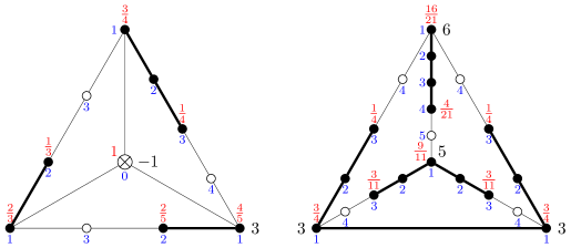
Figure 1. Surfaces with $(K_{X}+B)^{2}=\frac{1}{60}$ and $K_{X}^{2}=\frac{1}{462}$

Notation 4.1.

The large numbers are marks, when not equal to 1 or 2. The blue small numbers underneath are the weights, and the red fractional numbers on top are $b_{i}$, the negatives of discrepancies.

For the first pair $(X,B)$ one has $\epsilon_{1}=1-\frac{1}{3}-\frac{1}{4}-\frac{1}{5}=\frac{13}{60}$. There is an alternative choice of weights $(1,3,4,5)$ in this case, for which this pair fits into the case (3) of Lemma 3.3, i.e. all edges are CY. Then $\delta_{1}=\frac{1}{13}$ by Lemma 3.4, and $(K+B)^{2}=\frac{13}{60}\cdot\frac{1}{13}=\frac{1}{60}$. In fact, another description for this pair is $(X,B)=({\mathbb{P}}(3,4,5),D_{13})$ where $D_{13}$ is a degree 13 weighted hypersurface, and this is exactly Kollár’s example from [Kol13]. One has $\rho(X)=\operatorname{rank}\operatorname{Pic}X=1$, and $K_{X}+B$, $B$, and $-K_{X}$ are ample.

For the second pair we can also choose the weights $(1-2\epsilon,1,1+\epsilon,1+\epsilon)$, $0<\epsilon<\frac{1}{2}$, for which (2.1), (3.1) give that $K_{X}$ is ample and not just big and nef.

5. Example with nonempty boundary: $1/{462}$

Figure 2 shows two non-isomorphic visible graphs producing pairs $(X,B)$ of the smallest volume with nonempty boundary that we were able to find by our method.

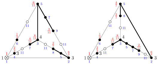
Figure 2. Surfaces with $(K_{X}+B)^{2}=\frac{1}{462}=\frac{1}{11\cdot 42}$ and $B\neq 0$

The winning weights are $(1,2,3,5)$. Both pairs achieve the minimal possible value of $\epsilon_{1}=1-\frac{1}{2}-\frac{1}{3}-\frac{1}{7}=\frac{1}{42}$. On the other hand, one has $K_{X}+B\equiv\frac{1}{11}B$ and $\delta_{1}=\frac{1}{11}$ by Lemma 3.4. Thus, one has $(K_{X}+B)^{2}=\epsilon_{1}\delta_{1}$. The divisor $K_{X}+B$ is big and nef but there are no weights for which (2.1), (3.1) or a variation of them show that $K_{X}+B$ is ample. The canonical model has ample $K_{X_{\rm can}}+B_{\rm can}$ and $(K_{X_{\rm can}}+B_{\rm can})^{2}=(K_{X}+B)^{2}=\frac{1}{462}$.

Notation 5.1.

We use Figure 2 for an alternative labeling of the curves, as follows. We denote the strict preimages of the four lines by ${\widetilde{L}}^{w}$, where the superscript $w=1,2,3,5$ is the (blue) weight of the corresponding vertex. Similarly, we denote one of the remaining curves by ${\widetilde{F}}_{w}^{i,j}$ if its vertex lies on the edge between ${\widetilde{L}}^{i},{\widetilde{L}}^{j}$ and has weight $w$. In the same vein, we call the initial lines in the plane $L^{w}$ and the intersection points $P^{i,j}=L^{i}\cap L^{j}$.

Finally, we use this labeling for the standard orthogonal basis of $\operatorname{Pic}{\widetilde{X}}$ consisting of the pullback $H$ of a line from ${\mathbb{P}}^{2}$ and the full preimages of the $(-1)$-curves from the intermediate blowups ${\widetilde{X}}\to{\mathbb{P}}^{2}$. Thus, in $\operatorname{Pic}{\widetilde{X}}$ we have ${\widetilde{L}}^{1}=H-F^{1,3}_{4}-F^{1,5}_{6}$, ${\widetilde{F}}^{1,3}_{4}=F^{1,3}_{4}-F^{1,3}_{7}-F^{1,3}_{11}$, ${\widetilde{F}}^{1,3}_{7}=F^{1,3}_{7}-F^{1,3}_{11}$, ${\widetilde{F}}^{1,3}_{11}=F^{1,3}_{11}$, etc.

Theorem 5.2.

The two visible graphs of Figure 2 describe the same surface $X$. If $\operatorname{char}k\neq 2$ then $K_{X}+B$ is ample, $\rho(X)=2$, and $X=X_{\rm can}$ has 4 singularities. If $\operatorname{char}k=2$ then $K_{X}+B$ is big, nef, but not ample, and it contracts a $(-2)$-curve. One has $\rho(X_{\rm can})=~{}1$, and $X_{\rm can}$ has 5 singularities, the last one a simple $A_{1}$.

Proof.

The second graph has an extra $(-1)$-curve $F^{1,5}_{11}$ not present in the first graph. It is easy to see that with respect to the first graph it is simply the strict preimage of the line in ${\mathbb{P}}^{2}$ connecting the points $P^{1,5}$ and $P^{2,3}$. Thus, the surfaces are the same but different curves are illuminated as being visible.

Let us work with the first representation. Suppose that there exists another, not visible curve ${\widetilde{D}}$ such that ${\widetilde{D}}\cdot\pi^{*}K_{X}=0$, which is then contracted by a linear system $|N\pi^{*}K_{X}|$ for $N\gg 0$. Since $\rho(X)=2$, there could only be one such irreducible curve. We write ${\widetilde{D}}=dH-\sum m^{ij}_{w}F^{ij}_{w}.$ The divisor ${\widetilde{D}}$ intersects by zero the curves ${\widetilde{L}}^{1}$, ${\widetilde{F}}^{1,3}_{4}$, ${\widetilde{F}}^{1,5}_{6}$, ${\widetilde{L}}^{2}$, ${\widetilde{F}}^{2,3}_{5}$, ${\widetilde{F}}^{2,3}_{8}$ since the full pullback $\pi^{*}K_{X}=\frac{1}{11}\pi^{*}B_{0}$ is a strictly positive combination of these curves. Also, ${\widetilde{D}}$ intersects non-negatively all the other visible curves. This gives an explicit set of identities and inequalities. One checks that the only solution is

$${\widetilde{D}}=c\big{[}3H-(2F^{1,3}_{4}+F^{1,3}_{7}+F^{1,3}_{11})-(F^{1,5}_{6}+F^{1,5}_{11})-(F^{2,5}_{7}+F^{2,5}_{9}+F^{2,5}_{11})\big{]}.$$

Then ${\widetilde{D}}K_{\widetilde{X}}=0$ and ${\widetilde{D}}^{2}=-2c^{2}$. It follows from the genus formula that $c=1$, and ${\widetilde{D}}$ is a smooth rational $(-2)$-curve. It must be a strict preimage of a cubic curve $D$ in ${\mathbb{P}}^{2}$ which has:

1. a cusp at $P^{1,3}$ with the tangent direction $L^{3}$,

2. a flex at $P^{2,5}$ with the tangent direction $L^{2}$,

3. a tangent at $P^{1,5}$ to the line $L^{5}$.

Thus, $D$ is a cuspidal cubic, and the set of points of $D\setminus P^{1,3}$ has the structure of the additive group ${\mathbb{G}}_{a}$. We see that the cubic $D$ with the above properties exists if and only if the system of equations $3P^{2,5}=P^{2,5}+2P^{1,5}=0$ has a solution in the base field $k$ with $P^{2,5}\neq P^{1,5}$. This is possible iff $\operatorname{char}k=2$; then $P^{2,5}=0$ and $P^{1,5}$ is any other smooth point. This completes the proof.

A second proof using the alternative presentation of surface $X$ works in characteristics 2 and 0, and by extension in all but finitely many other positive characteristics. The second visible graph of Figure 2 leads to a smooth rational $(-2)$-curve

$${\widetilde{D}}=4H-(2F^{1,3}_{4}+F^{1,3}_{7}+F^{1,3}_{11})-(2F^{1,5}_{6}+2F^{1,5}_{11})-(F^{2,3}_{5}+F^{2,3}_{7}+F^{2,3}_{9}+F^{2,3}_{11}).$$

It must be then a strict preimage of a quartic curve $D$ on ${\mathbb{P}}^{2}$ that has:

1. an $A_{2}$-singularity (a cusp) at $P^{1,3}$ with the tangent line $L^{3}$,

2. an $A_{3}$ (a tachnode) or $A_{4}$-singularity at $P^{1,5}$ with the tangent line $L^{5}$,

3. a hyperflex at $P^{2,3}$ with the tangent direction $L^{2}$, i.e. $L^{2}\cap D$ is a smooth point of $D$ and the intersection is of multiplicity $4$.

If $\operatorname{char}k=0$ then such quartic curves do not exist. Indeed, [Wal95a, Table 2] shows that irreducible quartic curves in characteristic 0 with $A_{2}A_{3}$ or $A_{2}A_{4}$ singularities do not have any hyperflexes. Since the property of $K_{X}+B$ being ample is open, the same is true in all but finitely many prime characteristics. On the other hand, if $\operatorname{char}k=2$ then there exists a unique such curve (with $A_{2}A_{3}$), which can be concluded from the normal forms of quartics given in [Wal95b]. Explicitly, the equation of $D$ can be taken to be $f=x^{4}+x^{2}yz+x^{2}y^{2}+y^{2}z^{2}$ and the lines are $L^{1}=(x)$, $L^{2}=(y+z)$, $L^{3}=(x+z)$, $L^{5}=(y)$. ∎

Remark 5.3.

Combining the two presentations of surface $X$ in the proof, we see that a quartic with the above configuration of singularities and tangent lines does not exist in prime characteristics $p\neq 2$.

Remark 5.4.

The intersections of ${\widetilde{D}}$ with the visible curves are zero except for the following:

1. For the first graph, ${\widetilde{D}}{\widetilde{F}}^{1,3}_{11}={\widetilde{D}}{\widetilde{F}}^{1,5}_{11}={\widetilde{D}}{\widetilde{F}}^{2,3}_{11}=1$.

2. For the second graph, ${\widetilde{D}}{\widetilde{F}}^{1,5}_{11}=2$ and ${\widetilde{D}}{\widetilde{F}}^{1,3}_{11}={\widetilde{D}}{\widetilde{F}}^{2,3}_{11}=1$.

6. Example with empty boundary: $1/{$48983$}$

There exist at least four visible graphs that produce surfaces $X$ without a boundary and $K_{X}^{2}=\frac{1}{$48983$}=\frac{1}{11\cdot 61\cdot 73}$. Three of them share the same list of singularities; the list is different for the fourth graph. The first two graphs can be obtained directly by inserting 10 vertices into the edge from ${\widetilde{L}}^{1}$ to ${\widetilde{L}}^{2}$, i.e. by blowing up the surfaces ${\widetilde{X}}$ of Figure 2 above the point $P^{1,2}$ 10 times. We show one of these surfaces in Figure 3. It leads to a surface with $\rho(X)=2$ and three singularities.

The fourth graph describes a surface $X^{\prime}$ with $\rho(X^{\prime})=3$ which has four singularities: the singularity with the minimal resolution $[2,4,2,2,2]$ of Figure 3 is replaced by two singularities $[2,6]$ and $[2,3,2,2]$.

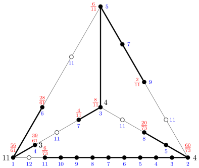
Figure 3. Surface with $K_{X}^{2}=\frac{1}{$48983$}=\frac{1}{11\cdot 61\cdot 73}$

The set of winning weights in these cases is again $(1,2,3,5)$. Since $$48983$>42^{2}$, these examples show that $K^{2}({\mathcal{S}}_{1})$ is achieved when the boundary is empty, that is, $K^{2}_{1}({\mathcal{S}}_{1})>K^{2}({\mathcal{S}}_{1})=K^{2}({\mathcal{S}}_{0})$.

Similarly to the previous case, the divisor $K_{X}$ is big and nef but there are no weights for which (2.1), (3.1) or a variation of them show that $K_{X}$ is ample. But the canonical model $X_{\rm can}$ has ample canonical class and $K_{X_{\rm can}}^{2}=K_{X}^{2}=\frac{1}{$48983$}$.

Theorem 6.1.

The three distinct visible graphs describe the same surface $X$. The fourth graph describes a different surface $X^{\prime}$ which however has the same canonical model since there is a crepant blow down $X^{\prime}\to X$ contracting the image of a $(-1)$-curve from ${\widetilde{X}}^{\prime}$. If $\operatorname{char}k\neq 2$ then $K_{X}$ is ample, $\rho(X)=2$, and $X=X_{\rm can}$ has 3 singularities. If $\operatorname{char}k=2$ then $K_{X}$ is big, nef, but not ample, and it contracts a $(-2)$-curve; $\rho(X_{\rm can})=~{}1$, and $X_{\rm can}$ has 4 singularities, the last one a simple $A_{1}$.

Proof.

The proof of the equivalence for the first three graphs is the same as in Theorem 5.2. Since the surface in the end is unique we do not draw the other two graphs but indicate the two invisible curves that have to be added to Figure 3 to obtain them. These are the strict preimages of a line in ${\mathbb{P}}^{2}$ joining $P^{1,5}$ and $P^{2,3}$, and of a conic passing through $P^{1,2}$ generically, through $P^{1,5}$ with the tangent $L^{5}$, and through $P^{2,3}$ with the tangent $L^{3}$.

Similarly, the surface $X^{\prime}$ described by a fourth graph, which we do not draw, has an invisible curve $C$, a strict preimage of a line through $P^{1,2}$ and $P^{3,5}$ such that $C\cdot\pi^{*}K_{X^{\prime}}=0$. Contracting this curve gives the same surface as in Figure 3.

From now on, we work with the surface $X$ described by Figure 3. Again, if there exists an invisible curve ${\widetilde{D}}$ with ${\widetilde{D}}\cdot\pi^{*}K_{X}=0$ then it must have zero intersection with the curves effectively supporting $\pi^{*}K_{X}$, which include the 10 newly inserted curves ${\widetilde{F}}^{12}_{w}$. Thus, the inequalities in this case are reduced to those in Theorem 5.2, and the rest of the proof is the same. ∎

As in Remark 5.4, the intersections of $D$ with the visible curves are zero except for those listed there.

7. Connection with the algebraic Montgomery-Yang problem

The algebraic Montgomery-Yang problem [Kol08, Conj. 30] asks whether there exists a surface with $\rho(S)=1$ and $\pi_{1}(S\setminus\operatorname{Sing}S)=1$ that has four quotient singularities. Conjecturally, the answer is no. All the possibilities for such surfaces were ruled out except when $K_{S}$ is ample, see [HK12].

It is amusing to note that if the characteristic 2 surface $S=X_{\rm can}$ with 4 singularities which we constructed in Theorem 6.1 existed in characteristic 0 then it would provide a counterexample to the above conjecture.

Let $U_{s}\ni s$ be a small neighborhood of a singular point $s$ and $L_{s}=U_{s}\setminus s$. Then the three singularities whose determinants $m=11,61,73$ are coprime to $2$ are quotient singularities and one has $\pi_{1}^{\rm alg}(L_{s})={\mathbb{Z}}_{m}$. For the fourth singularity obtained by contracting a $(-2)$-curve one has $\pi_{1}^{\rm alg}(L_{s})=1$ in characteristic 2. One can prove that $\pi_{1}^{\rm alg}(S\setminus\operatorname{Sing}S)=1$ by the usual methods, by considering the images of the $(-1)$-curves $C_{j}$ connecting the singularities and using van Kampen theorem, which still holds for the étale fundamental group in positive characteristic by [Gro63, IX, Th.5.1], cf. [MB12].

In any case, this surface also violates the orbifold Bogomolov-Miyaoka-Yau inequality $c_{1}^{2}(S)\leq 3e_{\rm orb}(S)$, for which one may see the discussion in [Kol08, §1]. Namely, it violates its corollary, the inequality

$$\sum_{s\in\operatorname{Sing}S}\left(1-\frac{1}{|\pi_{1}(U_{s}\setminus s)|}\right)\leq 3,$$

if one literally replaces $\pi_{1}$ with $\pi_{1}^{\rm alg}$, or if one replaces $|\pi_{1}(U_{s}\setminus s)|$ with $m_{i}$. Thus, this configuration of singularities can not appear in characteristic 0 if $\rho(X)=1$.

8. The case of Picard rank 1

In part because of the connection with the algebraic Montgomery-Yang problem, it is of interest to know the minimal volume for surfaces with the additional condition $\rho(X)=1$, in characteristic 0. For surfaces without the boundary, the best we were able to find is $K_{X}^{2}=\frac{1}{6351}=\frac{1}{3\cdot 29\cdot 73}$.

There are three possible graphs for the visible curves in this case, and one of them describes a surface that can be obtained by contracting two curves on the hypersurface in a weighted projective space from Example 1.3. Thus, it is one of the surfaces $S^{*}(2,2,4,10)$ studied in [Kol08, Sec.43].

The other two graphs are not of this type, and we give one of them in Figure 4. However, all three graphs share the same list of singularities. Indeed, the argument we gave in the proof of Theorems 5.2, 6.1 shows that the three visible graphs describe the same surface.

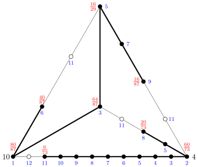
Figure 4. Surface with $K_{X}^{2}=\frac{1}{6351}=\frac{1}{3\cdot 29\cdot 73}$ and $\rho(X)=1$

Remark 8.1.

Comparing Figures 3 and 4, one can see that our surface with the minimal volume can be obtained from the surface $S^{*}(2,2,4,10)$ by a weighted blowup at one point.

In [HK12] Hwang and Keum construct, for any $a_{1},a_{2},a_{3},a_{4}\geq 2$, a surface $T=T(a_{1},a_{2},a_{3},a_{4})$ with $\rho(T)=1$ obtained by blowing up the 4-line configuration; it has two cyclic singularities corresponding to the chains $[2*(a_{4}-1),a_{3},a_{1},2*(a_{2}-1)]$ and $[2*(a_{3}-1),a_{2},a_{4},2*(a_{1}-1)]$. In particular, these surfaces include all the surfaces $S^{*}(a_{1},a_{2},a_{3},a_{4})$ with $\gcd(w_{1},w_{3})=\gcd(w_{2},w_{4})=1$ by [UYn16].

Theorem 8.2.

Let

$$A = a_{1}a_{2}a_{3}a_{4}-a_{2}a_{3}a_{4}-a_{1}a_{3}a_{4}-a_{1}a_{2}a_{4}-a_{1}a_{2}a_{3}+$$

$$a_{1}a_{2}+a_{2}a_{3}+a_{3}a_{4}+a_{1}a_{4}-a_{1}-a_{2}-a_{3}-a_{4}+3$$

$$B_{1} = a_{1}a_{2}a_{3}a_{4}-a_{1}a_{3}a_{4}-a_{1}a_{2}a_{3}+a_{2}a_{3}+a_{1}a_{4}-a_{1}-a_{3}+1$$

$$B_{2} = a_{1}a_{2}a_{3}a_{4}-a_{2}a_{3}a_{4}-a_{1}a_{2}a_{4}+a_{1}a_{2}+a_{3}a_{4}-a_{2}-a_{4}+1$$

Then the following is true:

1. The surface $T(a_{1},a_{2},a_{3},a_{4})$ has ample canonical class $K_{T}$ iff $A>0$.

2. The determinants of the two singularities are $B_{1}$ and $B_{2}$.

3. $K_{T}^{2}=A^{2}/B_{1}B_{2}.$

4. The minimum $K_{T}^{2}=\frac{1}{6351}$ is achieved for $(a_{i})=(2,2,4,10)$, up to a cyclic rotation.

Proof.

(1) We compute $\pi^{*}K_{X}\cdot C$ for a $(-1)$-curve $C$ by Lemma 2.5(1) and find that it is a product of $A$ and some positive terms.

(2) is [HK12, Lemma 2.4].

(3) follows by a direct computation, applying Lemma 2.5(2).

(4) It is somewhat more convenient to use the variables $x_{i}=a_{i}-1$. Then

$$\frac{A}{x_{1}x_{2}x_{3}x_{4}}=1-\frac{1}{x_{1}}\frac{1}{x_{3}}\left(1+\frac{1}{x_{2}}+\frac{1}{x_{4}}\right)-\frac{1}{x_{2}}\frac{1}{x_{4}}\left(1+\frac{1}{x_{1}}+\frac{1}{x_{3}}\right).$$

One easily checks that for $j=1,2$ the partial derivatives $\partial(A/B_{j})/\partial x_{i}\geq 0$ when $A>0$ and $x_{i}\geq 1$. Thus, it is sufficient to check the minimal collections $(a_{i})$ for which $A>0$, meaning: for any other collection $(a_{i}^{\prime})$ with $A>0$ one has $a_{i}^{\prime}\geq a_{i}$ $\forall i$.

We first find the “critical” collections, for which $A=0$. These are $(3,3,3,3)$, $(2,8,3,3)$, $(2,3,\frac{11}{2},3)$, $(2,3,3,8)$, $(2,2,4,9)$, $(2,2,5,6)$, $(2,2,6,5)$, $(2,2,9,4)$.

Then, modulo rotational symmetry, the smallest collections $(a_{i})$ for which $A>0$ are $(4,3,3,3)$, $(2,9,3,3)$, $(2,8,4,3)$, $(2,8,3,4)$, $(2,3,6,3)$, $(2,4,3,8)$, $(2,3,4,8)$, $(2,3,3,9)$, $(3,2,4,9)$, $(2,3,4,9)$, $(2,2,5,9)$, $(2,2,4,10)$, $(3,2,5,6)$, $(2,3,5,6)$, $(2,2,6,6)$, $(2,2,5,7)$, $(3,2,6,5)$, $(2,3,6,5)$, $(2,2,7,5)$, $(2,2,6,6)$, $(2,3,9,4)$, $(2,2,10,4)$, $(2,2,9,5)$. Among these, the minimal value $A^{2}/B_{1}B_{2}=\frac{1}{6351}$ is achieved for $(a_{1},a_{2},a_{3},a_{4})=(2,2,4,10)$. ∎

For the surfaces with boundary, we found a pair with $(K_{X}+B_{0})^{2}=\frac{1}{78}$. The marks of the corners are 1, 3, $2^{\prime}$, $2^{\prime\prime}$ ($B_{0}$ goes first, we use the notation $2^{\prime},2^{\prime\prime}$ to distinguish the two vertices with the same marks), and the curves along the edges have marks 1–3, 1–2–2–1–$2^{\prime}$, 1–2–1–$2^{\prime\prime}$, 3–$2^{\prime}$, 3–1–2–2–2–$2^{\prime\prime}$, $2^{\prime}$–$2^{\prime\prime}$. The weights that work for Lemma 3.3(3) are $(1,1,2,3)$, $n=7$, $\delta_{1}=\frac{1}{7}$, and $\epsilon_{1}=1-\frac{1}{2}-\frac{1}{3}-\frac{1}{13}=\frac{7}{78}$.

9. Why only four lines?

It may seem naive and insufficient in search of examples to reduce oneself only to the simplest of line arrangements: four lines in the plane. Why not consider some more interesting configurations, e.g. a Fano or anti-Fano configuration of 7 lines or Segre (resp. dual Segre) configuration of 12 (resp. 9) lines? And why lines and not conics or curves of higher degree? In fact, there are good ad hoc reasons for this:

(1) For all examples of log surfaces arising from 4 lines, one apriori has $K_{X}^{2}\leq(K_{{\mathbb{P}}^{2}}+\sum_{i=0}^{3}L_{i})^{2}=1$. Similarly, for $d$ lines in general position an upper bound is $(d-3)^{2}$. For special line arrangements the upper bound is smaller but it starts with 2 for a special configuration of 5 lines. Although this is an upper and not a lower bound, it shows how hard one has to work to achieve a minimum. Indeed, for $d\geq 7$ lines in general position it is easy to show that

$$K_{X}^{2}\geq 9-\frac{d(d-1)}{2}+\frac{d-4}{d-2}(d-4)d=\frac{d^{2}}{2}-\frac{11d}{2}+13+\frac{8}{d-2}\geq\frac{3}{5},$$

with the minimum achieved by blowing up all of the $\frac{d(d-1)}{2}$ intersection points of the $d$ lines.

(2) The combinatorial game, similar to the one we described in Section 3, becomes very hard to play for more than 4 lines. E.g., for 5 lines the condition on the weights becomes $w_{0}+\dotsb+w_{4}=2n$, and there are very few interesting examples. A similar thing happens if one works with conics instead of lines.

(3) We also note that constructions of many interesting log surfaces with ample $K_{X}$ can be reduced to blowups of the same 4-line configuration in ${\mathbb{P}}^{2}$, even when the initial definition is different, see e.g. [Kol08, HK11, HK12, UYn16]. The surfaces of [HK12] that use conics and cubics all have bigger volumes.

10. Lower bound for $K^{2}({\mathcal{S}}_{1})=K^{2}({\mathcal{S}}_{0})$.

In this section, we spell out the explicit effective lower bound for $K^{2}({\mathcal{S}}_{0})$ provided by Theorem 4.8 of [AM04]. In our present notations, it says the following:

$$K_{X}^{2}\geq\frac{1}{\ell\cdot(2\ell)^{N}},\quad\text{where }N=128\ell^{5}+4\ell\text{ and }\ell=\ulcorner 1/{\delta_{1}({\mathcal{S}}_{1})}\urcorner.$$

Together with Kollár’s bound $\delta_{1}({\mathcal{S}}_{1})\geq\frac{1}{42}$, this gives

$$K_{X}^{2}\geq\frac{1}{42\cdot 84^{128\cdot 42^{5}+4\cdot 42}}\approx 10^{-3.22\cdot 10^{10}}.$$

Certainly this is not a realistic bound. Many improvements can be made to the estimates in [AM04] but they would not cardinally change the estimate without introducing some cardinally new methods. The true lower bound for $K^{2}({\mathcal{S}}_{0})$ may be closer to Kollár’s conjectural bound for $K^{2}({\mathcal{S}}_{2})=\frac{1}{(42\cdot 43)^{2}}$. Indeed, we dare to think that it could be close, or equal to $\frac{1}{$48983$}\approx\frac{67}{(42\cdot 43)^{2}}$ that we give here.

References

- [Ale92] Valery Alexeev, Log canonical surface singularities: arithmetical approach, Flips and abundance for algebraic threefolds, Société Mathématique de France, Paris, 1992, Papers from the Second Summer Seminar on Algebraic Geometry held at the University of Utah, Salt Lake City, Utah, August 1991, Astérisque No. 211 (1992), pp. 47–58.
- [Ale94] by same author, Boundedness and for log surfaces, Internat. J. Math. 5 (1994), no. 6, 779–810.
- [AM04] Valery Alexeev and Shigefumi Mori, Bounding singular surfaces of general type, Algebra, arithmetic and geometry with applications (West Lafayette, IN, 2000), Springer, Berlin, 2004, pp. 143–174.
- [Art62] Michael Artin, Some numerical criteria for contractability of curves on algebraic surfaces, Amer. J. Math. 84 (1962), 485–496.
- [Bla95] Raimund Blache, An example concerning Alexeev’s boundedness results on log surfaces, Math. Proc. Cambridge Philos. Soc. 118 (1995), no. 1, 65–69.
- [Gro63] Alexander Grothendieck, SGA1-II. Revêtements étales et groupe fondamental. Fasc. II: Exposés 6, 8 à 11, Séminaire de Géométrie Algébrique, vol. 1960/61, Institut des Hautes Études Scientifiques, Paris, 1963.
- [HK11] Dongseon Hwang and Jonghae Keum, The maximum number of singular points on rational homology projective planes, J. Algebraic Geom. 20 (2011), no. 3, 495–523.
- [HK12] DongSeon Hwang and JongHae Keum, Construction of singular rational surfaces of Picard number one with ample canonical divisor, Proc. Amer. Math. Soc. 140 (2012), no. 6, 1865–1879.
- [Kol94] János Kollár, Log surfaces of general type; some conjectures, Classification of algebraic varieties (L’Aquila, 1992), Contemp. Math., vol. 162, Amer. Math. Soc., Providence, RI, 1994, pp. 261–275.
- [Kol08] by same author, Is there a topological Bogomolov-Miyaoka-Yau inequality?, Pure Appl. Math. Q. 4 (2008), no. 2, Special Issue: In honor of Fedor Bogomolov. Part 1, 203–236.
- [Kol13] by same author, Moduli of varieties of general type, Handbook of moduli. Vol. II, Adv. Lect. Math. (ALM), vol. 25, Int. Press, Somerville, MA, 2013, pp. 131–157.
- [Kou76] A. G. Kouchnirenko, Polyèdres de Newton et nombres de Milnor, Invent. Math. 32 (1976), no. 1, 1–31.
- [MB12] Laurent Moret-Bailly, An étale version of the van Kampen theorem, 2012, http://mathoverflow.net/questions/110511.
- [Miy01] Masayoshi Miyanishi, Open algebraic surfaces, CRM Monograph Series, vol. 12, American Mathematical Society, Providence, RI, 2001.
- [OR77] P. Orlik and R. Randell, The structure of weighted homogeneous polynomials, Several complex variables (Proc. Sympos. Pure Math., Vol. XXX, Part 1, Williams Coll., Williamstown, Mass., 1975), Amer. Math. Soc., Providence, R. I., 1977, pp. 57–64.
- [UYn16] Giancarlo Urzúa and José Ignacio Yáñez, Characterization of Kollár surfaces, Preprint (2016), arXiv:1612.01960.
- [Wal95a] C. T. C. Wall, Geometry of quartic curves, Math. Proc. Cambridge Philos. Soc. 117 (1995), no. 3, 415–423.
- [Wal95b] by same author, Quartic curves in characteristic , Math. Proc. Cambridge Philos. Soc. 117 (1995), no. 3, 393–414.