Bifurcation trees of Stark-Wannier ladders for accelerated BECs in an optical lattice

Abstract

In this paper we show that in the semiclassical regime of periodic potential large enough, the Stark-Wannier ladders become a dense energy spectrum because of a cascade of bifurcations while increasing the ratio between the effective nonlinearity strength and the tilt of the external field; this fact is associated to a transition from regular to quantum chaotic dynamics.  The sequence of bifurcation points is explicitly given.

The dynamics of a quantum particle in a periodic potential under an homogeneous external field is one of the most important problems in solid-state physics.  When the periodic potential is strong enough then we are in the semiclassical regime where tunneling between adjacent wells of the periodic potential is practically forbidden; in the opposite situation tunneling may occur and the particle performs Bloch oscillations.  Dynamics of particles become more interesting when we take into account the interaction among them, as we must do in the case of interacting ultracold atoms.  In fact, accelerated ultracold atoms moving in an optical lattice Bloch1 ; Bloch2 ; RSN ; SPSSKP ; Shin has opened the field to multiple applications, as well as the measurements of the value of the gravity acceleration $g$ using ultracold Strontium atoms confined in a vertical optical lattice FPST ; PWTAPT , direct measurement of the universal Newton gravitation constant $G$ RSCPT and of the gravity-field curvature RCSMPT .

Because of the periodicity of the potential associated to the optical lattice, it is expected the existence of families of stationary states with associated energies displaced on regular ladders, the so-called Stark-Wannier ladders WS ; GKK (see also REWWK for numerical computation of Stark-Wannier states for BECs in an accelerated optical lattice); this picture implies, at least for a single particle model, Bloch oscillations.  When one takes into account the binary particle interaction of the condensate nonlinear effects occur and new sub-harmonic oscillations appear S4 ; KKG ; WWMK .  More recently, Meinert et al MMKLWGN have observed that when the strength of the uniform acceleration is reduced a transition from regular to quantum chaotic dynamics is observed; in their experiments evidence of the fact that the energy spectrum emerges densely packed, as predicted by BK by means of a numerical simulation for a lattice with a finite number of wells, is given.

In fact, such a problem has been intensively studied in the recent years by means of numerical methods.  In LZG the authors consider a one-dimensional BEC of particles described by the Gross-Pitaevskii equation; they reduce the problem to a quasi-integrable dynamical system which displays classical-like Kolmogorov-Arnold-Moser structured chaos.  In HVZOMB the authors model the cloud of ultracold bosons in a tilted lattice by means of the Bose-Hubbard Hamiltonian that incorporates both the tunneling between neighboring sites and the on-site interaction; by means of such an approach they are able to identify regular structures in a globally chaotic spectra and the associated eigenstates exhibit strong localization properties in the lattice.  In KGK the authors, making use of the mean-field and single band approximations, describe the dynamics of a BEC in a tilted optical lattice by means of a discrete nonlinear Schrödinger equation; in the strong field limit they demonstrate the existence of (almost) non spreading states which remain localized on the lattice region populated initially.  Finally, VG can give numerical evidence of the quasi-classical chaos on the emergence of nonlinear dynamics.

In this paper we consider the dynamics of ultracold interacting atoms in a periodic potential subjected to an external force.  We can show a transition from the semiclassical picture, where each atom is localized on a single well of the periodic potential, to a chaotic picture, for strength of the nonlinearity term large enough, associated to a cascade of bifurcations of the energy spectrum; in particular, we can see that when the ratio between the effective strength of the nonlinearity interaction term and the strength of the external homogeneous field becomes larger of some given values then bifurcations of the stationary solutions occur and new stationary solutions localized on a larger number of wells appear.  In our model the structure of a bifurcation trees arising from the Wannier-Stark ladders clearly emerges and the sequence of bifurcation points is explicitly given.

Transversely confined BECs in a periodic optical lattice under the effect of the gravitational force are governed by the one-dimensional time-dependent Gross-Pitaevskii (GP) equation with a periodic potential and a Stark potential

$$i\hbar\partial_{t}\psi=-\frac{\hbar^{2}}{2m}\partial_{xx}^{2}+V(x)\psi+mgx\psi+\gamma|\psi|^{2}\psi$$ (1)

where the BEC’s wavefunction $\psi(x,t)$ has constant norm: $\|\psi(\cdot,t)\|_{L^{2}}=\|\psi_{0}(\cdot)\|_{L^{2}}$, where $\psi_{0}(x)$ is the initial wavefunction of the BEC, $m$ is the mass of the atoms, $g$ is the gravity acceleration, $\gamma$ is the one-dimensional nonlinearity strength and $V(x)$ is the periodic potential associated to the optical lattice potential.  In typical experiments Bloch1 the periodic potential has the usual shape $V(x)=V_{0}\sin^{2}(k_{L}x)$ where $b={\pi}/{k_{L}}$ is the period and $V_{0}=\Lambda_{0}E_{R}$ where $E_{R}$ is the photon recoil energy.

If one looks for stationary solutions

$$\psi(x,t)=e^{i\lambda t/\hbar}\psi(x)$$

to the time-dependent GP equation (1) it turns out that $\lambda$ is real-valued and that $\psi(x)$ is a solution to the time-independent GP equation; then, we may assume that $\psi(x)$ is a real-valued function by means of a gauge argument (see Lemma 3.7 by P ).  Hence, the time-independent GP equation becomes

$$\lambda\psi=-\frac{\hbar^{2}}{2m}\partial_{xx}^{2}\psi+V(x)\psi+mgx\psi+\gamma\psi^{3}$$ (2)

where $\psi(x)$ is a real valued function.  First of all let us remark that the stationary solutions to eq. (2), if there, must be displaced on regular ladders.  Indeed eq. (2) is invariant by translation $x\to x+b$ and $\lambda\to\lambda-mgb$, because $V(x+b)=V(x)$ where $b$ is the lattice’s period.  Thus we have families of stationary solutions $(\lambda_{j},\psi_{j}(x))$, $j\in{\mathbb{Z}}$, where $\lambda_{j}=\lambda_{0}+jmgb$ and $\psi_{j}(x)=\psi_{0}(x-jb)$ for some $\lambda_{0}$ and $\psi_{0}(x)$.  Therefore, we can restrict our analysis to just one rung of the ladder and then we replicate the obtained results to all other rungs.

By means of the tight-binding approach we reduce equation (2) to a discrete nonlinear Schrödinger equation.  The idea is basically simple FS and it consists in assuming that the wavefunction $\psi(x)$, when restricted to the first band of the periodic Schrödinger operator, may be written as a superposition of vectors $u_{\ell}(x)$ localized on the $\ell$-th well of the periodic potential; i.e. $\psi(x)=\sum_{\ell\in{\mathbb{Z}}}c_{\ell}u_{\ell}(x)$, for some $c_{\ell}$.  If $u_{\ell}(x)$ are real-valued functions then the parameters $c_{\ell}$ are real valued too.  For instance $u_{\ell}(x)=W_{1}(x-x_{\ell})$ where $W_{1}(x)$ is the Wannier function associated to the first band and $x_{\ell}=\ell b$ is the center of the $\ell$-th well.  Let $\mathbf{c}=\{c_{\ell}\}_{\ell\in{\mathbb{Z}}}\in\ell^{2}({\mathbb{Z}})$ be the representation of the wave-vector $\psi(x)$ in the tight binding approximation.  Therefore, the tight-binding approach lead us to a system of discrete nonlinear Schrödinger equations which dominant terms are given by

$$\lambda c_{\ell} = (\lambda_{D}+mgC_{0})c_{\ell}-\beta(c_{\ell+1}+c_{\ell-1})+$$ (3)

$$\ \ +\gamma\|u_{0}\|_{L^{4}}^{4}c_{\ell}^{3}+mgb\ell c_{\ell}\,,\ \ell\in{\mathbb{Z}}\,,$$

where $\lambda_{D}$ is the ground state of a single well potential and where $\beta$ is the hopping matrix element between neighboring wells, and $C_{0}=\int_{{\mathbb{R}}}x|u_{0}(x)|^{2}dx$.  By means of a simple recasting $\mu=\lambda-\mu^{\star}$, $\mu^{\star}=(\lambda_{D}+mgC_{0}+2\beta)$, $\nu=\gamma\|u_{0}\|_{L^{4}}^{4}$ and $f=mgb$, then equation (3) takes the form

$$\mu c_{\ell}=-\beta(c_{\ell+1}+c_{\ell-1}+2c_{\ell})+\nu c_{\ell}^{3}+f\ell c_{\ell}\,,\ \ell\in{\mathbb{Z}}\,,$$ (4)

where $c_{\ell}$ are real-valued and such that $\sum_{\ell\in{\mathbb{Z}}}c_{\ell}^{2}=1$; the parameter $\nu$ will play the role of the effective strength of the nonlinearity interacting term.  The theoretical question about the validity of the nearest-neighbor model (4) has been largely debated.  In particular, numerical experiments AKKS ; EHLZCMA suggest that the nearest-neighbor model properly works when $\Lambda_{0}$ is large enough, typically $\Lambda_{0}\geq 10$.

Localized modes of the discrete nonlinear Schrödinger equation (4) have been already studied by FS ; PS ; PSM when the external homogeneous external field is absent (i.e. when $f=0$).  In particular we should mention the contribution given by ABK where all the solutions obtained in the anticontinuous limit can be classified and where bifurcations are observed.  As far as we know the same analysis is still missing for equation (4) when $f\not=0$.  We look for solutions to the stationary equation (4) when $\Lambda_{0}$ is large enough; in such a case, by means of semiclassical arguments, it turns out that $\beta$ becomes small and the stationary solutions are close to the ones obtained in the anticontinuum limit of $\beta\to 0$, where (4) reduces to

$$\mu c_{\ell}=\nu c_{\ell}^{3}+f\ell c_{\ell}\,,\ \ell\in{\mathbb{Z}}\,.$$ (5)

When the nonlinear term is absent, that is $\nu=0$, then we simply obtain a family of solutions $\mu_{j}=fj$, for any $j\in{\mathbb{Z}}$, with associated stationary solutions $\mathbf{c}=\pm\{\delta_{j}^{\ell}\}_{\ell\in{\mathbb{Z}}}$.  In this case we recover the Wannier-Stark ladders WS ; GKK .

Assume now that the nonlinear term is not zero, that is $\nu>0$ for argument’s sake.  In general (5) has finite mode solutions ${\mathbf{c}}^{S}=\{c_{\ell}^{S}\}_{\ell\in{\mathbb{Z}}}$, associated to sets $S\subset{\mathbb{Z}}$ (hereafter called solution-sets) with finite cardinality ${\mathcal{N}}=\sharp S<\infty$, given by

$$c^{S}_{\ell}=\left\{\begin{array}[]{ll}0&\ \mbox{ if }\ell\notin S\\ \pm\left[\frac{\mu^{S}-f\ell}{\nu}\right]^{1/2}&\ \mbox{ if }\ell\in S\end{array}\right.\,,$$ (8)

with the condition

$$\frac{\mu^{S}}{f}>\max S\,,$$ (9)

because we have assumed that $c_{\ell}^{S}$ are real-valued and $\nu>0$.  Furthermore, since the stationary problem (5) is translation invariant $\ell\to\ell+1$ and $\mu\to\mu-f$ then we can always restrict ourselves to the rung of the ladder such that $\min S=0$, that is the solution-set has the form $S=\{0,\ell_{1},\,\ldots\,,\ell_{{\mathcal{N}}-1}\}$ with $0<\ell_{1}<\ell_{2}<\ldots<\ell_{{\mathcal{N}}-1}$ positive and integer numbers.  The normalization condition reads

$$1=\sum_{\ell\in S}(c_{\ell}^{S})^{2}=\sum_{\ell\in S}\left[\frac{\mu^{S}-f\ell}{\nu}\right]\,,$$ (10)

from which it follows that the energy $\mu$ is given by

$$\mu^{S}=\frac{\nu}{\mathcal{N}}+\frac{f}{\mathcal{N}}\sum_{\ell\in S}\ell\,.$$

Hence, condition (9) implies the following condition on the solution-set $S$

$$\frac{\nu}{f}>{\mathcal{N}}\max S-\sum_{\ell\in S}\ell=\sum_{\ell\in S}\left[\max S-\ell\right]\,.$$ (11)

In order to characterize the solution-sets $S$ let us introduce the complementary set $S^{\star}$ of $S$ defined as follows

$$S^{\star}=\{\ell^{\star}:=\max S-\ell\ :\ \ell\in S\}\,;$$

hence condition (11) becomes

$$\frac{\nu}{f}>\sum_{\ell^{\star}\in S^{\star}}\ell^{\star}\,.$$ (12)

Let us now denote by ${\mathcal{S}}^{\star}(\nu/f)$ the collection of sets $S^{\star}$ satisfying (12); let us also denote by ${\mathcal{Q}}^{\star}(n)$ the collection of sets of all non negative integer numbers, including the number $0$, which sum is equal to $n$, without regard to order with the constraint that all integers in a given partition are distinct; e.g. ${\mathcal{Q}}^{\star}(1)=\left\{\{0,1\}\right\}$, ${\mathcal{Q}}^{\star}(2)=\left\{\{0,2\}\right\}$ and ${\mathcal{Q}}^{\star}(3)=\left\{\{0,3\},\,\{0,1,2\}\right\}$.  Hence, by construction

$${\mathcal{S}}^{\star}(n+1)={\mathcal{S}}^{\star}(n)\cup{\mathcal{Q}}^{\star}(n)\,.$$

In conclusion, we have shown that the counting function ${F}(\nu/f)$ given by the number of solution-sets $S$ of integer numbers satisfying the conditions (11) and such that $\min S=0$, is given by

$${F}(\nu/f)=\sum_{0<n<\nu/f}Q(n)\,;$$ (13)

where $Q(n)$ (see Abramowitz and Stegun AS , p. 825) gives the number of ways of writing the integer $n$ as a sum of positive integers without regard to order with the constraint that all integers in a given partition are distinct; e.g. ${F}(3.1)=Q(1)+Q(2)+Q(3)=1+1+2=4$.

It turns out that ${F}(\nu/f)$ grows quite fast, indeed the following asymptotic behavior holds true AS :

$$Q(n)\sim\frac{e^{\pi\sqrt{n/3}}}{4\cdot 3^{1/4}n^{3/4}}\ \mbox{ as }\ n\to\infty\,.$$

Hence

$${F}(n)\sim\frac{\exp\left[{\pi}(n/3)^{1/2}\right]}{2{\pi}(n/3)^{1/4}}$$

as $n$ goes to infinity.

A cascade of bifurcation points, when $\nu/f$ takes the value of any positive integer, occurs; indeed, when the ratio $\nu/f$ becomes larger than a positive integer $n$ then $Q(n)$ new stationary solutions appear.  This fact can be seen in Figure 1, where we plot the values of the energy ${\mu}$, when $\nu/f$ belongs to the interval $[0,10]$, associated to the solution-sets $S$ such that $\min S=0$.  By translation $\mu\to\mu+jf$, $j\in{\mathbb{Z}}$, we must replicate this picture to the general situation where $\min S=j$, $j\in{\mathbb{Z}}$; that is this picture occurs for each rung of the ladder and then the collection of values of $\mu$ associated to stationary solutions is going to densely cover the whole real axis.

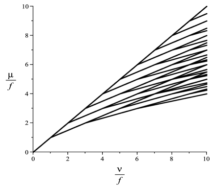
Figure 1: Here we plot the values of the energy $\mu/f$ associated to stationary solution-sets $S$ such that $\min S=0$; we can see a cascade of bifurcations when $\nu/f$ increases.  This picture occurs for each rung of the ladder.

If one looks with more detail the bifurcation cascade one can see that we have ${\mathcal{N}}$-mode solutions for any value of ${\mathcal{N}}$.  For instance, for ${\mathcal{N}}=1$ we have 1-mode solutions associated to solution-sets $S=\{j\}$, for any $j\in{\mathbb{Z}}$, given by $\mu^{\{j\}}=\nu+fj$ and ${\mathbf{c}}^{\{j\}}=\pm\{\delta_{\ell}^{j}\}_{\ell\in{\mathbb{Z}}}$.  That is we recover the (perturbed) Wannier-Stark ladder.

For ${\mathcal{N}}=2$ we have two-mode stationary solutions associated to solution-sets of the form $S=\{j,j+\ell_{1}\}$ for any $j\in{\mathbb{Z}}$ and $\ell_{1}\in{\mathbb{N}}$, where

$$\mu^{\{j,j+\ell_{1}\}}=\frac{1}{2}\nu+jf+\frac{1}{2}f\ell_{1}$$

under the condition $\ell_{1}>{\nu}/{f}$.  Therefore, we can conclude that $2$-mode solutions exists only if ${\nu}/{f}>1$, and the elements of the vector ${\mathbf{c}}^{\{j,j+\ell_{1}\}}$ are given by

$$c^{\{j,j+\ell_{1}\}}_{\ell}=\left\{\begin{array}[]{ll}0&\mbox{ if }\ell\not=j,j+\ell_{1}\\ \pm\left[\frac{1}{2}+\frac{1}{2}\frac{f}{\nu}\ell_{1}\right]^{1/2}&\mbox{ if }\ell=j\\ \pm\left[\frac{1}{2}-\frac{1}{2}\frac{f}{\nu}\ell_{1}\right]^{1/2}&\mbox{ if }\ell=j+\ell_{1}\end{array}\right.$$

In general, ${\mathcal{N}}$-mode stationary solutions are associated to solution-sets of the form

$$S=\{j,\ j+\ell_{1},\ \ldots\ ,\ j+\ell_{{\mathcal{N}}-1}\}$$ (15)

where $j\in{\mathbb{Z}}$ and $0<\ell_{1}<\ell_{2}<\ldots<\ell_{{\mathcal{N}}-1}\in{\mathbb{N}}$, the value of $\mu^{S}$ is given by

$$\mu^{S}=\frac{\nu}{{\mathcal{N}}}+jf+\frac{f}{{\mathcal{N}}}\sum_{r=1}^{{\mathcal{N}}-1}\ell_{r}$$

under condition (9).  As a particular family of ${\mathcal{N}}$-mode solutions we consider solution-sets of the form (15) for any $j\in{\mathbb{Z}}$ and $\ell_{r+1}-\ell_{r}=1$.  They are associated to

$$\mu^{S}=\frac{\nu}{{\mathcal{N}}}+fj+\frac{1}{2}f({\mathcal{N}}-1)$$

and then condition (9) implies that

$$\frac{{\mathcal{N}}({\mathcal{N}}-1)}{2}<\frac{\nu}{f}$$

Hence, we can observe a second bifurcation phenomenon: stationary solutions associated to solution-sets with ${\mathcal{N}}$ elements arises from solution-sets with ${\mathcal{N}}-1$ elements when $\nu/f$ becomes bigger than the critical value $(\nu/f)^{\mathcal{N}}={{\mathcal{N}}({\mathcal{N}}-1)}/{2}$.

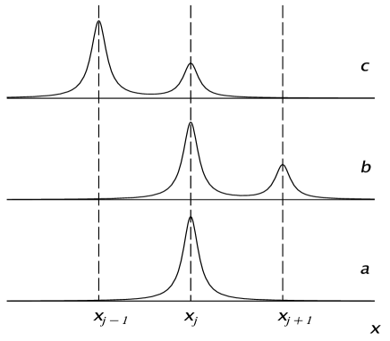
Figure 2: Here we plot the absolute value of the stationary solutions associated to the solution-sets $S_{1}$ (fig. a), $S_{2}$ (fig. b) and $S_{3}$ (fig. c); $x_{j}$ denotes the center of the $j$-th well of the periodic potential.

In order to understand the effect of such a stationary solutions on the BEC’s dynamics we consider, at first, the case where $\nu/f$ is less than one; then we have a family of solutions of the form $\psi(x,t)=e^{i(\mu+\mu^{\star})t/\hbar}u_{j}(x)$ where $\mu=\nu+jf$ and where $u_{j}(x)$ is localized on the $j$-th well of the periodic potential, $j\in{\mathbb{Z}}$.  In fact, in such a case the there is no interaction among these solutions, and the density of probability to find the state in the $j$-th well is time independent.  Let us consider now the case when $\nu/f$ is bigger that $1$, i.e. $\nu/f=3/2$ for argument’s sake; then in such a case we have that different stationary solutions may be supported on the same well of the periodic potential.  In particular, let us fix our attention on a given well with index $j$, then we have $3$ stationary solutions localized on the $j$-th well associated to the solution-sets (see Figure 2)

$$\begin{array}[]{ll}S_{1}=\{j\};&\mu^{S_{1}}=\nu+fj\\ S_{2}=\{j,j+1\};&\mu^{S_{2}}=\frac{1}{2}\nu+fj+\frac{1}{2}f\\ S_{3}=\{j-1,j\};&\mu^{S_{3}}=\frac{1}{2}\nu+fj-\frac{1}{2}f\end{array}$$

If we consider the superposition of these stationary solutions on the $j-$th well then it behaves like

$$e^{i\mu^{\star}t/\hbar+i\nu t/2\hbar+ifjt/\hbar}q(t^{\prime})u_{j}(x)$$

where we set $t^{\prime}=ft/\hbar$ and

$$q(t^{\prime})=\left[c_{j}^{S_{1}}e^{i\nu t^{\prime}/2f}+e^{it^{\prime}/2}c_{j}^{S_{2}}+e^{-it^{\prime}/2}c_{j}^{S_{3}}\right]$$ (17)

where $c^{S_{1}}_{j}=\pm 1$, $c_{j}^{S_{2}}=\pm\left[\frac{5}{6}\right]^{1/2}$, $c_{j+1}^{S_{2}}=\pm\left[\frac{5}{6}\right]^{1/2}$, $c_{j-1}^{S_{3}}=\pm\left[\frac{5}{6}\right]^{1/2}$, $c_{j}^{S_{3}}=\pm\left[\frac{1}{6}\right]^{1/2}$.  As a result we observe a beating behavior of the density of probability associated to different frequencies; one beating motion has period $2\pi$, which is $\nu$-independent and it coincides with the period of the Bloch oscillations, a second beating motion has two periods depending on $\nu/f$ given by $T_{1}=4\pi\left[1+\nu/f\right]^{-1}$ and $T_{2}=4\pi\left[-1+\nu/f\right]^{-1}$.  For bigger values of $\nu/f$ then we may consider a larger number of stationary solutions which all supports contain a fixed and given well, then the behavior on this given well of the superposition of such a stationary solutions will be given by means of a periodic function with period $2\pi$, coinciding with the Bloch period, plus a large number of periodic functions with different periods; since the number of these periodic functions will increase when the ratio $\nu/f$ increases then we expect a chaotic behavior for large $\nu/f$.  In fact, we should underline that a linear combination (like (17)) of stationary solutions to a nonlinear equation is not, in general, a solution to the same equation.  However, if we consider the limit of small $\nu$ (provided that $\nu/f$ is much bigger than $1$) then we can expect that, for fixed times, the contribution due to the non linear perturbation may be estimated and the linear combination of stationary solutions approximates a solution to the nonlinear equation.

Now, we only have to show that the stationary solution to equation (5) obtained in the anticontinuum limit goes into a stationary solution to eq. (4) when $\beta$ is small enough.  Indeed, let $\mu^{S}$ be a solution of the anticontinuum limit (5), where we can always assume that $\mu^{S}>0$ by means of the translation $\ell\to\ell+1$.  If we rescale $c_{\ell}\to\left[{\mu^{S}}/{\nu}\right]^{1/2}c_{\ell}$ and if we set $\beta^{\prime}=\beta/\mu^{S}$ and $f^{\prime}=f/\mu^{S}$ then the equation (4) takes the form

$$\left(1-c_{\ell}^{2}\right)c_{\ell}=\beta^{\prime}(c_{\ell+1}+c_{\ell-1}+2c_{\ell})+f^{\prime}\ell c_{\ell}\,.$$

In conclusion we may extend the solutions to (5), obtained in the anticontinuum limit $\beta\to 0$, to the solutions to equation (4) for $\beta$ small enough if the tridiagonal matrix

$$T(\beta^{\prime})=\mbox{tridiag}(\beta^{\prime},f^{\prime}\ell-1+3c_{\ell}^{2}+2\beta^{\prime},\beta^{\prime})\,,$$

obtained deriving the previous equation by $c_{\ell}$, is not singular at $\beta^{\prime}=0$, where $c_{\ell}$ is the solution obtained for $\beta^{\prime}=0$ (see, e.g., Appendix A by ABK ).  In particular, it is not hard to see that $T(0)=\mbox{diag}(T_{\ell})$ has a diagonal form, where $T_{\ell}={f\ell}/{\mu^{S}}-1+3c_{\ell}^{2}$ and where $c_{\ell}$ is given by (8).  Hence, a simple straightforward calculation gives that $\inf_{\ell\in{\mathbb{Z}}}|T_{\ell}|>0$.

In conclusion, in the present contribution we have shown for the first time in the context of BECs in a tilted lattice a relevant phenomenon: the occurrence of a cascade of bifurcation points in the energy spectrum on the emergence of the nonlinear dynamics, where the associated stationary solutions are localized on few lattice’s sites.  This fact gives a theoretical justification of the chaotic behavior for large nonlinearity, and it agrees with previous numerical predictions MMKLWGN ; BK ; LZG ; HVZOMB ; KGK ; VG .  We think that the present contribution, with the new result of the existence of bifurcation trees, may give a substantially advance in the understanding of the occurrence of quasiclassical chaos for BECs in a tilted lattice.

- (1) I. Bloch, Nature Phys., 1, (2005) 23.
- (2) I. Bloch, Nature, 453 (2008) 1016.
- (3) M. Raizen, C. Salomon, and Q. Niu, Phys. Today, 50 (1997) 30.
- (4) M. Saba, T.A. Pasquini, C. Sanner, Y. Shin, W. Ketterle, and D.E. Pritcard, Science, 307 (2005) 1945.
- (5) Y. Shin, M. Saba, T.A. Pasquini, W. Ketterle, D.E. Pritchard, and A.E. Leanhardt, Phys. Rev. Lett., 92 (2004) 050405.
- (6) G. Ferrari, N. Poli, F. Sorrentino, and G.M. Tino, Phys. Rev. Lett., 97(2006) 060402.
- (7) N. Poli, F.Y. Wang, M.G. Tarallo, A. Alberti, M. Prevedelli, and G.M. Tino, Phys. Rev. Lett., 106 (2011) 038501.
- (8) G. Rosi, F. Sorrentino, L. Cacciapuoti, M. Prevedelli, and G.M. Tino, Nature, 510 (2014) 518.
- (9) G. Rosi, L. Cacciapuoti, F. Sorrentino, M. Menchetti, M. Prevedelli, and G.M. Tino, Phys. Rev. Lett., 114 (2015) 013001.
- (10) E.E. Mendez, and G. Bastard, Phys. Today 46 (1993) 34.
- (11) M. Glück, A.R. Kolovsky, and H.J. Korsch, Phys. Rep., 366 (2002) 103.
- (12) K. Rapedius, C. Elsen, D. Witthaut, S. Wimberger, and H.J. Korsch, Phys. Rev. A, 82 (2010) 063601.
- (13) A. Sacchetti, Physica D: Nonlinear Phenomena, 321-322 (2016) 39.
- (14) A.R. Kolovsky, H.J. Korsch, and E.M. Graefe, Phys. Rev. A, 80 (2009) 023617.
- (15) D. Witthaut, M. Werder, S. Mossmann, and H.J. Korsch, Phys. Rev. E, 71 (2005) 036625.
- (16) F. Meinert, M.J. Mark, E. Kirilov, K. Lauber, P. Weinmann, M. Gröbner, and H.-C. Nägerl, Phys. Rev. Lett., 112 (2014) 193003.
- (17) A. Buchleitner, and A.R. Kolovsky, Phys. Rev. Lett., 91 (2003) 253002.
- (18) M. Lepers, V. Zehnlé, and J.C. Garreau, Phys. Rev. Lett. 101 (2008) 144103.
- (19) M. Hiller, H. Venzl, T. Zech, B. Oleś, F. Mintert, and A. Buchleitner, J. Phys. B: at. Mol. Opt. Phys. 45 (2012) 095301.
- (20) A.R. Kolovsky, E.A. Gómez, and H.J. Korsch, Phys. Rev. A 81 (2010) 025603.
- (21) B. Vermersch, and J.C. Garreau, Phys. Rev. A, 91 (2015) 043603.
- (22) D.E. Pelinovsky, Localization in Periodic Potentials From Schrödinger Operators to the Gross–Pitaevskii Equation, London Mathematical Society Lecture Note Series: 390 (2011).
- (23) R. Fukuizumi, and A. Sacchetti, J. Stat. Phys., 156 (2014) 707.
- (24) G.L. Alfimov, P.G. Kevrekidis, V.V. Konotop, and M. Salerno, Phys. Rev. E, 66 (2002) 046608.
- (25) A. Eckardt, M. Holthaus, H. Lignier, A. Zenesini, D. Ciampini, O. Morsch, and E. Arimondo, Phys. Rev. A, 79 (2009) 013611.
- (26) Pelinovsky D.E., Schneider G. and R. MacKay, Commun. Math. Phys. 284, 803-831 (2008).
- (27) Pelinovsky D.E. and Schneider G., J. Differential Equations 248, 837-849 (2010).
- (28) G.L. Alfimov, V.A. Brazhni, and V.V. Konotop, Phys. D: Nonlinear Phenomena, 194 (2004) 127.
- (29) M. Abramowitz, and I.A. Stegun, Handbook of Mathematical Functions, National Bureau of Standards (1972).