Inference of Phylogenetic Trees from the Knowledge of Rare Evolutionary Events

Abstract

Rare events have played an increasing role in molecular phylogenetics as potentially homoplasy-poor characters. In this contribution we analyze the phylogenetic information content from a combinatorial point of view by considering the binary relation on the set of taxa defined by the existence of a single event separating two taxa. We show that the graph-representation of this relation must be a tree. Moreover, we characterize completely the relationship between the tree of such relations and the underlying phylogenetic tree. With directed operations such as tandem-duplication-random-loss events in mind we demonstrate how non-symmetric information constrains the position of the root in the partially reconstructed phylogeny

Keywords: Phylogenetic Combinatorics; Rare events; Binary relations

1 Introduction

Shared derived characters (synapomorphies or “Hennigian markers”) that are unique to specific clades form the basis of classical cladistics (Hennig, 1950). In the context of molecular phylogenetics rare genomic changes (RGCs) can play the same important role (Rokas and Holland, 2000; Boore, 2006). RGCs correspond to rare mutational events that are very unlikely to occur multiple times and thus are (almost) free of homoplasy. A wide variety of processes and associated markers have been proposed and investigated. Well-studied RGCs include presence/absence patterns of protein-coding genes (Dutilh et al., 2008) as well as microRNAs (Sempere et al., 2006), retroposon integrations (Shedlock and Okada, 2000), insertions and deletions (indels) of introns (Rogozin et al., 2005), pairs of mutually exclusive introns (NIPs) (Krauss et al., 2008), protein domains (Deeds et al., 2005; Yang et al., 2005), RNA secondary structures (Misof and Fleck, 2003), protein fusions (Stechmann and Cavalier-Smith, 2003), changes in gene order (Sankoff et al., 1992; Boore and Brown, 1998; Lavrov, 2007), metabolic networks (Forst and Schulten, 2001; Forst et al., 2006; Mazurie et al., 2008), transcription factor binding sites (Prohaska et al., 2004), insertions and deletions of arbitrary sequences (Simmons and Ochoterena, 2000; Ashkenazy et al., 2014; Donath and Stadler, 2014), and variations of the genetic code (Abascal et al., 2012). RGCs clearly have proved to be phylogenetically informative and helped to resolve many of the phylogenetic questions where sequence data lead to conflicting or equivocal results.

Not all RGCs behave like cladistic characters, however. While presence/absence characters are naturally stored in character matrices whose columns can vary independently, this is not the case e.g. for gene order characters. From a mathematical point of view, character-based parsimony analysis requires that the mutations have a product structure in which characters are identified with factors and character states can vary independently of each other (Wagner and Stadler, 2003). This assumption is violated whenever changes in the states of two distinct characters do not commute. Gene order is, of course, the prime example on non-commutative events.

Three strategies have been pursued in such cases: (i) Most importantly, the analog of the parsimony approach is considered for a particular non-commutative model. For the genome rearrangements an elaborated theory has been developed that considers various types of operations on (usually signed) permutations. Already the computation of editing distances is non-trivial. An added difficulty is that the interplay of different operations such as reversals, transpositions, and tandem-duplication-random-loss (TDRL) events is difficult to handle (Bernt et al., 2007; Hartmann et al., 2016). (ii) An alternative is to focus on distance-based methods (Wang et al., 2006). Since good rate models are usually unavailable, distance measures usually are not additive and thus fail to precisely satisfy the assumptions underlying the most widely used methods such as neighbor joining. (iii) Finally, the non-commutative data structure can be converted into a presence-absence structure, e.g., by using pairwise adjacencies (Tang and Wang, 2005) as a representation of permutations or using list alignments in which rearrangements appear as pairs of insertions and deletions (Fritzsch et al., 2006). While this yields character matrices that can be fed into parsimony algorithms, these can only result in approximate heuristics.

While it tends to be difficult to disentangle multiple, super-imposed complex changes such as genome rearrangements or tandem duplication, it is considerably simpler to recognize whether two genes or genomes differ by a single RGC operation. It make sense therefore to ask just how much phylogenetic information can be extracted from elementary RGC events. Of course, we cannot expect that a single RGC will allow us to (re)construct a detailed phylogeny. It can, however, provide us with solid, well-founded constraints. Furthermore, we can hope that the combination of such constraints can be utilized as a practicable method for phylogenetic inference. Recently, we have shown that orthology assignments in large gene families imply triples that must be displayed by the underlying species tree (Hernandez-Rosales et al., 2012; Hellmuth et al., 2013). In a phylogenomics setting a sufficient number of such triple constraints can be collected to yield fully resolved phylogenetic trees (Hellmuth et al., 2015), see Hellmuth and Wieseke (2016) for an overview.

A plausible application scenario for our setting is the rearrangement of mitogenomes (Sankoff et al., 1992). Since mitogenomes are readily and cheaply available, the taxon sampling is sufficiently dense so that the gene orders often differ by only a single rearrangement or not at all. These cases are identifiable with near certainty (Bernt et al., 2007). Moreover, some RGC are inherently directional. Probably the best known example is the tandem duplication random loss (TDRL) operation (Chaudhuri et al., 2006). We will therefore also consider a directed variant of the problem.

In this contribution, we ask how much phylogenetic information can be retrieved from single RGCs. More precisely, we consider a scenario in which we can, for every pair of taxa distinguish, for a given type of RGC, whether $x$ and $y$ have the same genomic state, whether $x$ and $y$ differ by exactly one elementary change, or whether their distance is larger than a single operation. We formalize this problem in the following way. Given a relation $\sim$, there is a phylogenetic tree $T$ with an edge labeling $\lambda$ (marking the elementary events) such that $x\sim y$ if and only if the edge labeling along the unique path $\mathbb{P}(x,y)$ from $x$ to $y$ in $T$ has a certain prescribed property $\Pi$. After defining the necessary notation and preliminaries, we give a more formal definition of the general problem in section 3.

The graphs defined by path relations on a tree are closely related to pairwise compatibility graphs (PCGs). A graph $G=(V,E)$ is a PCG if there is a tree $T$ with leaf set $V$, a positive edge-weight function $w:E(T)\to\mathbb{R}^{+}$, and two nonnegative real numbers $d_{\min}\leq d_{\max}$ such that there is an edge $uv\in E(G)$ if and only if $d_{\min}\leq d_{T,w}(x,y)\leq d_{\max}$, where $d_{T,w}(x,y)$ is the sum of the weights of the edges on the unique path $\mathbb{P}(x,y)$ in $T$. One writes $G=\mathrm{PCG}(T,w,d_{\min},d_{\max})$. In this contribution we will primarily be interested in the special case where $\Pi$ is “a single event along the path”. Although PCGs have been studied extensively, see e.g., Calamoneri and Sinaimeri (2016); Yanhaona et al. (2008, 2010); Calamoneri et al. (2013); Mehnaz and Rahman (2013); Durocher et al. (2013), the questions are different from our motivation and, to our knowledge, no results have been obtained that would simplify the characterization of the PCGs corresponding to the “single-1-relation” in Section 4. Furthermore, PCGs are always treated as undirected graphs in the literature. We also consider an antisymmetric (Section 5) and a general directed (Section 6) versions of the single-1-relation motivated by RGCs with directional information.

The main result of this contribution can be summarized as follows: (i) The graph of a single-1-relation is always a forest. (ii) If the single-1-relation is connected, there is a unique minimally resolved tree that explains the relation. The same holds true for the connected components of an arbitrary relation. (iii) Analogous results hold for the anti-symmetric and the mixed variants of the single-1-relation. In this case not only the tree topology but also the position of the root can be determined or at least constrained. Together, these results in a sense characterize the phylogenetic information contained in rare events: if the single-1-relation graph is connected, it is a tree that through a bijection corresponds to a uniquely defined, but not necessarily fully resolved, phylogenetic tree. Otherwise, it is forest whose connected components determine subtrees for which the rare events provide at least some phylogenetically relevant information.

2 Preliminaries

2.1 Basic Notation

We largely follow the notation and terminology of the book by Semple and Steel (2003). Throughout, $X$ denotes always a finite set of at least three taxa. We will consider both undirected and directed graphs $G=(V,E)$ with finite vertex set $V(G)\coloneqq V$ and edge set or arc set $E(G)\coloneqq E$. For a digraph $G$ we write $\underline{G}$ for its underlying undirected graph where $V(G)=V(\underline{G})$ and $\{x,y\}\in E(\underline{G})$ if $(x,y)\in E(G)$ or $(y,x)\in E(G)$. Thus, $\underline{G}$ is obtained from $G$ by ignoring the direction of edges. For simplicity, edges $\{x,y\}\in E(G)$ (in the undirected case) and arcs $(x,y)\in E(G)$ (in the directed case) will be both denoted by $xy$.

The representation $G(R)=(V,E)$ of a relation $R\subseteq V\times V$ has vertex set $V$ and edge set $E=\{xy\mid(x,y)\in R\}$. If $R$ is irreflexive, then $G$ has no loops. If $R$ is symmetric, we regard $G(R)$ as an undirected graph. A clique is a complete subgraph that is maximal w.r.t. inclusion. An equivalence relation is discrete if all its equivalence classes consist of single vertices.

A tree $T=(V,E)$ is a connected cycle-free undirected graph. The vertices of degree $1$ in a tree are called leaves, all other vertices of $T$ are called inner vertices. An edge of $T$ is interior if both of its end vertices are inner vertices, otherwise the edge is called terminal. For technical reasons, we call a vertex $v$ an inner vertex and leaf if $T$ is a single vertex graph $(\{v\},\emptyset)$. However, if $T$ is an edge $vw$ we refer to $v$ and $w$ as leaves but not as inner vertices. Hence, in this case the edge $vw$ is not an interior edge

A star $S_{m}$ with $m$ leaves is a tree that has at most one inner vertex. A path $P_{n}$ (on $n$ vertices) is a tree with two leaves and $n-3$ interior edges. There is a unique path $\mathbb{P}(x,y)$ connecting any two vertices $x$ and $y$ in a tree $T$. We write $e\in\mathbb{P}(x,y)$ if the edge $e$ connects two adjacent vertices along $\mathbb{P}(x,y)$. We say that a directed graph is a tree if its underlying undirected graph is a tree. A directed path $P$ is a tree on vertices $x_{1},\dots,x_{n}$ s.t. $x_{i}x_{i+1}\in E(P)$, $1\leq i\leq n-1$. A graph is a forest if all its connected components are trees.

A tree is rooted if there is a distinguished vertex $\rho\in V$ called the root. Throughout this contribution we assume that the root is an inner vertex. Given a rooted tree $T=(V,E)$, there is a partial order $\preceq$ on $V$ defined as $v\preceq u$ if $u$ lies on the path from $v$ to the root. Obviously, the root is the unique maximal element w.r.t $\preceq$. For a non-empty subset of $W\subseteq V$, we define $\mathop{lca}(W)$, or the least common ancestor of $W$, to be the unique $\preceq_{T}$-minimal vertex of $T$ that is an ancestor of every vertex in $W$. In case $W=\{x,y\}$, we put $\mathop{lca}(x,y):=\mathop{lca}(\{x,y\})$. If $T$ is rooted, then by definition $\mathop{lca}(x,y)$ is a uniquely defined inner vertex along $\mathbb{P}(x,y)$.

We write $L(v)$ for the set of leaves in the subtree below a fixed vertex $v$, i.e., $L(v)$ is the set of all leaves for which $v$ is located on the unique path from $x\in L(v)$ to the root of $T$. The children of an inner vertex $v$ are its direct descendants, i.e., vertices $w$ with $vw\in E(T)$ s.t. that $w$ is further away from the root than $v$. A rooted or unrooted tree that has no vertices of degree two (except possibly the root of $T$) and leaf set $X$ is called a phylogenetic tree $T$ (on $X$).

Suppose $X^{\prime}\subseteq X$. A phylogenetic tree $T$ on $X$ displays a phylogenetic tree $T^{\prime}$ on $X^{\prime}$ if $T^{\prime}$ can be obtained from $T$ by a series of vertex deletions, edge deletions, and suppression of vertices of degree $2$ other than possibly the root, i.e., the replacement of an inner vertex $u$ and its two incident edges $e^{\prime}$ and $e^{\prime\prime}$ by a single edge $e$, cf. Def. 6.1.2 in the book by Semple and Steel (2003). In the rooted case, only a vertex between two incident edges may be suppressed; furthermore, if $X^{\prime}$ is contained in a single subtree, then the $\mathop{lca}(X^{\prime})$ becomes the root of $T^{\prime}$. It is useful to note that $T^{\prime}$ is displayed by $T$ if and only if it can be obtained from $T$ step-wisely by removing an arbitrarily selected leaf $y\in X\setminus X^{\prime}$, its incident edge $e=yu$, and suppression of $u$ provided $u$ has degree $2$ after removal of $e$.

We say that a rooted tree $T$ contains or displays the triple $\mathsf{xy|z}$ if $x,y,$ and $z$ are leaves of $T$ and the path from $x$ to $y$ does not intersect the path from $z$ to the root of $T$. A set of triples $\mathcal{R}$ is consistent if there is a rooted tree that contains all triples in $\mathcal{R}$. For a given leaf set $L$, a triple set $\mathcal{R}$ is said to be strict dense if for any three distinct vertices $x,y,z\in L$ we have $|\{\mathsf{xy|z},\mathsf{xz|y},\mathsf{yz|x}\}\cap R|=1$. It is well-known that any consistent strict-dense triple set $\mathcal{R}$ has a unique representation as a binary tree (Hellmuth et al., 2015, Suppl. Material). For a consistent set $R$ of rooted triples we write $R\vdash\mathsf{(xy|z)}$ if any phylogenetic tree that displays all triples of $R$ also displays $\mathsf{(xy|z)}$. Bryant and Steel (1995) extend and generalized results by Dekker (1986) and showed under which conditions it is possible to infer triples by using only subsets $R^{\prime}\subseteq R$, i.e., under which conditions $R\vdash\mathsf{(xy|z)}\implies R^{\prime}\vdash\mathsf{(xy|z)}$ for some $R^{\prime}\subseteq R$. In particular, we will use the following inference rules:

$$\{\mathsf{(ab|c)},\mathsf{(ad|c)}\} \vdash\mathsf{(bd|c)}$$ (i)

$$\{\mathsf{(ab|c)},\mathsf{(ad|b)}\} \vdash\mathsf{(bd|c)},\mathsf{(ad|c)}$$ (ii)

$$\{\mathsf{(ab|c)},\mathsf{(cd|b)}\} \vdash\mathsf{(ab|d)},\mathsf{(cd|a)}.$$ (iii)

3 Path Relations and Phylogenetic Trees

Let $\Lambda$ be a non-empty set. Throughout this contribution we consider a phylogenetic tree $T=(V,E)$ with edge-labeling $\lambda\colon E\to\Lambda$. An edge $e$ with label $\lambda(e)=k$ will be called a k-edge. We interpret $(T,\lambda)$ so that a RGC occurs along edge $e$ if and only if $\lambda(e)=1$. Let $\Pi$ be a subset of the set of $\Lambda$-labeled paths. We interpret $\Pi$ as a property of the path and its labeling. The tree $(T,\lambda)$ and the property $\Pi$ together define a binary relation $\sim_{\Pi}$ on $X$ by setting

$$x\sim_{\Pi}y\quad\iff\quad(\mathbb{P}(x,y),\lambda)\in\Pi$$ (iv)

The relation $\sim_{\Pi}$ has the graph representation $G(\sim_{\Pi})$ with vertex set $X$ and edges $xy\in E(G(\sim_{\Pi}))$ if and only if $x\sim_{\Pi}y$.

Definition 1.

Let $(T,\lambda)$ be a $\Lambda$-labeled phylogenetic tree with leaf set $L(T)$ and let $G$ be a graph with vertex set $L(T)$. We say that $(T,\lambda)$ explains $G$ (w.r.t. to the path property $\Pi$) if $G=G(\sim_{\Pi})$.

For simplicity we also say “$(T,\lambda)$ explains $\sim$” for the binary relation $\sim$.

We consider in this contribution the conceptually “inverse problem”: Given a definition of the predicate $\Pi$ as a function of edge labels along a path and a graph $G$, is there an edge-labeled tree $(T,\lambda)$ that explains $G$? Furthermore, we ask for a characterization of the class of graph that can be explained by edge-labeled trees and a given predicate $\Pi$.

A straightforward biological interpretation of an edge labeling $\lambda:E\to\{0,1\}$ is that a certain type of evolutionary event has occurred along $e$ if and only if $\lambda(e)=1$. This suggests that in particular the following path properties and their associated relations on $X$ are of practical interest:

• if and only if all edges in $\mathbb{P}(x,y)$ are labeled $0$; For convenience we set $x\mathrel{\overset{0}{\sim}}x$ for all $x\in X$.

• if and only if all but one edges along $\mathbb{P}(x,y)$ are labeled $0$ and exactly one edge is labeled $1$;

• if and only if all edges along $\mathbb{P}(u,x)$ are labeled $0$ and exactly one edge along $\mathbb{P}(u,y)$ is labeled $1$, where $u=\mathop{lca}(x,y)$.

• with $k\geq 1$ if and only if at least $k$ edges along $\mathbb{P}(x,y)$ are labeled $1$;

• if all edges along $\mathbb{P}(u,x)$ are labeled $0$ and there are one or more edges along $\mathbb{P}(u,y)$ with a non-zero label, where $u=\mathop{lca}(x,y)$.

We will call the relation $\mathrel{\overset{1}{\sim}}$ the single-1-relation. It will be studied in detail in the following section. Its directed variant $\mathrel{\overset{1}{\rightharpoonup}}$ will be investigated in Section 5. The more general relations $\mathrel{\overset{\geq k}{\sim}}$ and $\mathrel{\rightsquigarrow}$ will be studied in future work.

As noted in the introduction there is close relationship between the graphs of path relations introduced above and PCGs. For instance, the single-1-relations correspond to a graph of the form $G=\mathrm{PCG}(T,\lambda,1,1)$ for some tree $T$. The exact-$k$ leaf power graph $\mathrm{PCG}(T,\lambda,k,k)$ arise when $\lambda(e)=1$ for all $e\in E(T)$ (Brandstädt et al., 2010). The “weight function” $\lambda$, however, may be $0$ in our setting. It is not difficult to transform our weight functions to strictly positive values albeit at the expense of using less “beautiful” values of $d_{\min}$ and $d_{\max}$. The literature on the PCG, to our knowledge, does not provide results that would simplify our discussion below. Furthermore, the applications that we have in mind for future work are more naturally phrased in terms of Boolean labels, such as the “at least one 1” relation, or even vector-valued structures. We therefore do not pursue the relationship with PCGs further.

The combinations of labeling systems and path properties of primary interest to us have nice properties:

• The label set $\Lambda$ is endowed with a semigroup $\boxplus:\Lambda\times\Lambda\to\Lambda$.

• There is a subset $\Lambda_{\Pi}\subseteq\Lambda$ of labels such that $(\mathbb{P}(x,y),\lambda)\in\Pi$ if and only if $\lambda(\mathbb{P}(x,y)):=\boxplus_{e\in\mathbb{P}(x,y)}\lambda(e)\in\Lambda_{\Pi}$ or $\lambda(\mathbb{P}(x,y)):=\boxplus_{e\in\mathbb{P}(\mathop{lca}(x,y),y)}\lambda(e)\in\Lambda_{\Pi}$.

For instance, we may set $\Lambda=\mathbb{N}$ and use the usual addition for $\boxplus$. Then $\mathrel{\overset{0}{\sim}}$ corresponds to $\Lambda_{\Pi}=\{0\}$, $\mathrel{\overset{1}{\sim}}$ corresponds to $\Lambda_{\Pi}=\{1\}$, etc. The bounds $d_{\min}$ and $d_{\max}$ in the definition of PCGs of course is just a special case of of the predicate $\Lambda_{\Pi}$.

We now extend the concept of a phylogenetic tree displaying another one to the $\Lambda$-labeled case.

Definition 2.

Let $(T,\lambda)$ and $(T^{\prime},\lambda^{\prime})$ be two phylogenetic trees with $L(T^{\prime})\subseteq L(T)$. Then $(T,\lambda)$ displays $(T^{\prime},\lambda^{\prime})$ w.r.t. a path property $\Pi$ if (i) $T$ displays $T^{\prime}$ and (ii) $(\mathbb{P}_{T}(x,y),\lambda)\in\Lambda_{\Pi}$ if and only if $(\mathbb{P}_{T^{\prime}}(x,y),\lambda^{\prime})\in\Lambda_{\Pi}$ for all $x,y\in L(T^{\prime})$.

The definition is designed to ensure that the following property is satisfied:

Lemma 3.

Suppose $(T,\lambda)$ displays $(T^{\prime},\lambda^{\prime})$ and $(T,\lambda)$ explains a graph $G$. Then $(T^{\prime},\lambda^{\prime})$ explains the induced subgraph $G[L(T^{\prime})]$.

Lemma 4.

Let $(T,\lambda)$ display $(T^{\prime},\lambda^{\prime})$. Assume that the labeling system satisfies (L1) and (L2) and suppose $\lambda^{\prime}(e)=\lambda(e^{\prime})\boxplus\lambda(e^{\prime\prime})$ whenever $e$ is the edge resulting from suppressing the inner vertex between $e^{\prime}$ and $e^{\prime\prime}$. If $T^{\prime}$ is displayed by $T$ then $(T^{\prime},\lambda^{\prime})$ is displayed by $(T,\lambda)$ (w.r.t. any path property $\Pi$).

Proof.

Suppose $T^{\prime}$ is obtained from $T$ by removing a single leaf $w$. By construction $T^{\prime}$ is displayed by $T$ and $\lambda(\mathbb{P}(x,y))$ is preserved upon removal of $w$ and suppression of its neighbor. Thus (L2) implies that $(T,\lambda)$ displays $(T^{\prime},\lambda^{\prime})$. For an arbitrary $T^{\prime}$ displayed by $T$ this argument can be repeated for each individual leaf removal on the editing path from $T$ to $T^{\prime}$. ∎

We note in passing that this construction is also well behaved for PCGs: it preserves path length, and thus distances between leaves, by summing up the weights of edges whenever a vertex of degree 2 between them is omitted.

Let us now turn to the properties of the specific relations that are of interest in this contribution.

Lemma 5.

The relation $\mathrel{\overset{0}{\sim}}$ is an equivalence relation.

Proof.

By construction, $\mathrel{\overset{0}{\sim}}$ is symmetric and reflexive. To establish transitivity, suppose $x\mathrel{\overset{0}{\sim}}y$ and $y\mathrel{\overset{0}{\sim}}z$, i.e., $\lambda(e)=0$ for all $e\in\mathbb{P}(x,y)\cup\mathbb{P}(y,z)$. By uniqueness of the path connecting vertices in a tree, $\mathbb{P}(x,z)\subseteq\mathbb{P}(x,y)\cup\mathbb{P}(y,z)$, i.e., $\lambda(e)=0$ for all $e\in\mathbb{P}(x,z)$ and therefore $x\mathrel{\overset{0}{\sim}}z$. ∎

Since $\mathrel{\overset{0}{\sim}}$ is an equivalence relation, the graph $G(\mathrel{\overset{0}{\sim}})$ is a disjoint union of complete graphs, or in other words, each connected component of $G(\mathrel{\overset{0}{\sim}})$ is a clique.

We are interested here in characterizing the pairs of trees and labeling functions $(T,\lambda)$ that explain a given relation $\rho$ as its $\mathrel{\overset{0}{\sim}}$, $\mathrel{\overset{1}{\sim}}$ or $\mathrel{\overset{1}{\rightharpoonup}}$ relation. More precisely, we are interested in the least resolved trees with this property.

Definition 6.

Let $(T,\lambda)$ be an edge-labeled phylogenetic tree with leaf set $X=L(T)$. We say that $(T^{\prime},\lambda^{\prime})$ is edge-contracted from $(T,\lambda)$ if the following conditions hold: (i) $T^{\prime}=T/e$ is the usual graph-theoretical edge contraction for some interior edge $e=\{u,v\}$ of $T$.

(ii) The labels satisfy $\lambda^{\prime}(e^{\prime})=\lambda(e^{\prime})$ for all $e^{\prime}\neq e$.

Note that we do not allow the contraction of terminal edges, i.e., of edges incident with leaves.

Definition 7 (Least and Minimally Resolved Trees).

Let $R\in\{\mathrel{\overset{0}{\sim}},\ \mathrel{\overset{1}{\sim}},\ \mathrel{\overset{1}{\rightharpoonup}},\ \mathrel{\overset{1}{\sim}}/\mathrel{\overset{0}{\sim}},\ \mathrel{\overset{1}{\rightharpoonup}}/\mathrel{\overset{0}{\sim}}\}$. A pair $(T,\lambda)$ is least resolved for a prescribed relation $R$ if no edge contraction leads to a tree $T^{\prime},\lambda^{\prime})$ of $(T,\lambda)$ that explains $R$. A pair $(T,\lambda)$ is minimally resolved for a prescribed relation $R$ if it has the fewest number of vertices among all trees that explain $R$.

Note that every minimally resolved tree is also least resolved, but not vice versa.

4 The single-1-relation

The single-1-relation does not convey any information on the location of the root and the corresponding partial order on the tree. We therefore regard $T$ as unrooted in this section.

Lemma 8.

Let $(T,\lambda)$ be an edge-labeled phylogenetic tree with leaf set $X$ and resulting relations $\mathrel{\overset{0}{\sim}}$ and $\mathrel{\overset{1}{\sim}}$ over $X$. Assume that $A,B$ are distinct cliques in $G(\mathrel{\overset{0}{\sim}})$ and suppose $x\mathrel{\overset{1}{\sim}}y$ where $x\in A$ and $y\in B$. Then $x^{\prime}\mathrel{\overset{1}{\sim}}y^{\prime}$ holds for all $x^{\prime}\in A$ and $y^{\prime}\in B$.

Proof.

First, observe that $\mathbb{P}(x^{\prime},y^{\prime})\subseteq\mathbb{P}(x^{\prime},x)\cup\mathbb{P}(x,y)\cup\mathbb{P}(y,y^{\prime})$ in $T$. Moreover, $\mathbb{P}(x^{\prime},x)$ and $\mathbb{P}(y,y^{\prime})$ have only edges with label $0$. As $\mathbb{P}(x,y)$ contains exactly one non-0-label, thus $\mathbb{P}(x^{\prime},y^{\prime})$ contains at most one non-0-label. If there was no non-0-label, then $\mathbb{P}(x,y)\subseteq\mathbb{P}(x,x^{\prime})\cup\mathbb{P}(x^{\prime},y^{\prime})\cup\mathbb{P}(y^{\prime},y)$ would imply that $\mathbb{P}(x,y)$ also has only 0-labels, a contradiction. Therefore $x^{\prime}\mathrel{\overset{1}{\sim}}y^{\prime}$. ∎

As a consequence it suffices to study the single-1-relation on the quotient graph $G(\mathrel{\overset{1}{\sim}})/\mathrel{\overset{0}{\sim}}$. To be more precise, $G(\mathrel{\overset{1}{\sim}})/\mathrel{\overset{0}{\sim}}$ has as vertex set the equivalence classes of $\mathrel{\overset{0}{\sim}}$ and two vertices $c_{i}$ and $c_{j}$ are connected by an edge if there are vertices $x\in c_{i}$ and $y\in c_{j}$ with $x\mathrel{\overset{1}{\sim}}y$. Analogously, the graph $G(\mathrel{\overset{1}{\rightharpoonup}})/\mathrel{\overset{0}{\sim}}$ is defined.

For a given $(T,\lambda)$ and its corresponding relation $\mathrel{\overset{0}{\sim}}$ consider an arbitrary nontrivial equivalence class $c_{i}$ of $\mathrel{\overset{0}{\sim}}$. Since $\mathrel{\overset{0}{\sim}}$ is an equivalence relation, the induced subtree $T^{\prime}$ with leaf set $c_{i}$ and inner vertices $\mathop{lca}(c)$ for any subset $c\subseteq c_{i}$ contains only 0-edges and is maximal w.r.t. this property. Hence, we could remove $T^{\prime}$ from $T$ and identify the root $\mathop{lca}(c_{i})$ of $T^{\prime}$ in $T$ by a representative of $c_{i}$, while keeping the information of $\mathrel{\overset{0}{\sim}}$ and $\mathrel{\overset{1}{\sim}}$. Let us be a bit more explicit about this point. Consider trees $(T_{Y},\lambda_{Y})$ displayed by $(T,\lambda)$ with leaf sets $Y$ such that $Y$ contains exactly one (arbitrarily chosen) representative from each $\mathrel{\overset{0}{\sim}}$ equivalence class of $(T,\lambda)$. For any such trees $(T_{Y},\lambda_{Y})$ and $(T_{Y}^{\prime},\lambda_{Y}^{\prime})$ with the latter property, there is an isomorphism $\alpha:T_{Y}\to T_{Y^{\prime}}$ such that $\alpha(y)\mathrel{\overset{0}{\sim}}y$ and $\lambda_{Y^{\prime}}(\alpha(e))=\lambda_{Y^{\prime}}(e)$. Thus, all such $(T_{Y},\lambda_{Y})$ are isomorphic and differ basically only in the choice of the particular representatives of the equivalence classes of $\mathrel{\overset{0}{\sim}}$. Furthermore, $T_{Y}$ is isomorphic to the quotient graph $T/\mathrel{\overset{0}{\sim}}$ obtained from $T$ by replacing the (maximal) subtrees where all edges are labeled with $0$ by a representative of the corresponding $\mathrel{\overset{0}{\sim}}$-class. Suppose $(T,\lambda)$ explains $G$. Then $(T_{Y},\lambda_{Y})$ explains $G[Y]$ for a given $Y$. Since all $(T_{Y},\lambda_{Y})$ are isomorphic, all $G[Y]$ are also isomorphic, and thus $G[Y]=G/\mathrel{\overset{0}{\sim}}$ for all $Y$.

To avoid unnecessarily clumsy language we will say that “$(T,\lambda)$ explains $G(\mathrel{\overset{1}{\sim}})/\mathrel{\overset{0}{\sim}}$” instead of the more accurate wording “$(T,\lambda)$ displays $(T_{Y},\lambda_{Y})$ where $Y$ contains exactly one representative of each $\mathrel{\overset{0}{\sim}}$ equivalence class such that $(T_{Y},\lambda_{Y})$ explains $G(\mathrel{\overset{1}{\sim}})/\mathrel{\overset{0}{\sim}}$”.

In contrast to $\mathrel{\overset{0}{\sim}}$, the single-1-relation $\mathrel{\overset{1}{\sim}}$ is not transitive. As an example, consider the star $S_{3}$ with leaf set $\{x,y,z\}$, inner vertex $v$, and edge labeling $\lambda(v,x)=\lambda(v,z)=1\neq\lambda(v,y)=0$. Hence $x\mathrel{\overset{1}{\sim}}y$, $y\mathrel{\overset{1}{\sim}}z$ and $x\not\mathrel{\overset{1}{\sim}}z$. In fact, a stronger property holds that forms the basis for understanding the single-1-relation:

Lemma 9.

If $x\mathrel{\overset{1}{\sim}}y$ and $x\mathrel{\overset{1}{\sim}}z$, then $y\not\mathrel{\overset{1}{\sim}}z$.

Proof.

Uniqueness of paths in $T$ implies that there is a unique inner vertex $u$ in $T$ such that $\mathbb{P}(x,y)=\mathbb{P}(x,u)\cup\mathbb{P}(u,y)$, $\mathbb{P}(x,z)=\mathbb{P}(x,u)\cup\mathbb{P}(u,z)$, $\mathbb{P}(y,z)=\mathbb{P}(y,u)\cup\mathbb{P}(u,z)$. By assumption, each of the three sub-paths $\mathbb{P}(x,u)$, $\mathbb{P}(y,u)$, and $\mathbb{P}(z,u)$ contains at most one 1-label. There are only two cases: (i) There is a 1-edge in $\mathbb{P}(x,u)$. Then neither $\mathbb{P}(y,u)$ nor $\mathbb{P}(z,u)$ may have another 1-edge, and thus $y\mathrel{\overset{0}{\sim}}z$, which implies that $y\not\mathrel{\overset{1}{\sim}}z$. (ii) There is no 1-edge in $\mathbb{P}(x,u)$. Then both $\mathbb{P}(y,u)$ and $\mathbb{P}(z,u)$ must have exactly one 1-edge. Thus $\mathbb{P}(y,z)$ harbors exactly two 1-edges, whence $y\not\mathrel{\overset{1}{\sim}}z$. ∎

Lemma 9 can be generalized as follows.

Lemma 10.

Let $x_{1},\dots,x_{n}$ be vertices s.t. $x_{i}\mathrel{\overset{1}{\sim}}x_{i+1}$, $1\leq i\leq n-1$. Then, for all $i,j$, $x_{i}\mathrel{\overset{1}{\sim}}x_{j}$ if and only if $|i-j|=1$.

Proof.

For $n=3$, we can apply Lemma 9. Assume the assumption is true for all $n<K$. Now let $n=K$. Hence, for all vertices $x_{i},x_{j}$ along the paths from $x_{1}$ to $x_{K-1}$, as well as the paths from $x_{2}$ to $x_{K}$ it holds that $|i-j|=1$ if and only if we have $x_{i}\mathrel{\overset{1}{\sim}}x_{j}$. Thus, for the vertices $x_{i},x_{j}$ we have $|i-j|>1$ if and only if we have $x_{i}\not\mathrel{\overset{1}{\sim}}x_{j}$. Therefore, it remains to show that $x_{1}\not\mathrel{\overset{1}{\sim}}x_{n}$.

Assume for contradiction, that $x_{1}\mathrel{\overset{1}{\sim}}x_{n}$. Uniqueness of paths on $T$ implies that there is a unique inner vertex $u$ in $T$ that lies on all three paths $\mathbb{P}(x_{1},x_{2})$, $\mathbb{P}(x_{1},x_{n})$, and $\mathbb{P}(x_{2},x_{n})$.

There are two cases, either there is a 1-edge in $\mathbb{P}(x_{1},u)$ or $\mathbb{P}(x_{1},u)$ contains only 0-edges.

If $\mathbb{P}(x_{1},u)$ contains a 1-edge, then all edges along the path $\mathbb{P}(u,x_{n})$ must be $0$, and all the edge on path $\mathbb{P}(u,x_{2})$ must be $0$, However, this implies that $x_{2}\mathrel{\overset{0}{\sim}}x_{n}$, a contradiction, as we assumed that $\mathrel{\overset{0}{\sim}}$ is discrete.

Thus, there is no 1-edge in $\mathbb{P}(x_{1},u)$ and hence, both paths $\mathbb{P}(u,x_{n})$ and $\mathbb{P}(u,x_{2})$ contain each exactly one 1-edge.

Now consider the unique vertex $v$ that lies on all three paths $\mathbb{P}(x_{1},x_{2})$, $\mathbb{P}(x_{1},x_{3})$, and $\mathbb{P}(x_{2},x_{3})$.

Since $u,v\in\mathbb{P}(x_{1},x_{2})$, we have either (A) $v\in\mathbb{P}(x_{1},u)$ where $u=v$ is possible, or (B) $u\in\mathbb{P}(x_{1},v)$ and $u\neq v$. We consider the two cases separately.

Case (A): Since there is no 1-edge in $\mathbb{P}(x_{1},u)$ and $x_{1}\mathrel{\overset{1}{\sim}}x_{n}$, resp., $x_{1}\mathrel{\overset{1}{\sim}}x_{2}$ there is exactly one 1-edge in $\mathbb{P}(u,x_{n})$, resp., $\mathbb{P}(u,x_{2})$. Moreover, since $x_{2}\mathrel{\overset{1}{\sim}}x_{3}$ the path $\mathbb{P}(v,x_{3})$ contains only 0-edges, and thus $x_{3}\mathrel{\overset{1}{\sim}}x_{n}$, a contradiction.

Case (B): Since there is no 1-edge in $\mathbb{P}(x_{1},u)$ and $x_{1}\mathrel{\overset{1}{\sim}}x_{n}$, the path $\mathbb{P}(u,x_{n})$ contains exactly one 1-edge.

In the following, we consider paths between two vertices $x_{i},x_{n-i}\in\{x_{1},\dots,x_{n}\}$ step-by-step, starting with $x_{1}$ and $x_{n-1}$.

The induction hypothesis implies that $x_{1}\not\mathrel{\overset{1}{\sim}}x_{n-1}$ and since $\mathrel{\overset{0}{\sim}}$ is discrete, we can conclude that $x_{1}\not\mathrel{\overset{0}{\sim}}x_{n-1}$. Let $\mathbb{P}(x_{1},x_{n})=\mathbb{P}(x_{1},a)\cup ab\cup\mathbb{P}(b,x_{n})$ where $e=ab$ is the 1-edge contained in $\mathbb{P}(x_{1},x_{n})$. Let $c_{1}$ be the unique vertex that lies on all three paths $\mathbb{P}(x_{1},x_{n}),\mathbb{P}(x_{1},x_{n-1})$, and $\mathbb{P}(x_{n-1},x_{n})$. If $c_{1}$ lies on the path $\mathbb{P}(x_{1},a)$, then $\mathbb{P}(c_{1},x_{n-1})$ contains only 0-edges, since $\mathbb{P}(x_{n-1},x_{n})=\mathbb{P}(x_{n-1},c_{1})\cup\mathbb{P}(c_{1},a)\cup ab\cup\mathbb{P}(b,x_{n})$ and $x_{n}\mathrel{\overset{1}{\sim}}x_{n-1}$. However, in this case the path $\mathbb{P}(x_{1},c_{1})\cup\mathbb{P}(c_{1},x_{n-1})$ contains only 0-edges, which implies that $x_{1}\mathrel{\overset{0}{\sim}}x_{n-1}$, a contradiction. Thus, the vertex $c_{1}$ must be contained in $\mathbb{P}(b,x_{n})$. Since $x_{1}\mathrel{\overset{1}{\sim}}x_{n}$, the path $\mathbb{P}(c_{1},x_{n})$ contains only 0-edges. Hence, the path $\mathbb{P}(c_{1},x_{n-1})$ contains exactly one 1-edge, because $x_{n}\mathrel{\overset{1}{\sim}}x_{n-1}$. In particular, by construction we see that $\mathbb{P}(x_{1},x_{n})=\mathbb{P}(x_{1},u)\cup\mathbb{P}(u,c_{1})\cup\mathbb{P}(c_{1},x_{n})$.

Now consider the vertices $x_{n}$ and $x_{n-2}$. Let $a^{\prime}b^{\prime}$ be the 1-edge on the path $\mathbb{P}(c_{1},x_{n-1})=\mathbb{P}(c_{1},a^{\prime})\cup a^{\prime}b^{\prime}\cup\mathbb{P}(b^{\prime},x_{n-1})$. Since $x_{n}\not\mathrel{\overset{1}{\sim}}x_{n-2}$ and $x_{n}\not\mathrel{\overset{0}{\sim}}x_{n-2}$ we can apply the same argument and conclude that there is a vertex $c_{2}\in\mathbb{P}(b^{\prime},x_{n-1})$ s.t. the path $\mathbb{P}(c_{2},x_{n-2})$ contains exactly one 1-edge. In particular, by construction we see that $\mathbb{P}(x_{1},x_{n-2})=\mathbb{P}(x_{1},u)\cup\mathbb{P}(u,c_{1})\cup\mathbb{P}(c_{1},c_{2})\cup\mathbb{P}(c_{2},x_{2})$ s.t. the path $\mathbb{P}(c_{1},c_{2})$ contains exactly one 1-edge.

Repeating this argument, we arrive at vertices $x_{2}$ and $x_{4}$ and can conclude analogously that there is a path $\mathbb{P}(c_{n-2},x_{2})$ that contains exactly one 1-edge and in particular, that $\mathbb{P}(x_{1},x_{2})=\mathbb{P}(x_{1},u)\cup\mathbb{P}(u,c_{1})\cup\left(\bigcup_{1\leq i\leq n-3}\mathbb{P}(c_{i},c_{i+1})\right)\cup\mathbb{P}(c_{n-2},x_{n-2})$, where each of the distinct paths $\mathbb{P}(c_{i},c_{i+1})$, $1\leq i\leq n-3$ contains exactly one 1-edge. However, this contradicts that $x_{1}\mathrel{\overset{1}{\sim}}x_{2}$. ∎

Corollary 11.

The graph $G(\mathrel{\overset{1}{\sim}})/\mathrel{\overset{0}{\sim}}$ is a forest, and hence all paths in $G(\mathrel{\overset{1}{\sim}})/\mathrel{\overset{0}{\sim}}$ are induced paths.

Next we analyze the effect of edge contractions in $T$.

Lemma 12.

Let $(T,\lambda)$ explain $G(\mathrel{\overset{1}{\sim}})/\mathrel{\overset{0}{\sim}}$ and let $(T^{\prime},\lambda^{\prime})$ be the result of contracting an interior edge $e$ in $T$. If $\lambda(e)=0$ then $(T^{\prime},\lambda^{\prime})$ explains $G(\mathrel{\overset{1}{\sim}})/\mathrel{\overset{0}{\sim}}$. If $G(\mathrel{\overset{1}{\sim}})/\mathrel{\overset{0}{\sim}}$ is connected and $\lambda(e)=1$ then $(T^{\prime},\lambda^{\prime})$ does not explain $G(\mathrel{\overset{1}{\sim}})/\mathrel{\overset{0}{\sim}}$.

If $G(\mathrel{\overset{1}{\sim}})/\mathrel{\overset{0}{\sim}}$ is connected and $(T,\lambda)$ is a tree that explains $G(\mathrel{\overset{1}{\sim}})/\mathrel{\overset{0}{\sim}}$, then $(T,\lambda)$ is least resolved if and only if all 0-edge are incident to leaves and each inner vertex is incident to exactly one 0-edge.

If, in addition, $(T,\lambda)$ is minimally resolved, then all 0-edge are incident to leaves and each inner vertex is incident to exactly one 0-edge.

Proof.

Let $\mathrel{\overset{1}{\sim}}_{T}$, $\mathrel{\overset{0}{\sim}}_{T}$, $\mathrel{\overset{1}{\sim}}_{T^{\prime}}$, and $\mathrel{\overset{0}{\sim}}_{T^{\prime}}$ be the relations explained by $T$ and $T^{\prime}$, respectively. Since $(T,\lambda)$ explains $G(\mathrel{\overset{1}{\sim}})/\mathrel{\overset{0}{\sim}}$ , we have $\mathrel{\overset{1}{\sim}}_{T}\,=\,\mathrel{\overset{1}{\sim}}/\mathrel{\overset{0}{\sim}}$. Moreover, since $\mathrel{\overset{0}{\sim}}_{T}$ is discrete, no two distinct leaves of $T$ are in relation $\mathrel{\overset{0}{\sim}}_{T}$.

If $\lambda(e)=0$, then contracting the interior edge $e$ clearly preserves the property of $\mathrel{\overset{0}{\sim}}_{T^{\prime}}$ being discrete. Since only interior edges are allowed to be contracted, we have $L(T)=L(T^{\prime})$. Therefore, $\mathrel{\overset{0}{\sim}}_{T}=\mathrel{\overset{0}{\sim}}_{T^{\prime}}$ and the 1-edges along any path from $x\in L(T)=L(T^{\prime})$ to $y\in L(T)=L(T^{\prime})$ remains unchanged, and thus $\mathrel{\overset{1}{\sim}}_{T}=\mathrel{\overset{1}{\sim}}_{T^{\prime}}$. Hence, $(T^{\prime},\lambda^{\prime})$ explains $G(\mathrel{\overset{1}{\sim}})/\mathrel{\overset{0}{\sim}}$.

If $G(\mathrel{\overset{1}{\sim}})/\mathrel{\overset{0}{\sim}}$ is connected, then for every 1-edge $e$ there is a pair of leaves $x^{\prime}$ and $x^{\prime\prime}$ such that $x^{\prime}\mathrel{\overset{1}{\sim}}x^{\prime\prime}$ and $e$ is the only 1-edge along the unique path connecting $x^{\prime}$ and $x^{\prime\prime}$. Consequently, contracting $e$ would make $x^{\prime}$ and $x^{\prime\prime}$ non-adjacent w.r.t. the resulting relation. Thus no 1-edge can be contracted in $T$ without changing $G(\mathrel{\overset{1}{\sim}})/\mathrel{\overset{0}{\sim}}$.

Now assume that $(T,\lambda)$ is a least resolved tree that explains the connected graph $G(\mathrel{\overset{1}{\sim}})/\mathrel{\overset{0}{\sim}}$. By the latter arguments, all interior edges of $(T,\lambda)$ must be 1-edges and thus any 0-edge must be incident to leaves. Assume for contradiction, that there is an inner vertex $w$ such that for all adjacent leaves $x^{\prime},x^{\prime\prime}$ we have $\lambda(wx^{\prime})=\lambda(wx^{\prime\prime})=1$. Thus, for any such leaves we have $x^{\prime}\not\mathrel{\overset{1}{\sim}}x^{\prime\prime}$. In particular, any path from $x^{\prime}$ to any other leaf $y$ (distinct from the leaves adjacent to $w$) contains an interior 1-edge. Thus, $x^{\prime}\not\mathrel{\overset{1}{\sim}}y$ for any such leaf of $T$. However, this immediately implies that $x^{\prime}$ is an isolated vertex in $G(\mathrel{\overset{1}{\sim}})/\mathrel{\overset{0}{\sim}}$; a contradiction to the connectedness of $G(\mathrel{\overset{1}{\sim}})/\mathrel{\overset{0}{\sim}}$. Furthermore, if there is an inner vertex $w$ such that for adjacent leaves $x^{\prime},x^{\prime\prime}$ it holds that $\lambda(wx^{\prime})=\lambda(wx^{\prime\prime})=0$, then $x^{\prime}\mathrel{\overset{0}{\sim}}x^{\prime\prime}$; a contradiction to $\mathrel{\overset{0}{\sim}}$ being discrete. Therefore, each inner vertex is incident to exactly one 0-edge.

If $G(\mathrel{\overset{1}{\sim}})/\mathrel{\overset{0}{\sim}}$ is connected and $(T,\lambda)$ explains $G(\mathrel{\overset{1}{\sim}})/\mathrel{\overset{0}{\sim}}$ such that all 0-edge are incident to leaves, then all interior edges are 1-edges. As shown, no interior 1-edge can be contracted in $T$ without changing the corresponding $\mathrel{\overset{1}{\sim}}$ relation. Moreover, no leaf-edge can be contracted since $L(T)=V(G(\mathrel{\overset{1}{\sim}})/\mathrel{\overset{0}{\sim}})$. Hence, $(T,\lambda)$ is least resolved.

Finally, since any minimally resolved tree is least resolved, the last assertions follows from the latter arguments. ∎

Algorithm 1 Compute $(T(Q),\lambda)$

0:  $Q$

0:  $T(Q)$

1:  set $T(Q)\leftarrow Q$

2:  Retain the labels of all leaves of $Q$ in $T(Q)$ and relabel all inner vertices $u$ of $Q$ as $u^{\prime}$.

3:  Label all edges of the copy of $Q$ by $\lambda(e)=1$.

4:  For each inner vertex $u^{\prime}$ of $Q$ add a vertex $u$ to $T(Q)$ and insert the edge $uu^{\prime}$.

5:  Label all edges of the form $e=uu^{\prime}$ with $\lambda(e)=0$.

Let $\mathbb{T}$ be the set of all trees with vertex set $X$ but no edge-labels and $\mathcal{T}$ denote the set of all edge-labeled 0-1-trees $(T,\lambda)$ with leaf set $X$ such that each inner vertex $w\in W$ has degree at least $3$ and there is exactly one adjacent leaf $v$ to $w$ with $\lambda(wv)=0$ while all other edges $e$ in $T$ have label $\lambda(e)=1$.

Figure 1: Illustration of the bijection $\varphi$. It contracts, at each inner vertex (white) of $(T,\lambda)$ the unique $0$-edge and transfers $y\in X$ as vertex label at the inner vertex of $Q$. Leafs in $(T,\lambda)$ with incident to $1$-edges remain unchanged. The inverse map $\varphi^{-1}$ is given by Algorithm 1.

Lemma 13.

The map $\varphi:\mathcal{T}\to\mathbb{T}$ with $\varphi:(T,\lambda)\ \mapsto Q$, $V(Q)=L(T)$, and $Q\simeq T^{*}$, where $T^{*}$ is the underlying unlabeled tree obtained from $(T,\lambda)$ by contracting all edges labeled $0$, is a bijection.

Proof.

We show first that $\varphi$ and $\varphi^{-1}$ are maps. Clearly, $\varphi$ is a map, since the edge-contraction is well-defined and leads to exactly one tree in $\mathbb{T}$. For $\varphi^{-1}$ we construct $(T,\lambda)$ from $Q$ as in Algorithm 1. It is easy to see that $(T,\lambda)\in\mathcal{T}$. Now consider $T^{*}$ obtained from $(T,\lambda)$ by contracting all edges labeled $0$. By construction, $T^{*}\simeq Q$ (see Fig. 1). Hence, $\varphi:\mathcal{T}\to\mathbb{T}$ is bijective. ∎

The bijection is illustrated in Fig. 1.

Lemma 14.

Let $(T,\lambda)\in\mathcal{T}$ and $Q=\varphi((T,\lambda))\in\mathbb{T}$. The set $\mathcal{T}$ contains all least resolved trees that explain $Q$.

Moreover, if $Q$ is considered as a graph $G(\mathrel{\overset{1}{\sim}})/\mathrel{\overset{0}{\sim}}$ with vertex set $X$, then $(T,\lambda)$ is the unique least resolved tree that explains $Q$ and therefore, the unique minimally resolved tree that explains $Q$.

Proof.

We start with showing that $(T,\lambda)$ explains $Q$. Note, since $Q\in\mathbb{T}$, the graph $Q$ must be connected. By construction and since $Q=\varphi((T,\lambda))$, $T^{*}\simeq Q$ where $T^{*}$ is the tree obtained from $T$ after contracting all 0-edges. Let $v,w\in X$ and assume that there is exactly a single $1$ along the path from $v$ to $w$ in $(T,\lambda)$. Hence, after contracting all edges labeled $0$ we see that $vw\in E(T^{*})$ where $T^{*}\simeq Q$ and thus $v\mathrel{\overset{1}{\sim}}w$. Note, no path between any two vertices in $(T,\lambda)$ can have only 0-edges (by construction). Thus, assume that there is more than a single 1-edge on the path between $v$ and $w$. Hence, after after contracting all edges labeled $0$ we see that there is still a path in the tree $T^{*}$ from $v$ to $w$ with more than one 1-edge. Since $T^{*}\simeq Q$, we have $vw\not\in E(Q)$ and therefore, $v\not\mathrel{\overset{1}{\sim}}w$. Thus, $(T,\lambda)$ explains $Q$.

By construction of the trees in $\mathcal{T}$ all 0-edges are incident to a leaf. Thus, by Lemma 12, every least resolved tree that explains $Q$ is contained in $\mathcal{T}$.

It remains to show that the least resolved tree $(T,\lambda)\in\mathcal{T}$ with $T^{*}\simeq Q$ that explains $Q$ is minimally resolved. Assume there is another least resolved tree $(T^{\prime},\lambda^{\prime})\in\mathcal{T}$ with leaf set $V(Q)$ that explains $Q$. By Lemma 13, there is a bijection between those $Q$ and elements in $\mathcal{T}$ for which $T^{*}\simeq Q$. Thus, $T^{\prime*}\simeq Q^{\prime}\not\simeq Q\simeq T^{*}$. However, this implies that $T^{\prime}\not\simeq T$. However, since in this case $(T^{\prime},\lambda^{\prime})$ explains $Q^{\prime}$ and $Q^{\prime}\not\simeq Q$, the pair $(T^{\prime},\lambda^{\prime})$ cannot explain $Q$; a contradiction. ∎

As an immediate consequence of these considerations we obtain

Theorem 15.

Let $Q$ be a connected component in $G(\mathrel{\overset{1}{\sim}})/\mathrel{\overset{0}{\sim}}$ with vertex set $X$. Then the tree $(T,\lambda)$ constructed in Algorithm 1 is the unique minimally resolved tree that explains $Q$.

Moreover, for any pair $(T^{\prime},\lambda^{\prime})$ that explains $Q$, the tree $T$ is obtained from $T^{\prime}$ by contracting all interior 0-edges and putting $\lambda(e)=\lambda^{\prime}(e)$ for all edges that are not contracted.

Proof.

The first statement follows from Lemma 12 and 14. To see the second statement, observe that Lemma 12 implies that no interior 1-edge but every 0-edge can be contracted. Hence, after contracting all 0-edges, no edge can be contracted and thus, the resulting tree is least resolved. By Lemma 12, we obtain the result. ∎

We emphasize that although the minimally resolved tree that explains $G(\mathrel{\overset{1}{\sim}})/\mathrel{\overset{0}{\sim}}$ is unique, this statement is in general not satisfied for least resolved trees, see Figure 2.

Figure 2: Least resolved trees explaining a given relation are unique whenever $G(\mathrel{\overset{1}{\sim}})/\mathrel{\overset{0}{\sim}}$ is connected (cf. Lemma 14) and are, therefore, also minimally resolved. Now, consider the disconnected graph $G(\mathrel{\overset{1}{\sim}})/\mathrel{\overset{0}{\sim}}$ shown on the left. Both pairs $(T_{1},\lambda_{1})$ (middle) and $(T_{2},\lambda_{2})$ (right) are least resolved trees that explain $G(\mathrel{\overset{1}{\sim}})/\mathrel{\overset{0}{\sim}}$. Thus, uniqueness of least resolved trees that explain $G(\mathrel{\overset{1}{\sim}})/\mathrel{\overset{0}{\sim}}$ is not always satisfied. The tree $(T_{1},\lambda_{1})$ is obtained with Alg. 2, by connecting the vertex $z_{T}$ via 1-edges to the (inner) vertices of the respective minimally resolved trees $T(Q)$ (the dashed subtree and the single vertex trees $a,b,c,d$) that explain the connected components $Q$ of $G(\mathrel{\overset{1}{\sim}})/\mathrel{\overset{0}{\sim}}$. In this example, $(T_{1},\lambda_{1})$ is the unique minimally resolved tree that explains $G(\mathrel{\overset{1}{\sim}})/\mathrel{\overset{0}{\sim}}$, since each tree $T(Q)$ has a unique interior vertex and due to Thm. 17.

We are now in the position to demonstrate how to obtain a least resolved tree that explains $G(\mathrel{\overset{1}{\sim}})/\mathrel{\overset{0}{\sim}}$ also in the case that $G(\mathrel{\overset{1}{\sim}})/\mathrel{\overset{0}{\sim}}$ itself is not connected. To this end, denote by $Q_{1},\dots Q_{k}$ the connected components of $G(\mathrel{\overset{1}{\sim}})/\mathrel{\overset{0}{\sim}}$. We can construct a phylogenetic tree $T(G(\mathrel{\overset{1}{\sim}})/\mathrel{\overset{0}{\sim}})$ with leaf set $X$ for $G(\mathrel{\overset{1}{\sim}})/\mathrel{\overset{0}{\sim}}$ using Alg. 2. It basically amounts to constructing a star $S_{k}$ with inner vertex $z$, where its leaves are identified with the trees $T(Q_{i})$.

Algorithm 2 Compute $(T(G(\mathrel{\overset{1}{\sim}})/\mathrel{\overset{0}{\sim}})),\lambda)$

0:  disconnected $G(\mathrel{\overset{1}{\sim}})/\mathrel{\overset{0}{\sim}})$

0:  $T(G(\mathrel{\overset{1}{\sim}})/\mathrel{\overset{0}{\sim}}))$

1:  $T(G(\mathrel{\overset{1}{\sim}})/\mathrel{\overset{0}{\sim}}))\leftarrow(\{z_{T}\},\emptyset)$

2:  for For each connected component $Q_{i}$ do

3:     construct $(T(Q_{i}),\lambda_{i})$ with Alg. 1 and add to $T(G(\mathrel{\overset{1}{\sim}})/\mathrel{\overset{0}{\sim}}))$.

4:     if $T(Q_{i})$ is the single vertex graph $(\{x\},\emptyset)$ then

5:        add edge $z_{T}x$

6:     else if $T(Q_{i})$ is the edge $v_{i}w_{i}$ then

7:        remove the edge $v_{i}w_{i}$ from $T(Q_{i})$, insert a vertex $x_{i}$ in $T(Q_{i})$ and the edges $x_{i}v_{i}$, $x_{i}w_{i}$.

8:        set either $\lambda_{i}(x_{i}v_{i})=1$ and $\lambda(x_{i}w_{i})=0$ or $\lambda_{i}(x_{i}v_{i})=0$ and $\lambda(x_{i}w_{i})=1$.

9:        add edge $z_{T}x_{i}$ to $T(G(\mathrel{\overset{1}{\sim}})/\mathrel{\overset{0}{\sim}}))$.

10:     else

11:         add edge $z_{T}q^{\prime}_{i}$ to $T(G(\mathrel{\overset{1}{\sim}})/\mathrel{\overset{0}{\sim}}))$ for an arbitrary inner vertex $q^{\prime}_{i}$ of $T(Q_{i})$.

12:     end if

13:  end for

14:  Set $\lambda(z_{T}v)=1$ for all edges $z_{T}v$ and $\lambda(e)=\lambda_{i}(e)$ for all edges $e\in T(Q_{i})$.

Lemma 16.

Let $G(\mathrel{\overset{1}{\sim}})/\mathrel{\overset{0}{\sim}}$ have connected components $Q_{1},\dots Q_{k}$. Let $T^{\prime}$ be a tree that explains $G(\mathrel{\overset{1}{\sim}})/\mathrel{\overset{0}{\sim}}$ and $T^{\prime}_{i}$ be the subtree of $T^{\prime}$ with leaf set $V(Q_{i})$ that is minimal w.r.t. inclusion, $1\leq i\leq k$. Then, $V(T^{\prime}_{i})\cap V(T^{\prime}_{j})=\emptyset$, $i\neq j$ and, in particular, any two vertices in $T^{\prime}_{i}$ and $T^{\prime}_{j}$, respectively, have distance at least two in $T^{\prime}$.

Proof.

We start to show that two distinct subtrees $T^{\prime}_{i}$, and $T^{\prime}_{j}$ do not have a common vertex in $T^{\prime}$. If one of $Q_{i}$ or $Q_{j}$ is a single vertex graph, then $T^{\prime}_{i}$ or $T^{\prime}_{j}$ consists of a single leaf only, and the statement holds trivially.

Hence, assume that both $Q_{i}$ and $Q_{j}$ have at least three vertices. Lemma 12 implies that each inner vertex of the minimally resolved trees $T(Q_{i})$ and $T(Q_{j})$ is incident to exactly one 0-edge as long as $Q_{i}$ is not an edge. Since $T(Q_{i})$ can be obtained from $T^{\prime}_{i}$ by the procedure above, for each inner vertex $v$ in $T^{\prime}_{i}$ there is a leaf $x$ in $T^{\prime}_{i}$ such that the unique path from $v$ to $x$ contains only 0-edges. The same arguments apply, if $Q_{i}$ is an edge $xy$. In this case, the tree $T^{\prime}_{i}$ must have $x$ and $y$ as leaves, which implies that $T^{\prime}_{i}$ has at least one inner vertex $v$ and that there is exactly one 1-edge along the path from $x$ to $y$. Thus, for each inner vertex in $T^{\prime}_{i}$ there is a path to either $x$ or $y$ that contains only 0-edges.

Let $v$ and $w$ be arbitrary inner vertices of $T^{\prime}_{i}$ and $T^{\prime}_{j}$, respectively, and let $x$ and $y$ be leaves that are connected to $v$ and $w$, resp., by a path that contains only 0-edges. If $v=w$, then $x\mathrel{\overset{0}{\sim}}y$, contradicting the property of $\mathrel{\overset{0}{\sim}}$ being discrete. Thus, $T^{\prime}_{i}$ and $T^{\prime}_{j}$ cannot have a common vertex in $T^{\prime}$. Moreover, there is no edge $vw$ in $T^{\prime}$, since otherwise either $x\mathrel{\overset{0}{\sim}}y$ (if $\lambda(vw)=0$) or $x\mathrel{\overset{1}{\sim}}y$ (if $\lambda(vw)=1$). Hence, any two distinct vertices in $T^{\prime}_{i}$ and $T^{\prime}_{j}$ have distance at least two in $T^{\prime}$. ∎

We note that Algorithm 2 produces a tree with a single vertex of degree $2$, namely $z_{T}$, whenever $G(\mathrel{\overset{1}{\sim}})/\mathrel{\overset{0}{\sim}}$ consists of exactly two components. Although this strictly speaking violates the definition of phylogenetic trees, we tolerate this anomaly for the remainder of this section.

Theorem 17.

Let $Q_{1},\dots Q_{k}$ be the connected components in $G(\mathrel{\overset{1}{\sim}})/\mathrel{\overset{0}{\sim}}$. Up to the choice of the vertices $q^{\prime}_{i}$ in Line 11 of Alg. 2, the tree $T^{*}=T(G(\mathrel{\overset{1}{\sim}})/\mathrel{\overset{0}{\sim}}))$ is a minimally resolved tree that explains $G(\mathrel{\overset{1}{\sim}})/\mathrel{\overset{0}{\sim}}$. It is unique up to the choice of the $z_{T}q^{\prime}_{i}$ in Line 11.

Proof.

Since every tree $T(Q_{i})$ explains a connected component in $G(\mathrel{\overset{1}{\sim}})/\mathrel{\overset{0}{\sim}}$, from the construction of $T^{*}$ it is easily seen that $T^{*}$ explains $G(\mathrel{\overset{1}{\sim}})/\mathrel{\overset{0}{\sim}}$. Now we need to prove that $T^{*}$ is a minimally resolved tree that explains $G(\mathrel{\overset{1}{\sim}})/\mathrel{\overset{0}{\sim}}$.

To this end, consider an arbitrary tree $T^{\prime}$ that explains $G(\mathrel{\overset{1}{\sim}})/\mathrel{\overset{0}{\sim}}$. Since $T^{\prime}$ explains $G(\mathrel{\overset{1}{\sim}})/\mathrel{\overset{0}{\sim}}$, it must explain each of the connected components $Q_{1},\dots Q_{k}$. Thus, each of the subtrees $T^{\prime}_{i}$ of $T^{\prime}$ with leaf set $V(Q_{i})$ that are minimal w.r.t. inclusion must explain the connected component $Q_{i}$, $1\leq i\leq k$. Note the $T^{\prime}_{i}$ may have vertices of degree 2.

We show first that $T(Q_{i})$ is obtained from $T^{\prime}_{i}$ by contracting all interior 0-edges and all 0-edges of degree 2. If there are no vertices of degree 2, we can immediately apply Thm. 15.

If there is a vertex $v$ of degree 2, then $v$ cannot be incident to two 1-edges, as otherwise the relation explained by $T^{\prime}_{i}$ would not be connected, contradicting the assumption that $T^{\prime}_{i}$ explains the connected component $Q_{i}$. Thus, if there is a vertex $v$ of degree 2 it must be incident to a 0-edge $vw$. Contracting $vw$ preserves the property of $\mathrel{\overset{0}{\sim}}$ being discrete. If $w$ is a leaf, we can contract the edge $vw$ to a new leaf vertex $w$; if $vw$ is an interior edge we simply contract it to some new inner vertex. In both cases, we can argue analogously as in the proof of Lemma 12 that the tree obtained from $T^{\prime}_{i}$ after contracting $vw$, still explains $Q_{i}$. This procedure can be repeated until no degree-two vertices are in the contracted $T^{\prime}_{i}$.

In particular, the resulting tree is a phylogenetic tree that explains $Q_{i}$. Now we continue to contract all remaining interior 0-edges. Thm. 15 implies that in this manner we eventually obtain $T(Q_{i})$.

By Lemma 16, two distinct tree $T(Q_{i})$ and $T(Q_{j})$ do not have a common vertex, and moreover, any two vertices in $T(Q_{i})$ and $T(Q_{j})$, respectively, have distance at least two in $T^{\prime}$.

This implies that the construction as in Alg. 2 yields a least resolved tree. In more detail, since the subtrees explaining $Q_{i}$ in any tree that explains $G(\mathrel{\overset{1}{\sim}})/\mathrel{\overset{0}{\sim}}$ must be vertex disjoint, the minimally resolved trees $T(Q_{1}),\dots,T(Q_{k})$ must be subtrees of any minimally resolved tree that explain $G(\mathrel{\overset{1}{\sim}})/\mathrel{\overset{0}{\sim}}$, as long as all $Q_{i}$ are single vertex graphs or have at least one inner vertex.

If $Q_{i}$ is a single edge $v_{i}w_{i}$ and thus $T(Q_{i})=v_{i}w_{i}$ where $\lambda(v_{i}w_{i})=1$, we modify $T(Q_{i})$ in Line 8 to obtain a tree isomorphic to $S_{2}$ with inner vertex $x_{i}$. This modification is necessary, since otherwise (at least one of) $v_{i}$ or $w_{i}$ would be an inner vertex in $T^{*}$, and we would loose the information about the leaves $v_{i},w_{i}$. In particular, we need to add this vertex $x_{i}$ because we cannot attach the leaves $v_{i}$ (resp. $w_{i}$) by an edge $x_{j}v_{i}$ (resp. $x^{\prime}_{j}w_{i}$) to some subtree subtree $T(Q_{j})$. To see this, note that at least one of the edges $x_{j}v_{i}$ and $x^{\prime}_{j}w_{i}$ must be a 0-edge. However, $x_{j}$ and $x^{\prime}_{j}$ are already incident to a 0-edge $x_{j}v^{\prime}_{i}$ or $x^{\prime}_{j}w^{\prime}_{i}$ (cf. Lemma 12), which implies that $\mathrel{\overset{0}{\sim}}$ would not be discrete; a contradiction. By construction, we still have $v_{i}\mathrel{\overset{1}{\sim}}w_{i}$ in Line 8.

Finally, any two distinct vertices in $T(Q_{i})$ and $T(Q_{j})$ have distance at least two in $T^{*}$, as shown above. Hence, any path connecting two subtrees $T(Q_{i})$ in $T^{*}$ contains and least two edges and hence at least one vertex that is not contained in any of the $T(Q_{i})$. Therefore, any tree explaining $Q$ has at least $1+\sum_{i}|V(T(Q_{i}))|$ vertices.

We now show that adding a single vertex $z_{T}$, which we may consider as a trivial tree $(\{z_{T}\},\emptyset)$, is sufficient. Indeed, we may connect the different trees to $z_{T}$ by insertion of an edge $z_{T}q^{\prime}_{i}$, where $q^{\prime}_{i}$ is an arbitrary inner vertex of $T(Q_{i})$ and label these edges $\lambda(z_{T}q^{\prime}_{i})=1$. Thus, no two leaves $u$ and $w$ of distinct trees are either in relation $\mathrel{\overset{0}{\sim}}$ or $\mathrel{\overset{1}{\sim}}$, as required. The resulting trees have the minimal possible number of vertices, i.e., they are minimally resolved. ∎

Binary trees

Instead of asking for least resolved trees that explain $G(\mathrel{\overset{1}{\sim}})/\mathrel{\overset{0}{\sim}}$, we may also consider the other extreme and ask which binary, i.e., fully resolved tree can explain $G(\mathrel{\overset{1}{\sim}})/\mathrel{\overset{0}{\sim}}$. Recall that an $X$-tree is called binary or fully resolved if the root has degree $2$ while all other inner vertices have degree $3$. From the construction of the least resolved trees we immediately obtain the following:

Corollary 18.

A least resolved tree $T(Q)$ for a connected component $Q$ of $G(\mathrel{\overset{1}{\sim}})/\mathrel{\overset{0}{\sim}}$ is binary if and only if $Q$ is a path.

If a least resolved tree $T(Q)$ of $G(\mathrel{\overset{1}{\sim}})/\mathrel{\overset{0}{\sim}}$ is a star, we have:

Lemma 19.

If a least resolved tree $T(Q)$ explaining $G(\mathrel{\overset{1}{\sim}})/\mathrel{\overset{0}{\sim}}$ is a star with $n$ leaves, then either

• all edges in $T(Q)$ are 1-edges and $Q$ has no edge, or

• there is exactly one 0-edge in $T(Q)$ and $Q$ is a star with $n-1$ leaves.

Proof.

For implication in case (a) and (b) we can re-use exactly the same arguments as in the proofs of Theorem 15 and 17.

Now suppose there are at least two (incident) 0-edges in $T(Q)$, whose endpoints are the vertices $u$ and $v$. Then $u\mathrel{\overset{0}{\sim}}v$, which is impossible in $G(\mathrel{\overset{1}{\sim}})/\mathrel{\overset{0}{\sim}}$. ∎

Lemma 20.

Let $(T,\lambda)$ be a least resolved tree that explains $G(\mathrel{\overset{1}{\sim}})/\mathrel{\overset{0}{\sim}}$. Consider an arbitrary subgraph $S_{k}$ that is induced by an inner vertex $v_{0}$ and all of its $k$ neighbors. Then, $S_{k}$ with its particular labeling $\lambda_{|E(S_{k})}$ is always of type (a) or (b) as in Lemma 19.

Proof.

This is an immediate consequence of Lemma 12 and the fact that $\mathrel{\overset{0}{\sim}}$ is discrete. ∎

To construct the binary tree explaining the star $Q=S_{n}$, we consider the set of all binary trees with $n$ leaves and 0/1-edge labels. If $S_{n}$ is of type (a) in Lemma 19, then all terminal edges are labeled $1$ and all interior edges are arbitrarily labeled $0$ or $1$. Figure 3 shows an example for $S_{6}$. If $S_{n}$ is of type (b), we label the terminal edges in the same way as in $T(Q)$ and all interior edge are labeled 0. In this case, for each binary tree there is exactly one labeling.

Figure 3: For fixed underlying tree $T(Q)$, in this case a star $S_{6}$ with all $1$, there are in general multiple labelings $\lambda$ that explains the same relation $Q$, here the empty relation.

In order to obtain the complete set of binary trees that explain $G$ we can proceed as follows. If $G$ is connected, there is a single minimally resolved tree $T(G)$ explaining $G$. If $G$ is not connected then there are multiple minimally resolved trees $T$.

Let $\mathcal{T}_{\mathrm{lrt}}$ be the set of all least resolved trees that explain $G$. For every such least resolved tree $T\in\mathcal{T}_{\mathrm{lrt}}$ we iterate over all vertices $v_{0}$ of $T$ with degree $k>3$ and perform the following manipulations:

• Given a vertex $v_{0}$ of $T$ with degree $k>3$, denote the set of its neighbors $v_{1},v_{2},\dots,v_{k}$ by $N(v_{0})$. Delete vertex $v_{0}$ and its attached edges from $T$, and rename the neighbors $v_{i}$ to $v_{i}^{\prime}$ for all $1\leq i\leq k$. Denote the resulting forest by $F(v_{0})$.

• Generate all binary trees with leaves $v_{1}^{\prime},\dots,v_{k}^{\prime}$.

• Each of these binary trees is inserted into a copy of the forest $F(v_{0})$ by identifying $v_{i}$ and $v_{i}^{\prime}$ for all $1\leq i\leq k$.

• For each of the inserted binary trees $T^{\prime}$ that results from a “local” star $S_{k}$ in step 3. we must place an edge label.
  Put $\lambda(xv_{i})=\lambda(v_{0}v_{i})$ for all edges $xv_{i}$ in $T^{\prime}$ and mark $xv_{i}$ as LABELED. If $S_{k}$ is of type (a) (cf.  Lemma 19), then choose an arbitrary 0/1-label for the interior edges of $T^{\prime}$. If $S_{k}$ is of type (b) we need to consider the two exclusive cases for the vertex $v_{j}$ for which $\lambda(v_{j}x)=0$:

  • For all $y\in V(G)$ for which $v_{j}\mathrel{\overset{1}{\sim}}y$, label all interior edges on the unique path $\mathbb{P}(v_{j},y)$ that are also contained in $T^{\prime}$ and are not marked as LABELED with 0 and mark them as LABELED and choose an arbitrary 0/1-label for all other unLABELED interior edges of $T^{\prime}$.

  • Otherwise, choose an arbitrary 0/1-label for the interior edges of $T^{\prime}$.

It is well known that each binary tree has $k-3$ interior edges (Semple and Steel, 2003). Hence, for a binary tree there are $2^{k-3}$ possibilities to place a 0/1 label on its interior edges. Let $t(k)$ denote the number of binary trees with $k$ leaves and $V_{a},V_{b}$ be a partition of the inner vertices into those where the neighborhood corresponds to a star of type (a) and (b), respectively. Note, if $T$ is minimally resolved, then $|V_{a}|\leq 1$. For a given least resolved tree $T\in\mathcal{T}_{\mathrm{lrt}}$, the latter procedure yields the set of all $(\prod_{v\in V_{a}}t(\mathrm{deg}(v_{0}))2^{\mathrm{deg}(v_{0})-3})\cdot(\prod_{v\in V_{b}}t(\mathrm{deg}(v_{0})))$ pairwise distinct binary trees that one can obtain from $T$. The union of these tree sets and its particular labeling over all $T\in\mathcal{T}_{\mathrm{lrt}}$ is then the set of all binary trees explaining $G$. To establish the correctness of this procedure, we prove

Lemma 21.

The procedure outlined above generates all binary trees $(T,\lambda)$ explaining $G$.

Proof.

We first note that there may not be a binary tree explaining $G$. This is case whenever $T(G)$ has a vertex of degree $2$, which is present in particular if $G$ is forest with two connected components.

Now consider an arbitrary binary tree $(T_{B}(G),\lambda)$ that is not least resolved for $G$. Then a least resolved tree $T(G)$ explaining $G$ can be obtained from $T_{B}(G)$ by contracting edges and retaining the the labeling of all non-contracted edges. In the following we will show that the construction above can be be used to recover $T_{B}(G)=(V,E)$ from $T(G)$. To this end, first observe that only interior edges can be contracted in $T_{B}(G)$ to obtain $T(G)$. Let $E^{\prime}=\{e_{1},\dots,e_{h}\}$ be a maximal (w.r.t. inclusion) subset of contracted edges of $T_{B}(G)$ such that the subgraph $(V^{\prime}=\cup_{i=1}^{h}e_{i},E^{\prime})$ is connected, and thus forms a subtree of $T_{B}(G)$. Furthermore, let $F=\{f_{1},\dots,f_{k}\}\subseteq E\setminus E^{\prime}$ be a maximal subset of edges of $T_{B}(G)$ such that for all $f_{i}\in F$ there is an edge $e_{j}\in E^{\prime}$ such that $f_{i}\cap e_{j}\neq\emptyset$. Moreover, set $W=\cup_{i=1}^{k}f_{i}$. Thus, the contracted subtree $(V^{\prime},E^{\prime})$ locally corresponds to the vertex $v_{0}$ of degree $k>3$ and thus, to a local star $S_{k}$. Now, replacing $S_{k}$ by the tree $(V^{\prime}\cup W,E^{\prime}\cup F)$ (as in Step 3) yields the subtree from which we have contracted all interior edges that are contained in $E^{\prime}$. Since the latter procedure can be repeated for all such maximal sets $E^{\prime}$, we can recover $T_{B}(G)$.

It remains to show that one can also recover the labeling $\lambda$ of $T_{B}(G)$. Since $T(G)$ is a least resolved tree obtained from $T_{B}(G)$ that explains $G$, we have, by definition, $u\mathrel{\overset{1}{\sim}}w$ in $T(G)$ if and only if $u\mathrel{\overset{1}{\sim}}w$ in $T_{B}(G)$. By Lemma 20, every local star $S_{k}$ in $T(G)$ is either of type (a) or (b). Assume it is of type (a), i.e., $\lambda(v_{0}v_{i})=1$ for all $1\leq i\leq k$. Let $u$ and $w$ be leaves of $G$ for which the unique path connecting them contains the edge $v_{0}v_{i}$ and $v_{0}v_{j}$. Thus, there are at least two edges labeled $1$ along the path; hence $u\not\mathrel{\overset{1}{\sim}}w$. The edges $xv_{i}$ and $x^{\prime}v_{j}$ in $T^{\prime}$ are both labeled by 1; therefore $u$ and $w$ are not in relation $\mathrel{\overset{1}{\sim}}$ after replacing $S_{k}$ by $T^{\prime}$. Therefore all possible labelings can be used in Step 4 except for the edges that are not contained in $T^{\prime}$ and $xv_{i}$ and $x^{\prime}v_{j}$ which are marked as LABELED). Therefore, we also obtain the given labeling of the subtree $T=(V^{\prime}\cup W,E^{\prime}\cup F)$ as a result.

If the local star $S_{k}$ is of type (b), then there is exactly one edge $v_{0}v_{j}$ with $\lambda(v_{0}v_{j})=0$. By Lemma 12 and because $(T(G),\lambda)$ is least resolved, the vertex $v_{j}$ must be a leaf of $G$. For two leaves $u,w$ of $T(G)$ there are two cases: either the unique path $\mathbb{P}(u,w)$ in $T(G)$ contains $v_{0}$ or not.

If $\mathbb{P}(u,w)$ does not contain $v_{0}$, then this path and its labeling remains unchanged after replacing $S_{k}$ by $T^{\prime}$. Hence, the relations $\mathrel{\overset{1}{\sim}}$ and $\not\mathrel{\overset{1}{\sim}}$ are preserved for all such vertices $u,w$.

First, assume that $\mathbb{P}(u,w)$ contains $v_{0}$ and thus two edges incident to vertices in $N(v_{0})$. If the path $\mathbb{P}(u,w)$ contains two edges $v_{0}v_{i}$ and $v_{0}v_{l}$ with $i,l\neq j$, then $\lambda(v_{0}v_{i})=\lambda(v_{0}v_{l})=1$. Thus, $u\not\mathrel{\overset{1}{\sim}}w$ in $T(G)$. The extended path (after replacing $S_{k}$ by $T^{\prime}$) still contains the two 1-edges $xv_{i}$ and $x^{\prime}v_{l}$, independently from the labeling of all other edges in $T^{\prime}$ that have remained unLABELED edges up to this point. Thus, $u\not\mathrel{\overset{1}{\sim}}w$ is preserved after replacing $S_{k}$ by $T^{\prime}$.

Next, assume that $\mathbb{P}(u,w)$ contains $v_{0}$ and the 0-edge $v_{0}v_{j}$ in $T(G)$. In the latter case, $u=v_{j}$ of $w=v_{j}$. Note, there must be another edge $v_{0}v_{l}$ in $\mathbb{P}(u,w)$ with $v_{l}\in N(v_{0})$, $l\neq j$ and therefore, with $\lambda(v_{0}v_{l})=1$. There are two cases, either $u\mathrel{\overset{1}{\sim}}w$ or $u\not\mathrel{\overset{1}{\sim}}w$ in $T(G)$.

If $u\mathrel{\overset{1}{\sim}}w$ then there is exactly one 1-edge (the edge $v_{0}v_{l}$) contained in $\mathbb{P}(u,w)$ in $T(G)$. By construction, all interior edges on the path $\mathbb{P}(u,w)$ that are contained in $T^{\prime}$ are labeled with $0$ and all other edge-labelings remain unchanged in $T(G)$ after replacing $S_{k}$ by $T^{\prime}$. Thus, $u\mathrel{\overset{1}{\sim}}w$ in $T(G)$ after replacing $S_{k}$ by $T^{\prime}$. Analogously, if $u\not\mathrel{\overset{1}{\sim}}w$, then there are at least two edges 1-edges $\mathbb{P}(u,w)$ in $T(G)$. Since $\lambda(v_{0}v_{j})=0$ and $\lambda(v_{0}v_{l})=1$, the 1-edge different from $v_{0}v_{l}$ is not contained in $T^{\prime}$ and its label 1 remains unchanged. Moreover, the edge $xv_{l}$ in $T^{\prime}$ gets also the label 1 in Step 4. Thus, $\mathbb{P}(u,w)$ still contains at least two 1-edges in $T(G)$ after replacing $S_{k}$ by $T^{\prime}$ independently of the labeling chosen for the other unLABELED interior edges of $T^{\prime}$. Thus, $u\not\mathrel{\overset{1}{\sim}}w$ in $T(G)$ after replacing $S_{k}$ by $T^{\prime}$.

We allow all possible labelings and fix parts where necessary. In particular, we obtain the labeling of the subtree $(V^{\prime}\cup W,E^{\prime}\cup F)$ that coincides with the labeling of $T_{B}(G)$. Thus, we can repeat this procedure for all stars $S_{k}$ in $T(G)$ and their initial labelings. Therefore, we can recover both $T_{B}(G)$ and its edge-labeling $\lambda$. Clearly, every binary tree $T_{B}(G)$ that explains $G$ is either already least resolved or there is a least tree $T(G)\in\mathcal{T}_{\mathrm{lrt}}$ from which $T_{B}(G)$ can be recovered by the construction as outlined above. ∎

As a consequence of the proof of Lemma 21 we immediately obtain the following Corollary that characterizes the condition that $Q$ cannot be explained by a binary tree.

Corollary 22.

$G(\mathrel{\overset{1}{\sim}})/\mathrel{\overset{0}{\sim}}$ cannot be explained by a binary tree if and only if $G(\mathrel{\overset{1}{\sim}})/\mathrel{\overset{0}{\sim}}$ is a forest with exactly two connected components.

The fact that exactly two connected components appear as a special case is the consequence of a conceptually too strict definition of “binary tree”. If we allow a single “root vertex” of degree $2$ in this special case, we no longer have to exclude two-component graphs.

5 The antisymmetric single-1 relation

The antisymmetric version $x\mathrel{\overset{1}{\rightharpoonup}}y$ of the 1-relation shares many basic properties with its symmetric cousin. We therefore will not show all formal developments in full detail. Instead, we will where possible appeal to the parallels between $x\mathrel{\overset{1}{\rightharpoonup}}y$ and $x\mathrel{\overset{1}{\sim}}y$. For convenience we recall the definition: $x\mathrel{\overset{1}{\rightharpoonup}}y$ if and only if all edges along $\mathbb{P}(u,x)$ are labeled $0$ and exactly one edge along $\mathbb{P}(u,y)$ is labeled $1$, where $u=\mathop{lca}(x,y)$. As an immediate consequence we may associate with $\mathrel{\overset{1}{\rightharpoonup}}$ a symmetrized 1-relation $x\mathrel{\overset{1}{\sim}}y$ whenever $x\mathrel{\overset{1}{\rightharpoonup}}y$ or $y\mathrel{\overset{1}{\rightharpoonup}}x$. Thus we can infer (part of) the underlying unrooted tree topology by considering the symmetrized version $\mathrel{\overset{1}{\sim}}$. On the other hand, $\mathrel{\overset{1}{\rightharpoonup}}$ cannot convey more information on the unrooted tree from which $\mathrel{\overset{1}{\rightharpoonup}}$ and its symmetrization $\mathrel{\overset{1}{\sim}}$ are derived. It remains, however, to infer the position of the root from directional information. Instead of the quadruples used for the unrooted trees in the previous section, structural constraints on rooted trees are naturally expressed in terms of triples.

In the previous section we have considered $\mathrel{\overset{1}{\sim}}$ in relation to unrooted trees only. Before we start to explore $\mathrel{\overset{1}{\rightharpoonup}}$ we first ask whether $\mathrel{\overset{1}{\sim}}$ contains any information about the position of the root and if it already places any constraints on $\mathrel{\overset{1}{\rightharpoonup}}$ beyond those derived for $\mathrel{\overset{1}{\sim}}$ in the previous section. In general the answer to this question will be negative, as suggested by the example of the tree $T_{5}^{*}$ in Figure 4. Any of its inner vertex can be chosen as the root, and each choice of a root vertex yields a different relation $\mathrel{\overset{1}{\rightharpoonup}}$.

Nevertheless, at least partial information on $\mathrel{\overset{1}{\rightharpoonup}}$ can be inferred uniquely from $\mathrel{\overset{1}{\sim}}$ and $\mathrel{\overset{0}{\sim}}$. Since all connected components in $G(\mathrel{\overset{1}{\sim}})/\mathrel{\overset{0}{\sim}}$ are trees, we observe that the underlying graphs $\underline{G(\mathrel{\overset{1}{\rightharpoonup}})/\mathrel{\overset{0}{\sim}}}$ of all connected components in $G(\mathrel{\overset{1}{\rightharpoonup}})/\mathrel{\overset{0}{\sim}}$ must be trees as well. Moreover, since $\mathrel{\overset{0}{\sim}}$ is discrete in $G(\mathrel{\overset{1}{\sim}})/\mathrel{\overset{0}{\sim}}$, it is also discrete in $G(\mathrel{\overset{1}{\rightharpoonup}})/\mathrel{\overset{0}{\sim}}$.

Let $Q$ be a connected component in ${G(\mathrel{\overset{1}{\rightharpoonup}})/\mathrel{\overset{0}{\sim}}}$. If $Q$ is an isolated vertex or a single edge, there is only a single phylogenetic rooted tree (a single vertex and a tree with two leaves and one inner root vertex, resp.) that explains $Q$ and the position of its root is uniquely determined.

Thus we assume that $Q$ contains at least three vertices from here on. By construction, any three vertices $x,y,z$ in a connected component $Q$ in $G(\mathrel{\overset{1}{\rightharpoonup}})/\mathrel{\overset{0}{\sim}}$ either induce a disconnected graph, or a tree on three vertices. Let $x,y,z\in V(Q)$ induce such a tree. Then there are three possibilities (up to relabeling of the vertices) for the induced subgraph contained in $G(\mathrel{\overset{1}{\rightharpoonup}})/\mathrel{\overset{0}{\sim}}=(V,E)$:

• $xy,yz\in E$ implying that $x\mathrel{\overset{1}{\rightharpoonup}}y\mathrel{\overset{1}{\rightharpoonup}}z$,

• $yx,yz\in E$ implying that $y\mathrel{\overset{1}{\rightharpoonup}}x$ and $y\mathrel{\overset{1}{\rightharpoonup}}z$,

• $xy,zy\in E$ implying that $x\mathrel{\overset{1}{\rightharpoonup}}y$ and $z\mathrel{\overset{1}{\rightharpoonup}}y$.

Below, we will show that Cases (i) and (ii) both imply a unique tree on the three leaves $x,y,z$ together with a unique 0/1-edge labeling for the unique resolved tree $T(Q)$ that displays $Q$, see Fig. 5. Moreover, we shall see that Case (iii) cannot occur.

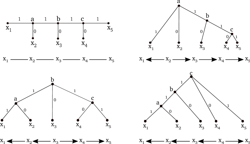
Figure 4: Placing the root. The tree $T$ in the upper left is the unique minimally resolved tree that explains $G(\mathrel{\overset{1}{\sim}})/\mathrel{\overset{0}{\sim}}$ (shown below $T$). Each of the tree inner vertices $a$, $b$, or $c$ of $T$ can be chosen as the root, giving rise to three distinct relations $\mathrel{\overset{1}{\rightharpoonup}}$. For the “siblings” in the unrooted tree $x_{1},x_{2}$ as well as $x_{4},x_{5}$ it holds that $x_{2}\mathrel{\overset{1}{\rightharpoonup}}x_{1}$ and $x_{4}\mathrel{\overset{1}{\rightharpoonup}}x_{5}$ for all three distinct relations. Thus, there are uniquely determined parts of $\mathrel{\overset{1}{\rightharpoonup}}$ conveyed by the information of $\mathrel{\overset{0}{\sim}}$ and $\mathrel{\overset{1}{\sim}}$ only.

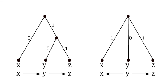
Figure 5: There are only two possibilities for induced connected subgraphs $H$ in $G(\mathrel{\overset{1}{\rightharpoonup}})/\mathrel{\overset{0}{\sim}}$ on three vertices, cf. Lemma 23, 24, and 25. Each of the distinct induced subgraphs imply a unique least resolved tree with a unique labeling.

Lemma 23.

In Case (i), the unique triple $\mathsf{yz|x}$ must be displayed by any tree $T(Q)$ that explains $Q$. Moreover, the paths $\mathbb{P}(u,v)$ and $\mathbb{P}(v,z)$ in $T(Q)$ contain both exactly one 1-edge, while the other paths $\mathbb{P}(u,x)$ and $\mathbb{P}(v,y)$ contain only 0-edges, where $u=\mathop{lca}(xy)=\mathop{lca}(xz)\neq\mathop{lca}(yz)=v$.

Proof.

Let $x,y,z\in V(Q)$ such that $xy,yz\in E$ and thus, $x\mathrel{\overset{1}{\rightharpoonup}}y\mathrel{\overset{1}{\rightharpoonup}}z$. Notice first that there must be two distinct last common ancestors for pairs of the three vertices $x,y,z$; otherwise, if $u=\mathop{lca}(xy)=\mathop{lca}(xz)=\mathop{lca}(yz)$, then the path $\mathbb{P}(uy)$ contains a 1-edge (since $x\mathrel{\overset{1}{\rightharpoonup}}y$) and hence $y\mathrel{\overset{1}{\rightharpoonup}}z$ is impossible. We continue to show that $u=\mathop{lca}(xy)=\mathop{lca}(xz)$. Assume that $u=\mathop{lca}(xy)\neq\mathop{lca}(xz)$. Hence, either the triple $\mathsf{xz|y}$ or $\mathsf{xy|z}$ is displayed by $T(Q)$. In either case the path $\mathbb{P}(u,y)$ contains a 1-edge, since $x\mathrel{\overset{1}{\rightharpoonup}}y$. This, however, implies $y\not\mathrel{\overset{1}{\rightharpoonup}}z$, a contradiction. Thus, $u=\mathop{lca}(xy)=\mathop{lca}(xz)$. Since there are two distinct last common ancestors, we have $u\neq v=\mathop{lca}(yz)$. Therefore, the triple $\mathsf{yz|x}$ must be displayed by $T(Q)$. From $y\mathrel{\overset{1}{\rightharpoonup}}z$ we know that $\mathbb{P}(v,y)$ only contains 0-edges and $\mathbb{P}(v,z)$ contains exactly one 1-edge; $x\mathrel{\overset{1}{\rightharpoonup}}y$ implies that $\mathbb{P}(x,u)$ contains only 0-edges. Moreover, since $\mathbb{P}(x,y)=\mathbb{P}(x,u)\cup\mathbb{P}(u,v)\cup\mathbb{P}(v,y)$ and $x\mathrel{\overset{1}{\rightharpoonup}}y$, the path $\mathbb{P}(u,v)$ must contain exactly one 1-edge. ∎

Lemma 24.

In Case (ii), there is a unique tree on the three vertices $x,y,z$ with single root $\rho$ displayed by any least resolved tree $T(Q)$ that explains $Q$. Moreover, the path $\mathbb{P}(\rho,y)$ contains only 0-edges, while the other paths $\mathbb{P}(\rho,x)$ and $\mathbb{P}(\rho,z)$ must both contain exactly one 1-edge.

Proof.

Assume for contradiction that there is a least resolved tree $T(Q)$ that displays $\mathsf{xy|z}$, $\mathsf{yz|x}$, or $\mathsf{xz|y}$.

The choice of $\mathsf{xy|z}$ implies $u=\mathop{lca}(xy)\neq\mathop{lca}(xz)=\mathop{lca}(yz)=v$. Since $y\mathrel{\overset{1}{\rightharpoonup}}x$ and $y\mathrel{\overset{1}{\rightharpoonup}}z$, $\mathbb{P}(v,y)\subsetneq\mathbb{P}(u,y)$ contain only 0-edges, while $\mathbb{P}(u,x)$ and $\mathbb{P}(v,z)$ each must contain exactly one 1-edge, respectively. This leads to a tree $T^{\prime}$ that yields the correct $\mathrel{\overset{1}{\rightharpoonup}}$-relation. However, this tree is not least resolved. By contracting the path $\mathbb{P}(u,v)$ to a single vertex $\rho$ and maintaining the labels on $\mathbb{P}(\rho,x)$, $\mathbb{P}(\rho,y)$, and $\mathbb{P}(\rho,z)$ we obtain the desired labeled least resolved tree with single root.

For the triple $\mathsf{yz|x}$ the existence of the unique, but not least resolved tree can be shown by the same argument with exchanged roles of $x$ and $y$.

For the triple $\mathsf{xz|y}$ we $u=\mathop{lca}(xy)=\mathop{lca}(yz)\neq\mathop{lca}(xz)=v$. From $y\mathrel{\overset{1}{\rightharpoonup}}x$ and $y\mathrel{\overset{1}{\rightharpoonup}}z$ we see that both paths $\mathbb{P}(u,x)=\mathbb{P}(u,v)\cup\mathbb{P}(v,x)$ and $\mathbb{P}(u,z)=\mathbb{P}(u,v)\cup\mathbb{P}(v,z)$ contain exactly one 1-edge, while all edges in $\mathbb{P}(u,y)$ are labeled $0$. There are two cases: (1) The path $\mathbb{P}(u,v)$ contains this 1-edge, which implies that both paths $\mathbb{P}(v,x)$ and $\mathbb{P}(v,z)$ contain only 0-edges. But then $x\mathrel{\overset{0}{\sim}}z$, a contradiction to $\mathrel{\overset{0}{\sim}}$ being discrete. (2) The path $\mathbb{P}(u,v)$ contains only 0-edges, which implies that each of the paths $\mathbb{P}(v,x)$ and $\mathbb{P}(v,z)$ contain exactly one 1-edge. Again, this leads to a tree that yields the correct $\mathrel{\overset{1}{\rightharpoonup}}$-relation, but it is not least resolved. By contracting the path $\mathbb{P}(u,v)$ to a single vertex $\rho$ and maintaining the labels on $\mathbb{P}(\rho,x)$, $\mathbb{P}(\rho,y)$, and $\mathbb{P}(\rho,z)$ we obtain the desired labeled least resolved tree with single root. ∎

Lemma 25.

Case (iii) cannot occur.

Proof.

Let $x,y,z\in V(Q)$ such that $xy,zy\in E$ and thus, $x\mathrel{\overset{1}{\rightharpoonup}}y$ and $z\mathrel{\overset{1}{\rightharpoonup}}y$. Hence, in the rooted tree that explains this relationship we have the following situation: All edges along $\mathbb{P}(u,x)$ are labeled $0$; exactly one edge along $\mathbb{P}(u,y)$ is labeled $1$, where $u=\mathop{lca}(x,y)$; all edges along $\mathbb{P}(v,z)$ are labeled $0$, and exactly one edge along $\mathbb{P}(v,y)$ is labeled $1$, where $v=\mathop{lca}(y,z)$. Clearly, $\mathop{lca}(x,y,z)\in\{u,v\}$. If $u=v$, then all edges in $\mathbb{P}(u,x)$ and $\mathbb{P}(u,z)$ are labeled $0$, implying that $x\mathrel{\overset{0}{\sim}}y$, contradicting that $\mathrel{\overset{0}{\sim}}$ is discrete.

Now assume that $u=\mathop{lca}(x,y)\neq v=\mathop{lca}(y,z)$. Hence, one of the triples $\mathsf{xy|z}$ or $\mathsf{yz|x}$ must be displayed by $T(Q)$. W.l.o.g., we can assume that $\mathsf{yz|x}$ is displayed, since the case $\mathsf{xy|z}$ is shown analogously by interchanging the role of $x$ and $z$. Thus, $\mathop{lca}(x,y,z)=\mathop{lca}(x,y)=u\neq\mathop{lca}(yz)=v$. Hence, $\mathbb{P}(u,y)=\mathbb{P}(u,v)\cup\mathbb{P}(v,y)$. Since $z\mathrel{\overset{1}{\rightharpoonup}}y$, the path $\mathbb{P}(v,y)$ contains a single 1-edge and $\mathbb{P}(v,z)$ contains only 0-edges. Therefore, the paths $\mathbb{P}(u,x)$ and $\mathbb{P}(u,v)$ contain only 0-edges, since $x\mathrel{\overset{1}{\sim}}y$. Since $\mathbb{P}(x,z)=\mathbb{P}(x,u)\cup\mathbb{P}(u,v)\cup\mathbb{P}(v,z)$ and all edges along $\mathbb{P}(u,x)$, $\mathbb{P}(u,v)$ and $\mathbb{P}(v,z)$ are labeled $0$, we obtain $x\mathrel{\overset{0}{\sim}}z$, again a contradiction. ∎

Taken together, we obtain the following immediate implication:

Corollary 26.

The graph $G(\mathrel{\overset{1}{\rightharpoonup}})/\mathrel{\overset{0}{\sim}}$ does not contain a pair of edges of the form $xv$ and $yv$.

Recall that the connected components $\underline{Q}$ in $G(\mathrel{\overset{1}{\rightharpoonup}})/\mathrel{\overset{0}{\sim}}$ are trees. By Cor. 26, $Q$ must be composed of distinct paths that “point away” from each other. In other words, let $P$ and $P^{\prime}$ be distinct directed path in $Q$ that share a vertex $v$, then it is never the case that there is an edge $xv$ in $P$ and an edge $yv$ in $P^{\prime}$, that is, both edges “pointing” to the same vertex $v$. We first consider directed paths in isolation.

Lemma 27.

Let $Q$ be a connected component in $G(\mathrel{\overset{1}{\rightharpoonup}})/\mathrel{\overset{0}{\sim}}$ that is a directed path with $n\geq 3$ vertices labeled $x_{1},\dots,x_{n}$ such that $x_{i}x_{i+1}\in E(Q)$, $1\leq i\leq n-1$. Then the tree $T(Q)$ explaining $Q$ must display all triples in $\mathcal{R}_{Q}=\{\mathsf{x_{i}x_{j}|x_{l}}\mid i,j>l\geq 1\}$. Hence, $T(Q)$ must display $\binom{n}{3}$ triples and is therefore the unique (least resolved) binary rooted tree $(\dots(x_{n},x_{n-1})x_{n-2})\dots)x_{2})x_{1}$ that explains $Q$. Moreover, all interior edges in $T(Q)$ and the edge incident to $x_{n}$ are labeled $1$ while all other edges are labeled $0$.

Proof.

Let $Q$ be a directed path as specified in the lemma. We prove the statement by induction. For $n=3$ the statement follows from Lemma 23. Assume the statement is true for $n=k$. Let $Q$ be a directed path with vertices $x_{1},\dots,x_{k},x_{k+1}$ and edges $x_{i}x_{i+1}$, $1\leq i\leq k$ and let $T(Q)$ be a tree that explains $Q$. For the subpath $Q^{\prime}$ on the vertices $x_{2},\dots,x_{k+1}$ we can apply the induction hypothesis and conclude that $T(Q^{\prime})$ must display the triples $\mathsf{x_{i}x_{j}|x_{l}}$ with $i,j>l\geq 2$ and that all interior edges in $T(Q^{\prime})$ and the edge incident to $x_{k+1}$ are labeled $1$ while all other edges are labeled $0$. Since $T(Q)$ must explain in particular the subpath $Q^{\prime}$ and since $T(Q^{\prime})$ is fully resolved, we can conclude that $T(Q^{\prime})$ is displayed by $T(Q)$ and that all edges in $T(Q)$ that are also in $T(Q^{\prime})$ retain the same label as in $T(Q^{\prime})$ .

Thus $T(Q)$ displays in particular the triples $\mathsf{x_{i}x_{j}|x_{l}}$ with $i,j>l\geq 2$. By Lemma 23, and because there are edges $x_{1}x_{2}$ and $x_{2}x_{3}$, we see that $T(Q)$ must also display $\mathsf{x_{2}x_{3}|x_{1}}$. Take any triple $\mathsf{x_{3}x_{j}|x_{2}}$, $j>3$. Application of the triple-inference rules shows that any tree that displays $\mathsf{x_{2}x_{3}|x_{1}}$ and $\mathsf{x_{3}x_{j}|x_{2}}$ must also display $\mathsf{x_{2}x_{j}|x_{1}}$ and $\mathsf{x_{3}x_{j}|x_{1}}$. Hence, $T(Q)$ must display these triples. Now we apply the same argument to the triples $\mathsf{x_{2}x_{j}|x_{1}}$ and $\mathsf{x_{i}x_{j}|x_{2}}$, $i,j>2$ and conclude that in particular, the triple $\mathsf{x_{i}x_{j}|x_{1}}$ must be displayed by $T(Q)$ and thus, the the entire set of triples $\{\mathsf{x_{i}x_{j}|x_{l}}\colon i,j>l\geq 1\}$. Hence, there are $\binom{n}{3}$ triples and thus, the set of triples that needs to be displayed by $T(Q)$ is strictly dense. Making use of a technical result from (Hellmuth et al., 2015, Suppl. Material), we obtain that $T(Q)$ is the unique binary tree $(\dots(x_{n},x_{n-1})x_{n-2})\dots)x_{2})x_{1}$. Now it is an easy exercise to verify that the remaining edge containing $x_{1}$ must be labeled $0$, while the interior edge not contained in $T(Q^{\prime})$ must all be 1-edges. ∎

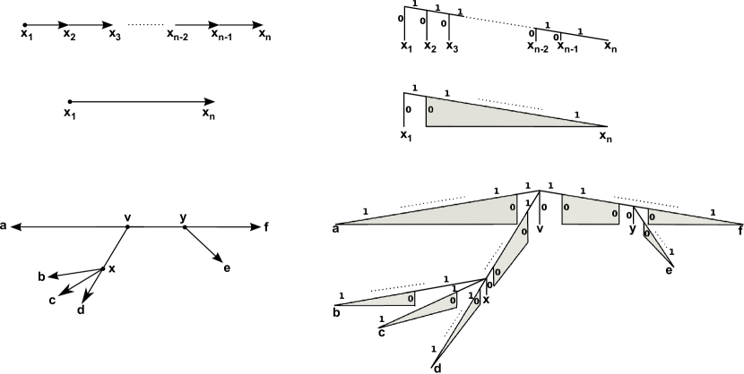
Figure 6: Connected components $Q$ in $G(\mathrel{\overset{1}{\rightharpoonup}})/\mathrel{\overset{0}{\sim}}$ are trees composed of paths pointing away from each other. On the top, a directed path $\mathbb{P}(x_{1},x_{n})$ together with its unique least resolved tree representation is shown. In the middle, an abstract picture of the path $\mathbb{P}(x_{1},x_{n})$ and its tree is given. Bottom, a larger example of a connected component $Q$ in $G(\mathrel{\overset{1}{\rightharpoonup}})/\mathrel{\overset{0}{\sim}}$ and its tree-representation are sketched.

If $Q$ is connected but not a simple path, it is a tree composed of the paths pointing away from each other as shown in Fig. 6. It remains to show how to connect the distinct trees that explain these paths to obtain a tree $T(Q)$ for $Q$. To this end, we show first that there is a unique vertex $v$ in $Q$ such that no edge ends in $v$.

Lemma 28.

Let $Q$ be a connected component in $G(\mathrel{\overset{1}{\rightharpoonup}})/\mathrel{\overset{0}{\sim}}$. Then there is a unique vertex $v$ in $Q$ such that there is no edge $xv\in E(Q)$.

Proof.

Corollary 26 implies that for each vertex $v$ in $Q$ there is at most one edge $xv\in E(Q)$. If for all vertices $w$ in $Q$ we would have an edge $xw\in E(Q)$, then $Q$ contains cycles, contradicting the tree structure of $Q$. Hence, there is at least one vertex $v$ so that there is no edge of the form $xv\in E(Q)$. Assume there are two vertices $v,v^{\prime}$ so that there are no edges of the form $xv,yv^{\prime}$, then all edges incident to $v,v^{\prime}$ are of the form $vx,v^{\prime}y$. However, in this case, the unique path connecting $v,v^{\prime}$ in $Q$ must contain two edges of the form $aw$, $bw$; a contradiction to Corollary 26. Thus, there is exactly one vertex $v$ in $Q$ such that there is no edge $xv\in E(Q)$. ∎

By Lemma 28, for each connected component $Q$ of $G(\mathrel{\overset{1}{\rightharpoonup}})/\mathrel{\overset{0}{\sim}}$ there is a unique vertex $v_{Q}$ s.t. all edges incident to $v_{Q}$ are of the form $v_{Q}x$. That is, all directed paths that are maximal w.r.t. inclusion start in $v_{Q}$. Let $\mathcal{P}_{Q}$ denote the sets of all such maximal paths. Thus, for each path $P\in\mathcal{P}_{Q}$ there is the triple set $\mathcal{R}_{P}$ according to Lemma 27 that must be displayed by any tree that explains also $Q$. Therefore, $T(Q)$ must display all triples in $\mathcal{R}_{Q}=\cup_{P\in\mathcal{P}_{Q}}\mathcal{R}_{P}$.

The underlying undirected graph $\underline{G(\mathrel{\overset{1}{\rightharpoonup}})/\mathrel{\overset{0}{\sim}}}$ is isomorphic to $G(\mathrel{\overset{1}{\sim}})/\mathrel{\overset{0}{\sim}}$. Thus, with Algorithm 1, one can similar to the unrooted case, first construct the tree $T(\underline{Q})$ and then set the root $\rho_{Q}=v^{\prime}_{Q}$ to obtain $T(Q)$. It is easy to verify that this tree $T(Q)$ displays all triples in $\mathcal{R}_{Q}$. Moreover, any edge-contradiction in $T(Q)$ leads to the loss of an input triple $\mathcal{R}_{Q}$ and in particular, to a wrong pair of vertices w.r.t. $\mathrel{\overset{1}{\rightharpoonup}}$ or $\mathrel{\overset{0}{\sim}}$. Thus, $T(Q)$ is a least resolved tree for $\mathcal{R}_{Q}$ and therefore, a least resolved tree that explains $Q$.

We summarize these arguments in

Corollary 29.

Let $Q$ be a connected component in $G(\mathrel{\overset{1}{\rightharpoonup}})/\mathrel{\overset{0}{\sim}}$. Then a tree $T(Q)$ that explains $Q$ can be obtained from the unique minimally resolved tree $T(\underline{Q})$ that explains $\underline{Q}$ by choosing the unique vertex $v$ where all edges incident to $v$ are of the form $vx$ as the root $\rho_{Q}$.

If $G(\mathrel{\overset{1}{\rightharpoonup}})/\mathrel{\overset{0}{\sim}}$ is disconnected, one can apply Algorithm 2, to obtain the tree $T(G(\mathrel{\overset{1}{\sim}})/\mathrel{\overset{0}{\sim}})$ and then chose either one of the vertices $\rho_{Q}$ or the vertex $z_{T}$ as root to obtain $T(G(\mathrel{\overset{1}{\rightharpoonup}})/\mathrel{\overset{0}{\sim}})$, in which case all triples of $\mathcal{R}_{G(\mathrel{\overset{1}{\rightharpoonup}})/\mathrel{\overset{0}{\sim}}}=\cup_{Q}\mathcal{R}_{Q}$ are displayed. Again, it is easy to verify that any edge-contradiction leads to a wrong pair of vertices in $\mathrel{\overset{1}{\rightharpoonup}}$ or $\mathrel{\overset{0}{\sim}}$. Thus, $T(G(\mathrel{\overset{1}{\rightharpoonup}})/\mathrel{\overset{0}{\sim}})$ is a least resolved tree for $\mathcal{R}_{G(\mathrel{\overset{1}{\rightharpoonup}})/\mathrel{\overset{0}{\sim}}}$.

To obtain uniqueness of minimally resolved trees one can apply similar arguments as in the proofs of Theorems 15 and 17. This yields the following characterization:

Theorem 30.

Let $Q_{1},\dots Q_{k}$ be the connected components in $G(\mathrel{\overset{1}{\rightharpoonup}})/\mathrel{\overset{0}{\sim}}$. Up to the choice of the vertices $q^{\prime}_{i}$ in Line 11 of Alg. 2 for the construction of $T(\underline{Q_{i}})$ and the choice of the root $\rho\in\{\rho_{Q_{1}},\ldots\rho_{Q_{k}},z\}$, the tree $T^{*}=T(G(\mathrel{\overset{1}{\rightharpoonup}})/\mathrel{\overset{0}{\sim}}))$ is the unique minimally resolved tree that explains $G(\mathrel{\overset{1}{\rightharpoonup}})/\mathrel{\overset{0}{\sim}}$.

6 Mix of symmetric and anti-symmetric relations

In real data, e.g., in the application to mitochondrial genome arrangements, one can expect that the known relationships are in part directed and in part undirected. Such data are naturally encoded by a relation $\mathrel{\overset{1}{\rightharpoonup}}$ with directional information and a relation $\mathrel{\overset{1\star}{\sim}}$ comprising the set of pairs for which it is unknown whether one of $x\mathrel{\overset{1}{\rightharpoonup}}y$ and $y\mathrel{\overset{1}{\rightharpoonup}}x$ or $x\mathrel{\overset{1}{\sim}}y$ are true. Here, $\mathrel{\overset{1}{\sim}}$ is a subset of $\mathrel{\overset{1\star}{\sim}}$. The disjoint union $\mathrel{\overset{1\star}{\sim}}\uplus\mathrel{\overset{1}{\rightharpoonup}}$ of these two parts can be seen as refinement of a corresponding symmetrized relation $x\mathrel{\overset{1}{\sim}}y$. Ignoring the directional information one can still construct the tree $T(G(\mathrel{\overset{1}{\sim}})/\mathrel{\overset{0}{\sim}})$. In general there will be less information of the placement of the root in $T(G(\mathrel{\overset{1\star}{\sim}}\cup\mathrel{\overset{1}{\rightharpoonup}})/\mathrel{\overset{0}{\sim}})$ than with a fully directed edge set.

In what follows, we will consider all edges of $G(\mathrel{\overset{1\star}{\sim}}\cup\mathrel{\overset{1}{\rightharpoonup}})/\mathrel{\overset{0}{\sim}}$ to be directed, that is, for a symmetric pair $(a,b)\in\mathrel{\overset{1\star}{\sim}}$ we assume that both directed edges $ab$ and $ba$ are contained in $G(\mathrel{\overset{1\star}{\sim}}\cup\mathrel{\overset{1}{\rightharpoonup}})/\mathrel{\overset{0}{\sim}}$. Still, for any connected component $Q$ the underlying undirected graph $\underline{Q}$ is a tree. Given a component $Q$ we say that a directed edge $xy\in E(Q)$ points away from the vertex $v$ if the unique path in $\underline{Q}$ from $v$ to $x$ does not contain $y$. In this case the path from $v$ to $y$ must contain $x$. Note that in this way we defined “pointing away from $v$” not only for the edges incident to $v$, but for all directed edges. A vertex $v$ is a central vertex if, for any two distinct vertices $x,y\in V$ that form an edge in $T$, either $xy$ or $yx$ in $T$ points away from $v$.

As an example consider the tree $a\leftarrow b\rightarrow c\leftrightarrow d\rightarrow e$. There is only the edge $bc$ containing $b$ and $c$. However, $bc$ does not point away from vertex $d$, since the unique path from $d$ to $b$ contains $c$. Thus $d$ is not central. On the other hand, $b$ is a central vertex. The only possibility in this example to obtain a valid relation $\mathrel{\overset{1}{\rightharpoonup}}$ that can be displayed by rooted 0/1-edge-labeled tree is provided by removing the edge $dc$, since otherwise Cor. 26 would be violated.

In the following, for given relations $\mathrel{\overset{1\star}{\sim}}$ and $\mathrel{\overset{1}{\rightharpoonup}}$ we will denote with $\mathrel{\overset{1\star}{\rightharpoonup}}$ a relation that contains $\mathrel{\overset{1}{\rightharpoonup}}$ and exactly one pair, either $(x,y)$ or $(y,x)$, from $\mathrel{\overset{1\star}{\sim}}$.

Lemma 31.

For a given graph $G(\mathrel{\overset{1\star}{\sim}}\cup\mathrel{\overset{1}{\rightharpoonup}})/\mathrel{\overset{0}{\sim}}$ the following statements are equivalent:

• There is a relation $\mathrel{\overset{1\star}{\rightharpoonup}}$ that is the antisymmetric single-1-relation of some 0/1-edge-labeled tree.

• There is a central vertex in each connected component $Q$ of $G(\mathrel{\overset{1\star}{\sim}}\cup\mathrel{\overset{1}{\rightharpoonup}})/\mathrel{\overset{0}{\sim}}$.

Proof.

If there is a relation $\mathrel{\overset{1\star}{\rightharpoonup}}$ that can be displayed by a rooted 0/1-edge-labeled tree, then $G(\mathrel{\overset{1\star}{\rightharpoonup}})/\mathrel{\overset{0}{\sim}}$ consists of connected components $Q$ where each connected component is a tree composed of maximal directed paths that point away from each other. Hence, for each connected component $Q$ there is the unique vertex $v_{Q}$ such that all edges incident to $v_{Q}$ are of the form $v_{Q}x$ and, in particular, $v_{Q}$ is a central vertex $v_{Q}$ in $Q$ and thus, in $G(\mathrel{\overset{1\star}{\sim}}\cup\mathrel{\overset{1}{\rightharpoonup}})/\mathrel{\overset{0}{\sim}}$.

Conversely, assume that each connected component $Q$ has a central vertex $v_{Q}$. Hence, one can remove all edges that do not point away from $v_{Q}$ and hence obtain a connected component $Q^{\prime}$ that is still a tree with $V(Q)=V(Q^{\prime})$ so that all maximal directed paths point away from each other and in particular, start in $v_{Q}$. Thus, for the central vertex $v_{Q}$ all edges incident to $v_{Q}$ are of the form $v_{Q}x$. Since $Q^{\prime}$ is now a connected component in $G(\mathrel{\overset{1\star}{\rightharpoonup}})/\mathrel{\overset{0}{\sim}}$, we can apply Cor. 29 to obtain the tree $T(Q^{\prime})$ and Thm. 30 to obtain $T(G(\mathrel{\overset{1\star}{\rightharpoonup}})/\mathrel{\overset{0}{\sim}})$. ∎

The key consequence of this result is the following characterization of the constraints on the possible placements of the root.

Corollary 32.

Let $Q$ be a connected component in $G(\mathrel{\overset{1\star}{\sim}}\cup\mathrel{\overset{1}{\rightharpoonup}})/\mathrel{\overset{0}{\sim}}$ and let $T(\underline{Q})$ be the unique least resolved tree that explains the underlying undirected graph $\underline{Q}$. Then each copy $v^{\prime}$ of a vertex $v$ in $Q$ can be chosen to be the root in $T(\underline{Q})$ to obtain $T(Q)$ if and only if $v$ is a central vertex in $Q$.

7 Concluding Remarks

In this contribution we have introduced a class of binary relations deriving in a natural way from edge-labeled trees. This construction has been inspired by the conceptually similar class of relations induced by vertex-labeled trees (Hellmuth and Wieseke, 2017). The latter have co-graph structure and are closely related to orthology and paralogy (Hellmuth et al., 2013; Lafond and El-Mabrouk, 2014; Hellmuth et al., 2015; Hellmuth and Wieseke, 2015). Defining $x\sim y$ whenever at least one 1-edge lies along the path from $x$ to $y$ is related to the notion of xenology: the edges labeled 1 correspond to horizontal gene transfer events, while the 0-edge encode vertical transmission. In its simplest setting, this idea can also be combined with vertex labels, leading to the directed analog of co-graphs (Hellmuth et al., 2016). Here, we have explored an even simpler special case: the existence of a single 1-label along the connecting path, which captures the structure of rare event data as we have discussed in the introduction. We have succeeded here in giving a complete characterization of the relationships between admissible relations, which turned out to be forests, and the underlying phylogenetic tree. Moreover, for all such cases we gave polynomial-time algorithms to compute the trees explaining the respective relation.

The characterization of single-1 relations is of immediate relevance for the use of rare events in molecular phylogenetics. In particular, it determines lower bounds on the required data: if too few events are known, many taxa remain in $\mathrel{\overset{0}{\sim}}$ relation and thus unresolved. On the other hand, if taxa are spread too unevenly, $G(\mathrel{\overset{1}{\rightharpoonup}})/\mathrel{\overset{0}{\sim}}$ will be disconnected, consisting of connected components separated by multiple events. The approach discussed here, of course, is of practical use only if the available event data are very sparse. If taxa are typically separated by multiple events, classical phylogenetic approaches, i.e., maximum parsimony, maximum likelihood, or Bayesian methods, will certainly be preferable. An advantage of using the single-1 relation is that it does not require the product structure of independent characters implicit in the usual, sequence or character-based methods, nor does it require any knowledge of the algebraic properties of the underlying operations as, e.g., in phylogenetic reconstruction from (mitochondrial) gene order rearrangements. This begs the question under which conditions on the input data identical results are obtained from the direct translation of the single-1 relation and maximum parsimony on character data or break point methods for genome rearrangments.

A potentially useful practical application of our results is a new strategy to incorporate rare event data into conventional phylogenetic approaches. Trees obtained from a single-1 relation will in general be poorly resolved. Nevertheless, they determine some monophyletic groups (in the directed case) or a set of split (in the undirected case) that have to be present in the true phylogeny. Many of the software tools commonly used in molecular phylogenetic can incorporate this type of constraints. Assuming the there is good evidence that the rare events are homoplasy-free, the $T(G(\mathrel{\overset{1}{\rightharpoonup}})/\mathrel{\overset{0}{\sim}})$ represents the complete information from the rare events that can be used constrain the tree reconstruction process.

The analysis presented here makes extensive use of the particular properties of the single-1 relation and hence does not seem to generalize easily to other interesting cases. Horizontal gene transfer, for example, is expressed naturally in terms of the “at-least-one-1” relation $\mathrel{\rightsquigarrow}$. It is worth noting that $\mathrel{\rightsquigarrow}$ also has properties (L1) and (L2) and hence behaves well w.r.t. contraction of the underlying tree and restriction to subsets of leaves. Whether this is sufficient to obtain a complete characterization remains an open question.

Several general questions arise naturally. For instance, is there a characterization of admissible relations in terms of forbidden subgraphs graphs or minors? For instance, the relation $\mathrel{\overset{1}{\rightharpoonup}}/\mathrel{\overset{0}{\sim}}$ is characterized in terms of the forbidden subgraph $x\rightarrow v\leftarrow y$. Hence, it would be of interest, whether such characterizations can be derived for arbitrary relations $\mathrel{\overset{k}{\rightharpoonup}}$ or for $\mathrel{\rightsquigarrow}$. If so, can these forbidden substructures be inferred in a rational manner from properties of vertex and/or edge labels along the connecting paths in the explaining tree? Is this the case at least for labels and predicates satisfying (L1) and (L2)?

References

- Abascal et al. (2012) Abascal F, Posada D, Zardoya R, 2012. The evolution of the mitochondrial genetic code in arthropods revisited. Mitochondrial DNA 23:84–91.
- Ashkenazy et al. (2014) Ashkenazy H, Cohen O, Pupko T, Huchon D, 2014. Indel reliability in indel-based phylogenetic inference. Genome Biol Evol 6:3199–3209.
- Bernt et al. (2007) Bernt M, Merkle D, Rasch K, Fritzsch G, Perseke M, Bernhard D, Schlegel M, Stadler PF, Middendorf M, 2007. CREx: Inferring genomic rearrangements based on common intervals. Bioinformatics 23:2957–2958.
- Boore (2006) Boore JL, 2006. The use of genome-level characters for phylogenetic reconstruction. Trends Ecol Evol 21:439–446.
- Boore and Brown (1998) Boore JL, Brown WM, 1998. Big trees from little genomes: mitochondrial gene order as a phylogenetic tool. Curr Opin Genet Dev 8:668–674.
- Brandstädt et al. (2010) Brandstädt A, Le VB, Rautenbach D, 2010. Exact leaf powers. Theoretical Computer Science 411:2968 – 2977.
- Bryant and Steel (1995) Bryant D, Steel M, 1995. Extension operations on sets of leaf-labelled trees. Adv Appl Math 16:425–453.
- Calamoneri et al. (2013) Calamoneri T, Montefusco E, Petreschi R, Sinaimeri B, 2013. Exploring pairwise compatibility graphs. Theoretical Computer Science 468:23 – 36.
- Calamoneri and Sinaimeri (2016) Calamoneri T, Sinaimeri B, 2016. Pairwise compatibility graphs: A survey. SIAM Review 58:445–460.
- Chaudhuri et al. (2006) Chaudhuri K, Chen K, Mihaescu R, Rao S, 2006. On the tandem duplication-random loss model of genome rearrangement. In: Proceedings of the 17th Annual ACM-SIAM Symposium on Discrete Algorithms, (pp. 564–570). ACM.
- Deeds et al. (2005) Deeds EJ, Hennessey H, Shakhnovich EI, 2005. Prokaryotic phylogenies inferred from protein structural domains. Genome Res 15:393–402.
- Dekker (1986) Dekker MCH, 1986. Reconstruction methods for derivation trees. Master’s thesis, Vrije Universiteit, Amsterdam, Netherlands.
- Donath and Stadler (2014) Donath A, Stadler PF, 2014. Molecular morphology: Higher order characters derivable from sequence information. In: Wägele JW, Bartolomaeus T, editors, Deep Metazoan Phylogeny: The Backbone of the Tree of Life. New insights from analyses of molecules, morphology, and theory of data analysis, chap. 25, (pp. 549–562). Berlin: de Gruyter.
- Durocher et al. (2013) Durocher S, Mondal D, Rahman MS, 2013. On graphs that are not PCGs. In: Ghosh SK, Tokuyama T, editors, WALCOM: Algorithms and Computation: 7th International Workshop, WALCOM 2013, Kharagpur, India, February 14-16, 2013. Proceedings, (pp. 310–321). Berlin, Heidelberg: Springer Berlin Heidelberg.
- Dutilh et al. (2008) Dutilh BE, Snel B, Ettema TJ, Huynen MA, 2008. Signature genes as a phylogenomic tool. Mol Biol Evol 25:1659–1667.
- Forst et al. (2006) Forst CV, Flamm C, Hofacker IL, Stadler PF, 2006. Algebraic comparison of metabolic networks, phylogenetic inference, and metabolic innovation. BMC Bioinformatics 7:67 [epub].
- Forst and Schulten (2001) Forst CV, Schulten K, 2001. Phylogenetic analysis of metabolic pathways. J Mol Evol 52:471–489.
- Fritzsch et al. (2006) Fritzsch G, Schlegel M, Stadler PF, 2006. Alignments of mitochondrial genome arrangements: Applications to metazoan phylogeny. J Theor Biol 240:511–520.
- Hartmann et al. (2016) Hartmann T, Chu AC, Middendorf M, Bernt M, 2016. Combinatorics of tandem duplication random loss mutations on circular genomes. IEEEACM Trans Comput Biol Bioinform .
- Hellmuth et al. (2013) Hellmuth M, Hernandez-Rosales M, Huber KT, Moulton V, Stadler PF, Wieseke N, 2013. Orthology relations, symbolic ultrametrics, and cographs. J Math Biol 66:399–420.
- Hellmuth et al. (2016) Hellmuth M, Stadler PF, Wieseke N, 2016. The mathematics of xenology: Di-cographs, symbolic ultrametrics, 2-structures and tree-representable systems of binary relations. J Math Biol In press; doi:10.1007/s00285-016-1084-3.
- Hellmuth and Wieseke (2015) Hellmuth M, Wieseke N, 2015. On symbolic ultrametrics, cotree representations, and cograph edge decompositions and partitions. In: Xu D, Du D, Du D, editors, Computing and Combinatorics, vol. 9198 of Lecture Notes Comp. Sci., (pp. 609–623). Springer International Publishing.
- Hellmuth and Wieseke (2016) Hellmuth M, Wieseke N, 2016. From sequence data including orthologs, paralogs, and xenologs to gene and species trees. In: Pontarotti P, editor, Evolutionary Biology: Convergent Evolution, Evolution of Complex Traits, Concepts and Methods, (pp. 373–392). Cham: Springer.
- Hellmuth and Wieseke (2017) Hellmuth M, Wieseke N, 2017. On tree representations of relations and graphs: symbolic ultrametrics and cograph edge decompositions. Journal of Combinatorial Optimization (pp. 1–26).
- Hellmuth et al. (2015) Hellmuth M, Wieseke N, Lechner M, Lenhof HP, Middendorf M, Stadler PF, 2015. Phylogenomics with paralogs. Proceedings of the National Academy of Sciences 112:2058–2063. DOI: 10.1073/pnas.1412770112.
- Hennig (1950) Hennig W, 1950. Grundzüge einer Theorie der Phylogenetischen Systematik. Berlin: Deutscher Zentralverlag.
- Hernandez-Rosales et al. (2012) Hernandez-Rosales M, Hellmuth M, Wieseke N, Huber KT, Moulton V, Stadler PF, 2012. From event-labeled gene trees to species trees. BMC Bioinformatics 13:S6.
- Krauss et al. (2008) Krauss V, Thümmler C, Georgi F, Lehmann J, Stadler PF, Eisenhardt C, 2008. Near intron positions are reliable phylogenetic markers: An application to Holometabolous Insects. Mol Biol Evol 25:821–830.
- Lafond and El-Mabrouk (2014) Lafond M, El-Mabrouk N, 2014. Orthology and paralogy constraints: satisfiability and consistency. BMC Genomics 15 S6:S12.
- Lavrov (2007) Lavrov DV, 2007. Key transitions in animal evolution: a mitochondrial DNA perspective. Integr Comp Biol 47:734–743.
- Mazurie et al. (2008) Mazurie A, Bonchev D, Schwikowski B, Buck GA, 2008. Phylogenetic distances are encoded in networks of interacting pathways. Bioinformatics 24:2579–2585.
- Mehnaz and Rahman (2013) Mehnaz S, Rahman MS, 2013. Pairwise compatibility graphs revisited. In: 2013 International Conference on Informatics, Electronics and Vision (ICIEV), (pp. 1–6).
- Misof and Fleck (2003) Misof B, Fleck G, 2003. Comparative analysis of mt LSU rRNA secondary structures of Odonates: structural variability and phylogenetic signal. Insect Mol Biol 12:535–47.
- Prohaska et al. (2004) Prohaska SJ, Fried C, Amemiya CT, Ruddle FH, Wagner GP, Stadler PF, 2004. The shark HoxN cluster is homologous to the human HoxD cluster. J Mol Evol (p. 58). 212-217.
- Rogozin et al. (2005) Rogozin IB, Sverdlov AV, Babenko VN, Koonin EV, 2005. Analysis of evolution of exon-intron structure of eukaryotic genes. Brief Bioinform 6:118–134.
- Rokas and Holland (2000) Rokas A, Holland PW, 2000. Rare genomic changes as a tool for phylogenetics. Trends Ecol Evol 15:454–459.
- Sankoff et al. (1992) Sankoff D, Leduc G, Antoine N, Paquin B, Lang BF, Cedergren R, 1992. Gene order comparisons for phylogenetic inference: Evolution of the mitochondrial genome. Proc Natl Acad Sci USA 89:6575–6579.
- Sempere et al. (2006) Sempere LF, Cole CN, McPeek MA, Peterson KJ, 2006. The phylogenetic distribution of metazoan microRNAs: insights into evolutionary complexity and constraint. J Exp Zoolog B Mol Dev Evol 306:575–588.
- Semple and Steel (2003) Semple C, Steel M, 2003. Phylogenetics, vol. 24 of Oxford Lecture Series in Mathematics and its Applications. Oxford: Oxford University Press.
- Shedlock and Okada (2000) Shedlock AM, Okada N, 2000. SINE insertions: powerful tools for molecular systematics. BioEssays 22:148–160.
- Simmons and Ochoterena (2000) Simmons MP, Ochoterena H, 2000. Gaps as characters in sequence-based phylogenetic analyses. Syst Biol 49:369–381.
- Stechmann and Cavalier-Smith (2003) Stechmann A, Cavalier-Smith T, 2003. The root of the eukaryote tree pinpointed. Curr Biol 13:R665–R666.
- Tang and Wang (2005) Tang J, Wang LS, 2005. Improving genome rearrangement phylogeny using sequence-style parsimony. In: Karypis G, Bourbakis NG, Tsai J, editors, Proceedings of the IEEE Fifth Symposium on Bioinformatics and Bioengineering (BIBE’05), (pp. 137–144). Los Alamitos, CA: IEEE Computer Society.
- Wagner and Stadler (2003) Wagner G, Stadler PF, 2003. Quasi-independence, homology and the unity of type: A topological theory of characters. J Theor Biol 220:505–527.
- Wang et al. (2006) Wang LS, Warnow T, Moret BM, Jansen RK, , Raubeson LA, 2006. Distance-based genome rearrangement phylogeny. J Mol Evol 63:473–483.
- Yang et al. (2005) Yang S, Doolittle RF, Bourne PE, 2005. Phylogeny determined by protein domain content. Proc Natl Acad Sci USA 102:373–378.
- Yanhaona et al. (2010) Yanhaona MN, Bayzid MS, Rahman MS, 2010. Discovering pairwise compatibility graphs. In: Thai MT, Sahni S, editors, Computing and Combinatorics: 16th Annual International Conference, COCOON 2010, Nha Trang, Vietnam, July 19-21, 2010. Proceedings, (pp. 399–408). Berlin, Heidelberg: Springer Berlin Heidelberg.
- Yanhaona et al. (2008) Yanhaona MN, Hossain KSMT, Rahman MS, 2008. Pairwise compatibility graphs. In: Nakano Si, Rahman MS, editors, WALCOM: Algorithms and Computation: Second International Workshop, WALCOM 2008, Dhaka, Bangladesh, February 7-8, 2008. Proceedings, (pp. 222–233). Berlin, Heidelberg: Springer Berlin Heidelberg.