Nonperturbative QED vacuum birefringence

Abstract

In this paper we represent nonperturbative calculation for one-loop Quantum Electrodynamics (QED) vacuum birefringence in presence of strong magnetic field. The dispersion relations for electromagnetic wave propagating in strong magnetic field point to retention of vacuum birefringence even in case when the field strength greatly exceeds Sauter-Schwinger limit. This gives a possibility to extend some predictions of perturbative QED such as electromagnetic waves delay in pulsars neighbourhood or wave polarization state changing (tested in PVLAS) to arbitrary magnetic field values. Such expansion is especially important in astrophysics because magnetic fields of some pulsars and magnetars greatly exceed quantum magnetic field limit, so the estimates of perturbative QED effects in this case require clarification.

1 Introduction

From the very beginning, radiative corrections to the QED Lagrangian coming from the vacuum fluctuations have been the subject of a great interest. Such corrections, accounted on background of constant and homogeneous electromagnetic field, lead to Heisenberg-Euler effective Lagrangian a1 . The scale parameter for nonlinearities in Heisenberg-Euler electrodynamics (characteristic quantum electrodynamic induction or Schwinger limit for electric field) $B_{c}=E_{c}=m^{2}c^{3}/e\hbar=4.41\cdot 10^{13}$G distinguishes different regimes of the theory.

The perturbative or post-Maxwellian regime takes place for most of the available in contemporary laboratory electromagnetic fields $E,B\ll E_{c},B_{c}$. In this case the Heisenberg-Euler Lagrangian can be expanded in power series of electromagnetic field tensor invariants. The perturbative regime of QED is well understood and many of its predictions have been experimentally observed. For instance, electron anomalous magnetic moment remains a great example of unprecedented correspondence between theoretical and experimental results a2 ; a3 . Some other predictions such as the Delbrück scattering a4 , Lamb shift a5 and photon splitting a6 ; a7 are also well-established. Another manifestation of perturbative QED lies in the phenomenon of vacuum behavior like a polarizable medium with the cubic nonlinearity in constitutive relations. Such semiclassical description leads to birefringence of electromagnetic waves in vacuum in presence of external field. The attempt of vacuum birefringence experimental observation was made in PVLAS experiment a8 ; a9 . The measurement of refractive indexes induced by vacuum birefringence was based on detecting rotation of electromagnetic wave polarization when it propagated in dipole magnetic field with induction $B_{ext}=2.5\cdot 10^{4}$G. The results of PVLAS set a new limit on vacuum magnetic birefringence above the level pointed out by QED a10 ; a9 . According to the authors, the discrepancy can be explained beyond the Standard Model by interaction with axiones. The experiment also bounded the coupling constant of axion-like particles and photons a10 ; a9 . Since the vacuum birefringence is a very small macroscopic quantum effect it’s detection needs strong enough magnetic field source, which is difficult to obtain in laboratory. At the same time, usage of compact astrophysical objects as natural magnetic fields sources provides wide opportunities for vacuum birefringence investigation due to the fact that for many pulsars and manetars the magnetic field is close to or even exceeds $B_{c}$. Vacuum birefringence in this case can be detected by measuring X- and gamma- ray polarization passing the region of the strong magnetic field near the pulsar. Due to the difference in wave propagation velocities induced by vacuum birefringence the time lag between the arrival of the fast and the slow mode to the detector is proportional to vacuum refractive index difference for each polarization mode. The calculations in perturbative QED regime show the detectability of the effect a11 and give the value for the time lag $\Delta t\sim 10^{-7}$s. The results of calculations are valid when the pulsar field $B<B_{c}$, however the existence of pulsars with the overcritical field (for instance B1509-58 with the $B\sim 1.5\cdot 10^{14}$G) provides an attractive possibility to enhance the estimates for the time lag. Such calculations require of vacuum birefringence consideration outside the perturbative regime.

Nonperturbative regime of QED arises when we consider external fields which values are close to or exceed the scale parameter of the Heisenberg-Euler electrodynamics $E,B\sim E_{c},B_{c}$. This regime shows one of the most amazing properties – vacuum instability due to electron-positron pair production. The effect is expected a14 when the electric field exceeds so-called Schwinger limit $E>E_{c}$ and, although it has never been observed directly, the advances of high-intensity laser physics and implementation of such projects as ELI, XFEL and others a12 ; a13 give a great promise in this area. In general, QED in nonperturbative regime is poorly investigated and provides new challenges both in theoretical and experimental research.

In this paper we will focus on one-loop QED vacuum birefringence in nonperturbative regime. In addition to entirely quantum technic proposed in a15 ; a16 , we represent a semiclassical approach. The maim aim of our research is to expand vacuum birefringence predictions for different experiments to values of strong magnetic fields close to character quantum electrodynamic induction. The paper is organized as follows: in Sec.2 we derive constitutive relations for QED, Sec.3 is devoted to the weak electromagnetic wave propagation in strong magnetic field, in Sec.4 we discuss QED birefringence expansion following from obtained dispersion relations and possibilities for it’s observation and in conclusive Sec.5 we summarize our results.

2 Constitutive relations for nonperturbative QED

The Lagrangian in QED is represented as a series of corrections to Maxwell electrodynamics. One-loop QED considers only the first non-vanishing correction which in non-perturbative regime has the following form b1 :

$$L_{1}=-{\alpha B_{c}^{2}\over 8\pi^{2}}\int\limits_{0}^{\infty}{e^{-s}\over s^{3}}\Big{[}sa\ \cot(sa)\cdot sb\ \coth(sb)-1-{s^{2}\over 3}(b^{2}-a^{2})\Big{]}ds,$$ (1)

where $\alpha=e^{2}/\hbar c$ – is a fine structure constant and the parameters $a$ and $b$ are expressed by the electromagnetic field components:

$$a=-{i\over\sqrt{2}B_{c}}\Big{(}\sqrt{F+iG}-\sqrt{F-iG}\Big{)},\quad b={1\over\sqrt{2}B_{c}}\Big{(}\sqrt{F+iG}+\sqrt{F-iG}\Big{)},$$ (2)

where the notations $F=({\bf B}^{2}-{\bf E}^{2})/2$ and $G=({\bf E}{\bf B})$ were used for brevity. Strictly speaking, the Heisenberg-Euler Lagrange function is valid only in case of constant and homogeneous background fields, at least at the typical scale of Compton wavelength $\lambda_{c}=h/mc$. Also it should be noted that the auxiliary parameters $a$ and $b$ of Heisenberg-Euler Lagrangian (1) are special because $\pm a$ and $\pm b$ are the eigenvalues of the electromagnetic field tensor $F_{ik}$ when field value is constant and this makes the problem of QED radiative corrections exactly solvable arx1 .

In semiclassical approach Heisenberg-Euler theory can be interpreted as nonlinear electrodynamics of continuous media with special constitutive relations, in which polarization ${\bf P}$ and magnetization ${\bf M}$ induced by the external fields ${\bf E}$ and ${\bf B}$, can be expressed from the Lagrangian:

$${\bf P}={\partial L_{1}\over\partial{\bf E}},\qquad{\bf M}={\partial L_{1}\over\partial{\bf B}}.$$ (3)

In order to calculate the explicit values for this vectors, it is useful to introduce some auxiliary relations:

$${\partial a\over\partial{\bf E}}={\partial b\over\partial{\bf B}}={{\bf E}a+{\bf B}b\over 2\sqrt{F^{2}+G^{2}}},\quad{\partial a\over\partial{\bf B}}=-{\partial b\over\partial{\bf E}}={{\bf E}b-{\bf B}a\over 2\sqrt{F^{2}+G^{2}}}.$$ (4)

substitution of which to (3) finally leads to constitutive relations for nonberturbative one-loop QED:

$${\bf P}={\alpha\over 8\pi^{2}(a^{2}+b^{2})}\Big{[}I_{1}{\bf E}+I_{2}{\bf B}\Big{]},\quad{\bf M}=-{\alpha\over 8\pi^{2}(a^{2}+b^{2})}\Big{[}I_{1}{\bf B}-I_{2}{\bf E}\Big{]},$$ (5)

where for brevity we have used the notations for the integrals:

$$I_{1}=\int\limits_{0}^{\infty}\Big{\{}{ab\big{[}a\sinh(2sb)-b\sin(2sa)\big{]}\over 2\sinh^{2}(sb)\sin^{2}(sa)}-{2(a^{2}+b^{2})\over 3s}\Big{\}}e^{-s}ds,$$ (6)

$$I_{2}=\int\limits_{0}^{\infty}\Big{\{}{ab\big{[}a\sin(2sa)+b\sinh(2sb)\big{]}\over 2\sinh^{2}(sb)\sin^{2}(sa)}-{(a^{2}+b^{2})\over s}\cot(sa)\coth(sb)\Big{\}}e^{-s}ds.$$ (7)

It is easy to verify the correspondence to perturbative regime which take place for relatively weak fields $|{\bf E}|,|{\bf B}|\ll B_{c}$. In this case, QED correction to Lagrangian (1) and the constitutive relations (5) can be expanded in a series by the small parameters $a,b\ll 1$. Such expansion leads to:

$$L_{1}={\alpha\over 8\pi B_{c}^{2}}\Big{[}{\eta_{1}({\bf E}^{2}-{\bf B}^{2})^{2}+2\eta_{2}({\bf E}{\bf B})^{2}}\Big{]},$$ (8)

$${\bf P}={\xi\over 2\pi}\Big{\{}\eta_{1}({\bf E}^{2}-{\bf B}^{2}){\bf E}+2\eta_{2}({\bf E}{\bf B}){\bf B}\Big{\}},\quad{\bf M}=-{\xi\over 2\pi}\Big{\{}\eta_{1}({\bf E}^{2}-{\bf B}^{2}){\bf B}-2\eta_{2}({\bf E}{\bf B}){\bf E}\Big{\}},$$ (9)

where $\xi=1/B_{c}^{2}$, $\eta_{1}=\alpha/45\pi$, and $\eta_{2}=7\alpha/180\pi$ – so called post-Maxwellian parameters. As the polarization and magnetization in (9) are cubic on external fields, the electromagnetic waves and charged particles propagation in perturbative QED vacuum will possess the properties peculiar to crystal optics with cubic nonlinearity. This approach leads to the predictions for vacuum birefringence and dichroism a6 ; a17 ; a18 ; a19 , optical non-reciprocity a20 , light-ray bending a23 ; a24 and Cherenkov-radiation a21 ; a22 in vacuum at presence of external electromagnetic field. The expansion of these predictions on nonperturbative QED regime gives a new insight in understanding of vacuum nonlinear electrodynamics and helps to enforce the expectations in experimental manifestations. In this paper we will focus only on vacuum birefringence expansion. In order to do this, we will derive the dispersion relations for electromagnetic wave propagating on background of strong magnetic field.

3 Electromagnetic wave propagation in strong magnetic field

Let us consider a weak electromagnetic wave ${\bf e}_{w}$, ${\bf b}_{w}$ propagating in strong external magnetic field ${\bf B}_{0}$. We suppose that the field intensity in the wave is sufficiently weak, so $|{\bf e}_{w}|,|{\bf b}_{w}|\ll B_{c},|{\bf B}_{0}|$. As the vacuum nonlinear electrodynamics keeps the superposition principle, the total field intensities ${\bf B}={\bf B}_{0}+{\bf b}_{w}$ and ${\bf E}={\bf e}_{w}$ can be used in (2) and in constitutive relations for nonperturbative QED (5). Here we should take into account the weakness of the wave and decompose these relations up to the leading order by ${\bf e}_{w}$ and ${\bf b}_{w}$. Such decomposition gives linearized constitution relations:

$${\bf D} = {\bf E}+4\pi{\bf P}={\bf e}_{w}-2\xi\Big{\{}\eta_{1}Y_{1}{\bf B}_{0}^{2}{\bf e}_{w}-2\eta_{2}Y_{2}({\bf B}_{0}{\bf e}_{w}){\bf B}_{0}\Big{\}}$$ (10)

$${\bf H} = {\bf B}-4\pi{\bf M}={\bf B}_{0}+{\bf b}_{w}-2\xi\eta_{1}\Big{\{}Y_{1}{\bf B}_{0}^{2}{\bf b}_{w}+2Y_{3}({\bf B}_{0}{\bf b}_{w}){\bf B}_{0}+Y_{1}{\bf B}_{0}^{2}{\bf B}_{0}\Big{\}},$$

where we use linearized relations for the parameters $a$ and $b$

$$a={({\bf B}_{0}{\bf e}_{w})\over B_{c}B_{0}},\quad b={B_{0}\over B_{c}}\Big{\{}1+{({\bf B}_{0}{\bf b}_{w})\over B_{0}^{2}}\Big{\}},$$ (11)

introduce the notations for the integrals:

$$Y_{1} = -{45\over 4b_{0}^{2}}\int\limits_{0}^{\infty}{e^{-z/b_{0}}\over z^{2}}\Big{\{}\coth(z)-{z\over\sinh^{2}(z)}-{2z\over 3}\Big{\}}dz,$$ (12)

$$Y_{2} = {45\over 14b_{0}^{2}}\int\limits_{0}^{\infty}{e^{-z/b_{0}}\over z^{2}}\Big{\{}{2z^{2}-3\over 3}\coth(z)+{z\over\sinh^{2}(z)}\Big{\}}dz,$$ (13)

$$Y_{3} = -{45\over 8b_{0}^{2}}\int\limits_{0}^{\infty}{e^{-z/b_{0}}\over z^{2}}\Big{\{}{2z^{2}\coth(z)-z\over\sinh^{2}(z)}-\coth(z)\Big{\}}dz,$$ (14)

and the dimensionless parameter ${\bf b}_{0}={\bf B}_{0}/B_{c}$. The correspondence to the perturbative regime can be obtained when $B_{0}\ll B_{c}$. This leads to the asymptotic expansion of the integrals:

$$Y_{1}=1-{6\over 7}b_{0}^{2}+{16\over 7}b_{0}^{4}+\cdots,\quad Y_{2}=1-{26\over 49}b_{0}^{2}+{176\over 147}b_{0}^{4}+\cdots,\quad Y_{3}=1-{12\over 7}b_{0}^{2}+{48\over 7}b_{0}^{4}+\cdots.$$ (15)

The graphs for an exact (12) and an approximate (15) $Y$ dependence on magnetic field strength are represented on Figure 1. Approximate functions are marked on the graph by the gray line. As it can be seen, even in low field values $b_{0}\ll 1$ an approximate description can cause significant inaccuracies whose rectification will require new terms in the expansion (15).

Also it should be noted that, as the unity is the leading term in all of the listed above expansions, the linearized constitutive relations (10) contain perturbative relations (9) in low field limit. Besides, the transition from the perturbative QED to nonperturbative regime is in replacement of "post-Maxwellian" constants $\eta_{1}$ and $\eta_{2}$ on the functions $\zeta_{1}=\eta_{1}Y_{1}(b_{0})$, $\zeta_{2}=\eta_{2}Y_{2}(b_{0})$, $\zeta_{3}=\eta_{1}Y_{3}(b_{0})$ which depend on the external field strength.

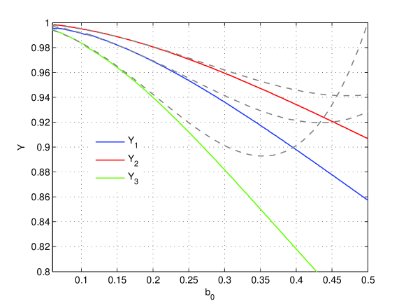
Figure 1: An exact and an approximate $Y$-functions comparison.

To obtain dispersion relations we use the eikonal approximation and represent the wave field in form: ${\bf e}_{w}={\bf e}\exp{\{iS({\bf r},t)\}},$ ${\bf b}_{w}={\bf b}\exp{\{iS({\bf r},t)\}},$ where ${\bf e}$ and ${\bf b}$ are the amplitudes and $S$ is the eikonal. As usual for the eikonal approximation, we will suppose that amplitude variations along the wave propagation ray are small and can be neglected in calculations. Substitution of ${\bf e}_{w}$, ${\bf b}_{w}$ and constitutive relations (10) to the ordinary equations of continuous media electrodynamics leads to homogeneous equations on wave field components:

$$\Pi_{\alpha\beta}{e}_{w}^{\beta}=0,$$ (16)

where indexes enumerate the cartesian components of the electric field vector $\alpha,\beta=1\ldots 3$ and $\Pi_{\alpha\beta}$ is the polarization tensor:

$$\Pi_{\alpha\beta}=\Big{\{}\Big{(}({\bf\nabla}S)^{2}-({\partial_{0}S})^{2}\Big{)}\delta_{\alpha\beta}-{\partial_{\alpha}S}{\partial_{\beta}S}\Big{\}}\times\Big{\{}1-2\zeta_{1}b_{0}^{2}\Big{\}}$$ (17)

$$-4\zeta_{3}\Big{[}{\bf\nabla}S{\bf b}_{0}\Big{]}_{\alpha}\Big{[}{\bf\nabla}S{\bf b}_{0}\Big{]}_{\beta}-4\zeta_{2}({\partial_{0}S})^{2}({\bf b}_{0})_{\alpha}({\bf b}_{0})_{\beta},$$

in which the following notations were used: $\partial_{0}=\partial/\partial(ct)$ and $\partial_{\alpha}$ denotes spatial coordinate $x^{\alpha}$ derivative, $\delta_{\alpha\beta}$ – is the Kronecker symbol, $\nabla$ – is the gradient operator, ${\bf b}_{0}={\bf B}_{0}/B_{c}$ and the square brackets refer to the vector cross-product. In should be noted that our result for polarization tensor is close to the similar one obtained in new1 . The existence of nontrivial solutions of (16) requires $\mbox{det}\|\Pi_{\alpha\beta}\|=0$ which finally leads to dispersion relations for the electromagnetic wave at the eikonal approximation:

$$\Big{\{}({\bf\nabla}S)^{2}-({\partial_{0}S})^{2}+4\zeta_{3}\Big{[}({\bf b}_{0}{\bf\nabla}S)^{2} - {b}_{0}^{2}({\bf\nabla}S)^{2}\Big{]}+2\zeta_{1}{b}_{0}^{2}\Big{[}({\partial_{0}S})^{2}-({\bf\nabla}S)^{2}\Big{]}\Big{\}}$$

$$\times\Big{\{}({\bf\nabla}S)^{2}-({\partial_{0}S})^{2}+4\zeta_{2}\Big{[}({\bf b}_{0}{\bf\nabla}S)^{2} - {b}_{0}^{2}({\partial_{0}S})^{2}\Big{]}+2\zeta_{1}{b}_{0}^{2}\Big{[}({\partial_{0}S})^{2}-({\bf\nabla}S)^{2}\Big{]}\Big{\}}$$ (18)

$$\times \Big{\{}2\zeta_{1}{b}_{0}^{2}-1\Big{\}}=0.$$

Multiplicative structure of obtained dispersion relations points to vacuum birefringence retention even in case of one-loop nonperturbative QED. The first factor in (3) corresponds to the dispersion law for a normal wave polarized perpendicular to external magnetic field ($\bot$-mode), whereas the second multiplier describes the mode polarized along the field ${\bf B}_{0}$ ($||$-mode). The last factor in (3) does not depend on the wave parameters and its equality to zero is expected at huge magnetic field intensities $B_{0}\sim B_{c}\exp{(1/\alpha)}$. Just for these values QED vacuum instability induced by magnetic field was predicted a25 . To avoid such a regime in future, we will consider field intensities much closer to $B_{c}$.

Now let us investigate the properties of normal waves in more detail, and use the obtained dispersion relations in strengthening some expectations for vacuum birefringence detection in experiment.

4 QED vacuum birefringence extension on nonperturbative regime

There are two traditional approaches to the interpretation of the dispersion relations for vacuum nonlinear electrodynamics. The first one comes from the representation of the vacuum as a continuous media. The vacuum birefringence in this case is explained by the normal modes refraction indexes mismatch $n_{\bot}\neq n_{||}$. The second approach assumes that the electromagnetic wave propagates in the space-time with the effective geometry following from the dispersion relations. This interpretation explains the vacuum birefringence due to the difference between the effective space-time metric tensors $G^{ik}_{\bot}\neq G^{ik}_{||}$ for each normal mode. For completeness, we use each of these approaches in the analysis of obtained dispersion relations.

For description in terms of refractive indexes one should substitute eikonal $S(t,{\bf r})=\omega t-({\bf k}{\bf r})$ to dispersion relations (3), and take into account the relation between the wave vector ${\bf k}$ and frequency $\omega$ which is ordinary for homogeneous wave in continuous media: ${\bf k}=\omega n{\bf q}/c$, where $n$ is the refraction index and ${\bf q}$ is the unity vector in wave propagation direction. Such substitution gives explicit expressions for the normal modes refraction indexes:

$$n_{\bot}^{2}=1+{4\zeta_{3}b_{0}^{2}\sin^{2}{\theta}\over 1-2b_{0}^{2}[\zeta_{1}+2\zeta_{3}\sin^{2}{\theta}]},\qquad n_{||}^{2}=1+{4\zeta_{2}b_{0}^{2}\sin^{2}{\theta}\over 1-2b_{0}^{2}[\zeta_{1}-2\zeta_{2}\cos^{2}{\theta}]},$$ (19)

where $\theta$ is an angle between the wave vector ${\bf k}$ and the magnetic field ${\bf B}_{0}$. These expression refine the results obtained earlier a26 in which the dependance on angle $\theta$ is more simple and the terms in denominator are neglected:

$$n_{\bot}^{2}\approx 1+{4\zeta_{3}b_{0}^{2}\sin^{2}{\theta}},\qquad n_{||}^{2}\approx 1+{4\zeta_{2}b_{0}^{2}\sin^{2}{\theta}},$$ (20)

which are close to results of a16 ; a26 obtained on the basis of a purely quantum approach with fixed selection of the gauge. As the angle dependance in the exact expressions (19) is different, it becomes possible to figure out are there any conditions under which $n_{\bot}=n_{||}$ and the birefringence is suppressed. The equality of the refractive indexes leads to the relation which is valid for any angle $\theta$:

$$(\zeta_{3}-\zeta_{2})(1-2\zeta_{1}b_{0}^{2})+4\zeta_{3}\zeta_{2}b_{0}^{2}=0.$$ (21)

However, the numerical calculations show that there are no solutions for this equation at any arbitrary magnetic field close to $B_{c}$ so the vacuum birefringence remains.

To analyze the dependence of refractive indexes on the magnetic field value, we will choose $\theta=\pi/2$, which is more valuable for experimental research because in this case indexes are maximal. As it follows from numerical calculations, the refractive index $n_{||}$ increases almost linearly in $1<b_{0}<100$ and shows nonlinear growth in wider field ranges. Whereas the $n_{\bot}$ tends to saturation at the value $(n_{\bot})_{sat}-1\approx 4\cdot 10^{-4}$ and ceases to depend on the field strength. The dependance of $n_{\bot,||}-1$ for $b_{0}<3$ is represented on the left graph in Figure 2. The right graph shows the exact difference $n_{||}-n_{\bot}$ coming from (19) and the same difference following from the perturbative QED: $n_{||}-n_{\bot}\approx 2(\eta_{2}-\eta_{1})b_{0}^{2}$, which is marked on the graph with a gray line. Despite the proximity of perturbative description, there is a good accordance to the exact result up to the field values $b_{0}\approx 2$. This indicates that more then order discrepancy between perturbative QED birefringence prediction and the experimental result obtained in PVLAS a8 is not associated with the inaccuracy of perturbative description and should have a more profound physical reason.

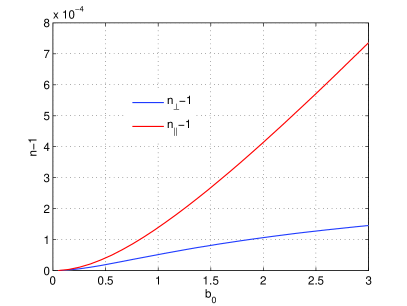
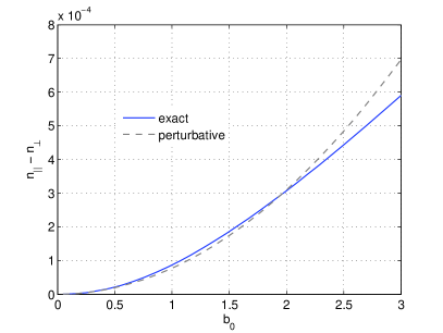
Figure 2: The refractive indexes and their difference depending on the magnetic field value $b_{0}=B_{0}/B_{c}$.

Another traditional approach to the dispersion relations interpretation is based on effective geometry representation. It assumes that the wave propagates in curved space-time, which geometry depends on external magnetic field. The dispersion relations (3), now are interpreted as Hamilton-Jacobi equation for a massless particle in the effective space-time with the metric tensor $G^{ik}_{\bot,||}$ correspondent to each normal mode:

$$\Big{[}G^{ik}_{\bot}{\partial S\over\partial x^{i}}{\partial S\over\partial x^{k}}\Big{]}\times\Big{[}G^{mn}_{||}{\partial S\over\partial x^{m}}{\partial S\over\partial x^{n}}\Big{]}=0.$$ (22)

As it follows from (3), the components of the effective metric tensor take the form:

$$G^{00}_{\bot} = g^{00},\quad G^{\alpha\beta}_{\bot}=g^{\alpha\beta}+{4\zeta_{3}\over 1-2\zeta_{1}b_{0}^{2}}\times(b_{0}^{2}\delta^{\alpha\beta}-b_{0}^{\alpha}b_{0}^{\beta}),$$ (23)

$$G^{00}_{||} = g^{00},\quad G^{\alpha\beta}_{||}=g^{\alpha\beta}+{4\zeta_{2}\over 1-2\zeta_{1}b_{0}^{2}+4\zeta_{2}b_{0}^{2}}\times(b_{0}^{2}\delta^{\alpha\beta}-b_{0}^{\alpha}b_{0}^{\beta}),$$ (24)

where $g^{ik}$ is Minkowski space-time metric tensor and the Greek indexes enumerate the spatial coordinates, so $\alpha,\beta=1..3$. It is easy to verify that in low-field limit $b_{0}\ll 1$ the expressions (23) take the form of perturbative QED effective metric tensor obtained in a11 :

$$G^{ik}_{\bot,||}\approx g^{ik}+4\eta_{1,2}(b_{0}^{2}\delta^{\alpha\beta}-b_{0}^{\alpha}b_{0}^{\beta}).$$ (25)

Such correspondence allows us to extend some predictions for vacuum birefringence manifestations obtained on base of perturbative metric tensor (25) to non-perturbative region by simple replacement of parameters:

$$\eta_{1}\to{\zeta_{3}\over 1-2\zeta_{1}b_{0}^{2}},\quad\eta_{2}\to{\zeta_{2}\over 1-2\zeta_{1}b_{0}^{2}+4\zeta_{2}b_{0}^{2}}.$$ (26)

For instance, such extension is especially actual for the pulsars and magnetars which are one the most attractive objects for QED regime tests. The magnetic fields of such astrophysical sources can significantly exceed critical limit $b_{0}=B_{0}/B_{c}\gg 1$. One of observable manifestations of the vacuum birefringence in pulsar neighbourhood is related to normal mode delay for hard X-ray and gamma- radiation pulses passing near the pulsar. Because of the vacuum birefringence, the propagation velocity of ${\bot}$-mode is greater then ${||}$-mode, so it will reach to the detector earlier. So the leading part of the pulse coming from the X-ray source to the detector will be linearly polarized due to the ${\bot}$-mode. This part of the pulse will have a time duration $\Delta t$. After this time the ${||}$-mode will reach the detector and the pulse polarization state will change to elliptical. The maximal estimation for the delay $\Delta t$ in perturbative QED was obtained in a11 :

$$\Delta t={123\pi(\eta_{2}-\eta_{1})b_{0}^{2}R_{s}\over 128c},$$ (27)

where $R_{s}$ is the pulsar radius, and $c$ is the speed of light in Maxwell vacuum. Birefringence expansion (26) allows us to estimate the order of magnitude for the time delay $\Delta t$ in nonperturbative regime:

$$\Delta t\simeq{b_{0}^{2}R_{s}\over c}\Big{[}{\zeta_{3}\over 1-2\zeta_{1}b_{0}^{2}}-{\zeta_{2}\over 1-2\zeta_{1}b_{0}^{2}+4\zeta_{2}b_{0}^{2}}\Big{]}.$$ (28)

The dependence of the time delay on magnetic field strength and its estimates for some pulsars and magnetars are represented on Figure 3. For the estimates we use the pulsar data from McGill a27 and ATNF a28 catalogs and also suppose the pulsar radius equal to $R_{s}=10km$.

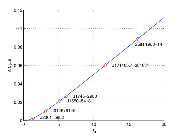
Figure 3: Time delay between ${\bot}$ and ${||}$-modes arrival to detector.

The delay value varies in hundredth of microseconds and this is sufficient for contemporary timing measurements. Furthermore the estimate can be enforced for the unique object J1808-2024 with the field strength $B_{0}\sim 2.06\cdot 10^{15}G$ for which the delay can reach $\Delta t\sim 0.3\mu s$. Also it should be noted that there is almost linear dependence between delay and field strength, instead of quadratic, typical for delay in perturbative regime (27), therefore the direct interpolation of perturbative description on the region $b_{0}>1$ will lead to overestimation for the delay.

5 Conclusion

In this paper we have investigated expansion of vacuum birefringence on nonperturbative regime of QED. The obtained constitutive relations (10) for weak electromagnetic wave propagating on background of a strong magnetic field indicate that this expansion consists of replacing of perturbative constants $\eta_{1},\eta_{2}$ by three functions $\zeta_{1},\zeta_{2},\zeta_{3}$, which depend on the external field strength. For vacuum birefringence description we have used a semiclassical approach in terms of the wave field strength which gives gauge independent results unlike most of the other calculations performed in the fixed gauge selection. In such approach the polarization tensor (17) and dispersion relations (3) were obtained and both interpreted in terms of refractive indexes and the effective space-time geometry. The refractive indexes interpretation confirmed the results obtained earlier by other authors on the base of quantum field theory methods. The comparison between the perturbative and nonperturbative refractive indexes, as expected, reveals an insignificant difference at weak field values $b_{0}\ll 1$, and this indicates that inaccuracy in QED theoretical description can not be a cause of discrepancy detected in the PVLAS experiment a9 . Another feature observed in the refractive indexes analysis is the possible saturation of $n_{||}$ at the strong external field values $b_{0}\gg 1$. Unfortunately, this feature can not be verified in conditions of the terrestrial facilities, however the astrophysical sources such as pulsars and magnetars provide a wider opportunities in QED features investigations. It is more convenient to use an effective geometry formalism for vacuum birefringence description in the neighbourhood of such field sources. The dispersion relations interpretation in terms of the effective geometry (23) allowed us to extend the predictions for the normal mode relative delay in the hard radiation propagating near the pulsar. The estimates for such delay for a different pulsars, show its detectability with contemporary experimental technique. Moreover, it was found out that the dependence between the delay and the field value predicted by nonperturbative QED is close to linear (Figure 3) and can be roughly expressed as $\Delta t=(5.8b_{0}-7)\times 10^{-3}\mu{s}$ for $2<b_{0}<100$. This dependence differs from the quadratic one following from the direct perturbative QED prediction extrapolation to the strong field region. As the perturbative QED is not valid for such field values, it gives overestimated result for delay. This feature can be noted in planning of future astrophysical missions aimed at the QED effects investigation in the pulsar fields, such as XIPE a30 .

References

- (1) W.Heisenberg and H.Euler, Consequences of Dirac’s Theory of Positrons, Z. Phys., 26, (1936) 714.
- (2) D.Hanneke and S.Fogwell and G.Gabrielse, New Measurement of the Electron Magnetic Moment and the Fine Structure Constant, Phys. Rev. Lett., 100, (2008) 120801.
- (3) M.Hayakawa, T.Kinoshita and M.Nio, Revised value of the eighth-order QED contribution to the anomalous magnetic moment of the electron, Phys. Rev. D, 77, (2008) 053012.
- (4) Sh.Zh.Akhmadaliev et al. Delbruck scattering at energies of 140-450 MeV, Phys.Rev. C, 58, (1998) 2844.
- (5) W.E.Lamb and R.C.Retherford Fine Structure of the Hydrogen Atom by a Microwave Method, Phys. Rev., 72, (1947) 241.
- (6) S.L.Adler, Photon splitting and photon dispersion in a strong magnetic field, Ann. Phys., 67, (1971) 599.
- (7) Sh.Zh.Akhmadaliev et al., Experimental Investigation of High-Energy Photon Splitting in Atomic Fields, Phys. Rev. Lett., 89, (2002) 061802.
- (8) F.Della Valle et al, The PVLAS experiment: measuring vacuum magnetic birefringence and dichroism with a birefringent Fabry-Perot, Eur. Phys. J. C, 76, (2016) 24.
- (9) F.Della Valle et al., First results from the new PVLAS apparatus : a new limit on vacuum magnetic birefringence, Phys Rev. D, 90, (2014) 092003.
- (10) S.Villalba-Ch’avez and A.Di Piazza, Axion-induced birefringence effects in laser driven nonlinear vacuum interaction, Journal of High Energy Physics, 11, (2013) 136.
- (11) V.I.Denisov and S.I.Svertilov, Nonlinear electromagnetic and gravitational actions of neutron star fields on electromagnetic wave propagation, Phys. Rev. D, 71, (2005) 063002.
- (12) J.Schwinger, On Gauge Invariance and Vacuum Polarization, Phys. Rev., 82, (1951) 664.
- (13) Sh.Zh.G.V. Dunne, New strong-field QED effects at extreme light infrastructure, Eur. Phys. J. D, 55, (2009) 327.
- (14) S.Bulanov et al., On the Schwinger limit attainability with extreme power lasers, Phys. Rev. Lett., 105, (2010) 220407.
- (15) K.Hattori and K.Itakura, Vacuum birefringence in strong magnetic fields: (I) Photon polarization tensor with all the Landau levels, Ann. of Phys., 330, (2013) 23.
- (16) K.Hattori and K.Itakura, Vacuum birefringence in strong magnetic fields: (II) Complex refractive index from the lowest Landau level, Ann. of Phys., 334, (2013) 58.
- (17) V.B.Berestetski, E.M.Lifshits, and L.P.Pitaevsky, Quantum Electrodynamics, Pergamon, Oxford (1982).
- (18) G.V.Dunne, Heisenberg-Euler Effective Lagrangians: Basics and Extensions, arxiv:hep-th/0406216v1.
- (19) W.Dittrich and H.Gies, Probing the quantum vacuum. Perturbative effective action approach in quantum electrodynamics and its application, Tracts Mod. Phys., 166, (2000).
- (20) V.Denisov, V.Sokolov, and M.Vasili’ev, Nonlinear vacuum electrodynamics birefringence effect in a pulsar’s strong magnetic field, Phys. Rev. D, 90, (2014) 023011.
- (21) R.Battesti and C.Rizzo, Magnetic and electric properties of a quantum vacuum Rept.Prog.Phys., 76, (2013) 016401.
- (22) V.Denisov, Nonlinear effect of quantum electrodynamics for experiments with a ring laser, J. Opt. A: Pure Appl. Opt., 2, (2000) 372.
- (23) J.Y.Kimand T.Lee, Nonlinear electrodynamic effect of light bending by charged astronomical objects, Nuovo Cimento. C, 1 suppl.1, (1976) 69.
- (24) V.Denisov and S.Svertilov, Vacuum nonlinear electrodynamics curvature of photon trajectories in pulsars and magnetars, A&A, 399, (2003) 39.
- (25) J.Schinger, Wu-YangTsai and T.Erber, Classical and quantum theory of synergic Syncrotron-Čherenkov radiation, Ann. Phys., 90 , (1976) 303.
- (26) T.Erber, D.White and Wu-YangTsai, Experimental aspects of Syncrotron-Čherenkov radiation, Ann. Phys., 102, (1976) 405.
- (27) F.Karbstein and R.Shaisultanov, Photon propagation in slowly varying inhomogeneous electromagnetic fields, Phys. Rev. D, 91, (2015) 085027.
- (28) A.E.Shabad and V.V.Usov, Effective Lagrangian in nonlinear electrodynamics and its properties of causality and unitarity, Phys. Rev. D, 83, (2011) 105006
- (29) T.Erber and Wu-YangTsai, Propogation of photon in homogeneous magnetic fields: Index of refraction, Phys. Rev. D , 12, (1975) 1132.
- (30) S.A.Olausen and V.M. Kaspi, The McGill magnetar catalog, The Astrophysical Journal Supplement Series, 212, (2014) 1.
- (31) http://www.atnf.csiro.au/research/pulsar/psrcat/
- (32) P.Soffitta, XIPE: the X-ray imaging polarimetry explorer, Experimental Astronomy, 36, (2013) 523.