Efficient Inexact Proximal Gradient Algorithm for Nonconvex Problems

Abstract

The proximal gradient algorithm has been popularly used for convex optimization. Recently, it has also been extended for nonconvex problems, and the current state-of-the-art is the nonmonotone accelerated proximal gradient algorithm. However, it typically requires two exact proximal steps in each iteration, and can be inefficient when the proximal step is expensive. In this paper, we propose an efficient proximal gradient algorithm that requires only one inexact (and thus less expensive) proximal step in each iteration. Convergence to a critical point is still guaranteed and has a $O(1/k)$ convergence rate, which is the best rate for nonconvex problems with first-order methods. Experiments on a number of problems demonstrate that the proposed algorithm has comparable performance as the state-of-the-art, but is much faster.

1 Introduction

In regularized risk minimization, we consider optimization problems of the form

$$\min_{x}F(x)\equiv f(x)+g(x),$$ (1)

where $f$ is the loss, and $g$ is the regularizer. Typically, $f$ is smooth and convex (e.g., square and logistic losses), and $g$ is convex but may not be differentiable (e.g., $\ell_{1}$ and nuclear norm regularizers). The proximal gradient (PG) algorithm Parikh and Boyd (2014), together with its accelerated variant (APG) Beck and Teboulle (2009b); Nesterov (2013), have been popularly used for solving this convex problem. Its crux is the proximal step $\text{prox}_{g}(\cdot)=\arg\min_{x}\frac{1}{2}\|x-\cdot\|_{2}^{2}+\eta g(x)$, which can often be easily computed in closed-form.

While convex regularizers are easy to use, the resultant predictors may be biased Zhang (2010). Recently, there is growing interest in the use of nonconvex regularizers, such as the log-sum-penalty Candès et al. (2008) and capped $\ell_{1}$-norm Zhang (2010) regularizers. It has been shown that these often lead to sparser and more accurate models Gong et al. (2013); Lu et al. (2014); Zhong and Kwok (2014); Yao et al. (2015). However, the associated proximal steps become more difficult to compute analytically, and cheap closed-form solutions exist only for some simple nonconvex regularizers Gong et al. (2013). This is further aggravated by the fact that the state-of-the-art PG algorithm for nonconvex optimization, namely the nonmonotone accelerated proximal gradient (nmAPG) algorithm Li and Lin (2015), needs more than one proximal steps in each iteration.

When the optimization objective is convex, one can reduce the computational complexity of the proximal step by only computing it inexactly (i.e., approximately). Significant speedup has been observed in practice, and the resultant inexact PG algorithm has the same convergence guarantee as the exact algorithm under mild conditions Schmidt et al. (2011). However, on nonconvex problems, the use of inexact proximal steps has not been explored. Moreover, convergence of nmAPG hinges on the use of exact proximal steps.

In this paper, we propose a new PG algorithm for nonconvex problems. Unlike nmAPG, it performs only one proximal step in each iteration. Moreover, the proximal step can be inexact. The algorithm is guaranteed to converge to a critical point of the nonconvex objective. Experimental results on nonconvex total variation models and nonconvex low-rank matrix learning show that the proposed algorithm is much faster than nmAPG and other state-of-the-art, while still producing solutions of comparable quality.

The rest of the paper is organized as follows. Section 2 provides a brief review on the PG algorithm and its accelerated variant. The proposed algorithm is described in Section 3, and its convergence analysis studied in Section 4. Experimental results are presented in Section 5, and the last section gives some concluding remarks.

2 Related Work

In this paper, we assume that $f$ in (1) is $L$-Lipschitz smooth (i.e., $\|\nabla f(x)-\nabla f(y)\|_{2}\leq L\|x-y\|_{2}$), and $g$ is proper, lower semi-continuous. Besides, $F=f+g$ in (1) is bounded from below, and $\lim_{\|x\|_{2}\rightarrow\infty}F(x)=\infty$. Moreover, both $f$ and $g$ can be nonconvex.

First, we consider the case where $f$ and $g$ in (1) are convex. At iteration $k$, the accelerated proximal gradient (APG) algorithm generates $x_{k+1}$ as

$$y_{k} = x_{k}+\theta_{k}(x_{k}-x_{k-1}),$$ (2)

$$x_{k+1} = \text{prox}_{\eta g}(y_{k}-\eta\nabla f(y_{k})),$$ (3)

where $\theta_{k}=\frac{k-1}{k+2}$ and $\eta$ is the stepsize Beck and Teboulle (2009b); Nesterov (2013). When $\theta_{k}=0$, APG reduces to the plain PG algorithm.

On nonconvex problems, $y_{k}$ can be a bad extrapolation and the iterations in (2), (3) may not converge Beck and Teboulle (2009a). Recently, a number of PG extensions have been proposed to alleviate this problem. The iPiano Ochs et al. (2014), NIPS Ghadimi and Lan (2015), and UAG Ghadimi and Lan (2015) algorithms allow $f$ to be nonconvex, but still requires $g$ to be convex. The GD algorithm Attouch et al. (2013) also allows $g$ to be nonconvex, but does not support acceleration.

The current state-of-the-art is the nonmonotone APG (nmAPG) algorithm Li and Lin (2015), shown in Algorithm 1. It allows both $f$ and $g$ to be nonconvex, and also uses acceleration. To guarantee convergence, nmAPG ensures that the objective is sufficiently reduced in each iteration:

$$F(x_{k+1})\leq F(x_{k})-\frac{\delta}{2}\|v_{k+1}-x_{k}\|_{2}^{2},$$ (4)

where $v_{k+1}=\text{prox}_{\eta g}(x_{k}-\eta\nabla f(x_{k}))$ and $\delta>0$ is a constant. A second proximal step has to be performed (step 8) if a variant of (4) is not met (step 5).

Algorithm 1 Nonmonotone APG (nmAPG).

0:  choose $\eta\in(0,1/L)$, a positive constant $\delta$, $\Delta_{1}=F(x_{1})$, $q_{1}=1$, and $\nu\in(0,1)$;

1:  $x_{0}=x_{1}=x^{a}_{1}=0$ and $t_{0}=t_{1}=1$;

2:  for $k=1,\dots,K$ do

3:     $y_{k}=x_{k}+\frac{t_{k-1}}{t_{k}}(x^{a}_{k}-x_{k-1})+\frac{t_{k-1}-1}{t_{k}}(x_{k}-x_{k-1})$;

4:     $x^{a}_{k+1}=\text{prox}_{\eta g}(y_{k}-\eta\nabla f(y_{k}))$;

5:     if $F(x^{a}_{k+1})\leq\Delta_{k}-\frac{\delta}{2}\|x^{a}_{k+1}-y_{k}\|_{2}^{2}$ then

6:        $x_{k+1}=x^{a}_{k+1}$;

7:     else

8:        $x^{p}_{k+1}=\text{prox}_{\eta g}(x_{k}-\eta\nabla f(x_{k}))$;

9:        $x_{k+1}=\begin{cases}x^{a}_{k+1}&F(x^{a}_{k+1})\leq F(x^{p}_{k+1})\\ x^{p}_{k+1}&\text{otherwise}\end{cases}$;

10:     end if

11:     $q_{k+1}=\nu q_{k}+1$;

12:     $t_{k+1}=\frac{1}{2}\left((4t_{k}^{2}+1)^{1/2}+1\right)$;

13:     $\Delta_{k+1}=\frac{1}{q_{k+1}}(\nu q_{k}\Delta_{k}+F(x_{k+1}))$;

14:  end for

15:  return  $x_{K+1}$.

3 Efficient APG for Nonconvex Problems

The proposed algorithm is shown in Algorithm 2. Following Schmidt et al. (2011), we use a simpler acceleration scheme in step 3. Efficiency of the algorithm comes from two key ideas: reducing the number of proximal steps to one in each iteration (Section 3.1); and the use of inexact proximal steps (Section 3.2). Besides, we also allow nonmonotone update on the objective (and so $F(y_{k})$ may be larger than $F(x_{k})$). This helps to jump from narrow curved valley and improve convergence Grippo and Sciandrone (2002); Wright et al. (2009); Gong et al. (2013). Note that when the proximal step is inexact, nmAPG does not guarantee convergence as its Lemma 2 no longer holds.

Algorithm 2 Noconvex inexact APG (niAPG) algorithm.

0:  choose $\eta\in(0,\frac{1}{L})$ and $\delta\in(0,\frac{1}{\eta}-L)$;

1:  $x_{0}=x_{1}=0$;

2:  for $k=1,\dots,K$ do

3:     $y_{k}=x_{k}+\frac{k-1}{k+2}(x_{k}-x_{k-1})$;

4:     $\Delta_{k}=\max_{t=\max(1,k-q),\dots,k}F(x_{t})$;

5:     if $F(y_{k})\leq\Delta_{k}$ then

6:        $v_{k}=y_{k}$;

7:     else

8:        $v_{k}=x_{k}$;

9:     end if

10:     $z_{k}=v_{k}-\eta\nabla f(v_{k})$;

11:     $x_{k+1}=\text{prox}_{\eta g}(z_{k})$; // possibly inexact

12:  end for

13:  return  $x_{K+1}$.

3.1 Using Only One Proximal Step

Recall that on extending APG to nonconvex problems, the key is to ensure a sufficient decrease of the objective in each iteration. Let $\rho=1/\eta$. For the standard PG algorithm with exact proximal steps, the decrease in $F$ can be bounded as follows.

Proposition 3.1 (Gong et al. (2013); Attouch et al. (2013)).

$F(x_{k+1})\leq F(x_{k})-\frac{\rho-L}{2}\|x_{k+1}-x_{k}\|_{2}^{2}$.

In nmAPG (Algorithm 1), there is always a sufficient decrease after performing the (non-accelerated) proximal descent from $x_{k}$ to $x^{p}_{k+1}$ (Proposition 3.1), but not necessarily the case for the accelerated descent from $x_{k}$ to $x^{a}_{k+1}$ (which is generated by a possibly bad extrapolation $y_{k}$). Hence, nmAPG needs to perform extra checking at step 5. If the condition fails, $x^{p}_{k+1}$ is used instead of $x^{a}_{k+1}$ in step 9.

As the main problem is on $y_{k}$, we propose to check $F(y_{k})$ (step 5 in Algorithm 2) before the proximal step (step 11), instead of checking after the proximal steps. Though this change is simple, the main difficulty is how to guarantee convergence while simultaneously maintaining acceleration and using only one proximal step. As will be seen in Section 4.1, existing proofs do not hold even with exact proximal steps.

The following shows that a similar sufficient decrease condition can still be guaranteed after this modification.

Proposition 3.2.

With exact proximal steps in Algorithm 2, $F(x_{k+1})\leq\min\left(F(y_{k}),\Delta_{k}\right)-\frac{\rho-L}{2}\|x_{k+1}-v_{k}\|_{2}^{2}$.

In step 4, setting $q=0$ is the most straightforward. The $F(y_{k})$ value is then checked w.r.t. the most recent $F(x_{k})$. The use of a larger $q$ is inspired from the Barzilai-Borwein scheme for unconstrained smooth minimization Grippo and Sciandrone (2002). This allows $y_{k}$ to occasionally increase the objective, while ensuring $F(y_{k})$ to be smaller than the largest objective value from the last $q$ iterations. In the experiments, $q$ is set to $5$ as in Wright et al. (2009); Gong et al. (2013).

3.2 Inexact Proximal Step

Proposition 3.2 requires exact proximal step, which can be expensive. Inexact proximal steps are much cheaper, but the inexactness has to be carefully controlled to ensure convergence. We will propose two such schemes depending on whether $g$ is convex. Note that $f$ is not required to be convex.

Convex $g$. As $g$ is convex, the optimization problem associated with the proximal step is also convex. Let $h_{\eta g}(x)\equiv\frac{1}{2}\|x-z_{k}\|_{2}^{2}+\eta g(x)$ be the objective in the proximal step. For any $z_{k}$, the dual of the proximal step at $z_{k}$ can be obtained as

$$\max_{w}\mathcal{D}_{\eta g}(w)\equiv\eta\left(z_{k}^{\top}w-g^{*}(w)\right)-\frac{\eta^{2}}{2}\|w\|_{2}^{2},$$ (5)

where $g^{*}$ is the convex conjugate of $g$. In an inexact proximal step, the obtained dual variable $\tilde{w}_{k}$ only approximately maximizes (5). The duality gap $\varepsilon_{k}\equiv h_{\eta g}(x_{k+1})-\mathcal{D}_{\eta g}(\tilde{w}_{k})$, where $x_{k+1}=z_{k}-\eta\tilde{w}_{k}$, upper-bounds the approximation error of the inexact proximal step $\epsilon_{k}\equiv h_{\eta g}(x_{k+1})-h_{\eta g}\left(\text{prox}_{\eta g}(z_{k})\right)$. To ensure the inexactness $\epsilon_{k}$ to be smaller than a given threshold $\tau_{k}$, we can control the duality gap as $\varepsilon_{k}\leq\tau_{k}$ Schmidt et al. (2011).

The following shows that $x_{k+1}$ satisfies a similar sufficient decrease condition as in Proposition 3.2. Note that this cannot be derived from Schmidt et al. (2011), which relies on the convexity of $f$.

Proposition 3.3.

$\!\!F(x_{k+1})\!\leq\!F(v_{k})-\frac{\rho-L}{2}\|x_{k+1}\!-\!v_{k}\|_{2}^{2}+\rho\varepsilon_{k}$.

Nonconvex $g$. When $g$ is nonconvex, the GD algorithm Attouch et al. (2013) allows inexact proximal steps. However, it does not support acceleration, and nonmonotone update. Thus, its convergence proof cannot be used here.

As $g$ is nonconvex, it is difficult to derive the dual of the corresponding proximal step, and the optimal duality gap may also be nonzero. Thus, we monitor the progress of $F$ instead. Inspired by Proposition 3.1, we require $x_{k+1}$ from an inexact proximal step to satisfy the following weaker condition:

$$F(x_{k+1})\leq F(v_{k})-\frac{\delta}{2}\|x_{k+1}-v_{k}\|_{2}^{2},$$ (6)

where $\delta\in(0,\rho-L)$. This condition has also been used in the GD algorithm. However, it requires checking an extra condition which is impractical.

We could have also used condition (6) when $g$ is convex. However, Proposition 3.3 offers more precise control, as it can recover (6) by setting $\varepsilon_{k}=\frac{\rho-L-\delta}{2\rho}\|x_{k+1}-v_{k}\|_{2}^{2}$ (note that $\delta<\rho-L$). Besides, the duality gap $\varepsilon_{k}$ is readily produced by primal-dual algorithms, and is often less expensive to compute than $F$.

4 Convergence Analysis

Definition 4.1 (Attouch et al. (2013)).

The Frechet subdifferential of $F$ at $x$ is

$$\hat{\partial}F(x)=\left\{u:\lim_{y\neq x}\inf_{y\rightarrow x}\frac{F(y)-F(x)-u^{\top}(y-x)}{\|y-x\|_{2}}\geq 0\right\}.$$

The limiting subdifferential (or simply subdifferential) of $F$ at $x$ is $\partial F(x)=\{u:\exists x_{k}\rightarrow x,F(x_{k})\rightarrow F(x),u_{k}\in\hat{\partial}F(x_{k})\!\rightarrow\!u,\text{ as }k\rightarrow\infty\}$.

Definition 4.2 (Attouch et al. (2013)).

$x$ is a critical point of $F$ if $0\in\nabla f(x)+\partial g(x)$.

4.1 Exact Proximal Step

In this section, we will show that Algorithm 2 (where both $f$ and $g$ can be nonconvex) converges with a $O(1/K)$ rate. This is the best known rate for nonconvex problems with first-order methods Nesterov (2004). A similar $O(1/K)$ rate for $\|\mathcal{G}(v_{k})\|_{2}^{2}$ is recently established for APG with nonconvex $f$ but only convex $g$ Ghadimi and Lan (2015). Note also that no convergence rate has been proved for nmAPG Li and Lin (2015) and GD Attouch et al. (2013) in this case. Besides, their proof techniques cannot be used here as their nonmonotone updates are different.

Theorem 4.1.

The sequence $\{x_{k}\}$ generated from Algorithm 2 (with exact proximal step) have at least one limit point, and all limit points are critical points of (1).

Let $\mathcal{G}(v)=v-\text{prox}_{\eta g}(v-\eta\nabla f(v))$, the proximal mapping at $v$ Parikh and Boyd (2014). The following Lemma suggests that $\|\mathcal{G}(v)\|_{2}^{2}$ can be used to measure how far $v$ is from optimality Ghadimi and Lan (2015).

Lemma 4.2 (Gong et al. (2013); Attouch et al. (2013)).

$v$ is a critical point of (1) if and only if $\mathcal{G}(v)=0$.

The following Proposition shows that the proposed Algorithm 2 converges with a $O(1/K)$ rate.

Proposition 4.3.

Let $\phi(k)=\arg\min_{t=\max(k-q,1),\dots,k}$ $\|x_{t+1}-v_{t}\|_{2}^{2}$. (i) $\lim_{k\rightarrow\infty}\|\mathcal{G}(v_{\phi(k)})\|_{2}^{2}=0$; and (ii) $\min_{k=1,\dots,K}\|\mathcal{G}(v_{{\phi(k)}})\|_{2}^{2}\leq\frac{2(q+1)c_{1}}{(\rho-L)K}$, where $c_{1}=\max_{t=1,\dots,q+1}F(x_{t})-\inf F$.

Table 1: Results on the image inpainting experiment (CPU time is in seconds).

		$\lambda=0.01$		$\lambda=0.02$		$\lambda=0.04$
		RMSE	CPU time	RMSE	CPU time	RMSE	CPU time
(nonconvex)	GDPAN	0.0326$\pm$0.0001	212.1$\pm$50.9	0.0301$\pm$0.0001	172.6$\pm$28.4	0.0337$\pm$0.0001	151.6$\pm$57.0
	nmAPG	0.0323$\pm$0.0001	600.5$\pm$35.8	0.0299$\pm$0.0001	461.7$\pm$33.3	0.0335$\pm$0.0001	535.6$\pm$29.7
	niAPG(exact)	0.0323$\pm$0.0001	307.4$\pm$26.8	0.0299$\pm$0.0001	297.2$\pm$35.3	0.0335$\pm$0.0001	282.7$\pm$19.3
	niAPG	0.0323$\pm$0.0002	91.6$\pm$10.8	0.0299$\pm$0.0001	77.1$\pm$7.4	0.0335$\pm$0.0001	56.5$\pm$9.4
(convex)	ADMM	0.0377$\pm$0.0001	55.7$\pm$5.1	0.0337$\pm$0.0001	54.7$\pm$1.4	0.0362$\pm$0.0001	33.2$\pm$1.5

Table 2: Matrix completion performance on the synthetic data (CPU time in seconds). Here, NMSE is scaled by $\times 10^{-2}$. Group (I) is based on convex nuclear norm regularization; group (II) on factorization model; and group (III) on nonconvex model (8).

		$m=500$ (observed: $12.43\%$)			$m=1000$ (observed: $6.91\%$)			$m=2000$ (observed: $3.80\%$)
		NMSE	rank	CPU time	NMSE	rank	CPU time	NMSE	rank	CPU time
(I)	active	4.10$\pm$0.16	42	11.8$\pm$1.1	4.08$\pm$0.11	55	77.6$\pm$8.4	3.92$\pm$0.04	71	507.3$\pm$25.4
	ALT-Impute	3.99$\pm$0.15	42	1.9$\pm$0.2	3.87$\pm$0.09	55	29.4$\pm$1.2	3.68$\pm$0.03	71	143.1$\pm$3.9
(II)	AltGrad	2.99$\pm$0.45	5	0.2$\pm$0.1	2.73$\pm$0.21	5	0.4$\pm$0.1	2.67$\pm$0.27	5	1.2$\pm$0.2
	R1MP	23.04$\pm$1.27	45	0.3$\pm$0.1	21.39$\pm$0.94	54	0.9$\pm$0.1	20.11$\pm$0.28	71	2.7$\pm$0.2
(III)	IRNN	1.96$\pm$0.05	5	19.2$\pm$1.2	1.88$\pm$0.04	5	215.1$\pm$4.3	1.80$\pm$0.03	5	3009.5$\pm$35.9
	FaNCL	1.96$\pm$0.05	5	0.4$\pm$0.1	1.88$\pm$0.04	5	1.4$\pm$0.1	1.80$\pm$0.03	5	5.6$\pm$0.2
	nmAPG	1.96$\pm$0.05	5	2.3$\pm$0.2	1.88$\pm$0.03	5	6.9$\pm$0.3	1.80$\pm$0.03	5	27.1$\pm$4.0
	niAPG(exact)	1.96$\pm$0.04	5	1.8$\pm$0.2	1.88$\pm$0.03	5	5.3$\pm$0.5	1.80$\pm$0.04	5	18.4$\pm$2.2
	niAPG	1.96$\pm$0.05	5	0.1$\pm$0.1	1.88$\pm$0.03	5	0.4$\pm$0.1	1.80$\pm$0.04	5	1.2$\pm$0.2

4.2 Inexact Proximal Step

Convex $g$. As in Schmidt et al. (2011), we assume that the duality gap $\varepsilon_{k}$ decays as $O(1/k^{1+\varsigma})$ for some $\varsigma>0$. Let $c\equiv\sum_{k=1}^{\infty}\varepsilon_{k}$. Note that $c<\infty$.

Theorem 4.4.

The sequence $\{x_{k}\}$ generated from Algorithm 2 have at least one limit point, and all limit points are critical points of (1).

Proposition 4.5.

Let $e_{k}\equiv x_{k+1}-\text{prox}_{\eta g}(x_{k}-\eta\nabla f(x_{k}))$, the difference between the inexact and exact proximal step solutions at iteration $k$. We have $\|e_{k}\|_{2}^{2}\leq 2\varepsilon_{k}$.

Note that the proof techniques in Schmidt et al. (2011) cannot be used here as $f$ is not required to be convex. As in Proposition 4.3, we also use $\|\mathcal{G}(v_{\phi(k)})\|_{2}^{2}$ to measure how far $v_{\phi(k)}$ is from optimality.

Proposition 4.6.

(i) $\lim_{k\rightarrow\infty}\|\mathcal{G}(v_{\phi(k)})\|_{2}^{2}=0$; and (ii) $\min_{k=1,\dots,K}\|\mathcal{G}(v_{\phi(k)})\|_{2}^{2}\leq\frac{2}{K}(4c+\frac{(q+1)(c_{1}+\rho c)}{\rho-L})$.

When all $\varepsilon_{k}$’s are zero, Proposition 4.6 reduces to Proposition 4.3. In general, the bound of $\min_{k=1,\dots,K}\|\mathcal{G}(v_{\phi(k)})\|_{2}^{2}$ in Proposition 4.6 is larger due to the inexact proximal step.

Nonconvex $g$. With inexact proximal steps, nmAPG no longer guarantees convergence, and its proof cannot be easily extended. On the other hand, GD allows inexact proximal steps but uses a different approach to control inexactness. Moreover, it does not support acceleration.

The following shows that Algorithm 2 generates a bounded sequence, and Corollary 4.8 shows that the limit points are critical points.

Theorem 4.7.

The sequence $\{x_{k}\}$ generated from Algorithm 2 has at least one limit point.

Corollary 4.8.

Let $\{x_{k_{j}}\}$ be a subsequence of $\{x_{k}\}$ with $\lim_{k_{j}\rightarrow\infty}x_{k_{j}}=x_{*}$. If (i) $x_{k+1}\neq v_{k}$ unless $v_{k}=\text{prox}_{\eta g}(v_{k}-\eta\nabla f(v_{k}))$, and (ii) $\lim_{k_{j}\rightarrow\infty}F(x_{k_{j}})=F(x_{*})$, then $x_{*}$ is a critical point of (1).

Assumption (i), together with Lemma 4.2, ensures that the sufficient decrease condition in (6) will not be trivially satisfied by $x_{k+1}=v_{k}$, unless $v_{k}$ is a critical point. Assumption (ii) follows from Definition 4.1, as the subdifferential is defined by a limiting process.

Proposition 4.9.

Attouch et al. (2013) Assumption (ii) is satisfied when (i) the proximal step is exact; or (ii) $g$ is continuous or is the indicator function of a compact set.

When the proximal step is exact or when $g$ is convex, $\mathcal{G}(\cdot)$ has been used to measure the distance from optimality. However, this is inappropriate when $g$ is nonconvex and the proximal step is inexact, as the inexactness can no longer be directly controlled. Instead, we will measure optimality via $a_{k}\equiv\|x_{k+1}-v_{k}\|_{2}^{2}$.

Proposition 4.10.

(i) $\lim_{k\rightarrow\infty}a_{k}=0$; and (ii) $\min_{k=1,\dots,K}a_{\phi(k)}\leq\frac{2(q+1)c_{1}}{\delta K}$.

When the proximal step is exact, $x_{k+1}=\text{prox}_{\eta g}(v_{k}-\eta\nabla f(v_{k}))$, and $a_{k}=\|\mathcal{G}(v_{k})\|_{2}^{2}$. Proposition 4.10 then reduces to Proposition 4.3 (but with a looser bound).

Table 3: Results on the MovieLens data sets (CPU time in seconds). Here, RMSE is scaled by $10^{-1}$. Group (I) is based on convex nuclear norm regularization; group (II) on factorization model; and group (III) on nonconvex model (8).

		MovieLens-1M			MovieLens-10M			MovieLens-20M
		RMSE	rank	CPU time	RMSE	rank	CPU time	RMSE	rank	CPU time
(I)	active	8.20$\pm$0.01	68	50.5$\pm$1.6	8.14$\pm$0.01	101	1520.8$\pm$18.2	8.02$\pm$0.01	197	7841.9$\pm$666.3
	ALT-Impute	8.18$\pm$0.01	68	34.0$\pm$1.1	8.14$\pm$0.01	101	821.7$\pm$34.5	8.01$\pm$0.01	197	3393.2$\pm$220.3
(II)	AltGrad	8.02$\pm$0.03	6	4.0$\pm$1.1	7.97$\pm$0.04	9	94.5$\pm$30.8	7.94$\pm$0.04	10	298.3$\pm$54.1
	R1MP	8.53$\pm$0.02	13	1.3$\pm$0.2	8.52$\pm$0.04	23	58.8$\pm$11.0	8.54$\pm$0.02	26	139.2$\pm$23.7
(III)	FaNCL	7.88$\pm$0.01	5	12.5$\pm$0.9	7.79$\pm$0.01	8	703.5$\pm$18.3	7.84$\pm$0.03	9	2296.9$\pm$176.4
	nmAPG	7.87$\pm$0.01	5	12.5$\pm$0.9	7.80$\pm$0.01	8	627.5$\pm$16.4	7.85$\pm$0.01	9	1577.9$\pm$103.2
	niAPG(exact)	7.87$\pm$0.01	5	11.1$\pm$0.8	7.79$\pm$0.01	8	403.1$\pm$19.6	7.84$\pm$0.01	9	1111.9$\pm$65.3
	niAPG	7.87$\pm$0.01	5	2.7$\pm$0.3	7.79$\pm$0.01	8	90.2$\pm$2.6	7.85$\pm$0.01	9	257.6$\pm$33.4

Table 4: Number of proximal steps on the synthetic and recommender system data sets.

	Synthetic			MovieLens			Netflix	Yahoo
	$m=$500	$m=$1000	$m=$2000	1M	10M	20M
nmAPG	77	104	145	95	221	236	183	579
niAPG(exact)	64 ($\downarrow\!\!17\%$)	85 ($\downarrow\!\!18\%$)	115 ($\downarrow\!\!21\%$)	82 ($\downarrow\!\!13\%$)	143 ($\downarrow\!\!35\%$)	165 ($\downarrow\!\!31\%$)	133 ($\downarrow\!\!27\%$)	425 ($\downarrow\!\!26\%$)
niAPG	64 ($\downarrow\!\!17\%$)	85 ($\downarrow\!\!18\%$)	115 ($\downarrow\!\!21\%$)	81 ($\downarrow\!\!15\%$)	140 ($\downarrow\!\!36\%$)	160 ($\downarrow\!\!32\%$)	132 ($\downarrow\!\!28\%$)	413 ($\downarrow\!\!29\%$)

5 Experiments

In this section, we perform experiments when $g$ is convex (Section 5.1) and nonconvex (Section 5.2).

5.1 Image Inpainting

The total variation (TV) model Beck and Teboulle (2009a) has been popularly used in image processing. Let $y\in\mathbb{R}^{d}$ be the vectorized input image and $x\in\mathbb{R}^{d}$ be the recovered one. We consider the TV model with nonconvex log-sum-penalty regularizer Candès et al. (2008).

$$\min_{x}\frac{1}{2}\|M\odot(x-y)\|_{2}^{2}+\lambda\sum_{i=1}^{d}\kappa([D_{h}x]_{i})+\kappa([D_{v}x]_{i}),$$ (7)

where $M\in\{0,1\}^{d}$ is a mask such that $M_{ij}=1$ indicates that the corresponding pixel is observed, $D_{h}$ and $D_{v}$ are the horizontal and vertical partial derivative operators, $\odot$ is the elementwise multiplication, and $\kappa(\alpha)=\log(1+|\alpha|)$.

As suggested in Yao and Kwok (2016), (7) can be transformed as the minimization of $f(x)+\lambda\,\text{TV}(x)$, where $f(x)=\frac{1}{2}\|M\odot(x-y)\|_{2}^{2}-\lambda[\,\text{TV}(x)+\sum_{i=1}^{d}\kappa([D_{h}x]_{i})+\kappa([D_{v}x]_{i})]$ is nonconvex but smooth, and $\,\text{TV}(x)=\|D_{h}x\|_{1}+\|D_{v}x\|_{1}$ is the standard (convex) TV regularizer. Thus, we only need to handle the proximal step of the TV regularizer, which will be computed numerically by solving its dual using L-BFGS Beck and Teboulle (2009a).

The following solvers on the transformed problems are compared: (i) GDPAN Zhong and Kwok (2014), which performs gradient descent with the proximal average; (ii) nmAPG; (iii) the proposed niAPG, in which inexactness of the proximal step is controlled by decaying the duality gap $\varepsilon_{k}$ at a rate of $O(1/k^{1.5})$; and (iv) the exact version of niAPG(exact), which simulates an exact proximal step with a small duality gap (${10}^{-4}$). We do not compare with the GD algorithm Attouch et al. (2013), as its inexactness condition is difficult to check and it does not use acceleration.

As a further baseline, we compare with the convex TV model: $\min_{x}\frac{1}{2}\|M\odot(x-y)\|_{2}^{2}+\lambda(\|D_{v}x\|_{1}+\|D_{h}x\|_{1})$, which is solved using ADMM Boyd et al. (2011). We do not compare with CCCP Yuille and Rangarajan (2002), which is slow in practice Yao and Kwok (2016).

Experiments are performed on the “Lena” image. We normalize the pixel values to $[0,1]$, and then add Gaussian noise from $\mathcal{N}(0,0.05)$. $50\%$ of the pixels are randomly sampled as observed. For performance evaluation, we report the CPU time and root-mean-squared error (RMSE) on the whole image. The experiment is repeated five times. Results are shown in Table 1. Figure 1 plots convergence of the objective. As can be seen, the nonconvex TV model has better RMSE than the convex one. Among the nonconvex models, niAPG is much faster, as it only requires a small number of cheap inexact proximal steps (Table 5).

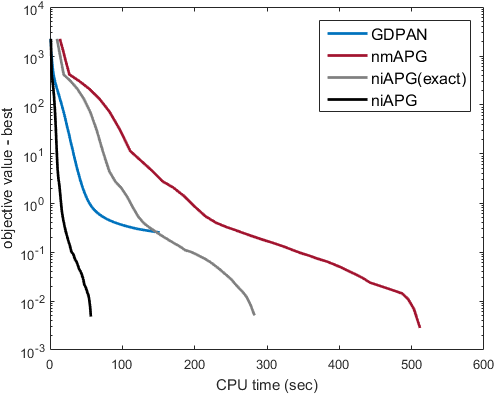
(a) $\lambda=0.02$.

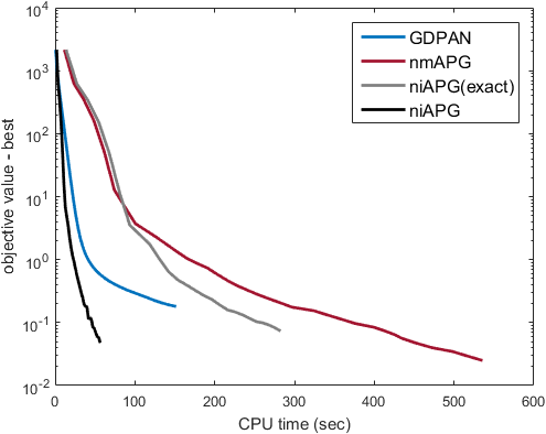
(b) $\lambda=0.04$.

Figure 1: Objective value vs CPU time on the image data.

Table 5: Number of proximal steps on image data. Number in brackets is the percentage reduction w.r.t. nmAPG.

	$\lambda=0.01$	$\lambda=0.02$	$\lambda=0.04$
nmAPG	87	46	43
niAPG(exact)	47 ($\downarrow\!\!46\%$)	35 ($\downarrow\!\!24\%$)	29 ($\downarrow\!\!33\%$)
niAPG	57 ($\downarrow\!\!35\%$)	41 ($\downarrow\!\!11\%$)	28 ($\downarrow\!\!35\%$)

(a) MovieLens-20M.

(b) Netflix.

(c) Yahoo.

Figure 2: Testing RMSE vs CPU time on the recommendation system data sets.

5.2 Matrix Completion

In this section, we consider matrix completion with a nonconvex low-rank regularizer. As shown in Lu et al. (2014); Yao et al. (2015), it gives better performance than nuclear-norm based and factorization approaches. The optimization problem can be formulated as

$$\min_{\text{rank}(X)\leq r}\frac{1}{2}\|P_{\Omega}(X_{ij}-O_{ij})\|_{F}^{2}+\lambda\sum_{i=1}^{r}\kappa\left(\sigma_{i}(X)\right),$$ (8)

where $O_{ij}$s are the observations, $\Omega_{ij}=1$ if $O_{i,j}$ is observed, and 0 otherwise, $\sigma_{i}(X)$ is the $i$th leading singular value of $X$, and $r$ is the desired rank. The associated proximal step can be solved with rank-$r$ SVD Lu et al. (2014).

Synthetic Data. The observed $m\times m$ matrix is generated as $O=UV+G$, where the entries of $U\in\mathbb{R}^{m\times k},V\in\mathbb{R}^{k\times m}$ (with $k=5$) are sampled i.i.d. from the normal distribution $\mathcal{N}(0,1)$, and entries of $G$ sampled from $\mathcal{N}(0,0.1)$. A total of $\|\Omega\|_{1}=2mk\log(m)$ random entries in $O$ are observed. Half of them are used for training, and the rest as validation set.

In the proposed niAPG algorithm, its proximal step is approximated by using power method Halko et al. (2011), and inexactness of the proximal step is monitored by condition (6). Its variant niAPG(exact) has exact proximal steps computed by the Lancoz algorithm Larsen (1998). They are compared with the following solvers on the nonconvex model (8): (i) Iterative reweighted nuclear norm (IRNN) Lu et al. (2014) algorithm; (ii) Fast nonconvex low-rank learning (FaNCL) algorithm Yao et al. (2015), using the power method to approximate the proximal step; (iii) nmAPG, in which the proximal step is exactly computed by the Lancoz algorithm. We also compare with other matrix completion algorithms, including the well-known (convex) nuclear-norm-regularized algorithms: (i) active subspace selection Hsieh and Olsen (2014) and (ii) ALT-Impute Hastie et al. (2015). We also compare with state-of-the-art factorization models (where the rank is tuned by the validation set): (i) R1MP Wang et al. (2015); and (ii) state-of-the-art gradient descent based AltGrad Zhao et al. (2015). We do not compare with the Frank-Wolfe algorithm Zhang et al. (2012), which has been shown to be slower Hsieh and Olsen (2014).

Testing is performed on the non-observed entries (denoted $\bar{\Omega}$). Three measures are used for performance evaluation: (i) normalized mean squared error (NMSE): $\sqrt{\|P_{\bar{\Omega}}(X-UV)\|_{F}^{2}}/\sqrt{\|P_{\bar{\Omega}}(UV)\|_{F}^{2}}$; (ii) rank of $X$; and (iii) training time. Each experiment is repeated five times.

Table 2 shows the performance. Convergence for algorithms solving (8) is shown in Figure 3. As has also been observed in Lu et al. (2014); Yao et al. (2015), nonconvex regularization yields lower NMSE than nuclear-norm-regularized and factorization models. Again, niAPG is the fastest. Its speed is comparable with AltGrad, but is more accurate. Table 4 compares the numbers of proximal steps. As can be seen, both nmAPG(exact) and nmAPG require significantly fewer proximal steps.

Recommender Systems. We first consider the MovieLens data sets (Table 6), which contain ratings of different users on movies or musics. We follow the setup in Wang et al. (2015); Yao et al. (2015), and use $50\%$ of the observed ratings for training, $25\%$ for validation and the rest for testing. For performance evaluation, we use the root mean squared error on the test set $\bar{\Omega}$: $\text{RMSE}=\sqrt{\|P_{\bar{\Omega}}(O-X)\|_{F}^{2}}/\sqrt{\|\bar{\Omega}\|_{1}}$, rank of the recovered matrix $X$, and CPU time. The experiment is repeated five times.

Table 6: Recommender system data sets used.

		#users	#items	#ratings
MovieLens	1M	6,040	3,449	999,714
	10M	69,878	10,677	10,000,054
	20M	138,493	26,744	20,000,263
Netflix		480,189	17,770	100,480,507
Yahoo		1,000,990	624,961	262,810,175

Table 3 shows the recovery performance. IRNN is not compared as it is too slow. Again, the nonconvex model consistently outperforms nuclear-norm-regularized and factorization models. R1MP is the fastest, but its recovery performance is poor. Figure 2(a) shows the convergence, and Table 4 compares the numbers of proximal steps. niAPG(exact) is faster than nmAPG due to the use of fewer proximal steps. niAPG is even faster with the use of inexact proximal steps.

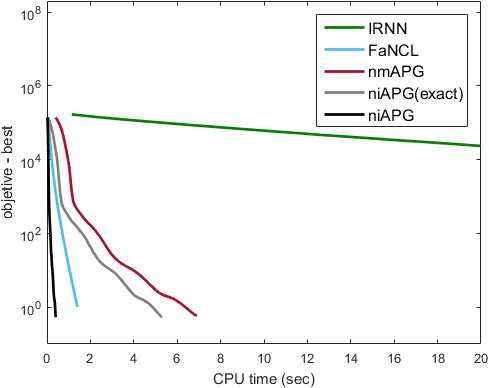
(a) $m=1000$.

(b) $m=2000$.

Figure 3: Objective value vs CPU time on the synthetic matrix completion data set.

Finally, we perform experiments on the large Netflix and Yahoo data sets (Table 6). We randomly use $50\%$ of the observed ratings for training, $25\%$ for validation and the rest for testing. Each experiment is repeated five times. We do not compare with nuclear-norm-regularized methods as they yield higher rank and RMSE than others. Table 7 shows the recovery performance, and Figures 2(b), 2(c) show the convergence. Again, niAPG is the fastest and most accurate.

Table 7: Results on the Netfix and Yahoo data sets. Here, RMSE is scaled by $\times 10^{-1}$.

		RMSE	rank	CPU time (min)
Netflix	AltGrad	8.16$\pm$0.02	15	221.7$\pm$5.6
	FaNCL	7.94$\pm$0.01	13	240.8$\pm$22.7
	nmAPG	7.92$\pm$0.01	13	132.8$\pm$2.1
	niAPG(exact)	7.92$\pm$0.01	13	97.7$\pm$1.8
	niAPG	7.92$\pm$0.01	13	25.2$\pm$0.6
Yahoo	AltGrad	6.69$\pm$0.01	14	112.9$\pm$4.2
	FaNCL	6.54$\pm$0.01	9	487.6$\pm$32.0
	nmAPG	6.53$\pm$0.01	9	184.3$\pm$6.3
	niAPG(exact)	6.53$\pm$0.01	9	140.7$\pm$5.8
	niAPG	6.53$\pm$0.01	9	38.7$\pm$2.3

6 Conclusion

In this paper, we proposed an efficient accelerated proximal gradient algorithm for nonconvex problems. Compared with the state-of-the-art Li and Lin (2015), the proximal step can be inexact and the number of proximal steps required is significantly reduced, while still ensuring convergence to a critical point. Experiments on image denoising and matrix completion problems show that the proposed algorithm has comparable (or even better) prediction performance as the state-of-the-art, but is much faster.

Appendix A Proof

A.1 Proposition 3.2

From Proposition 3.1, if the proximal step is exact at Algorithm 2, we have

$$F(x_{k+1})\leq F(v_{k})-\frac{\rho-L}{2}\|x_{k+1}-v_{k}\|_{2}^{2}.$$

Due to the condition at step 5, two cases are considered. Let $\alpha=\rho-L$, then

• If $v_{k}=x_{k}$, then $\Delta_{k}<F(y_{k})$ and

  $$F(x_{k+1}) \leq F(x_{k})-\frac{\alpha}{2}\|x_{k+1}-x_{k}\|_{2}^{2}$$

  $$\leq\Delta_{k}-\frac{\alpha}{2}\|x_{k+1}-x_{k}\|_{2}^{2}.$$ (9)

• If $v_{k}=y_{k}$, then $F(y_{k})\leq\Delta_{k}$ and

  $$F(x_{k+1})\leq F(y_{k})-\frac{\alpha}{2}\|x_{k+1}-y_{k}\|_{2}^{2}$$ (10)

By combining (9) and (10), we have

$$F(x_{k+1})\leq\min(F(y_{k}),\Delta_{k})-\frac{\alpha}{2}\|x_{k+1}-y_{k}\|_{2}^{2}.$$

A.2 Proposition 3.3

Let $\varsigma(w)=(w-v_{k})^{\top}\nabla f(v_{k})+\frac{\rho}{2}\|w-v_{k}\|_{2}^{2}+g(w)$. We have

$$\hat{x} = \arg\min_{w}h_{\frac{1}{\rho}g}(w)=\arg\min_{w}\varsigma(w),$$ (11)

$$\varsigma(w) = \rho h_{\frac{1}{\rho}g}(w)-\frac{1}{\rho}\|\nabla f(v_{k})\|_{2}^{2}.$$ (12)

From (11), we have

$$\varsigma(\hat{x}) =\langle\hat{x}-v_{k},\nabla f(v_{k})\rangle+\frac{\rho}{2}\|\hat{x}-v_{k}\|_{2}^{2}+g(\hat{x})$$

$$\leq g(v_{k}).$$ (13)

As $h_{\frac{1}{\rho}g}(x_{k+1})-h_{\frac{1}{\rho}g}(\hat{x})\leq\varepsilon_{k}$, from (12) (note that $\|\nabla f(v_{k})\|_{2}^{2}$ is a constant), we have

$$\varsigma(x_{k+1})-\varsigma(\hat{x})=\rho(h(x_{k+1})-h(\hat{x}))\leq\rho\epsilon$$

With (13), we have $\varsigma(x_{k+1})\leq\rho\varepsilon_{k}+\varsigma(\hat{x})\leq g(v_{k})+\rho\varepsilon_{k}$, and then

$$(x_{k+1}-v_{k})^{\top}\nabla f(v_{k}) +\frac{\rho}{2}\|x_{k+1}-v_{k}\|_{2}^{2}+g(x_{k+1})$$

$$\leq g(v_{k})+\rho\varepsilon_{k}.$$ (14)

As $f$ is $L$-Lipschitz smooth,

$$f(x_{k+1})\leq f(v_{k})+(x_{k+1}-v_{k})^{\top}\nabla f(v_{k})+\frac{L}{2}\|x_{k+1}-v_{k}\|_{2}^{2}.$$

Combining with (14), we obtain

$$f(x_{k+1})+\frac{\rho}{2}\|x_{k+1}-v_{k}\|_{2}^{2}+g(x_{k+1})$$

$$\leq f(v_{k})+\frac{L}{2}\|x_{k+1}-v_{k}\|_{2}^{2}+g(v_{k})+\rho\varepsilon_{k}.$$

Thus, $F(x_{k+1})\leq F(v_{k})-\frac{\rho-L}{2}\|x_{k+1}-v_{k}\|_{2}^{2}+\rho\varepsilon_{k}$.

A.3 Theorem 4.1

We first introduce one proposition.

Proposition A.1.

Let $\phi(k)=\arg\min_{t=\max(1,k-q),\dots,k}\|x_{t+1}-v_{t}\|_{2}^{2}$, then $\Delta_{k+q+1}\leq\Delta_{k}-\frac{\rho-L}{2}\|x_{\phi(k)+1}-v_{\phi(k)}\|_{2}^{2}$.

Proof.

From Proposition 3.2, we have

$$F(x_{k+1}) \leq\min\left(F(y_{k}),\Delta_{k}\right)-\frac{\rho-L}{2}\|x_{k+1}-v_{k}\|_{2}^{2}$$

$$\leq\Delta_{k}-\frac{\rho-L}{2}\|x_{k+1}-v_{k}\|_{2}^{2}.$$

Thus, $F(x_{k+1})\leq\Delta_{k}$. Then

$$F(x_{k+2}) \leq\Delta_{k+1}-\frac{\rho-L}{2}\|x_{k+2}-v_{k+1}\|_{2}^{2}$$

$$\leq\max(F(x_{k+1}),\Delta_{k})-\frac{\rho-L}{2}\|x_{k+2}-v_{k+1}\|_{2}^{2}$$

$$\leq\Delta_{k}-\frac{\rho-L}{2}\|x_{k+2}-v_{k+1}\|_{2}^{2}.$$

Inducting for $t=0,\dots,q$, we have

$$F(x_{k+1+t})\leq\Delta_{k}-\frac{\rho-L}{2}\|x_{k+1+t}-v_{k+t}\|_{2}^{2}.$$

Recall that $\Delta_{k}=\max_{t=k-q,\dots,k}F(x_{t})$, thus

$$\Delta_{k+q+1} =\max_{t=k+1,\dots,k+1+q}F(x_{t})$$

$$\leq\Delta_{k}-\min_{t=k,\dots,k+1}\frac{\rho-L}{2}\|x_{t+1}-v_{t}\|_{2}^{2}.$$

Let $\phi(k)=\arg\min_{t=k,\dots,k+q}\|x_{t+1}-v_{t}\|_{2}^{2}$, and then we get the proposition. ∎

Summing over $k=1,\dots,K$, then

$$\sum_{t=0}^{q} \Delta_{t+1}-\Delta_{K+t-q+1}$$

$$\geq\frac{\rho-L}{2}\sum_{k=1}^{K}\|x_{\phi(k)+1}-v_{\phi(k)}\|_{2}^{2}.$$ (15)

As $\inf F>-\infty$, let $K\rightarrow\infty$, then

$$\sum_{t=0}^{q}\Delta_{t+1}-\Delta_{K+t-q+1} \leq\sum_{t=0}^{q}(\Delta_{t+1}-\inf F)$$ (16)

$$\leq(q+1)\left(\max_{t=1,\dots,q+1}F(x_{t})-\inf F\right)$$

Let $c_{1}=(q+1)\left(\max_{t=1,\dots,q+1}F(x_{t})-\inf F\right)$, and it is easy to see $c_{1}<\infty$ is a finite number. Thus, from (15), we have

$$\lim_{k\rightarrow\infty}\|x_{\phi(k)+1}-v_{\phi(k)}\|_{2}=0,$$ (17)

which means $\lim_{k\rightarrow\infty}x_{\phi(k)+1}=v_{\phi(k)}$, and both sequence $\{x_{k}\}$ and $\{v_{k}\}$ are bounded, and then both have at least one limit point.

Let $\{v_{k_{j}}\}$ be a subsequence of $\{v_{k_{j}}\}$ and $x_{*}=\lim_{j\rightarrow\infty}x_{k_{j}+1}=\lim_{k_{j}\rightarrow\infty}v_{k_{j}}$ be a limit point, then

$$\lim_{k_{j}\rightarrow\infty}x_{k_{j}+1} =\lim_{j\rightarrow\infty}v_{k_{j}}$$

$$=\lim_{j\rightarrow\infty}\text{prox}_{\eta g}(v_{k_{j}}-\eta\nabla f(v_{k_{j}}))=x_{*}.$$

Besides, as $x_{k_{j}+1}$ is generated from proximal step on $v_{k_{j}}$, then

$$(x_{k_{j}+1}-v_{k_{j}})^{\top}\nabla f(v_{k_{j}})+\frac{\rho}{2}\|x_{k_{j}+1}-v_{k_{j}}\|_{2}^{2}+g(x_{k_{j}+1})$$

$$\leq(x_{*}-v_{k_{j}})^{\top}\nabla f(v_{k_{j}})+\frac{\rho}{2}\|x_{*}-v_{k_{j}}\|_{2}^{2}+g(x_{*})$$

Thus,

$$\lim_{j\rightarrow\infty}\sup g(x_{k_{j}+1})\leq g(x_{*}).$$ (18)

As $g$ is lower semicontinuous, we have

$$\lim_{k_{j}\rightarrow\infty}g(x_{k_{j}+1})\geq g(x_{*}).$$ (19)

Combining (18) and (19), we have

$$\lim_{k_{j}\rightarrow\infty}F(x_{k_{j}+1})=F(x_{*}),$$

and then with Lemma 4.2, $x_{*}$ is a critical point of (1).

A.4 Proposition 4.3

Note that $\mathcal{G}(v_{\phi(k)})=x_{\phi(k)+1}-v_{\phi(k)}$. Using (17), we have

$$\lim_{k\rightarrow\infty}\|\mathcal{G}(v_{\phi(k)})\|_{2}^{2}=0.$$

Then, using (15) and (16), we have

$$\sum_{k=1}^{K}\|x_{\phi(k)+1}-v_{\phi(k)}\|_{2}^{2}\leq\frac{2c_{1}}{\rho-L}$$

Thus,

$$\min_{k=1,\dots,K}\|\mathcal{G}(v_{\phi(k)})\|_{2}^{2}$$

$$=\min_{k=1,\dots,K}\|x_{\phi(k)+1}-v_{\phi(k)}\|_{2}^{2}$$

$$\leq\frac{1}{K}\sum_{k=1}^{K}\|x_{\phi(k)+1}-v_{\phi(k)}\|_{2}^{2}\leq\frac{2c_{1}}{(\rho-L)K}.$$

A.5 Theorem 4.4

We first extend Proposition A.1 to Proposition A.2 here.

Proposition A.2.

$\Delta_{k+q+1}\leq\Delta_{k}-\frac{\rho-L}{2}\|x_{\phi(k)+1}-v_{\phi(k)}\|_{2}^{2}+\rho\sum_{t=k}^{k+q}\varepsilon_{t}$.

Proof.

From Proposition 3.3, we have

$$F(x_{k+1}) \leq\min\left(F(y_{k}),\Delta_{k}\right)-\frac{\rho-L}{2}\|x_{k+1}-v_{k}\|_{2}^{2}+\rho\varepsilon_{k}$$

$$\leq\Delta_{k}-\frac{\rho-L}{2}\|x_{k+1}-v_{k}\|_{2}^{2}+\rho\varepsilon_{k}.$$

Thus, $F(x_{k+1})\leq\Delta_{k}+\rho\varepsilon_{k}$. Then

$$F(x_{k+2})$$

$$\leq\Delta_{k+1}-\frac{\rho-L}{2}\|x_{k+2}-v_{k+1}\|_{2}^{2}+\rho\varepsilon_{k+1}$$

$$\leq\max(F(x_{k+1}),\Delta_{k})-\frac{\rho-L}{2}\|x_{k+2}-v_{k+1}\|_{2}^{2}+\rho\varepsilon_{k+1}$$

$$\leq\Delta_{k}-\frac{\rho-L}{2}\|x_{k+2}-v_{k+1}\|_{2}^{2}+\sum_{t=k}^{k+1}\varepsilon_{t}.$$

Inducting for $t=0,\dots,q$, we have

$$F(x_{k+1+t})\leq\Delta_{k}-\frac{\rho-L}{2}\|x_{k+1+t}-v_{k+t}\|_{2}^{2}+\rho\sum_{t=k}^{k+q}\varepsilon_{t}.$$

Recall that $\Delta_{k}=\max_{t=k-q,\dots,k}F(x_{t})$, then

$$\Delta_{k+q+1} =\max_{t=k+1,\dots,k+1+q}F(x_{t})$$

$$\leq\Delta_{k}-\min_{t=k,\dots,k+1}\frac{\rho-L}{2}\|x_{t+1}-v_{t}\|_{2}^{2}+\rho\sum_{t=k}^{k+q}\varepsilon_{t}.$$

Thus, we get the proposition. ∎

Using Proposition A.2, sum over $k=1,\dots,K$, we have

$$\sum_{t=0}^{q}\Delta_{t+1}-\Delta_{K+t-q+1}$$

$$\geq\frac{\rho-L}{2}\sum_{k=1}^{K}\|x_{\phi(k)+1}-v_{\phi(k)}\|_{2}^{2}-\rho\sum_{t=k}^{\min(k+q,K)}\varepsilon_{t}$$

$$\geq\frac{\rho-L}{2}\sum_{k=1}^{K}\|x_{\phi(k)+1}-v_{\phi(k)}\|_{2}^{2}-\rho\sum_{t=k}^{k+q}\varepsilon_{t}$$

$$\geq\frac{\rho-L}{2}\sum_{k=1}^{K}\|x_{\phi(k)+1}-v_{\phi(k)}\|_{2}^{2}-q\rho\sum_{k=1}^{K}\varepsilon_{k}$$

$$\geq\frac{\rho-L}{2}\sum_{k=1}^{K}\|x_{\phi(k)+1}-v_{\phi(k)}\|_{2}^{2}-q\rho c.$$ (20)

where the last inequality comes from $\sum_{k=1}^{\infty}\varepsilon_{k}\leq c$, thus

$$\sum_{k=1}^{K}\|x_{\phi(k)+1}-v_{\phi(k)}\|_{2}^{2}$$

$$\leq\frac{2}{\rho-L}\sum_{t=0}^{q}\left(\Delta_{t+1}-\Delta_{K+t-q+1}+\rho c\right)$$

$$\leq\frac{2}{\rho-L}\sum_{t=0}^{q}\left(\Delta_{t+1}-\inf F+\rho c\right)$$

$$\leq\frac{2}{\rho-L}\sum_{t=0}^{q}\left(F(x_{1})-\inf F+\rho c\right).$$ (21)

Let $c_{2}=F(x_{1})-\inf F+\rho c$. As $c_{2}<\infty$, then

$$\lim_{k\rightarrow\infty}\|x_{\phi(k)+1}-v_{\phi(k)}\|_{2}=0,$$ (22)

which means $\lim_{k\rightarrow\infty}x_{\phi(k)+1}=v_{\phi(k)}$, and both sequence $\{x_{k}\}$ and $\{v_{k}\}$ are bounded and both have at least one limit point.

Let $x_{*}$ be a limit point, and $\{v_{k_{j}}\}$ be a subsequence of $\{v_{k}\}$ such that $\lim_{k_{j}\rightarrow\infty}x_{k_{j}+1}=\lim_{j\rightarrow\infty}v_{k_{j}}=x_{*}$. As $\lim_{k_{j}\rightarrow\infty}\varepsilon_{k_{j}}=0$, on step 11 of Algorithm 2, we have

$$\lim_{k_{j}\rightarrow\infty}x_{k_{j}+1} =\lim_{k_{j}\rightarrow\infty}\text{inexact }\text{prox}_{\eta g}(z_{k_{j}})$$

$$=\lim_{k_{j}\rightarrow\infty}\text{prox}_{\eta g}(z_{k_{j}}),$$

$$=\lim_{k_{j}\rightarrow\infty}\text{prox}_{\eta g}(v_{k_{j}}-\eta\nabla f(v_{k_{j}})),$$

which shows

$$x_{*}=\text{prox}_{\eta g}(x_{*}-\eta\nabla f(x_{*})).$$ (23)

As $g$ is convex and $f$ is Lipschitz-smooth, $F$ is continuous, then

$$\lim_{k_{j}\rightarrow\infty}F(x_{k_{j}})=F(x_{*}).$$

Thus, $x_{*}$ is also a critical point of (1) (Lemma 4.2).

A.6 Proposition 4.5

Let $v^{*}_{\phi(k)}=\text{prox}_{\eta g}(v_{\phi(k)}-\eta\nabla f(v_{\phi(k)}))$. Note that $h_{\eta g}(x)$ is $1$-strongly convex and $0\in\partial h_{\eta g}(v^{*}_{\phi(k)})$, thus

$$h(x_{\phi(k)+1})\geq h(v^{*}_{\phi(k)})+\frac{1}{2}\|x_{\phi(k)+1}-v^{*}_{\phi(k)}\|_{2}^{2}.$$

As $h(x_{\phi(k)+1})-h(v^{*}_{\phi(k)})\leq\varepsilon_{\phi(k)}$, thus $\|e_{\phi(k)}\|_{2}^{2}\equiv\|x_{k+1}-v^{*}_{\phi(k)}\|_{2}^{2}\leq 2\varepsilon_{\phi(k)}$.

A.7 Proposition 4.6

As $\mathcal{G}(v_{\phi(k)})+e_{k}=x_{\phi(k)+1}-v_{\phi(k)}$, thus

$$\|\mathcal{G}(v_{\phi(k)})\|_{2}^{2}\leq 2\left(\|x_{\phi(k)+1}-v_{\phi(k)}\|_{2}^{2}+\|e_{k}\|_{2}^{2}\right).$$

Combining Proposition 4.5 and (22), we have

$$\lim_{k\rightarrow\infty}\|\mathcal{G}(v_{\phi(k)})\|_{2}^{2}=0.$$

Besides, using (21) and $\sum_{k}^{\infty}\varepsilon_{k}\leq c$

$$\min_{k=1,\dots,K}\|\mathcal{G}(v_{\phi(k)})\|_{2}^{2}$$

$$\leq\frac{2}{K}\sum_{k=1}^{K}\left(\|x_{\phi(k)+1}-v_{\phi(k)}\|_{2}^{2}+\|e_{k}\|_{2}^{2}\right)$$

$$\leq\frac{2}{K}\sum_{k=1}^{K}\left(\|x_{\phi(k)+1}-v_{\phi(k)}\|_{2}^{2}+2\varepsilon_{\phi(k)}\right)$$

$$\leq\frac{2}{K}\left[4c+\frac{1}{\rho-L}\sum_{t=0}^{q}\left(F(x_{1})-\inf F+\rho c\right)\right].$$ (24)

As $c_{1}=\max_{t=1,\dots,q+1}F(x_{t})-\inf F$, then (24) can be simplified as

$$\min_{k=1,\dots,K}\|\mathcal{G}(v_{\phi(k)})\|_{2}^{2}\leq\frac{2}{K}\left[4c+\frac{(q+1)(c_{1}+\rho c)}{\rho-L}\right].$$

A.8 Theorem 4.7

Similar as Proposition A.1, we can obtain Proposition A.3 here, of which proof can also be done following Proposition A.1.

Proposition A.3.

$\Delta_{k+q+1}\leq\Delta_{k}-\frac{\delta}{2}\|x_{\phi(k)+1}-v_{\phi(k)}\|_{2}^{2}$.

Summing over $k=1,\dots,K$, then

$$\sum_{t=0}^{q}\Delta_{t+1}-\Delta_{K+t-q+1}\geq\frac{\delta}{2}\sum_{k=1}^{K}\|x_{\phi(k)+1}-v_{\phi(k)}\|_{2}^{2}.$$ (25)

As $\inf F>-\infty$, let $K\rightarrow\infty$, then

$$\sum_{t=0}^{q}\Delta_{t+1}-\Delta_{K+t-q+1} \leq\sum_{t=0}^{q}(\Delta_{t+1}-\inf F)$$ (26)

$$\leq(q+1)c_{1}.$$

As $c_{1}<\infty$ is a finite number, from (25), we have

$$\lim_{k\rightarrow\infty}\|x_{\phi(k)+1}-v_{\phi(k)}\|_{2}=0,$$ (27)

which means $\lim_{k\rightarrow\infty}x_{\phi(k)+1}=v_{\phi(k)}$, and both sequence $\{x_{k}\}$ and $\{v_{k}\}$ are bounded and both have at least one limit point.

A.9 Corollary 4.8

Let $x_{*}$ be a limit point, and $\{x_{k_{j}}\}$ be a subsequence of $\{x_{k}\}$ such that

$$\lim_{k_{j}\rightarrow\infty}x_{k_{j}+1}=\lim_{k_{j}\rightarrow\infty}v_{k_{j}}=x_{*}.$$

Next, we show that

$$x_{*}=\text{prox}_{\eta}(x_{*}-\nabla f(x_{*})).$$ (28)

We will prove it by establishing contradictory. Assuming (28) does not hold, then $x_{*}\neq\text{prox}_{\eta}(x_{*}-\eta\nabla f(x_{*}))$, and we can find another

$$\tilde{x}_{*}=\lim_{k_{j}\rightarrow\infty}x_{k_{j}+1}=\lim_{k_{j}\rightarrow\infty}\text{inexact }\text{prox}_{\eta g}(z_{k_{j}})\neq x_{*}$$

by Assumption (i), which is in contradiction with $\lim_{k_{j}\rightarrow\infty}x_{k_{j}+1}=x_{*}$. As a result, we have

$$x_{*}=\lim_{k_{j}\rightarrow\infty}x_{k_{j}+1} =\lim_{k_{j}\rightarrow\infty}\text{inexact }\text{prox}_{\eta g}(z_{k_{j}})$$

$$=\lim_{k_{j}\rightarrow\infty}\text{prox}_{\eta g}(z_{k_{j}})$$

$$=\lim_{k_{j}\rightarrow\infty}\text{prox}_{\eta g}(v_{k_{j}}-\eta\nabla f(v_{k_{j}}))$$

$$=\text{prox}_{\eta}(x_{*}-\eta\nabla f(x_{*})).$$

Besides, by Assumption (ii) we have

$$\lim_{k_{j}\rightarrow\infty}F(x_{k_{j}})=F(x_{*}).$$

Using Lemma 4.2 and (28), $x_{*}$ is a critical point of (1).

A.10 Proposition 4.10

Using (27), we have

$$\lim_{k\rightarrow\infty}\|x_{\phi(k)+1}-v_{\phi(k)}\|_{2}^{2}=0.$$

Finally, using (25) and (26), we have

$$\min_{k=1,\dots,K}\sum_{k=1}^{K}\|x_{\phi(k)+1}-v_{\phi(k)}\|_{2}^{2}$$

$$\leq\frac{1}{K}\sum_{k=1}^{K}\|x_{\phi(k)+1}-v_{\phi(k)}\|_{2}^{2}$$

$$\leq\frac{2}{\delta K}\sum_{t=0}^{q}\left(F(x_{1})-\inf F\right)=\frac{2(q+1)c_{1}}{\delta K}.$$

References

- Attouch et al. [2013] H. Attouch, J. Bolte, and B.F. Svaiter. Convergence of descent methods for semi-algebraic and tame problems: Proximal algorithms, forward-backward splitting, and regularized Gauss-Seidel methods. Mathematical Programming, 137(1-2):91–129, 2013.
- Beck and Teboulle [2009a] A. Beck and M. Teboulle. Fast gradient-based algorithms for constrained total variation image denoising and deblurring problems. IEEE Transactions on Image Processing, 18(11):2419–2434, 2009.
- Beck and Teboulle [2009b] A. Beck and M. Teboulle. A fast iterative shrinkage-thresholding algorithm for linear inverse problems. SIAM Journal on Imaging Sciences, 2(1):183–202, 2009.
- Boyd et al. [2011] S. Boyd, N. Parikh, E. Chu, B. Peleato, and J. Eckstein. Distributed optimization and statistical learning via the alternating direction method of multipliers. Foundations and Trends in Machine Learning, 3(1):1–122, 2011.
- Candès et al. [2008] E.J. Candès, M.B. Wakin, and S. Boyd. Enhancing sparsity by reweighted minimization. Journal of Fourier Analysis and Applications, 14(5-6):877–905, 2008.
- Ghadimi and Lan [2015] S. Ghadimi and G. Lan. Accelerated gradient methods for nonconvex nonlinear and stochastic programming. Mathematical Programming, 156(1-2):1–41, 2015.
- Gong et al. [2013] P. Gong, C. Zhang, Z. Lu, J. Huang, and J. Ye. A general iterative shrinkage and thresholding algorithm for non-convex regularized optimization problems. In ICML, pages 37–45, 2013.
- Grippo and Sciandrone [2002] L. Grippo and M. Sciandrone. Nonmonotone globalization techniques for the Barzilai-Borwein gradient method. Computational Optimization and Applications, 23(2):143–169, 2002.
- Halko et al. [2011] N. Halko, P.G. Martinsson, and J.A. Tropp. Finding structure with randomness: Probabilistic algorithms for constructing approximate matrix decompositions. SIAM Review, 53(2):217–288, 2011.
- Hastie et al. [2015] T. Hastie, R. Mazumder, J.D. Lee, and R. Zadeh. Matrix completion and low-rank SVD via fast alternating least squares. Journal of Machine Learning Research, 16:3367–3402, 2015.
- Hsieh and Olsen [2014] C.J. Hsieh and P. Olsen. Nuclear norm minimization via active subspace selection. In ICML, pages 575–583, 2014.
- Larsen [1998] R.M. Larsen. Lanczos bidiagonalization with partial reorthogonalization. DAIMI PB-357, Department of Computer Science, Aarhus University, 1998.
- Li and Lin [2015] H. Li and Z. Lin. Accelerated proximal gradient methods for nonconvex programming. In NIPS, pages 379–387, 2015.
- Lu et al. [2014] C. Lu, J. Tang, S Yan, and Z Lin. Generalized nonconvex nonsmooth low-rank minimization. In CVPR, pages 4130–4137, 2014.
- Nesterov [2004] Y. Nesterov. Introductory Lectures on Convex Optimization: A Basic Course. Springer, 2004.
- Nesterov [2013] Y. Nesterov. Gradient methods for minimizing composite functions. Mathematical Programming, 140(1):125–161, 2013.
- Ochs et al. [2014] P. Ochs, Y. Chen, T. Brox, and T. Pock. iPiano: Inertial proximal algorithm for nonconvex optimization. SIAM Journal on Imaging Sciences, 7(2):1388–1419, 2014.
- Parikh and Boyd [2014] N. Parikh and S. Boyd. Proximal algorithms. Foundations and Trends in Optimization, 1(3):127–239, 2014.
- Schmidt et al. [2011] M. Schmidt, N.L. Roux, and F. Bach. Convergence rates of inexact proximal-gradient methods for convex optimization. In NIPS, pages 1458–1466, 2011.
- Wang et al. [2015] Z. Wang, M.J. Lai, Z. Lu, W. Fan, H. Davulcu, and J. Ye. Orthogonal rank-one matrix pursuit for low rank matrix completion. SIAM Journal on Scientific Computing, 37(1), 2015.
- Wright et al. [2009] S.J. Wright, R.D. Nowak, and M.A. Figueiredo. Sparse reconstruction by separable approximation. IEEE Transactions on Signal Processing, 57(7):2479–2493, 2009.
- Yao and Kwok [2016] Q. Yao and J.T. Kwok. Efficient learning with a family of nonconvex regularizers by redistributing nonconvexity. In ICML, pages 2645–2654, 2016.
- Yao et al. [2015] Q. Yao, J.T. Kwok, and W. Zhong. Fast low-rank matrix learning with nonconvex regularization. In ICDM, pages 539–548, 2015.
- Yuille and Rangarajan [2002] A.L. Yuille and A. Rangarajan. The concave-convex procedure (CCCP). In NIPS, pages 1033–1040, 2002.
- Zhang et al. [2012] X. Zhang, D. Schuurmans, and Y.-L. Yu. Accelerated training for matrix-norm regularization: a boosting approach. In NIPS, pages 2906–2914, 2012.
- Zhang [2010] T. Zhang. Analysis of multi-stage convex relaxation for sparse regularization. Journal of Machine Learning Research, 11:1081–1107, 2010.
- Zhao et al. [2015] T. Zhao, Z. Wang, and H. Liu. A nonconvex optimization framework for low rank matrix estimation. In NIPS, pages 559–567, 2015.
- Zhong and Kwok [2014] L.W. Zhong and J.T. Kwok. Gradient descent with proximal average for nonconvex and composite regularization. In AAAI, pages 2206–2212, 2014.