Off-site trimer superfluid on a one-dimensional optical lattice

Abstract

The Bose-Hubbard model with an effective off-site three-body tunneling, characterized by jumps towards one another, between one atom on a site and a pair atoms on the neighborhood site, is studied systematically on a one-dimensional lattice, by using the density matrix renormalization group method. The off-site trimer superfluid, condensing at momentum $k=0$, emerges in the softcore Bose-Hubbard model but it disappears in the hardcore Bose-Hubbard model. Our results numerically verify that the off-site trimer superfluid phase derived in the momentum space from [Phys. Rev. A 81, 011601(R) (2010)] is stable in the thermodynamic limit. The off-site trimer superfluid phase, the partially off-site trimer superfluid phase and the Mott insulator phase are found, as well as interesting phase transitions, such as the continuous or first-order phase transition from the trimer superfluid phase to the Mott insulator phase. Our results are helpful in realizing this novel off-site trimer superfluid phase by cold atom experiments.

I introduction

Exploring the novel phases of cold atom systems is an important guide in understanding the collective behavior of the quantum many-body system. The optical lattice opt1 ; opt2 ; opt3 provides us an ideal and perfect platform hosting the cold atoms, described by the Bose-Hubbard (BH) model.djak ; mgre Interestingly, various kinds of novel quantum phases, such as the atom superfluid (ASF) phase,sf1 ; sf2 the pair SF (PSF) phase or the trimer SF (TSF) phase, emerge on the optical lattices, by controlling laser as well as other various parameters. Also there are interesting mixed phases, such as the partially paired superfluid phase.pp ; ppphase

In the ASF phase, one atom jumps repeatedly to its neighboring sites. In the PSF phase, a pair of atoms are able to tunnel simultaneously from one site to the neighborhood sites, driven by the attractive interaction,cqst5 ; cqst6 ; thermal or laser-assisted to the state dependent optical latice.xfzhou Another type of PSF phase is characterized by a jump of the off-site pair atoms, from the sites $i$ and $j$ to another two sites labeled $k$ and $l$.hcjiang ; corre In spin language, the off-site pair tunneling can be represented in the spin-$\frac{1}{2}$ XY model with four-spin interactions.s12 ; fourspin ; fspin

Naturally, the question arises: can the off-site trimer superfluid(OTSF) exist in a stable fashion? In the OTSF phase, a trimer is composed of one atom on a site and the other two atoms on the neighborhood site.

Fortunately, the derivation of the Hamiltonian with an effective off-site trimer model in Ref. central , shows that the off-site trimer model exists probably in theory. Moreover, condensation of the off-site trimer on a kagomé latticezhaihui supports the existence of the OTSF phase in quantum many-body systems. Furthermore, experimental realization of local trimers, by using 7Li,li7 ; li7b ; li7c 39K,39K 85Rb85Rb and 133Cs,133Cs ; 133Csb and numerical studies of trimer-tunneling modelliran ; yangyuan are helpful in understanding the OTSF phase.

Herein, we use the density matrix renormalization group (DMRG) methoddmrg ; dmrg2 to study a BH model with off-site trimer tunneling on a one-dimensional optical lattice, and find that the OTSF phase derived in the momentum space from Ref. central exists in a stable fashion in the thermodynamic limit. This OTSF phase emerges in the softcore BH model though it disappears in the hardcore model. Interestingly, the partial OTSF (POTSF) phase, i.e. a phase mixed with the ASF and OTSF phases, is also found.

The outline of this work is as follows. Section II   shows the Hamiltonian model. Section III   describes the DMRG method and the useful observables. Section IV    studies both the hardcore and softcore BH models, and then finds out if the OTSF and POTSF phases exist in the softcore BH model, and the phase diagrams are also discussed. Concluding comments are made in Sec V.

II The Hamiltonian model

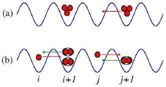
Figure 1: (color online) (a) A static trimer on the site labeled $i+1$ and an active trimer tunneling between $j$ and $j+1$. (b) An off-site trimer tunneling between $j$ and $j+1$ in the hardcore model with $n_{max}^{p}=1$ and an off-site trimer with a softcore model with $n_{max}^{p}=2$ between $i$ and $i+1$.

The starting point is the BH Hamiltonian with an off-site trimer tunneling term, as shown in Ref. central

$$H=H_{a}+H_{p}+H_{ap},$$ (1)

with

$$H_{a}= -J\sum_{i=1}^{L}\left(a_{i}^{\dagger}a_{i+1}+H.c.\right)+\sum_{i=1}^{L}h_{i}^{a},$$ (2)

where $J$ is the atom hopping rate, $a_{i}^{\dagger}$ ($a_{i}$) is the atom creation (annihilation) operator, the operator on each site is $h_{i}^{a}=\frac{U}{2}(n_{i}^{a}(n_{i}^{a}-1))-\mu_{a}n_{i}^{a}$ and $n_{i}^{a}=a_{i}^{\dagger}a_{i}$ is the occupation number operator at site $i$, $U$ is the on-site two-body interaction energy and $\mu_{a}$ is the chemical potential of atoms (for simplicity, we ignore the subscript “$a$” in this work). $H_{a}$ describes the single atom tunneling and the interactions between atoms.

The second term $H_{p}$ exhibits the tunneling and interactions between bounded pairs of atoms and is given by

$$H_{p}= -J_{p}\sum_{i=1}^{L}\left(p_{i}^{\dagger}p_{i+1}+H.c.\right)+\sum_{i=1}^{L}h_{i}^{p},$$ (3)

with $p_{i}^{\dagger}$ ($p_{i}$) being the pair (bound-particle pair) creation (annihilation) operator, $h_{i}^{p}=\frac{U}{2}(n_{i}^{p}(n_{i}^{p}-1))-\mu_{p}n_{i}^{p}$ and $n_{i}^{p}=p_{i}^{\dagger}p_{i}$ is the number operator of paired atoms at site $i$. The effective pair hopping is $J_{p}=-\frac{2J^{2}}{U}$,central and $\mu_{p}=U-2J_{p}$.

$H_{ap}$ describes the effective short-range interactions between the single atom and the paired atoms, as follows,

$$H_{ap}=V\sum_{i=1}^{L}n_{i}^{p}n_{i+1}^{a}-W\sum_{i=1}^{L}\left(p_{i}a_{i}^{\dagger}p_{i+1}^{\dagger}a_{i+1}+H.c.\right),$$ (4)

where $V=-\frac{7J^{2}}{2U}$ denotes a weak attractive nearest-neighbor interaction, and $W=2J$central is the off-site trimer tunneling energy, as shown in Fig. 1(b).

It should be noted that particles “a” and “p” are the same kind of atoms. Here, “a” denotes the single atom component and “p” represents the component of the paired atoms.

III Methods and order parameters

To explore the OTSF phase and get the reliable phase diagrams, we use the DMRG method dmrg ; dmrg2 ; dmrg3 to simulate the model described by Eq. (1) for a chain with a periodic boundary condition. In order to ensure the correctness of the DMRG method, we compare the ground state energies of the hardcore BH model with $n_{max}^{a}=n_{max}^{p}=1$ by the Lanczos and DMRG methods. The chosen parameters are $J/U=0.4$, $\mu/U=-0.5$, and the dimension of the truncated matrix takes $m=80\sim 130$ within the DMRG method. The results from both methods are completely the same within $10$ digits with $L=4,6,8,10$, and the first $5$ significant numbers are given in Tab. 1. While $L=12$, data from both methods are the same within $4$ digits. The consistency can be seen in Fig. 2(a).

The dimensions $m=80\sim 130$ of the truncated matrix are reliable to get the ground state of the Hamiltonian. The ground state energies versus $m$ with sizes $L=20$ and $48$ are shown in Fig. 2(b) and they are convergent when $m=80$. Furthermore, in the present work, the attractive interaction considers $V\textless 0$, and the number of possible phases is smaller than that with repulsive interaction, where various density wave (DW) phases emerge in the extended BH model on a one-dimensional optical lattice.dw1 ; dw2 ; dw3 Therefore, $m=80\sim 130$ is reasonable for the parameters with $V\textless 0$ and the results seem easier to converge.

Table 1: Values of the ground state energies by the Lanczos and DMRG methods with different sizes $L$.

	4	6	8	10	12
Lanczos	-2.18378	-2.20702	-2.22733	-2.24232	-2.25214
DMRG	-2.18378	-2.20702	-2.22733	-2.24232	-2.25212

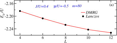
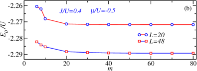
Figure 2: (color online) The ground state energies of the hardcore BH model with $n_{max}^{a}=n_{max}^{p}=1$ at $J/U=0.4$, $\mu/U=-0.5$ (a) by the Lanczos and DMRG methods with different sizes $L$. And in the DMRG method, the dimension of the truncated matrix takes $m=80\sim 130$. (b) The ground state energies versus $m$ with sizes $L=20$ and $48$.

The average correlation functionshcjiang are defined to distinguish each quantum phase as follows,

$$C_{a} =\frac{\sum_{r=1}^{L}C_{a}(r)}{L},C_{a}(r)=\langle a_{i}^{\dagger}a_{i+r}\rangle,$$ (5)

$$C_{p} =\frac{\sum_{r=1}^{L}C_{p}(r)}{L},C_{p}(r)=\langle p_{i}^{\dagger}p_{i+r}\rangle,$$

$$C_{ap} =\frac{\sum_{r=1}^{L}C_{ap}(r)}{L},C_{ap}(r)=\langle p_{i}^{\dagger}a_{i}a_{i+r}^{\dagger}p_{i+r}\rangle.$$

With finite sizes, the ASF phase is characterized by $C_{a}\neq 0$ and the OTSF phase is denoted by $C_{ap}$. For the POTSF phase, both $C_{a}$ and $C_{ap}$ are nonzero. Although the average correlation functions $C_{a}$, and $C_{ap}$ tend to be zero in the thermodynamic limit, i.e., $L\to\infty$, $\int_{0}^{L}C_{a}(r)/L=0$ and $\int_{0}^{L}C_{ap}(r)/L=0$, we can still use $C_{a}$, and $C_{ap}$ with the finite sizes to conveniently judge phase transitions. Finally, by $C_{a}(r)$ and $C_{ap}(r)$ described by algebraically or exponentially decaying functions, we can determine whether or not the novel phases really exist in the thermodynamic limit. The on-site interaction $U$ is taken as a unit $U=1$, and the chemical potential of pairs, i.e. $\mu_{p}=U-2J_{p}=U-2\times(-\frac{2J^{2}}{U})\textgreater 1$ is relatively larger. Hence, for both the hardcore or softcore models, the system sits in the MI phase, i.e., MI($\rho_{p}=1$) for the hardcore model and MI($\rho_{p}=2$) for the softcore model, where the quantities $C_{p}(r)$ and $C_{p}$ remain at zero, and therefore the pair momentum distribution $n_{p}(k)$ has no peak. Herein, we ignore the detailed discussion about the corresponding quantities ( $C_{p}(r)$, $C_{p}$ and $n_{p}(k)$).

Furthermore, the momentum distributions are also used to detect various SF phases and defined as momentum

$$n_{a}(k) =\frac{1}{L}\sum_{i,j}\langle a_{i}^{\dagger}a_{j}\rangle e^{ik(i-j)},$$ (6)

$$n_{p}(k) =\frac{1}{L}\sum_{i,j}\langle p_{i}^{\dagger}p_{j}\rangle e^{ik(i-j)},$$

$$n_{ap}(k) =\frac{1}{L}\sum_{i,j}\langle p_{i}^{\dagger}a_{i}a_{j}^{\dagger}p_{j}\rangle e^{ik(i-j)}.$$

The momentum distributions will have peaks for the three types SF phases. Specifically, $n_{a}(k)$ will peak at $k=0$ in the POTSF and ASF phases, and $n_{ap}(k)$ will peak at $k=0$ in the POTSF and OTSF phases.

Moreover, the integer fillings of the single atom component $\rho_{a}=\frac{\sum_{i=1}^{L}\langle n_{i}^{a}\rangle}{L}$ and the paired-atom component $\rho_{p}=\frac{\sum_{i=1}^{L}\langle n_{i}^{p}\rangle}{L}$ are also used to characterize the Mott insulator (MI) phase. In Tab. 2, we list the values of the order parameters for several typical phases, namely the OTSF, ASF and MI phases. The ASF phase means that the system sits in the SF_a+MI_p phase.

Table 2: Values of the order parameters $C_{a}$ and $C_{ap}$, and characteristics of $C_{a}(r)$, $C_{ap}(r)$, $n_{a}(k)$ and $n_{ap}(k)$ for typical phases. “$A$” and “$E$” denote $C_{a}(r)$ or $C_{ap}(r)$ obeys a decaying behavior, algebraically and exponentially, respectively. “$\surd$” means $n_{a}(k)$ or $n_{ap}(k)$ will peak at $k=0$.

	$C_{a}$	$C_{ap}$	$C_{a}(r)$	$C_{ap}(r)$	$n_{a}(k)$	$n_{ap}(k)$
POTSF	$\neq 0$	$\neq 0$	$A$	$A$	$\surd$	$\surd$
OTSF	0	$\neq 0$	$E$	$A$		$\surd$
ASF	$\neq 0$	0	$A$	$E$	$\surd$
MI	0	0	$E$	$E$

IV Results

IV.1 Hardcore off-site trimer BH model

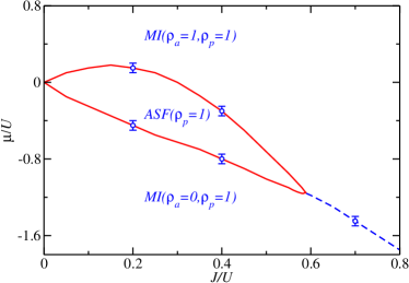
Figure 3: (color online) The hardcore phase diagram with $n_{max}^{a}=n_{max}^{p}=1$, which contains the MI($\rho_{a}=0$, $\rho_{p}=1$), ASF and MI($\rho_{a}=1$, $\rho_{p}=1$) phases in the plane ($J/U$, $\mu/U$). The lines are schematic phase boundaries. The dashed and solid lines denote the first order and continuous phase transitions, respectively.

Initially, we studied the hardcore BH model with the maximum occupation number $n_{max}^{a}=n_{max}^{p}=1$, where each site is only allowed to be occupied by one atom or a pair of atoms.

The phase diagram is shown in Fig. 3, where no OTSF phase exists and only the ASF and MI phases emerge. The system sits in the MI($\rho_{a}=0$, $\rho_{p}=1$) phase if $\mu/U\textless 0$, and the system enters into the MI($\rho_{a}=1$, $\rho_{p}=1$) phase when $\mu/U$ become larger. The ASF phase, i.e., the SF_a+MI_p phase exists in the middle of the phase diagram, and is similar to the SF_A+MI_B phase in Refsfmi . The phase transitions from the ASF phase to the MI phases are continuous as expected.

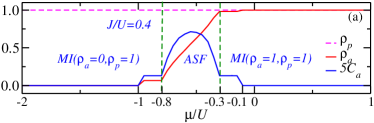
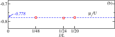
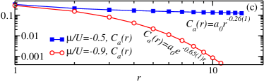
Figure 4: (color online) (a) The values of the densities $\rho_{a}$, $\rho_{p}$ and average correlation function $C_{a}$ along $\mu/U$ at $J/U=0.4$ with size $L=48$. (b) The phase transition point $\mu_{c}/U$ vs $1/L$ from the MI($\rho_{a}=0$, $\rho_{p}=1$) phase to the ASF phase. (c) Correlation $C_{a}(r)$ at $\mu/U=-0.9$ and $-0.5$.

For a more detailed description of the each physical quantity, we choose to scan $\mu/U$ at $J/U=0.4$ as shown in Fig. 4. In Fig. 4(a), when $\mu/U\textless-1$, the single-atom component sits in the empty phase, i.e., $\rho_{a}=0$. The paired-atom component sits in the MI phase, i.e., $\rho_{p}=1$. Due to the relationship,

$$\mu_{p}=U-2J_{p}=U-2\times(-\frac{2J^{2}}{U})\textgreater 1,$$ (7)

$\mu_{p}$ is relatively larger for the paired-atom component, and the system sits in the MI($\rho_{a}=0$, $\rho_{p}=1$) phase. In the range $-1\textless\mu/U\textless-0.8$, the system is still at the MI($\rho_{a}=0$, $\rho_{p}=1$) phase. The density $\rho_{a}\neq 0$ is due to the finite size effects, which are eliminated by finite size scaling. The scaling of $\rho_{a}$ with sizes $L=20,24,48$ at $\mu/U=-0.9$ is done and $\rho_{a}$ vanishes at the thermodynamic limit. For the sake of simplicity, the scaling is not shown here.

Similarly, in the range $-0.3\textless\mu/U\textless-0.1$, the system is in the MI ($\rho_{a}=1$, $\rho_{p}=1$) phase. In the range $-0.8\textless\mu/U\textless-0.3$, the system is in the ASF phase as $C_{a}\neq 0$ obviously.

In the plots of Fig. 4, we only show the results with size $L=48$, and one may therefore worry about the size effect causing the deviation of the phase transition point $\mu_{c}/U$ from the MI($\rho_{a}=0$, $\rho_{p}=1$) phase to the ASF phase. The finite size scaling of the transition points $\mu_{c}/U$ shows that the deviation is invisible, as shown in Fig. 4(b).

The finite size effects of $C_{a}\neq 0$ in both ranges $-1\textless\mu/U\textless-0.8$ and $-0.3\textless\mu/U\textless-0.1$ can be confirmed by the behaviors of $C_{a}(r)$. In Fig. 4(c), the exponentially decaying function $C_{a}(r)$ satisfying $C_{a}(r)=a_{0}e^{-0.65(1)r}$ at $\mu/U=-0.9$, shows that there is no superfluid order and the system sits in the MI($\rho_{a}=0$, $\rho_{p}=1$) phase.decay1 ; decay2 While at $\mu/U=-0.5$, the algebraically decaying function $C_{a}(r)$, namely $C_{a}(r)=a_{0}r^{-0.26(1)}$, tells us that the system is of a strong superfluid order and sits in the ASF phase.

In the whole range$-2\textless\mu/U\textless 1$, $\rho_{p}$ maintains itself at unity. The reason why is because $\mu_{p}$ is independent of $\mu$ and is a constant, which results in that the paired-atom component sits in the MI($\rho_{p}=1$) phase.

The system includes the single atom and the pair atoms coupling term $p_{i}a_{i}^{\dagger}p_{i+1}^{\dagger}a_{i+1}$ in Eq. (4). Compared to the usual hardcore BH model,hardcore the phase diagram is asymmetric about $\mu$.

IV.2 Softcore off-site trimer model

IV.2.1 The global phase diagram

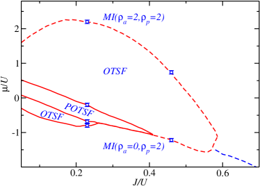
Figure 5: (color online) The softcore phase diagram $(J/U-\mu/U)$ with the maximum occupation number $n_{max}^{a}=n_{max}^{p}=2$. The lines are schematic phase boundaries. The dashed lines denote the first order phase transition, and the solid lines mark the continuous phase transition.

Since the OTSF phase doesn’t emerge in the hardcore model, and Ref. central found the OTSF phase in the softcore model, we will study the softcore BH model in this section, and expect to find the stable OTSF phase.

Fig. 5 shows the global phase diagram of the softcore BH model. When $\mu/U$ is very large or negative, the system sits in the MI($\rho_{a}=2$, $\rho_{p}=2$) and MI($\rho_{a}=0$, $\rho_{p}=2$) phases, respectively. Furthermore, in the regime where $J/U$ is relatively strong, the system is in the two phases. Fortunately, in contradistinction to the hardcore model, when the ratio $J/U$ becomes weaker, the expected OTSF phase appears and distributes into a large region. More interestingly, apart from the pure OTSF phase, a POTSF phase distributes between the two OTSF phases. In this parameter regime, the single atom tunneling and the off-site tunneling can exist simultaneously. In other words, a part of the OTSF phase is broken by the on-site repulsions, and becomes a normal SF phase, i.e., a POTSF phase. It is similar to the partially paired (PP) phase in the anyon Hubbard model.pp ; ppphase

Furthermore, the phase transitions between the OTSF phase and other phases are also interesting. The phase transition from the MI phase to the OTSF phase can be continuous or first order. When $J/U\textless 0.41$, it is continuous, and will turn into first order transition when $J/U\textgreater 0.41$. Moreover, the phase transition from the OTSF phase to the MI($\rho_{a}=2$, $\rho_{p}=2$) phase is the first order. Furthermore, it should be noted that the phase transition between the POTSF phase and the pure OTSF phase is still continuous. This phase transition is similar to the transition that from the PP phase to the SF or PSF phase in Ref. pp . All these phase transitions were not discussed in Ref. central .

IV.2.2 Detailed analysis

In order to analyze these phase transitions and give detailed descriptions of each physical quantity, we select $J/U=0.23$ and $0.46$ as examples, as shown in Figs. 6 and  7, respectively.

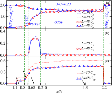
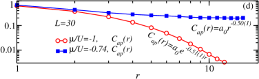
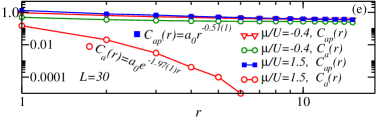
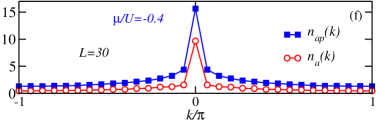
Figure 6: (color online) The values of the (a) densities $\rho_{a}$, $\rho_{p}$, (b) average correlation functions $C_{a}$, and (c) $C_{ap}$ vary with $\mu/U$ at $J/U=0.23$ with sizes $L=20$ and $48$. (d) $C_{ap}(r)$ at $\mu/U=-1$ and $-0.74$, (e) $C_{ap}(r)$ and $C_{a}(r)$ at $\mu/U=-0.4$ and $1.5$, (f) $n_{a}(k)$ and $n_{ap}(k)$ at $\mu/U=-0.4$ with sizes $L=30$.

In Fig. 6(a), when $\mu/U\textless-0.8$, the system sits in the MI($\rho_{a}=0$, $\rho_{p}=2$) phase. There is no single atom on the lattice, and every site is occupied by two pairs of atoms, i.e., four atoms. The reason why is because this scenario is similar to that of the hardcore model where $\mu_{p}$ is relatively large. In the range $-1.1\textless\mu/U\textless-0.8$, there is a platform of $C_{ap}$ in Fig. 6(c), $C_{ap}\neq 0$ with two finite sizes $L=20$ and $48$. However, It doesn’t mean that the system sits in the OTSF phase, due to $C_{ap}(r)$ obeying an exponentially decaying curve rather than an algebraically decaying curve in these parameter regimes, as shown at $\mu/U=-1$ in Fig. 6(d).

Continuously increasing $\mu/U$, in the narrow region $-0.8\textless\mu/U\textless-0.68$, an OTSF phase emerges, as $C_{ap}\neq 0$ obviously, confirmed by the algebraically decaying $C_{ap}(r)$ at $\mu/U=-0.74$ in Fig. 6(d). It should be noted that $C_{a}(r)$ is not shown here due to the fact that $C_{a}=0$. Moreover, the continuous variation of $C_{ap}$ implies that the phase transition from the MI($\rho_{a}=0$,$\rho_{p}=2$) phase to the OTSF phase is also continuous. Similarly, the OTSF phase also emerges in the region $-0.2\textless\mu/U\textless 2.2$. In Fig. 6(e), at $\mu/U=1.5$, the algebraically decaying $C_{ap}(r)$ and exponentially decaying $C_{a}(r)$ confirm that the system sits in a pure OTSF phase. Moreover, the quantity $C_{ap}$ jumps at $\mu/U=2.2$ in Fig. 6(c), with the implication that the phase transition between the OTSF phase and the MI($\rho_{a}=2$, $\rho_{p}=2$) phase is first order.foqpt1

Apart from the pure OTSF phase, a POTSF phase also emerges. In the range $-0.68\textless\mu/U\textless-0.2$, in Figs. 6(b) and (c), both $C_{a}$ and $C_{ap}$ are obviously nonzero, and both $C_{ap}(r)$ and $C_{a}(r)$ obey algebraically decaying functions, as shown in Fig. 6(e), at $\mu/U=-0.4$. The phase transition from the POTSF phase to the OTSF phase is continuous.

For cold atom experiments, the momentum distribution can be used to detect the novel POTSF phase. In Fig. 6(f), by a Fourier transformation of both $C_{ap}(r)$ and $C_{a}(r)$ according to Eq. (6), we can get the momentum distributions $n_{a}(k)$ and $n_{ap}(k)$, both of which have peaks at $k=0$, similar to the outcome of Ref. central . According to the characteristics of the momentum distributions in Table 2, the two peaks indicate that the system is indeed in the POTSF phase rather than any other phase.

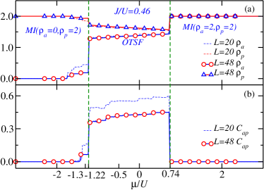
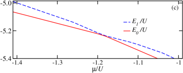
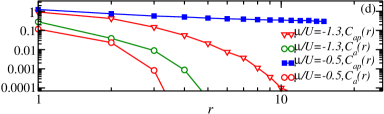
Figure 7: (color online) The values of the (a) densities $\rho_{a}$, $\rho_{p}$, (b) average correlation functions $C_{ap}$ vary with $\mu/U$ at $J/U=0.46$ with sizes $L=20$ and $48$. (c) $E_{1}/U$ and $E_{0}/U$ mean dimensionless excited and ground states energies, respectively, from the MI($\rho_{a}=0$, $\rho_{p}=2$) phase to the OTSF phase by exact diagonalization with four lattice sites. (d) $C_{ap}(r)$ and $C_{a}(r)$ at $\mu/U=-1.3$ and $-0.5$ with sizes $L=30$ and $48$, respectively.

Apart from $J/U=0.23$, the details concerning $J/U=0.46$ are discussed and $\rho_{a}$, $\rho_{p}$ and $C_{ap}$ are shown by scanning $\mu/U$ in Figs. 7(a) and (b). Clearly, the phase transitions from the OTSF phase to both the MI($\rho_{a}=0$, $\rho_{p}=2$) or MI($\rho_{a}=2$, $\rho_{p}=2$) phases, satisfy the discontinuous change of a order parameter when a first-order phase transition takes place.foqpt1

To understand the first-order phase transition more intuitively, the excited and ground energies are also calculated by exact diagonalization with four lattice sites, as shown in Fig. 7(c), where an intersection emerges around $\mu/U=-1.22$, which is consistent with the phenomenon of coexistence between two phases at the critical phase transition point as the first-order phase transitionfoqpt2 occurs from the MI($\rho_{a}=0$, $\rho_{p}=2$) phase to the OTSF phase. A small deviation of this phase transition point is caused by the finite size effect.

In Fig. 7(b), near $\mu/U=-1.3$, $C_{ap}\neq 0$ for the two finite sizes $L=20$ and $48$ as $C_{ap}$ is a platform in the range $-1.1\textless\mu/U\textless-0.8$ in Fig. 6(c), yet we are still certain the system sits in the MI($\rho_{a}=0$, $\rho_{p}=2$) phase, based on the fact that $C_{ap}(r)$ and $C_{a}(r)$ obey exponentially decaying functions in this region, as shown at $\mu/U=-1.3$ in Fig. 7(d). Furthermore, when $\mu/U=-0.5$, the algebraically decaying $C_{ap}(r)$ and exponentially decaying $C_{a}(r)$ confirm that the system sits in a pure OTSF phase. The reason why $C_{a}$ is not shown in Figs. 7 is that $C_{a}(r)$ obeys exponential decay.

V Discussion and conclusion

By using the DMRG method, the BH model, with an effective off-site three-body tunneling and the attractive nearest-neighbor interaction, was studied on a one-dimensional optical lattice.

The OTSF phase and POTSF phases of the softcore BH model, is stable in the thermodynamic limit. The phase transition between the OTSF phase and the MI phase can be first order or continuous, depending on the parameters $J/U$ and $\mu/U$.

Our results numerically verify that the OTSF phase derived in the momentum space from Ref. central is stable in the thermodynamic limit. By using the DMRG method, we calculated the global phase diagrams and the interesting phase transitions. This is an important extension of the mean field work in Ref. central . The new results in this work concerning the OTSF and POTSF phases are helpful in realizing and understanding the novel phases by cold atom experiments.

References

- (1) Greiner M, Mandel O, Dsslinger T, Hänsch T W and Bloch I 2002 Nature 415 39
- (2) Greiner M and Föllin S 2008 Nature 453 736
- (3) Oosten D V, Straten P V D and Stoof H T C 2001 Phys. Rev. A 63 053601
- (4) Jaksch D 1999 Bose-Einstein Condensation and Applications (Ph.D. Dissertation) (Innsbruck: Innsbruck University)
- (5) Greiner M 2003 Ultracold quantum gases in three-dimensional optical lattice potentials (Ph.D. Dissertation) (Munich: Munich University)
- (6) Penrose O and Onsager L 1956 Phys. Rev. 104 576
- (7) Leggett A J 1970 Phys. Rev. Lett. 25 1543
- (8) Greschner S and Santos L 2015 Phys. Rev. Lett. 115 053002
- (9) Zhang W Z, Greschner S, Fan E N, Scott T and Zhang Y B 2016 arXiv:1609.02594v2 [cond-mat.quant-gas]
- (10) Lee Y W and Yang M F 2010 Phys. Rev. A 81 061604(R)
- (11) Chen Y C, Ng K K and Yang M F 2011 Phys. Rev. B 84 092503
- (12) Ng K K and Yang M F 2011 Phys. Rev. B 83 100511
- (13) Zhou X F, Zhang Y S and Guo G C 2009 Phys. Rev. A 80 013605
- (14) Jiang H C, Fu L and Xu C K 2012 Phys. Rev. B 86 045129
- (15) Dutta O, Eckardt A, Hauke P, Malomed B and Lewenstein M 2011 New J. Phys 13 023019
- (16) Melko R G and Sandvik A W 2005 Phys. Rev. E 72 026702
- (17) Sandvik A W 2007 Phys. Rev. Lett. 98 227202
- (18) Sandvik A W and Melko R G 2006 Annals of Phys 321 1651
- (19) Valiente M, Petrosyan D and Saenz A 2010 Phys. Rev. A 81 011601(R)
- (20) You Y Z, Chen Z, Sun X Q and Zhai H 2012 Phys. Rev. Lett. 109 265302
- (21) Gross N, Shotan Z, Kokkelmans S and Khaykovich L 2009 Phys. Rev. Lett. 103 163202
- (22) Gross N, Shotan Z, Kokkelmans S and Khaykovich L 2010 Phys. Rev. Lett. 105 103203
- (23) Pollack S E, Dries D and Hulet R G 2009 Science 326 1683
- (24) Zaccanti M, Deissler B, D’Errico C, Fattori M, Jona-Lasinio M, Müller S, Roati G, Inguscio M and Modugno G 2009 Nature Phys. 5 586
- (25) Wild R J, Makotyn P, Pino J M, Cornell E A and Jin D S 2012 Phys. Rev. Lett. 108 145305
- (26) Berninger M 2011 Phys. Rev. Lett. 107 120401
- (27) Huang B, Sidorenkov L A, Grimm R, and Hutson J M 2014 Phys. Rev. Lett. 112 190401
- (28) Zhang W Z, Li R, Zhang W X, Duan C B and Scott T C 2014 Phys. Rev. A 90 033622
- (29) Zhang W Z, Yang Y, Guo L J, Ding C X and Scott T C 2015 Phys. Rev. A 91 033613
- (30) White S R 1992 Phys. Rev. Lett. 69 2863
- (31) Schollwöck U 2005 Rev. Mod. Phys. 77 259
- (32) White S R 1993 Phys. Rev. B 48 10345
- (33) T. Mishra, R. V. Pai, S. Ramanan, M. S. Luthra, and B. P. Das 2009 Phys. Rev. A 80 043614
- (34) G. G. Batrouni and R. T. Scalettar 2000 Phys. Rev. Lett. 84 1599
- (35) M. Iskin 2011 Phys. Rev. A 83 051606
- (36) Ejima S, Fehske H, Gebhard F, Münster K Z, Knap M, Arrigoni E and Linden W V D 2012 Phys. Rev. A 85 053644
- (37) Kuklov A, Prokof’ev N and Svistunov B 2004 Phys. Rev. Lett. 92 050402
- (38) Haldane F D M 1981 Phys. Rev. Lett. 47 1840
- (39) Kühner T D, White S R and Monien H 2000 Phys. Rev. B 61 12474
- (40) Zhang W Z, Li L X and Guo W A 2010 Phys. Rev. B 82 134536
- (41) Kuklov A, Prokof’ev N and Svistunov B 2004 Phys. Rev. Lett. 93 230402
- (42) Sen A and Sandvik A W 2010 Phys. Rev. B 82 174428