Path stability of the solution of stochastic differential equation driven by time-changed Lévy noises

Abstract.

This paper studies path stabilities of the solution to stochastic differential equations (SDE) driven by time-changed Lévy noise. The conditions for the solution of time-changed SDE to be path stable and exponentially path stable are given. Moreover, we reveal the important role of the time drift in determining the path stability properties of the solution. Related examples are provided.

Keywords: Path stability;exponential path stability; time-changed Lévy noise; SDEs driven by time-changed Lévy; Lyapunov function method.

1. Introduction

Study of stochastic differential equations (SDE) is a mature field of research. Numerous types of SDEs have been used to model different phenomena in various areas, such as unstable stock prices in finance [11], dynamics of biological systems [4], and Kalman filter in navigation control. In 1892, Lyapunov [8] introduced the concept of stability of a dynamical system. Since then, the concept of stability have been studied widely in different senses, including stochastical stability, almost sure stability, exponential stability, etc. In [9], Mao investigated various types of stabilities for the following SDE

(1.1) $$dX(t)=f(X(t))dt+g(X(t))dB(t),\ t\geq 0,$$

with $X(0)=x_{0}$, where $B$ is the standard Brownian motion.

Siakalli [14] extended Mao’s results to SDEs driven by Lévy noise

(1.2) $$dX(t)=f(X(t-))dt+g(X(t-)dB(t)+\int_{|y|<c}h(X(t-),y)\tilde{N}(dt,dy),\ t\geq 0,$$

with $X(0)=x_{0}$, where $\tilde{N}$ is the compensated Poisson measure. This type of SDEs provide as a tool of modeling the price of financial assets with continuous change. However, we also observe such special behavior in financial market that prices are on the same level during a period of time, see Figure 1. But this phenomena can be modeled by the time-changed SDEs, which allow more flexibility in modelling and thus become popular among researchers, see [13] and [15].

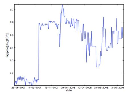
Figure 1. Log price of the Kalev stock [3]

Kobayashi [6] introduced the duality theorem between time-changed SDEs and the corresponding non-time-changed SDEs, and established the Itô formula for time-changed SDEs. Soon after Kobayashi’s fruitful results, Wu [15] established the stochastic and moment stabilities of the solution to the SDEs driven by time-changed Brownian motion

(1.3) $$dX(t)=k(t,E_{t},X(t-))+f(t,E_{t},X(t-))dt+g(t,E_{t},X(t-))dB_{E_{t}},\ t\geq 0,$$

with $X(0)=x_{0}$, where $E_{t}$ is specified as the inverse of an $\alpha$-stable subordinator, $\alpha\in(0,1)$. In our recent paper [12], we focus on the following time-changed SDE

(1.4) $$dX(t) =f(t,E_{t},X(t-))dt+k(t,E_{t},X(t-))dE_{t}+g(t,E_{t},X(t-))dB_{E_{t}}$$

$$+\int_{|y|<c}h(t,E_{t},X(t-),y)\tilde{N}(dE_{t},dy),$$

with $X(t_{0})=x_{0}$, where $E_{t}$ is the inverse of a strictly increasing subordinator, and discuss stability of its solution in probability and moment senses, including stochastical stability, stochastical asymptotic stability, global stochastic asymptotic stability, $p$th moment exponential stability and $p$th moment asymptotic stability.

In this paper, we analyze the path stabilities of the solution to (1.4) and the following stochastic differential equation with linear jumps

(1.5) $$dX(t) =f(t,E_{t},X(t-))dt+k(t,E_{t},X(t-))dE_{t}+g(t,E_{t},X(t-))dB_{E_{t}}$$

$$+\int_{|y|<c}h(y)X(t-)\tilde{N}(dE_{t},dy)+\int_{|y|\geq c}H(y)X(t-)N(dE_{t},dy).$$

with $X(t_{0})=x_{0}$, where $E_{t}$ is the inverse of a ”mixed” subordinator.

In the remaining parts of this paper, further needed concepts and related background will be given in section 2. In section 3, the conditions for the solution to our target time-changed SDEs to be almost sure exponential path stability and almost sure path stability will be given. Connections between stability of the solution to time-changed SDE and that of the corresponding non-time-changed SDE will be disclosed and some examples will be provided.

2. Preliminaires

Let $(\Omega,\mathcal{F},(\mathcal{F}_{t}),P)$ be a filtered probability space satisfying usual hypotheses of completeness and right continuity. Assume that $\mathcal{F}_{t}$-adapted Poisson random measure $N$ on $\mathbb{R}_{+}\times(\mathbb{R}-\{0\})$ is independent of the drift and the standard Brownian motion, define its compensator $\tilde{N}(dt,dy)=N(dt,dy)-\nu(dy)dt$, where $\nu$ is a Lévy measure satisfying $\int_{\mathbb{R}-\{0\}}(|y|^{2}\land 1)\nu(dy)<\infty$.

Let $\{D(t),t\geq 0\}$ be a RCLL increasing Lévy process that is called subordinator starting from 0 with Laplace transform

(2.1) $$\mathbbm{E}e^{-sD(t)}=e^{-t\psi(s)},$$

where Laplace exponent $\psi(s)=\int_{0}^{\infty}(1-e^{-sx})\nu(dx)$.

Define its inverse

(2.2) $$E_{t}:=\inf\{\tau>0:D(\tau)>t\}.$$

The concept of regular variation is needed to introduce the mixed stable subordinator. A measurable function R is regularly varying at infinity with exponent $\gamma\in\mathbb{R}$, denoted by $R\in RV_{\infty}(\gamma)$, if R is eventually positive and $R(ct)/R(t)\rightarrow c^{\gamma}$ as $t\rightarrow\infty$, for any $c>0$. Similarly, a measurable function R is regularly varying at zero with exponent $\gamma\in\mathbb{R}$, denoted by $R\in RV_{0}(\gamma)$, if R is positive in some neighborhood of zero and $R(ct)/R(t)\rightarrow c\gamma$ as $t\rightarrow 0$, for any $c>0$.

Given a measurable function $p:(0,1)\rightarrow\mathbb{R}_{+}$ such that $p\in RV_{0}(\gamma-1)$ for some $\gamma>0$, let $L(u)=C\int_{0}^{1}u^{-\alpha}p(\alpha)d\alpha$ and $C^{-1}=\int_{0}^{1}p(\alpha)d\alpha$. Without loss of generality, let $C=1$, then $p$ is a probability density of Lévy measure of the $\alpha$-stable subordinators. Let $\{D(t)\}_{t\geq 0}$ be a subordinator such that $D(1)$ has Lévy-Khinchin representation $[0,0,\phi]$ and the Lévy measure $\phi$ is defined as $\phi(u,\infty)=L(u)$, then $\{D(t)\}_{t\geq 0}$ is the so called ”mixed” stable subordinator. In this case the Laplace exponent is given by

(2.3) $$\psi(s)=\int_{0}^{1}\Gamma(1-\beta)s^{\beta}p(\beta)d\beta$$

By Theorem 3.9 in [10], there exists a function $L\in RV_{\infty}(0)$ such that

(2.4) $$\mathbb{E}[E(t)]\sim(\log t)^{\gamma}L(\log t)^{-1}\ \ as\ t\rightarrow\infty.$$

We require $f,k,g,h,H$ in (1.4) and (1.5) to be real-valued functions and satisfy the following Lipschitz condition in Assumption 2.1, growth condition in Assumption 2.2 and Assumption 2.3. Under these assumptions, by Lemma 4.1 in [6], both of the equations (1.4) and (1.5) have unique $\mathcal{G}_{t}=\mathcal{F}_{E_{t}}$-adapted solution processes $X(t)$.

Assumption 2.1.

(Lipschitz condition) There exists a positive constant $K_{1}$ such that

(2.5) $$\Big{|}f(t_{1},t_{2},x)-f(t_{1},t_{2},y)\Big{|}^{2}+\Big{|}k(t_{1},t_{2},x)-k(t_{1},t_{2},y)\Big{|}^{2}+\Big{|}g(t_{1},t_{2},x)-g(t_{1},t_{2},y)\Big{|}^{2}$$

$$+\int_{|z|<c}\Big{|}h(t_{1},t_{2},x,z)-h(t_{1},t_{2},y,z)\Big{|}^{2}\nu(dz)\leq K_{1}|x-y|^{2},$$

for all $t_{1},t_{2}\in\mathbb{R}_{+}$ and $x,y\in\mathbb{R}$.

Assumption 2.2.

(Growth condition) There exists a positive constant $K_{2}$ such that, for all $t_{1},t_{2}\in\mathbb{R}_{+}$ and $x\in\mathbb{R}$,

(2.6) $$|f(t_{1},t_{2},x)|^{2}+|k(t_{1},t_{2},x)|^{2}+|g(t_{1},t_{2},x)|^{2}+\int_{|y|<c}|h(t_{1},t_{2},x,y)|^{2}\nu(dy)\leq K_{2}(1+|x|^{2}).$$

Assumption 2.3.

If $X(t)$ is right continuous with left limits (rcll) and a $\mathcal{G}_{t}$-adapted process, then

(2.7) $$f(t,E_{t},X(t)),k(t,E_{t},X(t)),g(t,E_{t},X(t)),h(t,E_{t},X(t),y)\in\mathcal{L}(\mathcal{G}_{t}),$$

where $\mathcal{L}(\mathcal{G}_{t})$ denotes the class of rcll and $\mathcal{G}_{t}$-adapted processes.

Note that the Stochastic differential equation (1.4) involves only Lévy process with small jumps and general scalars for the drift and the standard Brownian motion and Poisson jump; while the linear stochastic differential equation (1.5) contains both small and large Poisson jumps with linear scalars. Next, we define two different types of stability.

Definition 2.4.

(Definition 3.1 in [9]) The trivial solution of the time-changed SDE (1.4) is said to be almost surely exponentially path stable if

(2.8) $$\limsup_{t\rightarrow\infty}\frac{1}{t}\log|X(t;t_{0},x_{0})|<0\ \ a.s.$$

for all $x_{0}\in R$.

Definition 2.5.

The trivial solution of the time-changed SDE (1.4) is said to be almost surely path stable if there exists a function $\nu(t):[0,\infty)\rightarrow[0,\infty)$ such that

(2.9) $$\lim_{t\rightarrow\infty}\nu(t)=\infty,$$

and

(2.10) $$\limsup_{t\rightarrow\infty}\frac{1}{\nu(t)}\log|X(t;t_{0},x_{0})|<0\ \ a.s.$$

for all $x_{0}\in R$.

The Itô formula is heavily used in our proofs. We derive the following Itô formula for time-changed Lévy noise and will utilize it frequently in the remaining sections.

Lemma 2.6.

(Itô formula for time-changed Lévy noise) Let $D(t)$ be a rcll subordinator and its inverse process $E_{t}:=\inf\{\tau>0:D(\tau)>t\}$. Define a filtration $\{\mathcal{G}_{t}\}_{t\geq 0}$ by $\mathcal{G}_{t}=\mathcal{F}_{E_{t}}$. Let $X$ be a process satisfying the following:

(2.11) $$X(t) =x_{0}+\int_{t_{0}}^{t}f(s,E_{s},X(s-))ds+\int_{t_{0}}^{t}k(s,E_{s},X(s-))dE_{s}+\int_{t_{0}}^{t}g(s,E_{s},X(s-))dB_{E_{s}}$$

$$+\int_{t_{0}}^{t}\int_{|y|<c}h(s,E_{s},X(s-),y)\tilde{N}(dE_{s},dy)+\int_{t_{0}}^{t}\int_{|y|\geq c}H(s,E_{s},X(s-),y)N(dE_{s},dy),$$

where $f,k,g,h,H$ are measurable functions such that all integrals are defined, $c$ is a positive constant.

Then, for all $F:\mathbb{R}_{+}\times\mathbb{R}_{+}\times\mathbb{R}\rightarrow\mathbb{R}$ in $C^{1,1,2}(\mathbb{R}_{+}\times\mathbb{R}_{+}\times\mathbb{R},\mathbb{R})$, we have with probability one,

(2.12) $$F(t,E_{t}, X(t))-F({t_{0}},E_{t_{0}},x_{0})=\int_{t_{0}}^{t}L_{1}F(s,E_{s},X(s-))ds+\int_{t_{0}}^{t}L_{2}F(s,E_{s},X(s-))dE_{s}$$

$$+\int_{t_{0}}^{t}\int_{|y|<c}\Big{[}F(s,E_{s},X(s-)+h(s,E_{s},X(s-),y))-F(s,E_{s},X(s-))\Big{]}\tilde{N}(dE_{s},dy)$$

$$+\int_{t_{0}}^{t}\int_{|y|\geq c}\Big{[}F(s,E_{s},X(s-)+H(s,E_{s},X(s-),y))-F(s,E_{s},X(s-))\Big{]}N(dE_{s},dy)$$

$$+\int_{t_{0}}^{t}F_{x}(s,E_{s},X(s-))g(s,E_{s},X(s-))dB_{E_{s}},$$

where

(2.13) $$L_{1}F(t_{1}, t_{2},x)=F_{t_{1}}(t_{1},t_{2},x)+F_{x}(t_{1},t_{2},x)f(t_{1},t_{2},x),$$

$$L_{2}F(t_{1}, t_{2},x)=F_{t_{2}}(t_{1},t_{2},x)+F_{x}(t_{1},t_{2},x)k(t_{1},t_{2},x)+\frac{1}{2}g^{2}(t_{1},t_{2},x)F_{xx}(t_{1},t_{2},x)$$

$$+ \int_{|y|<c}\Big{[}F(t_{1},t_{2},x+h(t_{1},t_{2},x,y))-F(t_{1},t_{2},x)-F_{x}(t_{1},t_{2},x)h(t_{1},t_{2},x,y)\Big{]}\nu(dy).$$

Note that the proof of the Itô formula for time-changed Lévy noise follows by similar ideas as in the proof of Lemma 3.1 in [12], thus the details are omitted. To perform future analysis, we need some conditions under which the solutions of (1.4) can not reach the origin after certain time $t_{0}$ given that $X(t_{0})\neq 0$.

Assumption 2.7.

For any $\theta>0$ there exists $K_{\theta}>0$, such that

(2.14) $$|k(x)|+|g(x)|+2\int_{|y|<c}\frac{|h(x,y)|(|x|+|h(x,y)|)}{|x+h(x,y)|}\nu(dy)\leq K_{\theta}|x|$$

and

(2.15) $$|f(x)|\leq K_{\theta}|x|^{2}\ ,for\ 0<|x|\leq\theta.$$

Lemma 2.8.

Given that the assumption (2.7) holds, the solution of (1.4) satisfies

(2.16) $$P(X(t)\neq 0\ for\ all\ t\geq t_{0})=1,$$

if $x_{0}\neq 0$.

Proof.

We follow the idea in the proof of Lemma 3.4.4 in [14] and prove this result by contradiction. Suppose that (2.16) is not true, that is, there exists initial condition $x_{0}\neq 0$ and stopping time $\tau$ with $P(\tau<\infty)>0$ where

(2.17) $$\tau=\inf\{t\geq t_{0}:|X(t)|=0\}.$$

Since the paths of $X(t)$ are right continuous with left limit (rcll), there exist $T>0$ and $\theta>1$ sufficiently large such that $P(B)>0$, where

(2.18) $$B=\{w\in\Omega:\tau(w)\leq T\ and\ |X(t)(w)|\leq\theta-1\ for\ all\ t_{0}<t<\tau(w)\}.$$

Next, define another stopping time

(2.19) $$\tau_{\epsilon}=\inf\{t\geq t_{0}:|X(t)|\leq\epsilon\ or\ |X(t)|\geq\theta\}$$

for each $0<\epsilon<|X(t_{0})|$.

Let $\lambda=2K_{\theta}+\frac{K_{\theta}^{2}}{2}$ be a constant and define $Z(t)=e^{-\lambda E_{t}}|X(t)|^{-1}$. Since $Z(t)=e^{-\lambda E_{t}}|X(t)|^{-1}$ is $C^{1,1,2}$ except at $X(t)=0$, and by definition of $\tau_{\epsilon}$, $X(t)$ will not reach 0 for $t_{0}\leq t\leq\tau_{\epsilon}\land T$, so Itô formula can be applied to $e^{-\lambda(E_{\tau_{\epsilon}\land T})}|X(\tau_{\epsilon}\land T)|^{-1}$.

By (2.14) and (2.15),

(2.20) $$e^{-\lambda(E_{\tau_{\epsilon}\land T})}|X(\tau_{\epsilon}\land T)|^{-1}-|x_{0}|^{-1}$$

$$= \int_{t_{0}}^{\tau_{\epsilon}\land T}e^{-\lambda E_{s}}[-\frac{X(s-)f(X(s-))}{|X(s-)|^{3}}]ds+\frac{1}{2}\int_{t_{0}}^{\tau_{\epsilon}\land T}e^{-\lambda E_{s}}\frac{g(X(s-))^{2}}{|X(s-)|^{3}}dE_{s}$$

$$+\int_{t_{0}}^{\tau_{\epsilon}\land T}e^{-\lambda E_{s}}\frac{-1}{|X(s-)|^{2}}\Big{[}\lambda|X(s-)|dE_{s}+k(X(s-))dE_{s}+g(X(s-))dB_{E_{s}}\Big{]}$$

$$+\int_{t_{0}}^{\tau_{\epsilon}\land T}\int_{|y|<c}e^{-\lambda E_{s}}\Big{[}\frac{1}{|X(s-)+h(X(s-),y)|}-\frac{1}{|X(s-)|}\Big{]}\tilde{N}(dE_{s},dy)$$

$$+\int_{t_{0}}^{\tau_{\epsilon}\land T}\int_{|y|<c}e^{-\lambda E_{s}}\Big{[}\frac{1}{|X(s-)+h(X(s-),y)|}-\frac{1}{|X(s-)|}+\frac{X(s-)h(X(s-),y)}{|X(s-)|^{3}}\Big{]}\nu(dy)dE_{s}$$

$$\leq \int_{t_{0}}^{\tau_{\epsilon}\land T}e^{-\lambda E_{s}}K_{\theta}ds+\int_{t_{0}}^{\tau_{\epsilon}\land T}e^{-\lambda E_{s}}\frac{-g(X(s-))X(s-)}{|X(s-)|^{3}}dB_{E_{s}}$$

$$+\int_{t_{0}}^{\tau_{\epsilon}\land T}e^{-\lambda E_{s}}\Bigg{[}\frac{-\lambda}{|X(s-)|}+\frac{-k(X(s-))X(s-)}{|X(s-)|^{3}}+\frac{g(X(s-))^{2}}{2|X(s-)|^{3}}$$

$$+\int_{|y|<c}\Big{[}\frac{1}{|X(s-)+h(X(s-),y)|}-\frac{1}{|X(s-)|}+\frac{X(s-)h(X(s-),y)}{|X(s-)|^{3}}\Big{]}\nu(dy)\Bigg{]}dE_{s}$$

$$+\int_{t_{0}}^{\tau_{\epsilon}\land T}\int_{|y|<c}e^{-\lambda s}\Big{[}\frac{1}{|X(s-)+h(X(s-),y)|}-\frac{1}{|X(s-)|}\Big{]}\tilde{N}(dE_{s},dy)$$

$$\leq K_{\theta}\tau_{\epsilon}\land T+\int_{t_{0}}^{\tau_{\epsilon}\land T}e^{-\lambda E_{s}}\Big{[}\frac{-\lambda}{|X(s-)|}+\frac{2K_{\theta}+\frac{K_{\theta}^{2}}{2}}{|X(s-)|}\Big{]}dE_{s}+\int_{t_{0}}^{\tau_{\epsilon}\land T}e^{-\lambda E_{s}}\frac{-g(X(s-))X(s-)}{|X(s-)|^{3}}dB_{E_{s}}$$

$$+\int_{t_{0}}^{\tau_{\epsilon}\land T}\int_{|y|<c}e^{-\lambda E_{s}}\Big{[}\frac{1}{|X(s-)+h(X(s-),y)|}-\frac{1}{|X(s-)|}\Big{]}\tilde{N}(dE_{s},dy)$$

$$\leq K_{\theta}T+\int_{t_{0}}^{\tau_{\epsilon}\land T}e^{-\lambda E_{s}}\frac{-g(X(s-))X(s-)}{|X(s-)|^{3}}dB_{E_{s}}$$

$$+\int_{t_{0}}^{\tau_{\epsilon}\land T}\int_{|y|<c}e^{-\lambda E_{s}}\Big{[}\frac{1}{|X(s-)+h(X(s-),y)|}-\frac{1}{|X(s-)|}\Big{]}\tilde{N}(dE_{s},dy)$$

The penultimate inequality is derived from lemma 3.4.2 on page 54 of [14], which states that $\frac{1}{|x+y|}-\frac{1}{|x|}+\frac{xy}{|x|^{3}}\leq\frac{2|y|}{|x|^{2}}\frac{(|y|+|x|)}{|x+y|}$ for $x,y,x+y\neq 0$, thus

(2.21) $$\int_{|y|<c}\Big{[}\frac{1}{|X(s-)+h(X(s-),y)|}-\frac{1}{|X(s-)|}+\frac{X(s-)h(X(s-),y)}{|X(s-)|^{3}}\Big{]}\nu(dy)$$

$$\leq \int_{|y|<c}\frac{2|h(X(s-),y)|}{|X(s-)|^{2}}\Big{[}\frac{|h(X(s-),y)|+|X(s-)|}{|h(X(s-),y)+X(s-)|}\Big{]}\nu(dy)$$

$$= \frac{1}{|X(s-)|^{2}}\int_{|y|<c}\frac{2|h(X(s-),y)|(|h(X(s-),y)|+|X(s-)|)}{|h(X(s-),y)+X(s-)|}\nu(dy)$$

$$\leq \frac{K_{\theta}|X(s-)|}{|X(s-)|^{2}}=\frac{K_{\theta}}{|X(s-)|}.$$

Observe that the last two terms in the last line of the inequality (2.20) are martingales. Then by taking expectations of both sides, we derive that

(2.22) $$\mathbb{E}\Big{[}e^{-\lambda(E_{\tau_{\epsilon}\land T})}|X(t)|^{-1}\Big{]}\leq|x_{0}|^{-1}+K_{\theta}T.$$

If $w\in B$, then $\tau_{\epsilon}(w)\leq T$ and $|X(\tau_{\epsilon}(w))|\leq\epsilon$, then

(2.23) $$\mathbb{E}\Big{[}e^{-\lambda E_{\tau_{\epsilon}\land T}}\epsilon^{-1}\mathbbm{1}_{B}\big{]}\leq\mathbb{E}\Big{[}e^{-\lambda E_{\tau_{\epsilon}\land T}}|X(\tau_{\epsilon}(w))|^{-1}\mathbbm{1}_{B}\big{]}\leq\mathbb{E}\Big{[}e^{-\lambda E_{\tau_{\epsilon}\land T}}|X(\tau_{\epsilon}(w))|^{-1}\big{]}\leq|x_{0}|^{-1}+K_{\theta}T.$$

Recall the reverse Hölder’s inequality: for all $p>1$

$$E(|XY|)\geq(E|X|^{1/p})^{p}(E(|Y|^{-1/(p-1)}))^{-(p-1)}.$$

We use the reverse Hölder’s inequality with $p=2$, $X=\mathbbm{1}_{B}$ and $Y=e^{-\lambda E_{\tau_{\epsilon}\land T}}$. Since $X^{1/2}=X$, this gives

$$[\mathbb{P}(B)]^{2}\Bigg{[}E(e^{\lambda E_{\tau_{\epsilon}\land T}})\Bigg{]}^{-1}\leq\mathbb{E}\Big{[}e^{-\lambda E_{\tau_{\epsilon}\land T}}\mathbbm{1}_{B}\big{]}\leq\epsilon(|x_{0}|^{-1}+K_{\theta}T),\ for\ all\ \epsilon\geq 0$$

Since the inverse subordinator has finite exponential moment, $E(e^{(\lambda E_{\tau_{\epsilon}\land T})})$ is finite for any fixed time $T$, see Lemma 8 in [5]. Then, letting $\epsilon\rightarrow 0$, we obtain $P(B)=0$, which contradicts the assumption, thus the desired result is correct. ∎

Remark 2.9.

When the Laplace exponent of the subordinator is given by (2.3), an alternative method to show that the expectation $E(e^{(\lambda E_{\tau_{\epsilon}\land T}}))$ is finite is to use the moments of $E_{t}$. Since $\{E_{t},t\geq 0\}$ is nonnegative and nondecreasing, we have $\tau_{\epsilon}\land T\leq T$. Because $\lambda>0$, $e^{x}$ is a strictly positive and increasing function, $E(e^{\lambda E_{\tau_{\epsilon}\land T}})\leq E(e^{\lambda E_{T}})$. Thus, it is sufficient to show that $E(e^{\lambda E_{T}})$ is finite. By Theorem 3.9 in [10], there exists a function $L\in RV_{\infty}(0)$ such that for any $n>0$,$\gamma>0$ and sufficiently large $t$,

(2.24) $$\mathbb{E}[E_{t}^{n}]\sim(\log t)^{\gamma n}L(\log t)^{-n}.$$

By Taylor expansion and Fubini theorem,

(2.25) $$\mathbb{E}[\exp(\lambda E_{t})] =\mathbb{E}[\sum_{n=0}^{\infty}\frac{\lambda^{n}{E_{t}}^{n}}{n!}]=\sum_{n=0}^{\infty}\frac{\lambda^{n}\mathbb{E}[{E_{t}}^{n}]}{n!}\sim\sum_{n=0}^{\infty}\frac{\lambda^{n}(\log t)^{\gamma n}L(\log t)^{-n}}{n!}$$

$$=\sum_{n=0}^{\infty}\frac{(\lambda(\log t)^{\gamma}L(\log t)^{-1})^{n}}{n!}=\exp(\lambda(\log t)^{\gamma}L(\log t)^{-1}).$$

Hence, for fixed large $t$, $\mathbb{E}[\exp(\lambda E_{t})]\sim\exp(\lambda(\log t)^{\gamma}L(\log t)^{-1})$ is finite.

A similar method applies when the Laplace exponent of the subordinator $D(t)$ is given by

(2.26) $$\psi(s)=\sum_{i=1}^{k}c_{i}s^{\beta_{i}},$$

where $\sum_{i=1}^{k}c_{i}=1$ and $0<\beta_{1}<\beta_{2}<...<\beta_{k}<1$. Then the Laplace transform of the $n$-th moment of $E_{t}$ is $\mathcal{L}(\mathbb{E}(E_{t}^{n}))(s)=\frac{n!}{s(\sum_{i=1}^{k}c_{i}s^{\beta_{i}})^{n}}$; see Lemma 8 in [5]. Using the Karamata Tauberian Theorem (see [2], Theorem 1 and Lemma on pp. 443-446) we can deduce that for large $t$, $\mathbb{E}(E_{t}^{n})\approx C_{n}t^{n\beta_{1}}$

Lemma 2.10.

(Time-Changed Exponential Martingale Inequality) Let $D(t)$ be a rcll subordinator and its inverse process $E_{t}:=\inf\{\tau>0:D(\tau)>t\}$. Let T, $\lambda,\kappa$ be any positive numbers, $B_{c}=\{y\in\mathbb{R}:|y|<c\}$. Assume $g:\mathbb{R^{+}}\rightarrow\mathbb{R}$ and $h:\mathbb{R}^{+}\times B_{c}\rightarrow\mathbb{R}$ satisfy $\mathbb{E}[\int_{0}^{T}|g(t)|^{2}dE_{t}]<\infty$ and $\mathbb{E}[\int_{0}^{T}\int_{|y|<c}|h(t,y)|^{2}\nu(dy)dE_{t}]<\infty$, then

(2.27) $$P\Big{[}\sup_{0\leq t\leq T}\Big{\{}\int_{0}^{t}g(s)dB_{E_{s}}-\frac{\lambda}{2}\int_{0}^{t}|g(s)|^{2}dE_{s}+\int_{0}^{t}\int_{|y|<c}h(s,y)\tilde{N}(dE_{s},dy)$$

$$-\frac{1}{\lambda}\int_{0}^{t}\int_{|y|<c}\Big{[}\exp(\lambda h(s,y))-1-\lambda h(s,y)\Big{]}\nu(dy)dE_{s}\Big{\}}>\kappa\Big{]}\leq\exp(-\lambda\kappa)$$

Proof.

Define a sequence of stopping times $(\tau_{n},n\geq 1)$ as below

(2.28) $$\tau_{n}= \inf\Big{\{}t\geq 0:\bigg{|}\int_{0}^{t}g(s)dB_{E_{s}}\bigg{|}+\frac{\lambda}{2}\int_{0}^{t}|g(s)|^{2}dE_{s}+\bigg{|}\int_{0}^{t}\int_{|y|<c}h(s,y)\tilde{N}(dE_{s},dy)\bigg{|}$$

$$+\frac{1}{\lambda}\bigg{|}\int_{0}^{t}\int_{|y|<c}\Big{[}\exp(\lambda h(s,y))-1-\lambda h(s,y)\Big{]}\nu(dy)dE_{s}\bigg{|}\geq n\Big{\}},\ for\ n\geq 1.$$

Note that $\tau_{n}\rightarrow\infty$ as $n\rightarrow\infty$ a.s.

Define the following Itô process

(2.29) $$X_{n}(t)= \lambda\int_{0}^{t}g(s)\mathbbm{1}_{[0,\tau_{n}]}(s)dB_{E_{s}}-\frac{\lambda^{2}}{2}\int_{0}^{t}|g(s)|^{2}\mathbbm{1}_{[0,\tau_{n}]}(s)dE_{s}$$

$$+\lambda\int_{0}^{t}\int_{|y|<c}h(s,y)\mathbbm{1}_{[0,\tau_{n}]}(s)\tilde{N}(dE_{s},dy)$$

$$-\int_{0}^{t}\int_{|y|<c}\Big{[}\exp(\lambda h(s,y))-1-\lambda h(s,y)\Big{]}\mathbbm{1}_{[0,\tau_{n}]}(s)\nu(dy)dE_{s},$$

with $X_{n}(0)=0$ for all $n\geq 0$. Then for all $0\leq t\leq T$

(2.30) $$|X_{n} (t)|\leq\lambda\Big{|}\int_{0}^{t}g(s)\mathbbm{1}_{[0,\tau_{n}]}(s)dB_{E_{s}}\Big{|}+\Big{|}\lambda\int_{0}^{t}\int_{|y|<c}h(s,y)\mathbbm{1}_{[0,\tau_{n}]}(s)\tilde{N}(dE_{s},dy)\Big{|}$$

$$+\frac{\lambda^{2}}{2}\int_{0}^{t}|g(s)|^{2}\mathbbm{1}_{[0,\tau_{n}]}(s)dE_{s}+\Big{|}\int_{0}^{t}\int_{|y|<c}\Big{[}\exp(\lambda h(s,y))-1-\lambda h(s,y)\Big{]}\mathbbm{1}_{[0,\tau_{n}]}(s)\nu(dy)dE_{s}\Big{|}$$

$$\leq\lambda n.$$

Let $Z(t)=\exp(X_{n}(t))$, by the time-changed Itô’s formula (2.12),

(2.31) $$\exp (X_{n}(t))-\exp(x_{0})$$

$$= \int_{0}^{t}\exp(X_{n}(s))\Big{[}-\frac{\lambda^{2}}{2}|g(s)|^{2}\mathbbm{1}_{[0,\tau_{n}]}(s)-\int_{|y|<c}\big{[}\exp(\lambda h(s,y))-1-\lambda h(s,y)\big{]}\mathbbm{1}_{[0,\tau_{n}]}(s)\nu(dy)$$

$$+\int_{|y|<c}\big{[}\exp(\lambda h(s,y))-1-\lambda h(s,y)\big{]}\mathbbm{1}_{[0,\tau_{n}]}(s)\nu(dy)+\frac{\lambda^{2}}{2}|g(s)|^{2}\mathbbm{1}_{[0,\tau_{n}]}(s)\Big{]}dE_{s}$$

$$+\int_{0}^{t}\int_{|y|<c}\big{[}\exp(X_{n}(s)+\lambda h(s,y))-\exp(X_{n}(s))\big{]}\mathbbm{1}_{[0,\tau_{n}]}(s)\tilde{N}(dE_{s},dy)$$

$$+\lambda\int_{0}^{t}\exp(X_{n}(s))g(s)\mathbbm{1}_{[0,\tau_{n}]}(s)dB_{E_{s}}$$

$$= \int_{0}^{t}\int_{|y|<c}\big{[}\exp(X_{n}(s)+\lambda h(s,y))-\exp(X_{n}(s))\big{]}\mathbbm{1}_{[0,\tau_{n}]}(s)\tilde{N}(dE_{s},dy)$$

$$+\lambda\int_{0}^{t}\exp(X_{n}(s))g(s)\mathbbm{1}_{[0,\tau_{n}]}(s)dB_{E_{s}},$$

thus $\{\exp(X_{n}(t)),0\leq t\leq T\}$ is a local martingale. Since we have

(2.32) $$\sup_{t\in[0,T]}\exp(X_{n}(t))\leq\exp(\lambda n)\ \ a.s.$$

there exists a sequence of stopping times $(T_{m},m\in\mathbbm{N})$ with $(T_{m}\rightarrow\infty)(a.s.)$ as $n\rightarrow\infty$ such that for all $0\leq s\leq t\leq T$

(2.33) $$\mathbbm{E}[\exp(X_{n}(t\wedge T_{m}))|\mathcal{F}_{s}]=\exp(X_{n}(s\wedge T_{m}))\leq\exp(\lambda n)\ \ a.s.$$

By Dominated Convergence Theorem, we have

(2.34) $$\mathbb{E}[\exp(X_{n}(t))|\mathcal{F}_{s}]=\lim_{m\rightarrow\infty}\mathbbm{E}[\exp(X_{n}(t\wedge T_{m}))|\mathcal{F}_{s}]=\lim_{m\rightarrow\infty}\exp(X_{n}(s\wedge T_{m}))=\exp(X_{n}(s)),$$

that is, $Z(t)=\exp(X_{n}(t))$ is a martingale for all $0\leq t\leq T$ with $\mathbbm{E}[\exp(X_{n}(t))]=1$.

Apply Doob’s martingale inequality

(2.35) $$\mathbb{P}\Big{[}\sup_{0\leq t\leq T}\exp(X_{n}(t))\geq\exp(\lambda\kappa)\Big{]}\leq\exp(-\lambda\kappa)\mathbbm{E}[\exp(X_{n}(T))]=\exp(-\lambda\kappa),$$

equivalently,

(2.36) $$\mathbb{P}\Big{[}\sup_{0\leq t\leq T}\frac{X_{n}(t)}{\lambda}\geq\kappa\Big{]}\leq\exp(-\lambda\kappa),$$

writing $\exp(X_{n}(t))$ explicitly, we have

(2.37) $$\mathbb{P}\Big{[}\sup_{0\leq t\leq T}\Big{\{} \int_{0}^{t}g(s)\mathbbm{1}_{[0,\tau_{n}]}(s)dB_{E_{s}}-\frac{\lambda}{2}\int_{0}^{t}|g(s)|^{2}\mathbbm{1}_{[0,\tau_{n}]}(s)dE_{s}$$

$$+\int_{0}^{t}\int_{|y|<c}h(s,y)\mathbbm{1}_{[0,\tau_{n}]}(s)\tilde{N}(dE_{s},dy)$$

$$-\frac{1}{\lambda}\int_{0}^{t}\int_{|y|<c}\Big{[}\exp(\lambda h(s,y))-1-\lambda h(s,y)\Big{]}\mathbbm{1}_{[0,\tau_{n}]}(s)\nu(dy)dE_{s}\Big{\}}\geq\kappa\Big{]}\leq\exp(-\lambda\kappa)$$

Define

(2.38) $$A_{n}=\Big{\{}w\in\Omega:\sup_{0\leq t\leq T}\Big{\{} \int_{0}^{t}g(s)\mathbbm{1}_{[0,\tau_{n}]}(s)dB_{E_{s}}-\frac{\lambda}{2}\int_{0}^{t}|g(s)|^{2}\mathbbm{1}_{[0,\tau_{n}]}(s)dE_{s}$$

$$+\int_{0}^{t}\int_{|y|<c}h(s,y)\mathbbm{1}_{[0,\tau_{n}]}(s)\tilde{N}(dE_{s},dy)$$

$$-\frac{1}{\lambda}\int_{0}^{t}\int_{|y|<c}\Big{[}\exp(\lambda h(s,y))-1-\lambda h(s,y)\Big{]}\mathbbm{1}_{[0,\tau_{n}]}(s)\nu(dy)dE_{s}\Big{\}}\geq\kappa\Big{\}},$$

then $\mathbb{P}(A_{n})\leq\exp(-\lambda\kappa)$.

Since

(2.39) $$\mathbb{P}[\liminf_{n\rightarrow\infty}A_{n}]\leq\liminf_{n\rightarrow\infty}\mathbb{P}(A_{n})\leq\limsup_{n\rightarrow\infty}\mathbb{P}(A_{n})\leq\mathbb{P}[\limsup_{n\rightarrow\infty}A_{n}]$$

and

(2.40) $$\limsup_{n\rightarrow\infty}\mathbb{P}(A_{n})\leq\exp(-\lambda\kappa),$$

also

(2.41) $$\limsup_{n\rightarrow\infty}A_{n}=\liminf_{n\rightarrow\infty}A_{n}=A,$$

where

(2.42) $$A=\Big{\{}w\in\Omega:\sup_{0\leq t\leq T}\Big{\{} \int_{0}^{t}g(s)dB_{E_{s}}-\frac{\lambda}{2}\int_{0}^{t}|g(s)|^{2}dE_{s}+\int_{0}^{t}\int_{|y|<c}h(s,y)\tilde{N}(dE_{s},dy)$$

$$-\frac{1}{\lambda}\int_{0}^{t}\int_{|y|<c}\Big{[}\exp(\lambda h(s,y))-1-\lambda h(s,y)\Big{]}\nu(dy)dE_{s}\Big{\}}\geq\kappa\Big{\}},$$

thus

(2.43) $$\mathbb{P}(A)=\mathbb{P}[\liminf_{n\rightarrow\infty}A_{n}]\leq\limsup_{n\rightarrow\infty}P(A_{n})\leq\limsup_{n\rightarrow\infty}\exp(-\lambda\kappa)=\exp(-\lambda\kappa).$$

∎

The next result can be considered as a strong law of large numbers for the inverse subordinator.

Lemma 2.11.

Let $\{E_{t}\}_{t\geq 0}$ be the inverse of the mixed stable subordinator $D(t)$ with laplace exponent given in (2.3) as defined in (2.2), then

(2.44) $$\lim_{t\rightarrow\infty}\frac{E_{t}}{t}=0,\ a.s.$$

Proof.

Fix $\epsilon>0$ and define

(2.45) $$A_{n}=\Big{\{}\sup_{2^{n}<t<2^{n+1}}\Big{|}\frac{E_{t}}{t}\Big{|}>\epsilon\Big{\}},$$

then, by Markov’s inequality and equation (2.4), as $n\rightarrow\infty$, for some $\gamma>0$,

(2.46) $$\epsilon\mathbb{P}(A_{n}) \leq\mathbb{E}\Big{[}\sup_{2^{n}<t<2^{n+1}}\Big{|}\frac{E_{t}}{t}\Big{|}\Big{]}\leq\mathbb{E}\Big{[}\Big{|}\frac{E_{2^{n+1}}}{2^{n}}\Big{|}\Big{]}\sim\frac{[\log(2^{n+1})]^{\gamma}L(\log(2^{n+1}))^{-1}}{2^{n}}$$

$$=\frac{(n+1)^{\gamma}(\log 2)^{\gamma}L(\log(2^{n+1}))^{-1}}{2^{n}}\sim\frac{C(n+1)^{\gamma}}{2^{n}}.$$

By the ratio test, $\sum_{n=1}^{\infty}\mathbb{P}(A_{n})<\infty$. Applying Borel-Cantelli lemma, we have

(2.47) $$\lim_{t\rightarrow\infty}\frac{E_{t}}{t}=0,\ a.s.$$

∎

Remark 2.12.

Lemma 2.11 can also be proved for discrete case with the help of Laplace transform. Let $E_{t}$ be an inverse of the subordinator with Laplace exponent $\psi(s)=\sum_{i=1}^{k}c_{i}s^{\beta_{i}}$, where $\sum_{i=1}^{k}c_{i}=1$ and $0<\beta_{1}<\beta_{2}<...<\beta_{k}<1$. Then the Laplace transform of the $nth$ moment of $E_{t}$ is $\mathcal{L}(\mathbb{E}(E_{t}^{n}))(s)=\frac{n!}{s(\sum_{i=1}^{k}c_{i}s^{\beta_{i}})^{n}}$.

By a Karamata Tauberian theorem (see [2], Theorem 1 and Lemma on pp. 443-446), since $\mathcal{L}(\mathbb{E}(E_{t}))(s)\sim cs^{-(1+\beta_{1})}$ as $s\to 0$ then $\mathbb{E}(E_{t})\sim Ct^{\beta_{1}}$ as $t\rightarrow\infty$. Utilizing this result, $\epsilon\mathbb{P}(A_{n})\leq\mathbb{E}\Big{[}\Big{|}\frac{E_{2^{n+1}}}{2^{n}}\Big{|}\Big{]}\sim\frac{(2^{n+1})^{\beta_{1}}}{2^{n}}=2^{\beta_{1}}2^{-(1-\beta_{1})n}$, thus $\sum_{n=1}^{\infty}\mathbb{P}(A_{n})<\infty$. Applying Borel-Cantelli lemma, we have $\lim_{t\rightarrow\infty}\frac{E_{t}}{t}=0,\ a.s.$

Remark 2.13.

We believe that Lemma 2.11 should hold for the inverse of any strictly increasing subordinator. But we could not prove this in this paper. We are missing the moment asymptotics for the inverse of any strictly increasing subordinator. We will work on this result in a future project.

3. Main Results

In this section, we will analyze conditions for almost sure exponential path stability and almost sure path stability for the SDEs in equations (1.4) and (1.5), followed by some examples.

3.1. Stochastic Differential Equations driven by Time-Changed Lévy Noise with Small Jumps

Theorem 3.1.

Suppose that Assumption 2.7 holds. Let $V\in C^{2}(\mathbbm{R};\mathbbm{R}^{+})$ and let $p>0,c_{1}>0,c_{2}\in\mathbbm{R},c_{3}\in\mathbbm{R},c_{4}\geq 0,c_{5}>0$ such that for all $x_{0}\neq 0$ and $t_{1},t_{2}\in\mathbbm{R}^{+}$,

(3.1) $$\begin{split}&(i)c_{1}|x|^{p}\leq V(x),\ \ (ii)L_{1}V(x)\leq c_{2}V(x),\ \ (iii)L_{2}V(x)\leq c_{3}V(x),\\ &(iv)|(\partial_{x}V(x))g(t_{1},t_{2},x)|^{2}\geq c_{4}(V(x))^{2},\\ &(v)\int_{|y|<c}\Big{[}\log\Big{(}\frac{V(x+h(t_{1},t_{2},x,y))}{V(x)}\Big{)}-\frac{V(x+h(t_{1},t_{2},x,y))-V(x)}{V(x)}\Big{]}\nu(dy)\leq-c_{5}.\end{split}$$

Then when $f\neq 0$ and $\lim_{t\to\infty}\frac{E_{t}}{t}=0$ a.s.,

(3.2) $$\limsup_{t\rightarrow\infty}\frac{1}{t}\log|X(t)|\leq\frac{c_{2}}{p}\ \ \ a.s.$$

and if $c_{2}<0$, the trivial solution of (1.4) is almost surely exponentially path stable; when $f=0$ (i.e. no time drift in the SDE),

(3.3) $$\limsup_{t\rightarrow\infty}\frac{1}{E_{t}}\log|X(t))|\leq\frac{1}{2p}\Big{(}c_{3}-\frac{1}{2}c_{4}-c_{5}\Big{)}\ \ \ a.s.,$$

and if $c_{3}<\frac{1}{2}c_{4}+c_{5}$, the trivial solution of (1.4) is almost surely path stable.

Proof.

Define $Z(t)=\log|V(X(t))|$ and apply time-changed Itô formula (2.12) to it, then for all $t\geq{t_{0}}$,

(3.4) $$\log|V(X(t))|$$

$$= \log|V(x_{0})|+\int_{t_{0}}^{t}\frac{\partial_{x}V(X(s-))}{V(X(s-))}f(s,E_{s},X(s-))ds+\int_{t_{0}}^{t}\frac{\partial_{x}V(X(s-))}{V(X(s-))}k(s,E_{s},X(s-))$$

$$+\frac{1}{2}\frac{\partial^{2}_{x}V(X(s-))g^{2}(s,E_{s},X(s-))}{V(X(s-))}-\frac{1}{2}\frac{(\partial_{x}V(X(s-))g(s,E_{s},X(s-)))^{2}}{V(X(s-))^{2}}$$

$$+\int_{|y|<c}\Big{[}\log(V(X(s-)+h(s,E_{s},X(s-),y)))-\log(V(X(s-))$$

$$\hskip 199.16928pt-\frac{\partial_{x}V(X(s-))}{V(X(s-))}h(s,E_{s},X(s-),y)\Big{]}\nu(dy)dE_{s}$$

$$+\int_{t_{0}}^{t}\int_{|y|<c}\Big{[}\log(V(X(s-)+h(s,E_{s},X(s-),y)))-\log(V(X(s-))\Big{]}\tilde{N}(dE_{s},dy)$$

$$+\int_{t_{0}}^{t}\frac{\partial_{x}V(X(s-))}{V(X(s-))}g(s,E_{s},X(s-))dB_{E_{s}}$$

(3.5) $$= \log|V(x_{0})|+\int_{t_{0}}^{t}\frac{\partial_{x}V(X(s-))f(s,E_{s},X(s-))}{V(X(s-))}ds$$

$$+\int_{t_{0}}^{t}\frac{\partial_{x}V(X(s-))k(s,E_{s},X(s-))}{V(X(s-))}+\frac{\partial^{2}_{x}V(X(s-)g^{2}(s,E_{s},X(s-)))}{2V(X(s-))}$$

$$+\int_{|y|<c}\Big{[}\frac{V(X(s-)+h(s,E_{s},X(s-),y))}{V(X(s-))}-1-\frac{\partial_{x}V(X(s-))}{V(X(s-))}h(s,E_{s},X(s-),y)\Big{]}\nu(dy)dE_{s}$$

$$+\int_{t_{0}}^{t}\int_{|y|<c}\Big{[}\log(V(X(s-)+h(s,E_{s},X(s-),y)))-\log(V(X(s-))$$

$$\hskip 199.16928pt-\frac{\partial_{x}V(X(s-))}{V(X(s-))}h(s,E_{s},X(s-),y)\Big{]}\nu(dy)dE_{s}$$

$$-\int_{t_{0}}^{t}\int_{|y|<c}\Big{[}\frac{V(X(s-)+h(s,E_{s},X(s-),y))}{V(X(s-))}-1-\frac{\partial_{x}V(X(s-))}{V(X(s-))}h(s,E_{s},X(s-),y)\Big{]}\nu(dy)dE_{s}$$

$$-\int_{t_{0}}^{t}\frac{1}{2}\frac{(\partial_{x}V(X(s-))g(s,E_{s},X(s-)))^{2}}{V(X(s-))^{2}}dE_{s}$$

$$+\int_{t_{0}}^{t}\int_{|y|<c}\Big{[}\log(V(X(s-)+h(s,E_{s},X(s-),y)))-\log(V(X(s-))\Big{]}\tilde{N}(dE_{s},dy)$$

$$+\int_{t_{0}}^{t}\frac{\partial_{x}V(X(s-))}{V(X(s-))}g(s,E_{s},X(s-))dB_{E_{s}}$$

$$= \log|V(x_{0})|+\int_{t_{0}}^{t}\frac{L_{1}V(X(s-))}{V(X(s-))}ds+\int_{t_{0}}^{t}\frac{L_{2}V(X(s-))}{V(X(s-))}dE_{s}$$

$$+\int_{t_{0}}^{t}\frac{\partial_{x}V(X(s-))}{V(X(s-))}g(s,E_{s},X(s-))dB_{E_{s}}-\frac{1}{2}\int_{t_{0}}^{t}\frac{(\partial_{x}V(X(s-))g(s,E_{s},X(s-)))^{2}}{V(X(s-))^{2}}dE_{s}$$

$$+\int_{t_{0}}^{t}\int_{|y|<c}\Big{[}\log\Big{(}\frac{V(X(s-)+h(s,E_{s},X(s-),y))}{V(X(s-))}\Big{)}\Big{]}\tilde{N}(dE_{s},dy)+I_{2}(t),$$

where

(3.6) $$I_{2}(t)=\int_{t_{0}}^{t}\int_{|y|<c}\Big{[}\log\Big{(}\frac{V(X(s-)+h(s,E_{s},X(s-),y))}{V(X(s-))}\Big{)}$$

$$\hskip 170.71652pt-\frac{V(X(s-)+h(s,E_{s},X(s-),y))-V(X(s-))}{V(X(s-))}\Big{]}\nu(dy)dE_{s}.$$

Define

(3.7) $$M(t)=\int_{t_{0}}^{t}\frac{\partial_{x}V(X(s-))}{V(X(s-))}g(s,E_{s},X(s-))dB_{E_{s}}$$

$$\hskip 142.26378pt+\int_{t_{0}}^{t}\int_{|y|<c}\Big{[}\log\Big{(}\frac{V(X(s-)+h(s,E_{s},X(s-),y))}{V(X(s-))}\Big{)}\Big{]}\tilde{N}(dE_{s},dy),$$

then, applying conditions (ii) and (iii),

(3.8) $$\log|V(X(t))|\leq\log|V(x_{0})|+c_{2}(t-t_{0})+c_{3}(E_{t}-E_{t_{0}})+M(t)+I_{2}(t)$$

$$\hskip 199.16928pt-\frac{1}{2}\int_{t_{0}}^{t}\frac{(\partial V(X(s-))g(s,E_{s},X(s-)))^{2}}{V(X(s-))^{2}}dE_{s}.$$

By exponential martingale inequality (2.27), for $T=n,\lambda=\epsilon,\kappa=\epsilon n$ where $\epsilon\in(0,1)$ and $n\in\mathbbm{N}$. Then for every integer $n\geq{t_{0}}$, we find that

(3.9) $$P\Big{[} \sup_{{t_{0}}\leq t\leq n}\Big{\{}M(t)-\frac{\epsilon}{2}\int_{t_{0}}^{t}\frac{(\partial V(X(s-))g(s,E_{s},X(s-)))^{2}}{V(X(s-))^{2}}dE_{s}$$

$$-\frac{1}{\epsilon}\int_{t_{0}}^{t}\int_{|y|<c}\Big{[}\exp\Big{(}\log\Big{(}\frac{V(X(s-)+h(s,E_{s},X(s-),y))}{V(X(s-))}\Big{)}^{\epsilon}\Big{)}-1$$

$$-\epsilon\log\Big{(}\frac{V(X(s-)+h(s,E_{s},X(s-),y))}{V(X(s-))}\Big{)}\Big{]}\nu(dy)dE_{s}\Big{\}}>\epsilon n\Big{]}\leq\exp(-\epsilon^{2}n)$$

Since $\sum_{n=1}^{\infty}\exp(-\epsilon^{2}n)<\infty$, by Borel-Cantelli lemma , we have

(3.10) $$P\Big{[} \limsup_{n\rightarrow\infty}\frac{1}{n}\Big{[}\sup_{{t_{0}}\leq t\leq n}\Big{\{}M(t)-\frac{\epsilon}{2}\int_{t_{0}}^{t}\frac{(\partial V(X(s-))g(s,E_{s},X(s-)))^{2}}{V(X(s-))^{2}}dE_{s}$$

$$-\frac{1}{\epsilon}\int_{t_{0}}^{t}\int_{|y|<c}\Big{[}\exp\Big{(}\log\Big{(}\frac{V(X(s-)+h(s,E_{s},X(s-),y))}{V(X(s-))}\Big{)}^{\epsilon}\Big{)}-1$$

$$-\epsilon\log\Big{(}\frac{V(X(s-)+h(s,E_{s},X(s-),y))}{V(X(s-))}\Big{)}\Big{]}\nu(dy)dE_{s}\Big{\}}\Big{]}\leq\epsilon\Big{]}=1$$

Hence for almost all $w\in\Omega$ there exists an integer $N$ such that for all $n\geq N$, ${t_{0}}\leq t\leq n$,

(3.11) $$M(t)\leq \frac{\epsilon}{2}\int_{t_{0}}^{t}\frac{(\partial V(X(s-))g(s,E_{s},X(s-)))^{2}}{V(X(s-))^{2}}dE_{s}+\epsilon n$$

$$+\frac{1}{\epsilon}\int_{t_{0}}^{t}\int_{|y|<c}\Big{[}\exp\Big{(}\log\Big{(}\frac{V(X(s-)+h(s,E_{s},X(s-),y))}{V(X(s-))}\Big{)}^{\color[rgb]{0,1,0}\epsilon}\Big{)}-1$$

$$+\epsilon\log\Big{(}\frac{V(X(s-)+h(s,E_{s},X(s-),y))}{V(X(s-))}\Big{)}\Big{]}\nu(dy)dE_{s}$$

Thus,

(3.12) $$\log|V(X(t))|\leq \log|V(x_{0})|+c_{2}(t-t_{0})+c_{3}(E_{t}-E_{t_{0}})+I_{2}(t)$$

$$-\frac{1}{2}\int_{t_{0}}^{t}\frac{(\partial V(X(s-))g(s,E_{s},X(s-)))^{2}}{V(X(s-))^{2}}dE_{s}$$

$$+\frac{\epsilon}{2}\int_{t_{0}}^{t}\frac{(\partial V(X(s-))g(s,E_{s},X(s-)))^{2}}{V(X(s-))^{2}}dE_{s}+\epsilon n$$

$$+\frac{1}{\epsilon}\int_{t_{0}}^{t}\int_{|y|<c}\Big{[}\exp\Big{(}\log\Big{(}\frac{V(X(s-)+h(s,E_{s},X(s-),y))}{V(X(s-))}\Big{)}^{\epsilon}\Big{)}-1$$

$$+\epsilon\log\Big{(}\frac{V(X(s-)+h(s,E_{s},X(s-),y))}{V(X(s-))}\Big{)}\Big{]}\nu(dy)dE_{s}$$

$$\leq \log|V(x_{0})|+c_{2}(t-t_{0})+c_{3}(E_{t}-E_{t_{0}})+I_{2}(t)-\frac{1-\epsilon}{2}c_{4}(E_{t}-E_{t_{0}})+\epsilon n$$

$$+\frac{1}{\epsilon}\int_{t_{0}}^{t}\int_{|y|<c}\Big{[}\exp\Big{(}\log\Big{(}\frac{V(X(s-)+h(s,E_{s},X(s-),y))}{V(X(s-))}\Big{)}^{\epsilon}\Big{)}-1$$

$$+\epsilon\log\Big{(}\frac{V(X(s-)+h(s,E_{s},X(s-),y))}{V(X(s-))}\Big{)}\Big{]}\nu(dy)dE_{s}$$

for $n\geq N,\ {t_{0}}\leq t\leq n$.

Letting $\epsilon\rightarrow 0$, we have

(3.13) $$\log|V(X(t))|\leq\log|V(x_{0})|+c_{2}(t-t_{0})+c_{3}(E_{t}-E_{t_{0}})-\frac{1}{2}c_{4}(E_{t}-E_{t_{0}})+I_{2}(t)\\$$

The details can be found in Theorem 3.4.8 in Siakalli’s [14] with certain simple modifications. By condition (v), $I_{2}(t)\leq-c_{5}(E_{t}-E_{t_{0}})$, thus applying condition (i)

(3.14) $$\log|X(t)|\leq\frac{1}{p}\log|\frac{V(X(t))}{c_{1}}|\leq\frac{1}{p}\Big{[}\log|V(x_{0})|-\log(c_{1})+c_{2}(t-t_{0})+(c_{3}-\frac{1}{2}c_{4}-c_{5})(E_{t}-E_{t_{0}})\Big{]}.$$

When $f\neq 0$, then $c_{2}\neq 0$, thus, for almost all $w\in\Omega$, $n-1\leq t\leq n$, $n\geq N$,

(3.15) $$\frac{1}{t}\log|V(X(t))|\leq\frac{1}{p}\Big{[}\frac{\log|V(x_{0})|-\log(c_{1})}{t}+\frac{c_{2}(t-t_{0})}{t}+\frac{(c_{3}-\frac{1}{2}c_{4}-c_{5})(E_{t}-E_{t_{0}})}{t}\Big{]},$$

then by Lemma 2.11

(3.16) $$\limsup_{t\rightarrow\infty}\frac{1}{t}\log|V(X(t))|\leq\frac{c_{2}}{p}\ \ \ a.s.$$

When $f=0$, then $c_{2}=0$, thus

(3.17) $$\log|X(t)|\leq\frac{1}{p}\log|\frac{V(X(t))}{c_{1}}|\leq\frac{1}{p}\Big{[}\log|V(x_{0})|-\log(c_{1})+c_{3}(E_{t}-E_{t_{0}})-\frac{1}{2}c_{4}(E_{t}-E_{t_{0}})-c_{5}(E_{t}-E_{t_{0}})\Big{]},$$

consequently,

(3.18) $$\limsup_{t\rightarrow\infty}\frac{1}{E_{t}}\log|X(t)|\leq\frac{1}{2p}\Big{(}c_{3}-\frac{1}{2}c_{4}-c_{5}\Big{)}\ \ \ a.s..$$

∎

Remark 3.2.

From the proof of the previous theorem, when $f=0$, we can deduce the following. When $\lim_{t\rightarrow\infty}\frac{E_{t}}{t}=0$ a.s., the following estimation is also true.

(3.19) $$\limsup_{t\rightarrow\infty}\frac{1}{t}\log|X(t)|\leq 0\ \ \ a.s..$$

Example 3.3.

Consider the following stochastic differential equation

(3.20) $$dX(t)=-X(t-)^{\frac{3}{2}}dE_{t}+X(t-)dB_{E_{t}}+\int_{|y|\leq 1}X(t-)y^{2}\tilde{N}(dE_{t},dy),$$

with $X(0)=1$, $\nu$ is uniform distribution $[0,1]$.

Choose the Lyapunov function as $V(x)=x^{\frac{3}{2}}$ which satisfies the conditions (i) and (ii) in Theorem 3.1. Furthermore,

(3.21) $$L_{2}V(x) =-\frac{3}{2}x^{2}+\frac{3}{8}x^{\frac{3}{2}}+\Big{[}\int_{|y|\leq 1}\big{[}(1+y^{2})^{\frac{3}{2}}-1-\frac{3}{2}y^{2}\big{]}\nu(dy)\Big{]}x^{\frac{3}{2}}$$

$$=x^{\frac{3}{2}}\Big{[}-\frac{3}{2}x^{\frac{1}{2}}+\frac{3}{8}+\int_{|y|\leq 1}\big{[}(1+y^{2})^{\frac{3}{2}}-1-\frac{3}{2}y^{2}\big{]}\nu(dy)\Big{]}$$

$$\leq x^{\frac{3}{2}}\Big{[}\frac{3}{8}+\int_{|y|\leq 1}[(1+y^{2})^{\frac{3}{2}}-1-\frac{3}{2}y^{2}]\nu(dy)\Big{]}$$

$$\leq V(x).$$

The last inequality is derived by the following argument, Let $f(y)=(1+y^{2})^{\frac{3}{2}}-1-\frac{3}{2}y^{2}$, then $f^{\prime}(y)>0$ for $0\leq y\leq 1$ and $f^{\prime}(y)<0$ for $-1\leq y\leq 0$. Thus $f(y)\leq f(1)=f(-1)=.33$, for $-1\leq y\leq 1$. Since $\nu$ is assumed to be the standard normal distribution, $\int_{|y|\leq 1}[(1+y^{2})^{\frac{3}{2}}-1-\frac{3}{2}y^{2}]\nu(dy)=\int_{|y|\leq 1}f(y)\nu(dy)\leq.33\int_{|y|\leq 1}\nu(dy)<.33.$ Thus, $x^{\frac{3}{2}}\Big{[}\frac{3}{8}+\int_{|y|\leq 1}[(1+y^{2})^{\frac{3}{2}}-1-\frac{3}{2}y^{2}]\nu(dy)\Big{]}\leq x^{\frac{3}{2}}[\frac{3}{8}+.33]\leq x^{\frac{3}{2}}=V(x).$

In addition, $|V_{x}(x)g(x)^{2}|=|\frac{3}{2}x^{\frac{1}{2}}x|^{2}=\frac{9}{4}V(x)^{2}$ and

(3.22) $$\int_{|y|\leq 1}\Big{[}\log\Big{(}\frac{(x+xy^{2})}{x}\Big{)}^{\frac{3}{2}}-\frac{(x+xy^{2})^{\frac{3}{2}}-x^{\frac{3}{2}}}{x^{\frac{3}{2}}}\Big{]}\nu(dy)$$

$$= \int_{|y|\leq 1}\Big{[}\frac{3}{2}\log(1+y^{2})-(1+y^{2})^{\frac{3}{2}}+1\Big{]}\nu(dy)<-.018.$$

Similar as above, the last inequality can be proved as following. Let $f(y)=\frac{3}{2}\log(1+y^{2})-(1+y^{2})^{\frac{3}{2}}+1$, then $f^{\prime}(y)<0$ for $0\leq y\leq 1$ and $f^{\prime}(y)>0$ for $-1\leq y\leq 0$. Thus

(3.23) $$\int_{|y|\leq 1}\Big{[}\frac{3}{2}\log(1+y^{2})-(1+y^{2})^{\frac{3}{2}}+1\Big{]}\nu(dy)=\int_{|y|\leq 1}f(y)\nu(dy)$$

$$\leq \int_{.5\leq|y|\leq 1}f(y)\nu(dy)=2\int_{.5\leq y\leq 1}f(y)\nu(dy)\leq 2\int_{.5\leq y\leq 1}f(.5)\nu(dy)$$

$$< 2\int_{.5\leq y\leq 1}-.062\nu(dy)=-.124\int_{.5\leq y\leq 1}\nu(dy)=-.124[\Phi(1)-\Phi(.5)]$$

$$= -.124(.8413-.6915)<-.018$$

The constants of Theorem 3.1 are $c_{3}=1,\ c_{4}=2.25,\ c_{5}=.018$, then $\frac{1}{2\times\frac{3}{2}}\Big{(}c_{3}-\frac{1}{2}c_{4}-c_{5}\Big{)}=-.0477<0$, thus the trivial solution of stochastic differential equation (3.20) is almost surely path stable. A simulation of a path of SDE in equation (3.20) is given in Figure 2, it can be observed that $\frac{\log(X(t))}{E_{t}}$ is strictly below $0$ when $t$ is large, which illustrates our analysis above.

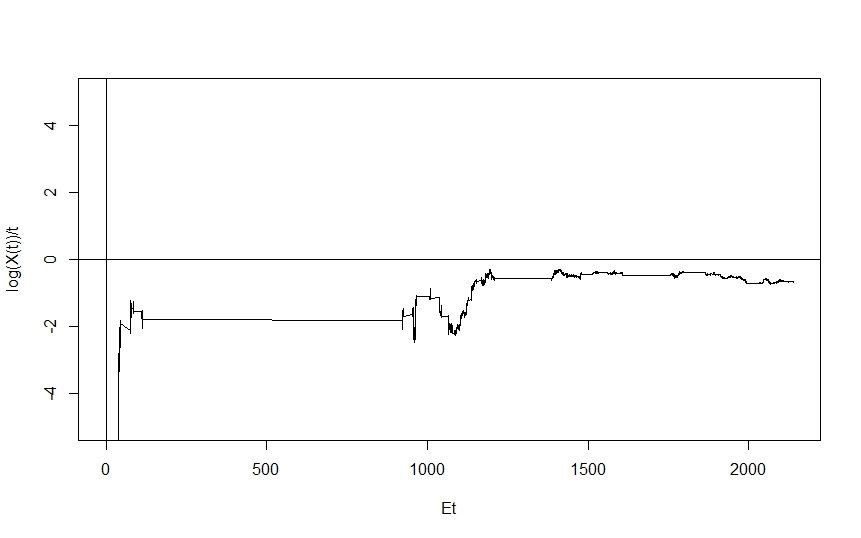
Figure 2. $\log(X(t))/E_{t}$ of SDE (3.20)

Remark 3.4.

Note that $f(x)=x^{\frac{3}{2}}$ fails to be a Lipschitz function and does not have linear growth condition. However, existence of unique solution to (3.20) is guaranteed by Theorem 3.5 on page 58 of Mao [9].

Remark 3.5.

In the figures of all examples, we assume that $E(t)$ is the inverse of stable subordinator with parameter $\alpha=.8$.

3.2. Stochastic Differential Equation (1.5) driven by Time-Changed Lévy Noise including Large Jumps

First, let us discuss exponential stability of the following time-changed SDE with noise that has only small linear jump

(3.24) $$dX(t) =f(t,E_{t},X(t-))dt+k(t,E_{t},X(t-))dE_{t}+g(t,E_{t},X(t-))dB_{E_{t}}$$

$$+\int_{|y|<c}h(y)X(t-)\tilde{N}(dE_{t},dy),$$

with $X(t_{0})=x_{0}$, which is a special case of (1.4) when $h(t_{1},t_{2},x,y)=h(x)y$. Then we extend (3.24) to (1.5) by adding large jumps $\int_{|y|\geq c}H(y)X(t-)N(dE_{t},dy)$ .

Assumption 3.6.

(3.25) $$Z_{c}=\int_{|y|<c}(|h(y)|\bigvee|h(y)|^{2})\nu(dy)<\infty,$$

for all $t_{1},t_{2}\in\mathbb{R^{+}}$.

Theorem 3.7.

Given Assumptions 2.7 and 3.6, suppose that there exist $\xi>0,\gamma\geq 0,\delta\geq 0,K_{1},K_{2}\in\mathbb{R}$ such that the following conditions

(3.26) $$(1)\gamma|x|^{2}\leq|g(t_{1},t_{2},x)|^{2}\leq\xi|x|^{2},\ (2)\int_{|y|<c}h(y)\nu(dy)\geq\delta$$

$$(3)f(t_{1},t_{2},x)x\leq K_{1}|x|^{2},\ (4)k(t_{1},t_{2},x)x\leq K_{2}|x|^{2}$$

are satisfied for all $x\in\mathbb{R}$ and $t_{1},t_{2}\in\mathbb{R^{+}}$. Then when $f\neq 0$ and $\lim_{t\to\infty}\frac{E_{t}}{t}=0$ a.s., we have

(3.27) $$\limsup_{t\rightarrow\infty}\frac{1}{t}\log|X(t)|\leq K_{1}\ a.s.$$

for any $x_{0}\neq 0$, the trivial solution of (3.24) is almost surely exponential path stable if $K_{1}<0$; when $f=0$, we have

(3.28) $$\limsup_{t\rightarrow\infty}\frac{1}{E_{t}}\log|X(t)|\leq-\Big{(}\gamma-K_{2}-\frac{\xi}{2}-\int_{|y|<c}\log(1+|h(y)|)\nu(dy)+\delta\Big{)}\ a.s.$$

for any $x_{0}\neq 0$, the trivial solution of (3.24) is almost surely path stable if $\gamma>K_{2}+\frac{\xi}{2}+\int_{|y|<c}\log(1+|h(y)|)\nu(dy)-\delta$.

Proof of Theorem 3.7.

Fix $x_{0}\neq 0$, then by Itô formula for time-changed SDE, see Lemma 3.1 in [12], we have

(3.29) $$\log(|X(t)|^{2})= \log(|x_{0}|^{2})+\int_{t_{0}}^{t}L_{1}\log(|X(s-)|^{2})ds+\int_{t_{0}}^{t}L_{2}\log(|X(s-)|^{2})dE_{s}$$

$$+\int_{t_{0}}^{t}\int_{|y|<c}\Big{[}\log(|X(s-)+X(s-)h(s,E_{s},y)|^{2})-\log(|X(s-)|^{2})\Big{]}\tilde{N}(dE_{s},dy)$$

$$+\int_{t_{0}}^{t}\int_{|y|<c}\frac{d}{dx}\log(|X(s-)|^{2})g(s,E_{s},X(s-))dB_{E_{s}},$$

where

(3.30) $$L_{1}\log(|X(s-)|^{2})=\frac{2X(s-)}{|X(s-)|^{2}}f(s,E_{s},X(s-))\leq 2K_{1},\\$$

(3.31) $$L_{2}\log(|X(s-)|^{2})dE_{s}= \frac{2X(s-)}{|X(s-)|^{2}}k(s,E_{s},X(s-))-\frac{|g(s,E_{s},X(s-))|^{2}}{|X(s-)|^{2}}$$

$$+\int_{|y|<c}\Big{[}\log(|X(s-)+h(y)X(s-)|^{2})-\log(|X(s-)|^{2})-2h(y)\Big{]}\nu(dy).$$

Applying condition (2) and Assumption 3.6 to (3.31),

(3.32) $$\int_{t_{0}}^{t}L_{2} \log(|X(s-)|^{2})dE_{s}=\int_{t_{0}}^{t}\Big{[}\frac{2X(s-)}{|X(s-)|^{2}}k(s,E_{s},X(s-))-\frac{|g(s,E_{s},X(s-))|^{2}}{|X(s-)|^{2}}\Big{]}dE_{s}$$

$$+ \int_{t_{0}}^{t}\Big{[}\int_{|y|<c}\big{[}\log(|X(s-)+h(y)X(s-)|^{2})-\log(|X(s-)|^{2})-2h(y)\big{]}\nu(dy)\Big{]}dE_{s}$$

$$\leq \int_{t_{0}}^{t}\Big{[}\frac{2K_{2}|X(s-)|^{2}}{|X(s-)|^{2}}+(\xi-2\gamma)\Big{]}dE_{s}+\int_{t_{0}}^{t}\Big{[}\int_{|y|<c}\big{[}\log((1+|h(y)|)^{2})\big{]}\nu(dy)-2\delta\Big{]}dE_{s}$$

$$\leq \int_{t_{0}}^{t}2K_{2}dE_{s}+2(E_{t}-E_{t_{0}})\int_{|y|<c}\Big{[}\log((1+|h(y)|))\Big{]}\nu(dy)$$

$$-(2\gamma+2\delta-\xi)(E_{t}-E_{t_{0}})$$

$$\leq (E_{t}-E_{t_{0}})\Big{[}2\int_{|y|<c}\log(1+|h(y)|)\nu(dy)+2K_{2}+\xi-2\gamma-2\delta\Big{]}$$

Note that both

(3.33) $$M_{1}(t)=\int_{t_{0}}^{t}\int_{|y|<c}\frac{d}{dx}\log(|X(s-)|^{2})g(s,E_{s},X(s-))dB_{E_{s}}$$

and

(3.34) $$M_{2}(t)=\int_{t_{0}}^{t}\int_{|y|<c}\Big{[}\log(|X(s-)+X(s-)h(y)|^{2})-\log(|X(s-)|^{2})\Big{]}\tilde{N}(dE_{s},dy)$$

are martingales.

Now,

(3.35) $$\log(|X(t)|^{2})\leq \log(|x_{0}|^{2})+2K_{1}(t-t_{0})+M_{1}(t)+M_{2}(t)$$

$$+(E_{t}-E_{t_{0}})\Big{(}2\int_{|y|<c}\log(1+|h(y)|)\nu(dy)+2K_{2}+\xi-2\gamma-2\delta\Big{)}.$$

Define corresponding non-time-changed stochastic process $\{z_{t}\}_{t\geq 0}$ by

(3.36) $$z(t)=z(t_{0})+\int_{t_{0}}^{t}f(s,z(s-))dt+\int_{t_{0}}^{t}g(s,z(s-))dB(t)+\int_{t_{0}}^{t}\int_{|y|<c}h(y)z(s-)\tilde{N}(ds,dy),$$

with $z(t_{0})=x_{0}$. By the duality theorem 4.2 in [6], $X(t)=z(E_{t})$ for $t\geq t_{0}$.

By the result on page 282 in Mao [9],

(3.37) $$\langle M_{1}\rangle(t)= \langle 2\int_{E_{t_{0}}}^{E_{t}}\frac{z(s-)g(s,z(s-))}{|z(s-)|^{2}}dB_{k}(s)\rangle$$

$$= 4\int_{E_{t_{0}}}^{E_{t}}\frac{|z(s-)g(s,z(s-))|^{2}}{|z(s-)|^{4}}ds$$

$$\leq 4\xi(E_{t}-E_{t_{0}}).$$

Define $\rho_{M_{1}}(t)=\int_{t_{0}}^{t}\frac{d\langle M_{1}\rangle(s)}{(1+E_{s})^{2}}$, then

(3.38) $$\rho_{M_{1}}(t)\leq 4\xi\int_{t_{0}}^{t}\frac{dE_{s}}{(1+E_{s})^{2}}=4\xi\int_{E_{t_{0}}}^{E_{t}}\frac{ds}{(1+s)^{2}}=\frac{-4\xi}{1+s}\Big{|}_{E_{t_{0}}}^{E_{t}}=4\xi\big{[}\frac{1}{1+{E_{t_{0}}}}-\frac{1}{1+E_{t}}\big{]},$$

then

(3.39) $$\lim_{t\rightarrow\infty}\rho_{M_{1}}(t)\leq\lim_{t\rightarrow\infty}4\xi\big{[}\frac{1}{1+{E_{t_{0}}}}-\frac{1}{1+E_{t}}\big{]})\leq 4\xi<\infty.$$

By Theorem 10 of Chapter 2 in [7],

(3.40) $$\lim_{t\rightarrow\infty}\frac{M_{1}(t)}{E_{t}}=0,\ a.s..$$

Similarly,

(3.41) $$\langle M_{2}\rangle(t)= \int_{E_{t_{0}}}^{E_{t}}\int_{|y|<c}[\log(\frac{z(s-)+z(s-)h(y)}{|z(s-)|^{2}})]^{2}\nu(dy)ds$$

$$\leq \int_{E_{t_{0}}}^{E_{t}}\int_{|y|<c}[\log((1+|h(y)|)^{2})]^{2}\nu(dy)ds$$

$$\leq 4\int_{E_{t_{0}}}^{E_{t}}\int_{|y|<c}|h(y)|^{2}\nu(dy)ds$$

$$\leq 4Z_{c}(E_{t}-E_{t_{0}}),$$

so

(3.42) $$\lim_{t\rightarrow\infty}\rho_{M_{2}}(t)\leq\lim_{t\rightarrow\infty}4Z_{c}\int_{t_{0}}^{t}\frac{dE_{s}}{(1+E_{s})^{2}}<\infty\ a.s..$$

As a result,

(3.43) $$\lim_{t\rightarrow\infty}\frac{M_{2}(t)}{E_{t}}=0,\ a.s..$$

In the end, since

(3.44) $$\lim_{t\rightarrow\infty}\frac{E_{t}}{t}=0,\ a.s.,$$

and

(3.45) $$\frac{\log|X(t)|}{t}\leq \frac{\log|x_{0}|}{t}+\frac{2K_{1}(t-t_{0})}{t}+\frac{(E_{t}-E_{t_{0}})(\int_{|y|<c}\log(1+|h(y)|)\nu(dy)+K_{2}+\frac{\xi}{2}-\gamma-\delta)}{t}$$

$$+ \frac{M_{1}(t)}{2E_{t}}\frac{E_{t}}{t}+\frac{M_{2}(t)}{2E_{t}}\frac{E_{t}}{t}$$

thus,

(3.46) $$\limsup_{t\rightarrow\infty}\frac{\log|X(t)|}{t}\leq K_{1}\ a.s..$$

When $f=0$,

(3.47) $$\frac{\log|X(t)|}{E_{t}}\leq\frac{\log|x_{0}|}{E_{t}}+\frac{(E_{t}-E_{t_{0}})(\int_{|y|<c}\log(1+|h(y)|)\nu(dy)+K_{2}+\frac{\xi}{2}-\gamma-\delta)}{E_{t}}+\frac{M_{1}(t)}{2E_{t}}+\frac{M_{2}(t)}{2E_{t}}$$

thus,

(3.48) $$\limsup_{t\rightarrow\infty}\frac{\log|X(t)|}{E_{t}}\leq\int_{|y|<c}\log(1+|h(y)|)\nu(dy)+K_{2}+\frac{\xi}{2}-\gamma-\delta\ a.s..$$

∎

Other than the direct proof above, the following is an alternative proof utilizing Theorem 3.1.

Alternate Proof of Theorem 3.7.

Let $V(x)=|x|^{2}$, then $V\in C^{2}(\mathbb{R},\mathbb{R}^{+})$ and condition (i) in Theorem 3.1 is satisfied.

Next, by applying the time-changed Itô formula to $V(X(t))$, $L_{1}V(x)=f(t_{1},t_{2},x)2x\leq 2K_{1}V(x)$, thus condition (ii) in Theorem 3.1 is satisfied;

(3.49) $$L_{2}V(x) =k(t_{1},t_{2},x)2x+|g(t_{1},t_{2},x)|^{2}+\int_{|y|<c}\Big{[}|x+h(y)x|^{2}-|x|^{2}-h(y)x2x\Big{]}\nu(dy)$$

$$\leq 2K_{2}|x|^{2}+|g(t_{1},t_{2},x)|^{2}+\int_{|y|<c}|x|^{2}\Big{[}(1+h(y))^{2}-1-2h(y)\Big{]}\nu(dy)$$

$$\leq\Big{[}2K_{2}+\xi+\int_{|y|<c}|h(y)|^{2}\nu(dy)\Big{]}|x|^{2}<\infty,$$

thus, condition (iii) in Theorem 3.1 is satisfied by Assumption 3.6 and setting $c_{3}=2K_{2}+\xi+\int_{|y|<c}|h(y)|^{2}\nu(dy)$.

Condition (iv) is satisfied since

(3.50) $$|(\partial_{x}V(x))g(t_{1},t_{2},x)|^{2}=|2xg(t_{1},t_{2},x)|^{2}\geq 4\gamma|x|^{4}.$$

For the last condition (v), by denoting $c_{5}=-\int_{|y|<c}\Big{[}\log(1+|h(y)|)-|h(y)|^{2}\Big{]}\nu(dy)-2\delta$ we have

(3.51) $$\int_{|y|<c}\Big{[}\log\Big{(}\frac{V(x+h(y)x)}{V(x)}\Big{)}-\frac{V(x+h(y)x)-V(x)}{V(x)}\Big{]}\nu(dy)$$

$$= \int_{|y|<c}\Big{[}\log\Big{(}\frac{|x+h(y)x|^{2}}{|x|^{2}}\Big{)}-\frac{|x+h(y)x|^{2}-|x|^{2}}{|x|^{2}}\Big{]}\nu(dy)$$

$$\leq \int_{|y|<c}\Big{[}\log(1+|h(y)|)-\frac{2xh(y)x+|h(y)x|^{2}}{|x|^{2}}\Big{]}\nu(dy)$$

$$\leq \int_{|y|<c}\Big{[}\log(1+|h(y)|)-|h(y)|^{2}\Big{]}\nu(dy)-2\delta<0.$$

Since all five conditions in Theorem 3.1 are satisfied, we have that when $f\neq 0$,

(3.52) $$\limsup_{t\rightarrow\infty}\frac{1}{t}\log|X(t)|\leq K_{1}\ \ a.s.;$$

and that when $f=0$,

(3.53) $$\limsup_{t\rightarrow\infty} \frac{1}{E_{t}}\log|X(t)|$$

$$\leq\frac{1}{2}\Big{(}2K_{2}+\xi-\int_{|y|<c}|h(y)|^{2}\nu(dy)-\frac{4\gamma}{2}-\int_{|y|<c}\Big{[}\log(1+|h(y)|)-|h(y)|^{2}\Big{]}\nu(dy)-2\delta\Big{)}$$

$$=-\Big{(}-K_{2}-\frac{\xi}{2}+\gamma-\int_{|y|<c}\Big{[}\log(1+|h(y)|_{1})\Big{]}\nu(dy))+\delta\Big{)}\ \ a.s.$$

as desired.

∎

Example 3.8.

Consider the following stochastic differential equation

(3.54) $$dX(t)=-sin(X(t-))X(t-)dE_{t}+\frac{X(t-)}{E_{t}+1}dB_{E_{t}}+\int_{|y|\leq 1}16X(t-)y^{2}\tilde{N}(dE_{t},dy),$$

with $X(0)=1$, $\nu$ is uniform distribution $[0,1]$.

Applying Theorem 3.7, $0\leq|g(x,t_{1},t_{2})^{2}|\leq|x|^{2}$, $\int_{|y|\leq 1}h(y)\nu(dy)\geq\frac{16}{3}$ and $k(t_{1},t_{2},x)x\leq|x|^{2}$, thus $\gamma=0,\ \xi=1,\ \delta=\frac{16}{3},\ K_{2}=1$.

(3.55) $$\limsup_{t\rightarrow\infty}\frac{1}{E_{t}}\log|X(t)| \leq-\Big{(}\gamma-K_{2}-\frac{\xi}{2}-\int_{|y|<c}\log(1+|h(y)|)\nu(dy)+\delta\Big{)}$$

$$=-(0-1-\frac{1}{2}-\log(17)+\frac{16}{3})<0\ a.s..$$

Hence, stochastic differential equation (3.54) is almost surely path stable. The simulated path of SDE (3.54) is given in Figure 3. The ratio of $\frac{\log|X(t)|}{E_{t}}$ is strictly below $0$ for large time t, this is consistent with above analysis.

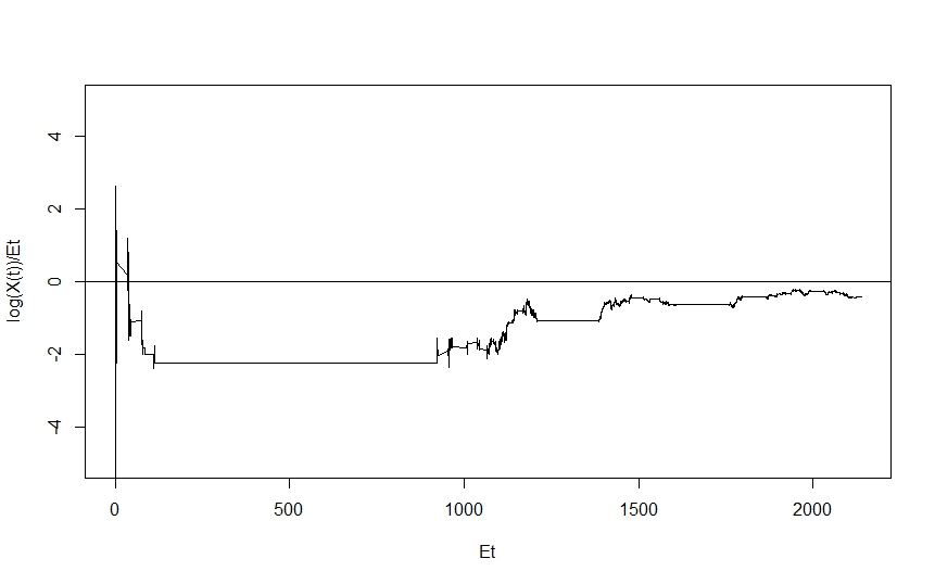
Figure 3. $\log(X(t))/E_{t}$ of SDE (3.54)

Next, we analyze the following time-changed stochastic differential equation involving large jumps,

(3.56) $$dX(t)=\int_{|y|\geq c}H(y)X(t-)N(dE_{t},dy),$$

with $X(t_{0})=x_{0}\in\mathbb{R}$ and $H:\mathbb{R}\rightarrow\mathbb{R}$ is a measurable function.

Before stating the next theorem, we need another assumption, see [14].

Assumption 3.9.

Assume that

(3.57) $$\int_{|y|\geq c}||H(y)||_{1}^{2}\nu(dy)<\infty$$

and that $H(y)\neq-1$ for $|y|\geq c$.

By above assumption, the function $H(y)x$ satisfies Lipschitz and growth conditions, assuring the existence and uniqueness of solution to equation (3.56). In addition, $H(y)\neq-1$ implies that $P(X(t)\neq 0\ for\ all\ t\geq t_{0})=1$, this is an application of interlacing technique in [1], details can be found in Lemma 4.3.2 in [14] with simple modification.

Theorem 3.10.

If

(3.58) $$\sup_{x\in\mathbb{R}-0}\int_{|y|\geq c}\Big{[}\log(|x+H(y)x|)-\log(|x|)\Big{]}\nu(dy)<-K,$$

for some $K>0$, then the sample Lyapunov exponent of solution of (3.56) exists and satisfies

(3.59) $$\limsup_{t\rightarrow\infty}\frac{1}{E_{t}}\log|X(t)|\leq-2K\ \ a.s.,$$

for any $x_{0}\neq 0$, that is, the trivial solution of (3.56) is almost surely path stable.

Proof.

Fix $x_{0}\neq 0$, apply Itô formula (2.12) to $\log(|X(t)|^{2})$, then for any $t\geq 0$,

(3.60) $$\log(|X(t)|^{2})= \log(x_{0}^{2})+\int_{t_{0}}^{t}\int_{|y|\geq c}\Big{[}\log(|X(s)+H(y)X(s)|^{2})-\log(|X(s)|^{2})\Big{]}N(dE_{s},dy)$$

$$= \log(x_{0}^{2})+\int_{t_{0}}^{t}\int_{|y|\geq c}\Big{[}\log(|X(s)+H(y)X(s)|^{2})-\log(|X(s)|^{2})\Big{]}\tilde{N}(dE_{s},dy)$$

$$+\int_{t_{0}}^{t}\int_{|y|\geq c}\Big{[}\log(|X(s)+H(y)X(s)|^{2})-\log(|X(s)|^{2})\Big{]}\nu(dy)dE_{s}.$$

Let $M_{3}(t)=\int_{t_{0}}^{t}\int_{|y|\geq c}\Big{[}\log(|X(s)+H(y)X(s)|^{2})-\log(|X(s)|^{2})\Big{]}\tilde{N}(dE_{s},dy)$, similar ideas as in the proof of the corresponding inequality for $M_{2}(t)$ in the proof of Theorem (3.7), we have

(3.61) $$\lim_{t\rightarrow\infty}\frac{M_{3}(t)}{E_{t}}=0,\ \ a.s.,$$

thus

(3.62) $$\frac{\log(|X(t)|^{2})}{E_{t}}\leq \frac{\log(x_{0}^{2})}{E_{t}}+\frac{(E_{t}-E_{t_{0}})\sup_{0\leq s\leq t}\int_{|y|\geq c}\Big{[}\log(|X(s)+H(y)X(s)|^{2})-\log(|X(s)|^{2})\Big{]}\nu(dy)}{E_{t}}$$

$$\rightarrow \sup_{0\leq s\leq t}\int_{|y|\geq c}\Big{[}\log(|X(s)+H(y)X(s)|^{2})-\log(|X(s)|^{2})\Big{]}\nu(dy)\leq-2K,\ as\ t\rightarrow\infty.$$

∎

Next, by similar ideas as the proof of Theorem 4.6.1 in [14], it is not difficult to derive the following theorem for the following time-changed SDE

(3.63) $$dX(t) =f(t,E_{t},X(t-))dt+k(t,E_{t},X(t-))dE_{t}+g(t,E_{t},X(t-))dB_{E_{t}}$$

$$+\int_{|y|<c}h(y)X(t-)\tilde{N}(dE_{t},dy)+\int_{|y|\geq c}H(y)X(t-)N(dE_{t},dy).$$

with $X(t_{0})=x_{0}$.

Theorem 3.11.

Given assumptions 2.7, 3.6 and 3.9, suppose that there exist $\xi>0,\gamma\geq 0,\delta\geq 0,K_{1},K_{2}\in\mathbb{R}$ such that the following conditions

(3.64) $$(1)\gamma|x|^{2}\leq|g(t_{1},t_{2},x)|^{2}\leq\xi|x|^{2},\ (2)\int_{|y|<c}h(y)\nu(dy)\geq\delta$$

$$(3)f(t_{1},t_{2},x)x\leq K_{1}|x|^{2},\ (4)k(t_{1},t_{2},x)x\leq K_{2}|x|^{2}$$

are satisfied for all $x\in\mathbb{R}$ and $t_{1},t_{2}\in\mathbb{R^{+}}$. Then when $f\neq 0$and $\lim_{t\to\infty}\frac{E_{t}}{t}=0$ a.s., we have

(3.65) $$\limsup_{t\rightarrow\infty}\frac{1}{t}\log|X(t)|\leq K_{1}\ a.s.,$$

for any $x_{0}\neq 0$, the trivial solution of (1.5) is almost surely exponentially path stable if $K_{1}<0$; when $f=0$, we have

(3.66) $$\limsup_{t\rightarrow\infty}\frac{1}{E_{t}}\log|x(t)|\leq-\Big{(}\gamma-K_{2}-\frac{\xi}{2}-\int_{|y|<c}\log(1+|h(y)|)\nu(dy)+\delta-M(c)\Big{)}\ a.s.,$$

where $M(c)=\sup_{x\in\mathbb{R}-\{0\}}\int_{|y|\geq c}\Big{[}\log(|x+H(y)x|)-\log(|x|)\Big{]}\nu(dy)<\infty$, for any $x_{0}\neq 0$, and the trivial solution of (1.5) is almost surely path stable if $\gamma>K_{2}+\frac{\xi}{2}+\int_{|y|<c}\log(1+|h(y)|)\nu(dy)-\delta+M(c)$.

Proof.

Application of Theorem 3.1 and Theorem 3.10. ∎

Remark 3.12.

The Theorems 3.1 and 3.11 show that the coefficient of $"dt"$ (i.e. the drift term) plays the dominating role in determining the almost sure exponential path stabilities. In absence the of $"dt"$ part, almost sure path stability is the result of the coefficients of the other components.

Next, we list some examples to illustrate the results of above theorems.

Example 3.13.

Consider the following two stochastic differential equations

(3.67) $$dX(t)=X(t-)dt+X(t-)dB_{E_{t}}+\int_{0}^{t}\int_{|y|\leq 1}X(t-)y^{2}\tilde{N}(dE_{t},dy)+\int_{0}^{t}\int_{|y|>1}X(t-)y^{2}N(dE_{t},dy)$$

with $X(0)=.1$ and $\nu$ is standard normal distribution,

and

(3.68) $$dX(t)=-X(t-)dt+ X(t-)dB_{E_{t}}$$

$$+2\int_{0}^{t}\int_{|y|\leq 1}X(t-)y^{2}\tilde{N}(dE_{t},dy)+2\int_{0}^{t}\int_{|y|>1}X(t-)y^{2}N(dE_{t},dy)$$

with $X(0)=.1$ and $\nu$ is standard normal distribution.

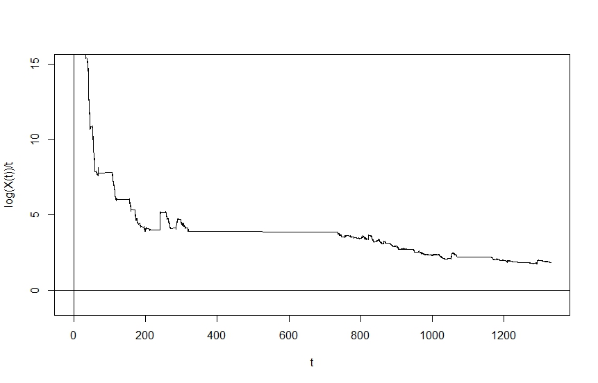
Figure 4. $\log(X(t))/t$ of SDE (3.67)

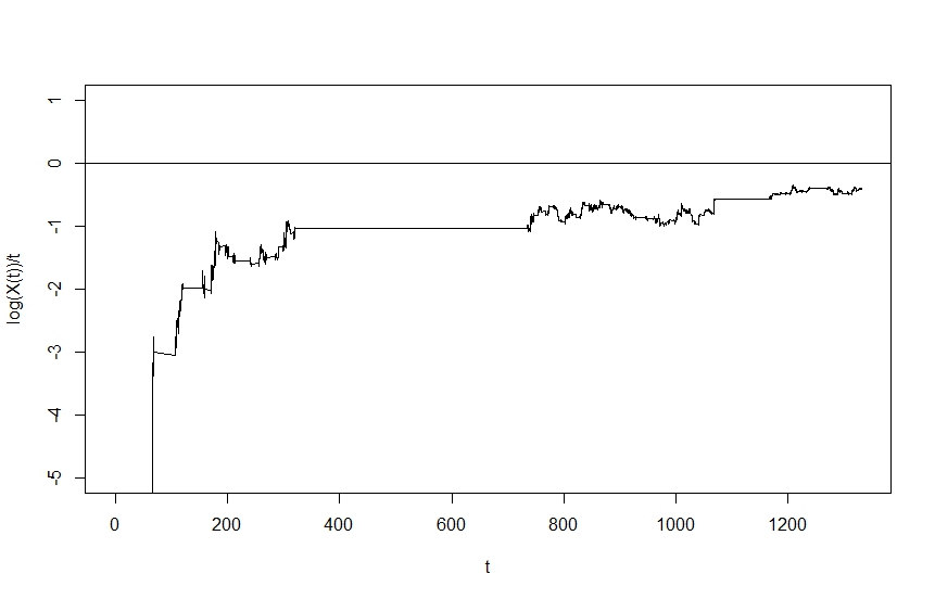
Figure 5. $\log(X(t))/t$ of SDE (3.68)

Figure 4 illustrates that stochastic differential equation (3.67) is not almost surely exponentially path stable, this is because ”dt” component exists in the linear stochastic system, such component plays dominant role in determining almost sure exponential path stability and has positive scalar 1, thus $\limsup_{t\rightarrow\infty}\frac{1}{t}\log|x(t)|\leq 1$, this is not enough for almost sure exponential path stability.

In contrast, as illustrated in the Figure 5, (also verified by Theorem 3.11) stochastic differential equation (3.68) is almost surely exponentially stable. This is because that coefficient for $dt$ in (3.68) is -1, thus $\limsup_{t\rightarrow\infty}\frac{1}{t}\log|x(t)|\leq-1$, this implies almost sure exponential path stability.

Example 3.14.

Consider following two stochastic differential equations

(3.69) $$dX(t)=-X(t-)dE_{t}+ X(t-)dB_{E_{t}}$$

$$+\int_{0}^{t}\int_{|y|\leq 1}X(t-)y^{2}\tilde{N}(dE_{t},dy)+\int_{0}^{t}\int_{|y|>1}X(t-)y^{2}N(dE_{t},dy)$$

with $X(0)=-3$, and

(3.70) $$dX(t)=-X(t-)dE_{t}+ 2X(t-)dB_{E_{t}}$$

$$+\int_{0}^{t}\int_{|y|\leq 1}X(t-)y^{2}\tilde{N}(dE_{t},dy)+\int_{0}^{t}\int_{|y|>1}X(t-)y^{2}N(dE_{t},dy)$$

with $X(0)=-3$.

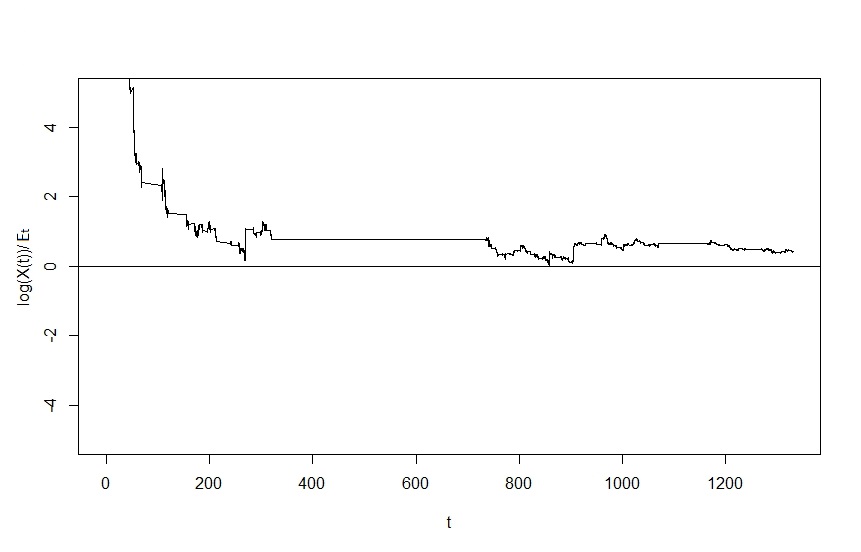
Figure 6. $\log(X(t))/E_{t}$ of SDE (3.69)

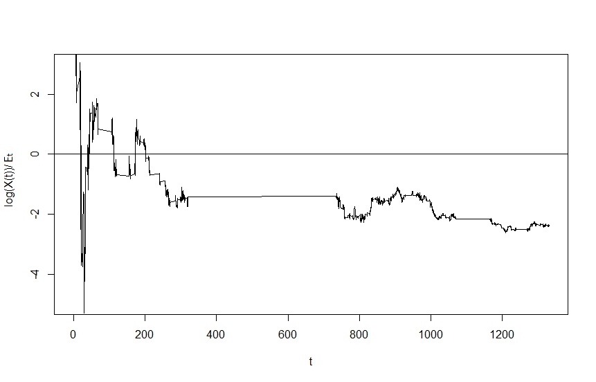
Figure 7. $\log(X(t))/E_{t}$ of SDE (3.70)

In both of the equations (3.69) and (3.70), $"dt"$ component is missing, thus almost sure exponential path stability is no longer possible. However, almost sure path stability is possible, depending on the scalars of time-changed drift, Brownian motion, and Possion jump.

In stochastic differential equations (3.69), the corresponding parameters are $K_{2}=\xi=\gamma=1$, $\delta=.2$, $h(y)=H(y)=y^{2}$ and $0\leq\delta\leq\int_{|y|<1}y^{2}\nu(dy)<1$, by Theorem 3.11

(3.71) $$\limsup_{t\rightarrow\infty} \frac{1}{E_{t}}\log|X(t)|$$

$$<-\Big{(}1-1-\frac{1}{2}-\int_{|y|<1}\log(1+y^{2})\nu(dy)+.2-\sup_{x\in\mathbb{R}^{d}-0}\int_{|y|<1}\log(1+y^{2})\nu(dy)\Big{)}$$

$$\leq\int_{|y|<1}\log(1+y^{2})\nu(dy)+.3\ \ \ a.s.,$$

which is not enough to conclude the almost sure path stability of stochastic differential equations (3.69).

However, in stochastic differential equations (3.70) corresponding parameters are $K_{2}=1,\ \delta=.2,\ \gamma=\xi=4$, $h(y)=H(y)=y^{2}$ and $0\leq\delta\leq\int_{|y|<1}y^{2}\nu(dy)<1$, by Theorem 3.11

(3.72) $$\limsup_{t\rightarrow\infty} \frac{1}{E_{t}}\log|X(t)|$$

$$<-\Big{(}4-1-2-\int_{|y|<1}\log(1+y^{2})\nu(dy)+.2-\sup_{x\in\mathbb{R}^{d}-0}\int_{|y|<1}\log(1+y^{2})\nu(dy)\Big{)}$$

$$\leq-.8+2\int_{|y|<1}\log(1+y^{2})\nu(dy)\leq-.8+2\int_{|y|<1}y^{2}\nu(dy)\leq 0\ \ \ a.s.,$$

thus the solution of stochastic differential equation (3.70) is almost surely path stable.

References

- [1] D. Applebaum. Lévy processes and stochastic calculus, Cambridge University Press, 2009.
- [2] W. Feller. An Introduction to Probability Theory and Its Applications, 2nd ed., vol. II, Wiley, New York, 1971.
- [3] J. Janczura and A. Wyloma nska. Subdynamics of financial data from fractional Fokker-Planck equation, Acta Physica Polonica B 40 (2009) 1341 -1351.
- [4] S.K. Jha, C.J. Langmead. Exploring behaviors of stochastic differential equation models of biological systems using change of measures, BMC bioinformatics Vol 13 (2012): 1.
- [5] E. Jum, and K. Kobayashi. A strong and weak approximation scheme for stochastic differential equations driven by a time-changed Brownian motion, arXiv preprint arXiv:1408.4377, (2014).
- [6] K. Kobayashi. Stochastic calculus for a time-changed semimartingale and the associated stochastic differential equations, Journal of Theoretical Probability 24.3 (2011): 789–820.
- [7] R.Sh. Liptser and A.N. Shiryayev. Theory of martingales, Kluwer Academic Publishers Group, Dordrecht, 1989.
- [8] A. M. Lyapunov. The general problem of the stability of motion, International Journal of Control 55.3 (1992): 531–534.
- [9] X. Mao. Stochastic differential equations and applications, Horwood Publishing Limited, Chichester, 2008.
- [10] M. M. Meerschaert and H. P. Scheffler. Stochastic model for ultraslow diffusion, Stochastic processes and their applications 116.9 (2006): 1215–1235.
- [11] R.C. Merton. Option pricing when underlying stock returns are discontinuous, Journal of financial economics 3.1-2 (1976): 125–144.
- [12] E. Nane and Y. Ni. Stability of stochastic differential equation driven by time-changed Lévy noise, Proceedings of the American Mathematical Society (to appear), 2016.
- [13] F. Shokrollahi, A. Kilicman and M. Magdziarz. Pricing European options and currency options by time changed mixed fractional Brownian motion with transaction costs, International Journal of Financial Engineering, Vol 3 (2016), no.1, 1650003 (20 pages).
- [14] M. Siakalli. Stability properties of stochastic differential equations driven by L vy noise, Diss. University of Sheffield, 2009.
- [15] Q. Wu. Stability of stochastic differential equations with respect to time-changed Brownian motions, arXiv preprint arXiv:1602.08160 (2016).