Geometric Descent Method for Convex Composite Minimization

Abstract

In this paper, we extend the geometric descent method recently proposed by Bubeck, Lee and Singh [1] to tackle nonsmooth and strongly convex composite problems. We prove that our proposed algorithm, dubbed geometric proximal gradient method (GeoPG), converges with a linear rate $(1-1/\sqrt{\kappa})$ and thus achieves the optimal rate among first-order methods, where $\kappa$ is the condition number of the problem. Numerical results on linear regression and logistic regression with elastic net regularization show that GeoPG compares favorably with Nesterov’s accelerated proximal gradient method, especially when the problem is ill-conditioned.

1 Introduction

Recently, Bubeck, Lee and Singh proposed a geometric descent method (GeoD) for minimizing a smooth and strongly convex function [1]. They showed that GeoD achieves the same optimal rate as Nesterov’s accelerated gradient method (AGM) [2, 3]. In this paper, we provide an extension of GeoD that minimizes a nonsmooth function in the composite form:

$$\min_{x\in\mathbb{R}^{n}}\ F(x):=f(x)+h(x),$$ (1.1)

where $f$ is $\alpha$-strongly convex and $\beta$-smooth (i.e., $\nabla f$ is Lipschitz continuous with Lipschitz constant $\beta$), and $h$ is a closed nonsmooth convex function with simple proximal mapping. Commonly seen examples of $h$ include $\ell_{1}$ norm, $\ell_{2}$ norm, nuclear norm, and so on.

If $h$ vanishes, then the objective function of (1.1) becomes smooth and strongly convex. In this case, it is known that AGM converges with a linear rate $(1-1/\sqrt{\kappa})$, which is optimal among all first-order methods, where $\kappa=\beta/\alpha$ is the condition number of the problem. However, AGM lacks a clear geometric intuition, making it difficult to interpret. Recently, there has been much work on attempting to explain AGM or designing new algorithms with the same optimal rate (see, [4, 5, 1, 6, 7]). In particular, the GeoD method proposed in [1] has a clear geometric intuition that is in the flavor of the ellipsoid method [8]. The follow-up work [9, 10] attempted to improve the performance of GeoD by exploiting the gradient information from the past with a “limited-memory” idea. Moreover, Drusvyatskiy, Fazel and Roy [10] showed how to extend the suboptimal version of GeoD (with the convergence rate $(1-1/\kappa)$) to solve the composite problem (1.1). However, it was not clear how to extend the optimal version of GeoD to address (1.1), and the authors posed this as an open question. In this paper, we settle this question by proposing a geometric proximal gradient (GeoPG) algorithm which can solve the composite problem (1.1). We further show how to incorporate various techniques to improve the performance of the proposed algorithm.

Notation. We use $B(c,r^{2})=\left\{x|\|x-c\|^{2}\leq r^{2}\right\}$ to denote the ball with center $c$ and radius $r$. We use $\mathop{\rm Line}(x,y)$ to denote the line that connects $x$ and $y$, i.e., $\{x+s(y-x),s\in\mathbb{R}\}$. For fixed $t\in(0,1/\beta]$, we denote $x^{+}:={\rm Prox}_{th}(x-t\nabla f(x))$, where the proximal mapping ${\rm Prox}_{h}(\cdot)$ is defined as ${\rm Prox}_{h}(x):=\mathop{\rm argmin}_{z}\ h(z)+\frac{1}{2}\|z-x\|^{2}$. The proximal gradient of $F$ is defined as $G_{t}(x):=(x-x^{+})/t$. It should be noted that $x^{+}=x-tG_{t}(x)$. We also denote $x^{++}:=x-G_{t}(x)/\alpha$. Note that both $x^{+}$ and $x^{++}$ are related to $t$, and we omit $t$ whenever there is no ambiguity.

The rest of this paper is organized as follows. In Section 2, we briefly review the GeoD method for solving smooth and strongly convex problems. In Section 3, we provide our GeoPG algorithm for solving nonsmooth problem (1.1) and analyze its convergence rate. We address two practical issues of the proposed method in Section 4, and incorporate two techniques: backtracking and limited memory, to cope with these issues. In Section C, we report some numerical results of comparing GeoPG with Nesterov’s accelerated proximal gradient method in solving linear regression and logistic regression problems with elastic net regularization. Finally, we conclude the paper in Section 6.

2 Geometric Descent Method for Smooth Problems

The GeoD method [1] solves (1.1) when $h\equiv 0$, in which the problem reduces to a smooth and strongly convex problem $\min\ f(x)$. We denote its optimal solution and optimal value as $x^{*}$ and $f^{*}$, respectively. Throughout this section, we fix $t=1/\beta$, which together with $h\equiv 0$ implies that $x^{+}=x-\nabla f(x)/\beta$ and $x^{++}=x-\nabla f(x)/\alpha$. We first briefly describe the basic idea of the suboptimal GeoD. Since $f$ is $\alpha$-strongly convex, the following inequality holds

$$f(x)+\langle\nabla f(x),y-x\rangle+\frac{\alpha}{2}\|y-x\|^{2}\leq f(y),\ \forall x,y\in\mathbb{R}^{n}.$$ (2.1)

By letting $y=x^{*}$ in (B.2), one obtains that

$$x^{*}\in B\big{(}x^{++},\|\nabla f(x)\|^{2}/\alpha^{2}-2(f(x)-f^{*})/\alpha\big{)},\forall x\in\mathbb{R}^{n}.$$ (2.2)

Note that the $\beta$-smoothness of $f$ implies

$$f(x^{+})\leq f(x)-\|\nabla f(x)\|^{2}/(2\beta),\forall x\in\mathbb{R}^{n}.$$ (2.3)

Combining (2.2) and (2.3) yields $x^{*}\in B\big{(}x^{++},(1-1/\kappa)\|\nabla f(x)\|^{2}/\alpha^{2}-2(f(x^{+})-f^{*})/\alpha\big{)}.$ As a result, suppose that initially we have a ball $B(x_{0},R_{0}^{2})$ that contains $x^{*}$, then it follows that

$$x^{*}\in B\big{(}x_{0},R_{0}^{2}\big{)}\cap B\big{(}x_{0}^{++},(1-1/\kappa)\|\nabla f(x_{0})\|^{2}/\alpha^{2}-2(f(x_{0}^{+})-f^{*})/\alpha\big{)}.$$ (2.4)

Some simple algebraic calculations show that the squared radius of the minimum enclosing ball of the right hand side of (2.4) is no larger than $R_{0}^{2}(1-1/\kappa)$, i.e., there exists some $x_{1}\in\mathbb{R}^{n}$ such that $x^{*}\in B\big{(}x_{1},R_{0}^{2}(1-1/\kappa)\big{)}$. Therefore, the squared radius of the initial ball shrinks by a factor $(1-1/\kappa)$. Repeating this process yields a linear convergent sequence $\{x_{k}\}$ with the convergence rate $(1-1/\kappa)$: $\|x_{k}-x^{*}\|^{2}\leq(1-1/\kappa)^{k}R_{0}^{2}.$

The optimal GeoD (with the linear convergence rate $(1-1/\sqrt{\kappa})$) maintains two balls containing $x^{*}$ in each iteration, whose centers are $c_{k}$ and $x_{k+1}^{++}$, respectively. More specifically, suppose that in the $k$-th iteration we have $c_{k}$ and $x_{k}$, then $c_{k+1}$ and $x_{k+1}$ are obtained as follows. First, $x_{k+1}$ is the minimizer of $f$ on $\mathop{\rm Line}(c_{k},x_{k}^{+})$. Second, $c_{k+1}$ (resp. $R_{k+1}^{2}$) is the center (resp. squared radius) of the ball (given by Lemma 2.1) that contains

$$B(c_{k},R_{k}^{2}-\|\nabla f(x_{k+1})\|^{2}/(\alpha^{2}\kappa))\cap B(x_{k+1}^{++},(1-1/\kappa)\|\nabla f(x_{k+1})\|^{2}/\alpha^{2}).$$

Calculating $c_{k+1}$ and $R_{k+1}$ is easy and we refer to Algorithm 1 of [1] for details. By applying Lemma 2.1 with $x_{A}=c_{k}$, $r_{A}=R_{k}$, $r_{B}=\|\nabla f(x_{k+1})\|/\alpha$, $\epsilon=1/\kappa$ and $\delta=\frac{2}{\alpha}(f(x_{k}^{+})-f(x^{*}))$, we obtain $R_{k+1}^{2}=(1-1/\sqrt{\kappa})R_{k}^{2}$, which further implies $\|x^{*}-c_{k}\|^{2}\leq(1-1/\sqrt{\kappa})^{k}R_{0}^{2},$ i.e., the optimal GeoD converges with the linear rate $(1-1/\sqrt{\kappa})$.

Lemma 2.1 (see [1, 10]).

Fix centers $x_{A}$, $x_{B}\in\mathbb{R}^{n}$ and squared radii $r_{A}^{2},r_{B}^{2}>0$. Also fix $\epsilon\in(0,1)$ and suppose $\|x_{A}-x_{B}\|^{2}\geq r_{B}^{2}$. There exists a new center $c\in\mathbb{R}^{n}$ such that for any $\delta>0$, we have

$$B(x_{A},r_{A}^{2}-\epsilon r_{B}^{2}-\delta)\cap B\big{(}x_{B},r_{B}^{2}(1-\epsilon)-\delta\big{)}\subset B\big{(}c,(1-\sqrt{\epsilon})r_{A}^{2}-\delta\big{)}.$$

3 Geometric Descent Method for Convex Nonsmooth Composite Problems

Drusvyatskiy, Fazel and Roy [10] extended the suboptimal GeoD to solve the composite problem (1.1). However, it was not clear how to extend the optimal GeoD to solve problem (1.1). We resolve this problem in this section.

The following lemma is useful to our analysis. Its proof is in the appendix.

Lemma 3.1.

Given point $x\in\mathbb{R}^{n}$ and step size $t\in(0,1/\beta]$, denote $x^{+}=x-tG_{t}(x)$. The following inequality holds for any $y\in\mathbb{R}^{n}$:

$$F(y)\geq F(x^{+})+\langle G_{t}(x),y-x\rangle+\frac{t}{2}\|G_{t}(x)\|^{2}+\frac{\alpha}{2}\|y-x\|^{2}.$$ (3.1)

3.1 GeoPG Algorithm

In this subsection, we describe our proposed geometric proximal gradient method (GeoPG) for solving (1.1). Throughout Sections 3.1 and 3.2, $t\in(0,1/\beta]$ is a fixed scalar. The key observation for designing GeoPG is that in the $k$-th iteration one has to find $x_{k}$ that lies on $\mathop{\rm Line}(x_{k-1}^{+},c_{k-1})$ such that the following two inequalities hold:

$$F(x_{k}^{+})\leq F(x_{k-1}^{+})-\frac{t}{2}\|G_{t}(x_{k})\|^{2},\mbox{ and }\|x_{k}^{++}-c_{k-1}\|^{2}\geq\frac{1}{\alpha^{2}}\|G_{t}(x_{k})\|^{2}.$$ (3.2)

Intuitively, the first inequality in (3.2) requires that there is a function value reduction on $x_{k}^{+}$ from $x_{k-1}^{+}$, and the second inequality requires that the centers of the two balls are far away from each other so that Lemma 2.1 can be applied.

The following lemma gives a sufficient condition for (3.2). Its proof is in the appendix.

Lemma 3.2.

(3.2) holds if $x_{k}$ satisfies

$$\langle x_{k}^{+}-x_{k},x_{k-1}^{+}-x_{k}\rangle\leq 0,\mbox{ and }\langle x_{k}^{+}-x_{k},x_{k}-c_{k-1}\rangle\geq 0.$$ (3.3)

Therefore, we only need to find $x_{k}$ such that (B.4) holds. To do so, we define the following functions for given $x$, $c$ ($x\neq c$) and $t\in(0,\beta]$:

$$\phi_{t,x,c}(z)=\langle z^{+}-z,x-c\rangle,\forall z\in\mathbb{R}^{n}\mbox{ and }\bar{\phi}_{t,x,c}(s)=\phi_{t,x,c}\big{(}x+s(c-x)\big{)},\forall s\in\mathbb{R}.$$

The functions $\phi_{t,x,c}(z)$ and $\bar{\phi}_{t,x,c}(s)$ have the following properties. Its proof can be found in the appendix.

Lemma 3.3.

(i) $\phi_{t,x,c}(z)$ is Lipschitz continuous. (ii) $\bar{\phi}_{t,x,c}(s)$ strictly monotonically increases.

We are now ready to describe how to find $x_{k}$ such that (B.4) holds. This is summarized in Lemma 3.4.

Lemma 3.4.

The following two ways find $x_{k}$ satisfying (B.4).

• If $\bar{\phi}_{t,x_{k-1}^{+},c_{k-1}}(1)\leq 0$, then (B.4) holds by setting $x_{k}:=c_{k-1}$; if $\bar{\phi}_{t,x_{k-1}^{+},c_{k-1}}(0)\geq 0$, then (B.4) holds by setting $x_{k}:=x_{k-1}^{+}$; if $\bar{\phi}_{t,x_{k-1}^{+},c_{k-1}}(1)>0$ and $\bar{\phi}_{t,x_{k-1}^{+},c_{k-1}}(0)<0$, then there exists $s\in[0,1]$ such that $\bar{\phi}_{t,x_{k-1}^{+},c_{k-1}}(s)=0$. As a result, (B.4) holds by setting $x_{k}:=x_{k-1}^{+}+s(c_{k-1}-x_{k-1}^{+})$.

• If $\bar{\phi}_{t,x_{k-1}^{+},c_{k-1}}(0)\geq 0$, then (B.4) holds by setting $x_{k}:=x_{k-1}^{+}$; if $\bar{\phi}_{t,x_{k-1}^{+},c_{k-1}}(0)<0$, then there exists $s\geq 0$ such that $\bar{\phi}_{t,x_{k-1}^{+},c_{k-1}}(s)=0$. As a result, (B.4) holds by setting $x_{k}:=x_{k-1}^{+}+s(c_{k-1}-x_{k-1}^{+})$.

Proof.

Case (i) directly follows from the Mean-Value Theorem. Case (ii) follows from the monotonicity and continuity of $\bar{\phi}_{t,x_{k-1}^{+},c_{k-1}}$ from Lemma 3.3. ∎

It is indeed very easy to find $x_{k}$ satisfying the two cases in Lemma 3.4. Specifically, for case (i) of Lemma 3.4, we can use the bisection method to find the zero of $\bar{\phi}_{t,x_{k-1}^{+},c_{k-1}}$ in the closed interval $[0,1]$. In practice, we found that the Brent-Dekker method [11, 12] performs much better than the bisection method, so we use the Brent-Dekker method in our numerical experiments. For case (ii) of Lemma 3.4, we can use the semi-smooth Newton method to find the zero of $\bar{\phi}_{t,x_{k-1}^{+},c_{k-1}}$ in the interval $[0,+\infty)$. In our numerical experiments, we implemented the global semi-smooth Newton method [13, 14] and obtained very encouraging results. These two procedures are described in Algorithms 1 and 2, respectively. Based on the discussions above, we know that $x_{k}$ generated by these two algorithms satisfies (B.4) and hence (3.2).

Algorithm 1 The first procedure for finding $x_{k}$ from given $x_{k-1}^{+}$ and $c_{k-1}$.

1:  if $\langle(x_{k-1}^{+})^{+}-x_{k-1}^{+},x_{k-1}^{+}-c_{k-1}\rangle\geq 0$ then

2:     set $x_{k}:=x_{k-1}^{+}$;

3:  else if $\langle c_{k-1}^{+}-c_{k-1},x_{k-1}^{+}-c_{k-1}\rangle\leq 0$ then

4:     set $x_{k}:=c_{k-1}$;

5:  else

6:     use the Brent-Dekker method to find $s\in[0,1]$ such that $\bar{\phi}_{t,x_{k-1}^{+},c_{k-1}}(s)=0$ and set $x_{k}:=x_{k-1}^{+}+s(c_{k-1}-x_{k-1}^{+})$;

7:  end if

Algorithm 2 The second procedure for finding $x_{k}$ from given $x_{k-1}^{+}$ and $c_{k-1}$.

1:  if $\langle(x_{k-1}^{+})^{+}-x_{k-1}^{+},x_{k-1}^{+}-c_{k-1}\rangle\geq 0$ then

2:     set $x_{k}:=x_{k-1}^{+}$;

3:  else

4:     use the global semi-smooth Newton method [13, 14] to find the root $s\in[0,+\infty)$ of $\bar{\phi}_{t,x_{k-1}^{+},c_{k-1}}(s)$, and set $x_{k}:=x_{k-1}^{+}+s(c_{k-1}-x_{k-1}^{+})$;

5:  end if

We are now ready to present our GeoPG algorithm for solving (1.1) as in Algorithm 3.

Algorithm 3 GeoPG: geometric proximal gradient descent for convex composite minimization.

0:  Parameters $\alpha$, $\beta$, initial point $x_{0}$ and step size $t\in(0,1/\beta]$.

1:  Set $c_{0}=x_{0}^{++}$, $R_{0}^{2}=\|G_{t}(x_{0})\|^{2}(1-\alpha t)/\alpha^{2}$;

2:  for $k=1,2,\ldots$ do

3:     Use Algorithm 1 or 2 to find $x_{k}$;

4:     Set $x_{A}:=x_{k}^{++}=x_{k}-G_{t}(x_{k})/\alpha$, and $R_{A}^{2}=\|G_{t}(x_{k})\|^{2}(1-\alpha t)/\alpha^{2}$;

5:     Set $x_{B}:=c_{k-1}$, and $R_{B}^{2}=R_{k-1}^{2}-2(F(x_{k-1}^{+})-F(x_{k}^{+}))/\alpha$;

6:     Compute $B(c_{k},R_{k}^{2})$: the minimum enclosing ball of $B(x_{A},R_{A}^{2})\cap B(x_{B},R_{B}^{2})$, which can be done using Algorithm 1 in [1];

7:  end for

3.2 Convergence Analysis of GeoPG

We are now ready to present our main convergence result for GeoPG.

Theorem 3.5.

Given initial point $x_{0}$ and step size $t\in(0,1/\beta]$, we set $R_{0}^{2}=\frac{\|G_{t}(x_{0})\|^{2}}{\alpha^{2}}(1-\alpha t)$. Suppose that sequence $\{(x_{k},c_{k},R_{k})\}$ is generated by Algorithm 3, and that $x^{*}$ is the optimal solution of (1.1) and $F^{*}$ is the optimal objective value. For any $k\geq 0$, one has $x^{*}\in B(c_{k},R_{k}^{2})$ and $R_{k+1}^{2}\leq(1-\sqrt{\alpha t})R_{k}^{2}$, and thus

$$\|x^{*}-c_{k}\|^{2}\leq(1-\sqrt{\alpha t})^{k}R_{0}^{2},\mbox{ and }F(x_{k+1}^{+})-F^{*}\leq\frac{\alpha}{2}(1-\sqrt{\alpha t})^{k}R_{0}^{2}.$$ (3.4)

Note that when $t=1/\beta$, (3.4) implies the linear convergence rate $(1-1/\sqrt{\kappa})$.

Proof.

We prove a stronger result by induction that for every $k\geq 0$, one has

$$x^{*}\in B(c_{k},R_{k}^{2}-2(F(x_{k}^{+})-F^{*})/\alpha).$$ (3.5)

Let $y=x^{*}$ in (B.3) we have $\|x^{*}-x^{++}\|^{2}\leq(1-\alpha t)\|G_{t}(x)^{2}\|/\alpha^{2}-2(F(x^{+})-F^{*})/\alpha$, implying

$$x^{*}\in B(x^{++},\|G_{t}(x)\|^{2}(1-\alpha t)/\alpha^{2}-2(F(x^{+})-F^{*})/\alpha).$$ (3.6)

Setting $x=x_{0}$ in (3.6) shows that (3.5) holds for $k=0$. We now assume that (3.5) holds for some $k\geq 0$, and in the following we will prove that (3.5) holds for $k+1$. Combining (3.5) and the first inequality of (3.2) yields

$$x^{*}\in B(c_{k},R_{k}^{2}-t\|G_{t}(x_{k+1})\|^{2}/\alpha-2(F(x_{k+1}^{+})-F^{*})/\alpha).$$ (3.7)

By setting $x=x_{k+1}$ in (3.6), we get

$$x^{*}\in B(x_{k+1}^{++},\|G_{t}(x_{k+1})\|^{2}(1-\alpha t)/\alpha^{2}-2(F(x_{k+1}^{+})-F^{*})/\alpha).$$ (3.8)

We now apply Lemma 2.1 to (3.7) and (3.8). Specifically, we set $x_{B}=x_{k+1}^{++}$, $x_{A}=c_{k}$, $\epsilon=\alpha t$, $r_{A}=R_{k}$, $r_{B}=\|G_{t}(x_{k+1})\|/\alpha$, $\delta=\frac{2}{\alpha}(F(x_{k}^{+})-F^{*})$, and note that $\|x_{A}-x_{B}\|^{2}\geq r_{B}^{2}$ because of the second inequality of (3.2). Then Lemma 2.1 indicates that there exists $c_{k+1}$ such that

$$x^{*}\in B(c_{k+1},(1-1/\sqrt{\kappa})R_{k}^{2}-2(F(x_{k+1}^{+})-F^{*})/\alpha),$$ (3.9)

i.e., (3.5) holds for $k+1$ with $R_{k+1}^{2}\leq(1-\sqrt{\alpha t})R_{k}^{2}$. Note that $c_{k+1}$ is the center of the minimum enclosing ball of the intersection of the two balls in (3.7) and (3.8), and can be computed in the same way as Algorithm 1 of [1]. From (3.9) we obtain that $\|x^{*}-c_{k+1}\|^{2}\leq(1-\sqrt{\alpha t})R_{k}^{2}\leq(1-\sqrt{\alpha t})^{k+1}R_{0}^{2}$. Moreover, (3.7) indicates that $F(x_{k+1}^{+})-F^{*}\leq\frac{\alpha}{2}R_{k}^{2}\leq\frac{\alpha}{2}(1-\sqrt{\alpha t})^{k}R_{0}^{2}$. ∎

4 Practical Issues

4.1 GeoPG with Backtracking

In practice, the Lipschitz constant $\beta$ may be unknown to us. In this subsection, we describe a backtracking strategy for GeoPG in which $\beta$ is not needed. From the $\beta$-smoothness of $f$, we have

$$f(x^{+})\leq f(x)-t\langle\nabla f(x),G_{t}(x)\rangle+t\|G_{t}(x)\|^{2}/2.$$ (4.1)

Note that the inequality (B.3) holds because of (B.1), which holds when $t\in(0,1/\beta]$. If $\beta$ is unknown, we can perform backtracking on $t$ such that (B.1) holds, which is a common practice for proximal gradient method, e.g., [15, 16, 17]. Note that the key step in our analysis of GeoPG is to guarantee that the two inequalities in (3.2) hold. According to Lemma 3.2, the second inequality in (3.2) holds as long as we use Algorithm 1 or Algorithm 2 to find $x_{k}$, and it does not need the knowledge of $\beta$. However, the first inequality in (3.2) requires $t\leq 1/\beta$, because its proof in Lemma 3.2 needs (B.3). Thus, we need to perform backtracking on $t$ until (B.1) is satisfied, and use the same $t$ to find $x_{k}$ by Algorithm 1 or Algorithm 2. Our GeoPG with backtracking (GeoPG-B) is described in Algorithm 4.

Algorithm 4 GeoPG with Backtracking (GeoPG-B)

0:  Parameters $\alpha$, $\gamma\in(0,1)$, $\eta\in(0,1)$, initial step size $t_{0}>0$ and initial point $x_{0}$.

  Repeat $t_{0}:=\eta t_{0}$ until (B.1) holds for $t=t_{0}$;

  Set $c_{0}=x_{0}^{++}$, $R_{0}^{2}=\displaystyle\frac{\|G_{t_{0}}(x_{0})\|^{2}}{\alpha^{2}}(1-\alpha t_{0})$;

  for $k=1,2,\ldots$ do

     if no backtracking was performed in the $(k-1)$-st iteration then

        Set $t_{k}:=t_{k-1}/\gamma$;

     else

        Set $t_{k}:=t_{k-1}$;

     end if

     Compute $x_{k}$ by Algorithm 1 or Algorithm 2 with $t=t_{k}$;

     while $f(x_{k}^{+})>f(x_{k})-t_{k}\langle\nabla f(x_{k}),G_{t_{k}}(x_{k})\rangle+\frac{t_{k}}{2}\|G_{t_{k}}(x_{k})\|^{2}$ do

        Set $t_{k}:=\eta t_{k}$  (backtracking);

        Compute $x_{k}$ by Algorithm 1 or Algorithm 2 with $t=t_{k}$;

     end while

     Set $x_{A}:=x_{k}^{++}=x_{k}-G_{t_{k}}(x_{k})/\alpha$, $R_{A}^{2}=\frac{\|G_{t_{k}}(x_{k})\|^{2}}{\alpha^{2}}(1-\alpha t_{k})$;

     Set $x_{B}:=c_{k-1}$, $R_{B}^{2}=R_{k-1}^{2}-\frac{2}{\alpha}(F(x_{k-1}^{+})-F(x_{k}^{+}))$;

     Compute $B(c_{k},R_{k}^{2})$: the minimum enclosing ball of $B(x_{A},R_{A}^{2})\cap B(x_{B},R_{B}^{2})$;

  end for

Note that the sequence $\{t_{k}\}$ generated in Algorithm 4 is uniformly bounded away from $0$. This is because (B.1) always holds when $t_{k}\leq 1/\beta$. As a result, we know $t_{k}\geq t_{\min}:=\min_{i=0,\ldots,k}t_{i}\geq\eta/\beta$. It is easy to see that in the $k$-th iteration of Algorithm 4, $x^{*}$ is contained in two balls:

$$\begin{array}[]{ll}x^{*}\in&B\big{(}c_{k-1},R_{k-1}^{2}-t_{k}\|G_{t_{k}}(x_{k})\|^{2}/\alpha-2(F(x_{k}^{+})-F^{*})/\alpha\big{)}\\ x^{*}\in&B\big{(}x_{k}^{++},\|G_{t_{k}}(x_{k})\|^{2}(1-\alpha t_{k})/\alpha^{2}-2(F(x_{k}^{+})-F^{*})/\alpha\big{)}.\end{array}$$

Therefore, we have the following convergence result for Algorithm 4, whose proof is similar to that for Algorithm 3. We thus omit the proof for succinctness.

Theorem 4.1.

Suppose $\{(x_{k},c_{k},R_{k},t_{k})\}$ is generated by Algorithm 4. For any $k\geq 0$, one has $x^{*}\in B(c_{k},R_{k}^{2})$ and $R_{k+1}^{2}\leq(1-\sqrt{\alpha t_{k}})R_{k}^{2}$, and thus $\|x^{*}-c_{k}\|^{2}\leq\prod_{i=0}^{k}(1-\sqrt{\alpha t_{i}})^{i}R_{0}^{2}\leq(1-\sqrt{\alpha t_{min}})^{k}R_{0}^{2}.$

4.2 GeoPG with Limited Memory

The basic idea of GeoD is that in each iteration we maintain two balls $B(y_{1},r_{1}^{2})$ and $B(y_{2},r_{2}^{2})$ that both contain $x^{*}$, and then compute the minimum enclosing ball of their intersection, which is expected to be smaller than both $B(y_{1},r_{1}^{2})$ and $B(y_{2},r_{2}^{2})$. One very intuitive idea that can possibly improve the performance of GeoD is to maintain more balls from the past, because their intersection should be smaller than the intersection of two balls. This idea has been proposed by [9] and [10]. Specifically, [9] suggested to keep all the balls from past iterations and then compute the minimum enclosing ball of their intersection. For a given bounded set $Q$, the center of its minimum enclosing ball is known as the Chebyshev center, and is defined as the solution to the following problem:

$$\min_{y}\max_{x\in Q}\|y-x\|^{2}=\min_{y}\max_{x\in Q}{\|y\|^{2}-2y^{\top}x+\mathrm{Tr}(xx^{\top})}.$$ (4.2)

(4.2) is not easy to solve for a general set $Q$. However, when $Q:=\cap_{i=1}^{m}B(y_{i},r_{i}^{2})$, Beck [18] proved that the relaxed Chebyshev center (RCC) [19], which is a convex quadratic program, is equivalent to (4.2), if $m<n$. Therefore, we can solve (4.2) by solving a convex quadratic program (RCC):

$$\min_{y}\max_{(x,\bigtriangleup)\in\Gamma}\|y\|^{2}-2y^{\top}x+\mathrm{Tr}(\bigtriangleup)=\max_{(x,\bigtriangleup)\in\Gamma}\min_{y}\|y\|^{2}-2y^{\top}x+\mathrm{Tr}(\bigtriangleup)=\max_{(x,\bigtriangleup)\in\Gamma}-\|x\|^{2}+\mathrm{Tr}(\bigtriangleup),$$ (4.3)

where $\Gamma=\{(x,\bigtriangleup):x\in Q,\bigtriangleup\succeq xx^{\top}\}$. If $Q=\cap_{i=1}^{m}B(c_{i},r_{i}^{2})$, then the dual of (4.3) is

$$\min\|C\lambda\|^{2}-\sum_{i=1}^{m}\lambda_{i}\|c_{i}\|^{2}+\sum_{i=1}^{m}\lambda_{i}r_{i}^{2},\ \mathrm{s.t.}\ \sum_{i=1}^{m}\lambda_{i}=1,\quad\lambda_{i}\geq 0,\;i=1,\ldots,m,$$ (4.4)

where $C=[c_{1},\ldots,c_{m}]$ and $\lambda_{i},i=1,2,\ldots,m$ are the dual variables. Beck [18] proved that the optimal solutions of (4.2) and (4.4) are linked by $x^{*}=C\lambda^{*}$ if $m<n$.

Now we can give our limited-memory GeoPG algorithm (L-GeoPG) as in Algorithm 5.

Algorithm 5 L-GeoPG: Limited-memory GeoPG

0:  Parameters $\alpha$, $\beta$, memory size $m>0$ and initial point $x_{0}$.

1:  Set $c_{0}=x_{0}^{++}$, $r_{0}^{2}=R_{0}^{2}=\|G_{t}(x_{0})\|^{2}(1-1/\kappa)/\alpha^{2}$, and $t=1/\beta$;

2:  for $k=1,2,\ldots$ do

3:     Use Algorithm 1 or 2 to find $x_{k}$;

4:     Compute $r_{k}^{2}=\|G_{t}(x_{k})\|^{2}(1-1/\kappa)/\alpha^{2}$;

5:     Compute $B(c_{k},R_{k}^{2})$: an enclosing ball of the intersection of $B(c_{k-1},R_{k-1}^{2})$ and $Q_{k}:=\cap_{i=k-m+1}^{k}B(x_{i}^{++},r_{i}^{2})$ (if $k\leq m$, then set $Q_{k}:=\cap_{i=1}^{k}B(x_{i}^{++},r_{i}^{2})$). This is done by setting $c_{k}=C\lambda^{*}$, where $\lambda^{*}$ is the optimal solution of (4.4);

6:  end for

Remark 4.2.

Backtracking can also be incorporated into L-GeoPG. We denote the resulting algorithm as L-GeoPG-B.

L-GeoPG has the same linear convergence rate as GeoPG, as we show in Theorem 4.3.

Theorem 4.3.

Consider L-GeoPG algorithm. For any $k\geq 0$, one has $x^{*}\in B(c_{k},R_{k}^{2})$ and $R_{k}^{2}\leq(1-1/\sqrt{\kappa})R_{k-1}^{2}$, and thus $\|x^{*}-c_{k}\|^{2}\leq(1-1/\sqrt{\kappa})^{k}R_{0}^{2}.$

Proof.

Note that $Q_{k}:=\cap_{i=k-m+1}^{k}B(x_{i}^{++},r_{i}^{2})\subset B(x_{k}^{++},r_{k}^{2})$. Thus, the minimum enclosing ball of $B(c_{k-1},R_{k-1}^{2})\cap B(x_{k}^{++},r_{k}^{2})$ is an enclosing ball of $B(c_{k-1},R_{k-1}^{2})\cap Q_{k}$. The proof then follows from the proof of Theorem 3.5, and we omit it for brevity. ∎

5 Numerical Experiments

In this section, we compare our GeoPG algorithm with Nesterov’s accelerated proximal gradient (APG) method for solving two nonsmooth problems: linear regression and logistic regression, both with elastic net regularization. Because of the elastic net term, the strong convexity parameter $\alpha$ is known. However, we assume that $\beta$ is unknown, and implement backtracking for both GeoPG and APG, i.e., we test GeoPG-B and APG-B (APG with backtracking). We do not target at comparing with other efficient algorithms for solving these two problems. Our main purpose here is to illustrate the performance of this new first-order method GeoPG. Further improvement of this algorithm and comparison with other state-of-the-art methods will be a future research topic.

The initial points were set to zero. To obtain the optimal objective function value $F^{*}$, we ran APG-B and GeoPG-B for a sufficiently long time and the smaller function value returned by the two algorithms is selected as $F^{*}$. APG-B was terminated if $(F(x_{k})-F^{*})/F^{*}\leq tol$, and GeoPG-B was terminated if $(F(x_{k}^{+})-F^{*})/F^{*}\leq tol$, where $tol=10^{-8}$ is the accuracy tolerance. The parameters used in backtracking were set to $\eta=0.5$ and $\gamma=0.9$. In GeoPG-B, we used Algorithm 2 to find $x_{k}$, because we found that the performance of Algorithm 2 is slightly better than Algorithm 1 in practice. The codes were written in Matlab and run on a standard PC with 3.20 GHz I5 Intel microprocessor and 16GB of memory. In all figures we reported, the $x$-axis denotes the CPU time (in seconds) and $y$-axis denotes $(F(x_{k}^{+})-F^{*})/F^{*}$.

5.1 Linear regression with elastic net regularization

In this subsection, we compare GeoPG-B and APG-B for solving linear regression with elastic net regularization, a popular problem in machine learning and statistics [20]:

$$\min_{x\in\mathbb{R}^{n}}\ \frac{1}{2p}\|Ax-b\|^{2}+\frac{\alpha}{2}\|x\|^{2}+\mu\|x\|_{1},$$ (5.1)

where $A\in\mathbb{R}^{p\times n}$, $b\in\mathbb{R}^{p}$, $\alpha,\mu>0$ are the weighting parameters.

We conducted tests on two real datasets downloaded from the LIBSVM repository: a9a, RCV1. The results are reported in Figure 1. In particular, we tested $\alpha=10^{-8}$ and $\mu=10^{-3},10^{-4},10^{-5}$. Note that since $\alpha$ is very small, the problems are very likely to be ill-conditioned. We see from Figure 1 that GeoPG-B is faster than APG-B on these real datasets, which indicates that GeoPG-B is preferable than APG-B. In the appendix, we show more numerical results on different $\alpha$, which further confirm that GeoPG-B is faster than APG-B when the problems are more ill-conditioned.

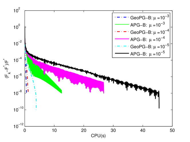
(a) Dataset a9a

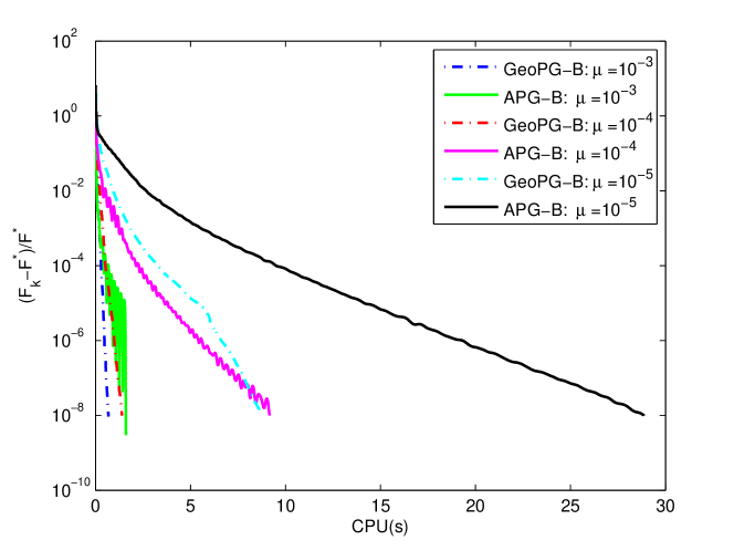
(b) Dataset RCV1

Figure 1: GeoPG-B and APG-B for solving (C.1) with $\alpha=10^{-8}$.

5.2 Logistic regression with elastic net regularization

In this subsection, we compare the performance of GeoPG-B and APG-B for solving the following logistic regression problem with elastic net regularization:

$$\min_{x\in\mathbb{R}^{n}}\ \frac{1}{p}\sum_{i=1}^{p}\log\big{(}1+\exp(-b_{i}\cdot a_{i}^{\top}x)\big{)}+\frac{\alpha}{2}\|x\|^{2}+\mu\|x\|_{1},$$ (5.2)

where $a_{i}\in\mathbb{R}^{n}$ and $b_{i}\in\{\pm 1\}$ are the feature vector and class label of the $i$-th sample, respectively, and $\alpha$, $\mu>0$ are the weighting parameters.

We tested GeoPG-B and APG-B for solving (C.2) on the three real datasets a9a, RCV1 and Gisette from LIBSVM, and the results are reported in Figure 2. In particular, we tested $\alpha=10^{-8}$ and $\mu=10^{-3},10^{-4},10^{-5}$. Figure 2 shows that for the same $\mu$, GeoPG-B is much faster than APG-B. More numerical results are provided in the appendix, which also indicate that GeoPG-B is much faster than APG-B, especially when the problems are more ill-conditioned.

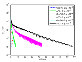
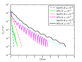
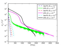
Figure 2: GeoPG-B and APG-B for solving (C.2) with $\alpha=10^{-8}$. Left: dataset a9a; Middle: dataset RCV1; Right: dataset Gisette.

5.3 Numerical results of L-GeoPG-B

In this subsection, we test GeoPG with limited memory described in Algorithm 5 for solving (C.2) on the Gisette dataset. Since we still need to use the backtracking technique, we actually tested L-GeoPG-B. The results with different memory sizes $m$ are reported in Figure 3. Note that $m=0$ corresponds to the original GeoPG-B without memory. The subproblem (4.4) is solved using the function “quadprog” in Matlab. From Figure 3 we see that roughly speaking, L-GeoPG-B performs better for larger memory sizes, and in most cases, the performance of L-GeoPG-B with $m=100$ is the best among the reported results. This indicates that the limited-memory idea indeed helps improve the performance of GeoPG.

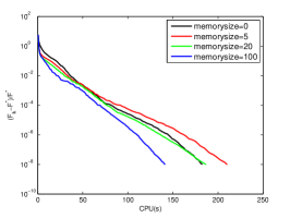
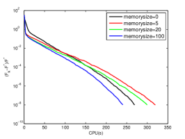
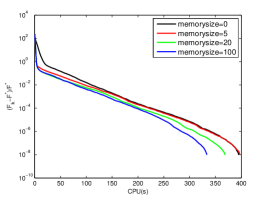
Figure 3: L-GeoPG-B for solving (C.2) on the dataset Gisette with $\alpha=10^{-8}$. Left: $\lambda=10^{-3}$; Middle: $\lambda=10^{-4}$; Right: $\lambda=10^{-5}$.

6 Conclusions

In this paper, we proposed a GeoPG algorithm for solving nonsmooth convex composite problems, which is an extension of the recent method GeoD that can only handle smooth problems. We proved that GeoPG enjoys the same optimal rate as Nesterov’s accelerated gradient method for solving strongly convex problems. The backtracking technique was adopted to deal with the case when the Lipschitz constant is unknown. Limited-memory GeoPG was also developed to improve the practical performance of GeoPG. Numerical results on linear regression and logistic regression with elastic net regularization demonstrated the efficiency of GeoPG. It would be interesting to see how to extend GeoD and GeoPG to tackle non-strongly convex problems, and how to further accelerate the running time of GeoPG. We leave these questions in future work.

Appendix

Appendix A Geometric Interpretation of GeoPG

We argue that the geometric intuition of GeoPG is still clear. Note that we are still constructing two balls that contain $x^{*}$ and shrink at the same absolute amount. In GeoPG, since we assume that the smooth function $f$ is strongly convex, we naturally have one ball that contains $x^{*}$, and this ball is related to the proximal gradient $G_{t}$, instead of the gradient due to the presence of the nonsmooth function $h$. To construct the other ball, GeoD needs to perform an exact line search, while our GeoPG needs to find the root of a newly constructed function $\bar{\phi}$, which is again due to the presence of the nonsmooth function $h$. The two changes of GeoPG from GeoD are: replace gradient by proximal gradient; replace the exact line search by finding the root of $\bar{\phi}$, both of which are resulted by the presence of the nonsmooth function $h$.

Appendix B Proofs

B.1 Proof of Lemma 3.1

Proof.

From the $\beta$-smoothness of $f$, we have

$$f(x^{+})\leq f(x)-t\langle\nabla f(x),G_{t}(x)\rangle+\frac{t}{2}\|G_{t}(x)\|^{2}.$$ (B.1)

Combining (B.1) with

$$f(x)+\langle\nabla f(x),y-x\rangle+\frac{\alpha}{2}\|y-x\|^{2}\leq f(y),\ \forall x,y\in\mathbb{R}^{n},$$ (B.2)

yields that

$$F(x^{+}) \leq f(y)-\langle\nabla f(x),y-x\rangle-\frac{\alpha}{2}\|y-x\|^{2}-t\langle\nabla f(x),G_{t}(x)\rangle+\frac{t}{2}\|G_{t}(x)\|^{2}+h(x^{+})$$ (B.3)

$$=F(y)-\frac{\alpha}{2}\|y-x\|^{2}+\frac{t}{2}\|G_{t}(x)\|^{2}+h(x^{+})-h(y)-\langle\nabla f(x)-G_{t}(x),y-x^{+}\rangle-\langle G_{t}(x),y-x^{+}\rangle$$

$$\leq F(y)-\frac{\alpha}{2}\|y-x\|^{2}+\frac{t}{2}\|G_{t}(x)\|^{2}-\langle G_{t}(x),y-x^{+}\rangle,$$

where the last inequality is due to the convexity of $h$ and $G_{t}(x)\in\nabla f(x)+\partial h(x^{+})$. ∎

B.2 Proof of Lemma 3.2

Proof.

Assume

$$\langle x_{k}^{+}-x_{k},x_{k-1}^{+}-x_{k}\rangle\leq 0,\mbox{ and }\langle x_{k}^{+}-x_{k},x_{k}-c_{k-1}\rangle\geq 0,$$ (B.4)

holds. By letting $y=x_{k-1}^{+}$ and $x=x_{k}$ in (B.3), we have

$$F(x_{k}^{+}) \leq F(x_{k-1}^{+})-\langle G_{t}(x_{k}),x_{k-1}^{+}-x_{k}\rangle-\frac{t}{2}\|G_{t}(x_{k})\|^{2}-\frac{\alpha}{2}\|x_{k-1}^{+}-x_{k}\|^{2}$$

$$=F(x_{k-1}^{+})+\frac{1}{t}\langle x_{k}^{+}-x_{k},x_{k-1}^{+}-x_{k}\rangle-\frac{t}{2}\|G_{t}(x_{k})\|^{2}-\frac{\alpha}{2}\|x_{k-1}^{+}-x_{k}\|^{2}$$

$$\leq F(x_{k-1}^{+})-\frac{t}{2}\|G_{t}(x_{k})\|^{2},$$

where the last inequality is due to (B.4). Moreover, from the definition of $x_{k}^{++}$ and (B.4) it is easy to see

$$\|x_{k}^{++}-c_{k-1}\|^{2} =\|x_{k}-c_{k-1}\|^{2}+\frac{2}{\alpha t}\langle x_{k}^{+}-x_{k},x_{k}-c_{k-1}\rangle+\frac{1}{\alpha^{2}}\|G_{t}(x_{k})\|^{2}\geq\frac{1}{\alpha^{2}}\|G_{t}(x_{k})\|^{2}.$$

∎

B.3 Proof of Lemma 3.3

Before we prove Lemma 3.3, we need the following well-know result, which can be found in [21].

Lemma. (see Lemma 3.9 of [21]) For $t\in(0,1/\beta]$, $G_{t}(x)$ is strongly monotone, i.e.,

$$\langle G_{t}(x)-G_{t}(y),x-y\rangle\geq\frac{\alpha}{2}\|x-y\|^{2},\forall x,y.$$ (B.5)

We are now ready to prove Lemma 3.3.

Proof.

We prove (i) first.

$$|\phi_{t,x,c}(z_{1})-\phi_{t,x,c}(z_{2})| =|\langle z_{1}^{+}-z_{1}-(z_{2}^{+}-z_{2}),x-c\rangle|\leq\|z_{1}^{+}-z_{2}^{+}-(z_{1}-z_{2})\|\|x-c\|$$

$$\leq(\|\text{prox}_{th}(z_{1}-t\nabla f(z_{1}))-\text{prox}_{th}(z_{2}-t\nabla f(z_{2}))\|+\|z_{1}-z_{2}\|)\|x-c\|$$

$$\leq(2+t\beta)\|x-c\|\|z_{1}-z_{2}\|,$$

where the last inequality is due to the non-expansiveness of the proximal mapping operation.

We now prove (ii). For $s_{1}<s_{2}$, let $z_{1}=x+s_{1}(c-x)$ and $z_{2}=x+s_{2}(c-x)$. We have

$$\bar{\phi}_{t,x,c}(s_{2})-\bar{\phi}_{t,x,c}(s_{1}) =\langle z_{2}^{+}-z_{2}-(z_{1}^{+}-z_{1}),x-c\rangle=\frac{t}{s_{2}-s_{1}}\langle G_{t}(z_{2})-G_{t}(z_{1}),z_{2}-z_{1}\rangle$$

$$\geq\frac{\alpha t}{2}(s_{2}-s_{1})\|x-c\|^{2}>0,$$

where the first inequality follows from (B.5). ∎

Appendix C Numerical Experiment on Other Datasets

In this section, we report some numerical results of other data sets. Here we set the terminate condition as $\|G_{t}(x_{k}^{+})\|_{\infty}\leq tol$ for GeoP-B and $\|G_{t}(x_{k})\|_{\infty}\leq tol$ for APG-B.

C.1 Linear regression with elastic net regularization

In this subsection, we compare GeoPG-B and APG-B for solving linear regression with elastic net regularization:

$$\min_{x\in\mathbb{R}^{n}}\ \frac{1}{2p}\|Ax-b\|^{2}+\frac{\alpha}{2}\|x\|^{2}+\mu\|x\|_{1},$$ (C.1)

where $A\in\mathbb{R}^{p\times n}$, $b\in\mathbb{R}^{p}$, $\alpha,\mu>0$ are weighting parameters.

We first compare these two algorithms on some synthetic data. In our experiments, entries of $A$ were drawn randomly from the standard Gaussian distribution, the solution $\bar{x}$ was a sparse vector with 10% nonzero entries whose locations are uniformly random and whose values follow the Gaussian distribution $3*\mathcal{N}(0,1)$, and $b=A*\bar{x}+\mathbf{n}$, where the noise $\mathbf{n}$ follows the Gaussian distribution $0.01*\mathcal{N}(0,1)$. Moreover, since we assume that the strong convexity parameter of (C.1) is equal to $\alpha$, when $p>n$, we manipulate $A$ such that the smallest eigenvalue of $A^{\top}A$ is equal to 0. Specifically, when $p>n$, we truncate the smallest eigenvalue of $A^{\top}A$ to 0, and obtain the new $A$ by eigenvalue decomposition of $A^{\top}A$. We set $tol=10^{-8}$.

In Tables 1, 2 and 3, we report the comparison results of GeoPG-B and APG-B for solving different instances of (C.1). We use “f-ev”, “g-ev”, “p-ev” and “MVM” to denote the number of evaluations of objective function, gradient, proximal mapping of $\ell_{1}$ norm, and matrix-vector multiplications, respectively. The CPU times are in seconds. We use “–” to denote that the algorithm does not converge in $10^{5}$ iterations. We tested different values of $\alpha$, which reflect different condition numbers of the problem. We also tested different values of $\mu$, which was set to $\mu=(10^{-3},10^{-4},10^{-5})/p\times\|A^{\top}b\|_{\infty}$, respectively. “f-diff” denotes the absolute difference of the objective values returned by the two algorithms.

From Tables 1, 2 and 3 we see that GeoPG-B is more efficient than APG-B in terms of CPU time when $\alpha$ is small. For example, Table 1 indicates that GeoPG-B is faster than APG-B when $\alpha\leq 10^{-4}$, Table 2 indicates that GeoPG-B is faster than APG-B when $\alpha\leq 10^{-6}$, and Table 3 shows that GeoPG-B is faster than APG-B when $\alpha\leq 10^{-8}$. Since a small $\alpha$ corresponds to a large condition number, we can conclude that in this case GeoPG-B is more preferable than APG-B for ill-conditioned problems. Note that “f-diff” is very small in all cases, which indicates that the solutions returned by GeoPG-B and APG-B are very close.

We also conducted tests on three real datasets downloaded from the LIBSVM repository: a9a, RCV1 and Gisette, among which a9a and RCV1 are sparse and Gisette is dense. The size and sparsity (percentage of nonzero entries) of these three datasets are $(32561\times 123,11.28\%)$, $(20242\times 47236,0.16\%)$ and $(6000\times 5000,99.1\%)$, respectively. The results are reported in Tables 4, 5 and 6, where $\alpha=10^{-2},10^{-4},10^{-6},10^{-8},10^{-10}$ and $\mu=10^{-3},10^{-4},10^{-5}$. We see from these tables that GeoPG-B is faster than APG-B on these real datasets when $\alpha$ is small, i.e., when the problem is more ill-conditioned.

C.2 Logistic regression with elastic net regularization

In this subsection, we compare the performance of GeoPG-B and APG-B for solving the following logistic regression problem with elastic net regularization:

$$\min_{x\in\mathbb{R}^{n}}\ \frac{1}{p}\sum_{i=1}^{p}\log(1+\exp(-b_{i}\cdot a_{i}^{\top}x))+\frac{\alpha}{2}\|x\|^{2}+\mu\|x\|_{1},$$ (C.2)

where $a_{i}\in\mathbb{R}^{n}$ and $b_{i}\in\{\pm 1\}$ are the feature vector and class label of the $i$-th sample, respectively, and $\alpha$, $\mu>0$ are weighting parameters.

We first compare GeoPG-B and APG-B for solving (C.2) on some synthetic data. In our experiments, each $a_{i}$ was drawn randomly from the standard Gaussian distribution, the linear model parameter $\bar{x}$ was a sparse vector with 10% nonzero entries whose locations are uniformly random and whose values follow the Gaussian distribution $3*\mathcal{N}(0,1)$, and $\ell=A*\bar{x}+\mathbf{n}$, where noise $\mathbf{n}$ follows the Gaussian distribution $0.01*\mathcal{N}(0,1)$. Then, we generate class labels as bernoulli random variables with the parameter $1/(1+\exp{\ell_{i}})$. We set $tol=10^{-8}$.

In Tables 7, 8 and 9 we report the comparison results of GeoPG-B and APG-B for solving different instances of (C.2). From results in these tables we again observe that GeoPG-B is faster than APG-B when $\alpha$ is small, i.e., when the condition number is large.

We also tested GeoPG-B and APG-B for solving (C.2) on the three real datasets a9a, RCV1 and Gisette from LIBSVM, and the results are reported in Tables 10, 11 and 12. We again have the similar observations as before, i.e., GeoPG-B is faster than APG-B for more ill-conditioned problems.

C.3 More discussions on the numerical results

To the best of our knowledge, the FISTA algorithm [15] does not have a counterpart for strongly convex problem, but we still conducted some numerical experiments using FISTA for solving the above problems. We found that FISTA and APG are comparable, but they are both worse than GeoPG for more ill-conditioned problems. Moreover, from the results in this section, we can see that when the problem is well-posed such as $\alpha=0.01$, APG is usually faster than GeoPG in the CPU time, and when the problem is ill-posed such as $\alpha=10^{-6}$, $10^{-8}$, $10^{-10}$, GeoPG is usually faster, but the iterate of GeoPG is less than APG in the most cases. So GeoPG is not always better than APG in the CPU time. But since ill-posed problems are more challenging to solve, we believe that these numerical results showed the potential of GeoPG. The reason why GeoPG is better than APG for ill-posed problem is still not clear at this moment, but we think that it might be related to the fact that APG is not monotone but GeoPG is, which can be seen from the figures in our paper. Furthermore, although GeoPG requires to find the root of a function $\bar{\phi}$ in each iteration, we found that a very good approximation of the root can be obtained by running the semi-smooth Newton method for 1-2 iterations on average. This explains why these steps of GeoPG do not bring much trouble in practice.

C.4 Numerical results of L-GeoPG-B

In this subsection, we tested GeoPG-B with limited memory described in Algorithm 5 on solving (C.2) on Gisette dataset. The results for different memory size $m$ are reported in Table 13. Note that $m=0$ corresponds to the original GeoPG-B without memory.

From Table 13 we see that roughly speaking, L-GeoPG-B performs better for larger memory size, and in almost all cases, the performance of L-GeoPG-B with $m=100$ is the best among the reported results. This indicates that the limited-memory idea indeed helps improve the performance of GeoPG.

Table 1: GeoPG-B and APG-B for solving linear regression with elastic net regularization. $p=4000,n=2000$

	APG-B						GeoPG-B
$\alpha$	iter	cpu	f-ev	g-ev	p-ev	MVM	iter	cpu	f-ev	g-ev	p-ev	MVM	f-diff
$\mu=1.136e-02$
$10^{-2}$	172	1.0	354	326	194	384	156	1.1	457	348	352	398	8.5e-14
$10^{-4}$	538	2.8	1116	1020	611	1203	95	0.7	267	240	245	247	6.4e-14
$10^{-6}$	905	4.9	1868	1715	1029	2030	94	0.7	260	249	254	247	5.0e-14
$10^{-8}$	1040	5.4	2146	2003	1182	2332	95	0.7	263	258	263	247	1.4e-14
$10^{-10}$	964	5.0	2002	1805	1095	2154	95	0.7	263	267	272	247	2.1e-14
$\mu=1.136e-03$
$10^{-2}$	175	0.9	356	332	197	392	168	1.2	493	384	388	432	1.3e-13
$10^{-4}$	687	3.6	1414	1304	779	1539	145	1.0	411	392	397	377	1.5e-14
$10^{-6}$	999	5.1	2086	1676	1134	2225	140	1.0	371	384	394	354	6.5e-14
$10^{-8}$	1122	5.8	2348	1827	1275	2499	143	1.0	374	420	429	365	1.8e-15
$10^{-10}$	1142	5.9	2388	1858	1298	2545	143	1.0	374	449	458	365	6.2e-15
$\mu=1.136e-04$
$10^{-2}$	168	0.9	346	314	189	374	113	0.8	328	252	256	296	1.4e-14
$10^{-4}$	911	4.8	1836	1853	1035	2064	207	1.5	603	587	592	535	4.1e-14
$10^{-6}$	2293	11.9	4744	3936	2605	5132	191	1.4	523	596	602	492	3.8e-14
$10^{-8}$	3979	20.5	8266	5923	4526	8899	199	1.4	500	713	728	501	9.8e-14
$10^{-10}$	4503	23.3	9364	6668	5123	10068	185	1.3	456	624	639	465	5.9e-14

Table 2: GeoPG-B and APG-B for solving linear regression with elastic net regularization. $p=2000,n=2000$

	APG-B						GeoPG-B
$\alpha$	iter	cpu	f-ev	g-ev	p-ev	MVM	iter	cpu	f-ev	g-ev	p-ev	MVM	f-diff
$\mu=1.50e-02$
$10^{-2}$	244	0.7	498	475	276	548	304	1.3	889	690	694	774	3.4e-13
$10^{-4}$	1800	4.8	3690	3582	2046	4048	545	2.4	1569	1298	1308	1378	1.3e-12
$10^{-6}$	9706	26.0	19722	20445	11040	21926	557	2.3	1598	1328	1339	1415	2.8e-12
$10^{-8}$	20056	53.7	40528	43361	22817	45427	561	2.3	1614	1332	1344	1416	2.4e-12
$10^{-10}$	20473	53.9	41426	44159	23298	46357	565	2.3	1626	1373	1385	1436	2.4e-12
$\mu=1.50e-03$
$10^{-2}$	241	0.6	496	463	273	540	280	1.2	813	634	638	716	1.4e-14
$10^{-4}$	1926	5.1	3968	3708	2188	4319	1218	5.0	3560	2875	2892	3073	2.0e-11
$10^{-6}$	12502	32.7	25658	24681	14222	28118	1297	5.3	3718	3065	3097	3262	1.1e-11
$10^{-8}$	47139	124.3	95560	100584	53646	106652	1289	5.3	3686	3043	3074	3245	2.1e-11
$10^{-10}$	72186	194.3	145934	156713	82157	163534	1297	5.2	3717	3098	3132	3262	2.5e-11
$\mu=1.50e-04$
$10^{-2}$	239	0.6	488	460	270	536	225	0.9	648	510	514	584	3.3e-13
$10^{-4}$	1985	5.2	4048	3860	2257	4476	1713	6.9	5041	4040	4058	4322	7.0e-11
$10^{-6}$	13824	35.7	28534	25354	15726	31010	2527	10.2	7225	6019	6082	6345	2.5e-11
$10^{-8}$	56339	146.2	116280	106460	64105	126410	2594	10.6	7288	6095	6182	6491	3.6e-11
$10^{-10}$	$-$	$-$	$-$	$-$	$-$	$-$	2573	10.4	7217	6075	6163	6446	$-$

Table 3: GeoPG-B and APG-B for solving linear regression with elastic net regularization. $p=2000,n=4000$

	APG-B						GeoPG-B
$\alpha$	iter	cpu	f-ev	g-ev	p-ev	MVM	iter	cpu	f-ev	g-ev	p-ev	MVM	f-diff
$\mu=1.82e-02$
$10^{-2}$	327	1.9	660	680	371	740	387	2.8	1117	936	946	980	2.0e-13
$10^{-4}$	2263	12.8	4620	4445	2571	5096	2454	17.9	6858	6181	6225	6168	4.3e-11
$10^{-6}$	12579	67.5	25566	26229	14312	28421	4478	32.7	12494	11180	11216	11300	1.8e-11
$10^{-8}$	55577	299.3	112140	121939	63268	126044	4595	33.7	12814	11754	11795	11609	1.4e-10
$10^{-10}$	$-$	$-$	$-$	$-$	$-$	$-$	4645	34.6	13204	12088	12129	11729	$-$
$\mu=1.82e-03$
$10^{-2}$	306	1.7	622	621	346	688	279	2.1	813	677	684	713	6.4e-13
$10^{-4}$	2355	12.7	4820	4534	2675	5296	2634	19.3	7482	6774	6846	6596	3.9e-13
$10^{-6}$	14827	79.8	30328	28671	16862	33388	12756	94.1	36510	32580	32735	32121	2.2e-10
$10^{-8}$	56286	305.7	114576	115199	64050	127099	11665	88.0	32397	32580	31987	29352	6.1e-11
$10^{-10}$	$-$	$-$	$-$	$-$	$-$	$-$	13830	102.4	38547	37931	38088	34885	$-$
$\mu=1.82e-04$
$10^{-2}$	283	1.5	576	560	320	636	219	1.6	643	523	528	561	4.7e-13
$10^{-4}$	2420	13.2	4864	5242	2749	5487	2339	17.2	6818	6467	6509	5882	5.8e-11
$10^{-6}$	16882	91.4	34412	31337	19186	38049	14803	109.3	41943	44052	44384	37152	4.9e-10
$10^{-8}$	79693	430.5	163098	146951	90639	179423	41331	305.8	116983	113344	113952	104206	1.6e-10
$10^{-10}$	$-$	$-$	$-$	$-$	$-$	$-$	47501	350.2	129513	151332	152224	119660	$-$

Table 4: GeoPG-B and APG-B for solving linear regression with elastic net regularization on dataset a9a

	APG-B						GeoPG-B
$\alpha$	iter	cpu	f-ev	g-ev	p-ev	MVM	iter	cpu	f-ev	g-ev	p-ev	MVM	f-diff
$\lambda=1e-03$
$10^{-2}$	266	0.3	540	530	301	599	260	0.6	769	602	608	662	1.3e-14
$10^{-4}$	1758	1.7	3562	3683	1998	3974	463	1.1	1374	1138	1144	1196	1.2e-14
$10^{-6}$	10790	10.4	21654	23858	12277	24518	410	0.9	1216	964	970	1058	1.5e-13
$10^{-8}$	23279	22.2	46646	52163	26493	52943	412	0.9	1222	976	982	1060	1.9e-13
$10^{-10}$	26057	24.9	52236	58464	29660	59260	431	0.9	1279	1063	1069	1104	2.2e-13
$\lambda=1e-04$
$10^{-2}$	267	0.3	544	526	302	600	249	0.5	734	571	577	642	6.7e-16
$10^{-4}$	1948	1.9	3934	4100	2214	4410	1587	3.4	4747	3946	3951	4025	2.9e-12
$10^{-6}$	14954	14.3	30012	33215	17018	33985	4801	10.4	14388	11381	11386	12223	1.4e-12
$10^{-8}$	63920	60.9	127954	144494	72741	145426	910	2.0	2715	2629	2634	2347	3.7e-12
$10^{-10}$	94861	90.6	189814	214931	107970	215895	910	2.0	2715	2441	2446	2333	7.0e-13
$\lambda=1e-05$
$10^{-2}$	258	0.3	518	507	292	584	235	0.5	692	596	602	604	1.2e-14
$10^{-4}$	2035	1.9	4088	4319	2315	4622	1701	3.7	5090	4267	4273	4312	3.7e-12
$10^{-6}$	16353	15.6	32768	36396	18609	37188	5773	12.5	17306	14961	14967	14808	4.5e-13
$10^{-8}$	85246	81.4	170570	193007	97062	194086	2109	4.6	6314	6403	6409	5382	2.5e-11
$10^{-10}$	$-$	$-$	$-$	$-$	$-$	$-$	2318	5.0	6941	6709	6715	5896	$-$

Table 5: GeoPG-B and APG-B for solving linear regression with elastic net regularization on dataset rcv1

	APG-B						GeoProx-B
$\alpha$	iter	cpu	f-ev	g-ev	p-ev	MVM	f-diff	cpu	f-ev	g-ev	p-ev	MVM	f-diff
$\lambda=1e-03$
$10^{-2}$	18	0.1	34	34	20	42	14	0.2	39	31	32	43	5.5e-14
$10^{-4}$	74	0.3	148	141	82	165	95	0.7	273	231	232	245	7.8e-13
$10^{-6}$	329	1.5	678	617	372	735	103	0.8	296	265	268	269	6.6e-13
$10^{-8}$	908	4.2	1872	1721	1033	2039	133	1.0	380	344	345	341	7.0e-13
$10^{-10}$	1277	5.9	2630	2482	1454	2871	116	0.9	332	331	332	301	1.1e-12
$\lambda=1e-04$
$10^{-2}$	17	0.1	32	31	19	40	17	0.1	48	34	35	49	1.6e-13
$10^{-4}$	109	0.5	226	195	123	243	109	0.5	226	195	123	243	1.7e-12
$10^{-6}$	723	3.2	1482	1401	821	1625	251	1.9	743	625	633	634	1.3e-11
$10^{-8}$	3087	13.9	6276	6426	3513	6976	247	2.1	723	645	653	626	1.4e-11
$10^{-10}$	5266	23.7	10638	11244	5991	11930	244	1.9	711	672	678	624	6.0e-12
$\lambda=1e-05$
$10^{-2}$	16	0.1	30	28	18	38	15	0.1	42	32	33	45	3.1e-13
$10^{-4}$	118	0.5	240	220	134	267	125	1.0	359	289	294	321	1.0e-10
$10^{-6}$	859	3.9	1750	1595	978	1941	833	6.8	2470	2186	2199	2105	5.7e-10
$10^{-8}$	5902	26.5	11918	11933	6716	13376	1179	9.6	3509	3336	3348	2998	1.4e-09
$10^{-10}$	33127	150.7	66438	72792	37722	75353	1180	9.7	3508	3540	3555	2995	7.2e-10

Table 6: GeoPG-B and APG-B for solving linear regression with elastic net regularization on data set Gisette. Note that neither APG-B nor GeoPG-B converges in $10^{5}$ iterations when $\mu=1e-05$ and $\alpha=10^{-6},10^{-8},10^{-10}$.

	APG-B						GeoPG-B
$\alpha$	iter	cpu	f-ev	g-ev	p-ev	MVM	iter	cpu	f-ev	g-ev	p-ev	MVM	f-diff
$\mu=1e-03$
$10^{-2}$	4026	198.1	8144	7729	4583	9121	4253	239.3	12593	10474	10506	10758	4.8e-14
$10^{-4}$	30537	1504.2	61478	61380	34786	69371	6030	342.4	17939	17977	18006	15411	1.6e-13
$10^{-6}$	$-$	$-$	$-$	$-$	$-$	$-$	5197	294.0	15419	16126	16159	13241	$-$
$10^{-8}$	$-$	$-$	$-$	$-$	$-$	$-$	5692	322.8	16950	18851	18881	14506	$-$
$10^{-10}$	$-$	$-$	$-$	$-$	$-$	$-$	6150	353.5	18295	23420	23450	15714	$-$
$\mu=1e-04$
$10^{-2}$	6084	299.5	12288	12211	6930	13801	5406	304.3	16046	13623	13658	13675	1.1e-13
$10^{-4}$	49467	2434.4	99880	100633	56333	112194	36606	2046.7	105023	112545	113414	91853	1.6e-13
$10^{-6}$	$-$	$-$	$-$	$-$	$-$	$-$	20821	1179.7	62243	65886	65919	53105	$-$
$10^{-8}$	$-$	$-$	$-$	$-$	$-$	$-$	21575	1224.1	64488	71718	71753	54979	$-$
$10^{-10}$	$-$	$-$	$-$	$-$	$-$	$-$	20328	1164.9	60730	76896	76942	51908	$-$
$\mu=1e-05$
$10^{-2}$	6570	323.9	13304	13289	7483	14885	4803	270.8	14228	11515	11547	12164	2.7e-13
$10^{-4}$	56562	2791.0	114250	115944	64396	128230	38001	2153.4	113603	100036	100105	96725	5.6e-12

Table 7: GeoPG-B and APG-B for solving logistic regression with elastic net regularization. $p=6000,n=3000$

	APG-B						GeoPG-B
$\alpha$	iter	cpu	f-ev	g-ev	p-ev	MVM	iter	cpu	f-ev	g-ev	p-ev	MVM	f-diff
$\mu=1.00e-03$
$10^{-2}$	55	0.9	112	96	60	158	46	1.3	125	145	146	207	1.1e-13
$10^{-4}$	256	4.3	536	470	289	761	55	1.7	144	194	194	269	5.6e-13
$10^{-6}$	509	8.7	1048	972	577	1551	61	2.0	164	218	220	300	1.3e-12
$10^{-8}$	573	9.5	1188	1086	649	1737	60	1.9	161	223	225	305	1.4e-12
$10^{-10}$	585	9.6	1208	1112	663	1777	59	2.1	158	231	233	313	1.4e-12
$\mu=1.00e-04$
$10^{-2}$	51	0.7	104	80	55	137	51	1.3	141	167	164	236	2.5e-13
$10^{-4}$	203	3.0	422	336	226	564	118	3.2	319	405	396	555	1.3e-11
$10^{-6}$	954	14.7	1994	1662	1080	2744	126	3.8	335	452	450	614	3.1e-11
$10^{-8}$	1814	28.7	3780	3311	2056	5369	125	3.7	336	454	454	614	2.6e-11
$10^{-10}$	2135	33.9	4444	3952	2421	6375	125	4.0	336	475	475	635	3.2e-11
$\mu=1.00e-05$
$10^{-2}$	52	0.8	102	88	57	147	40	1.0	107	129	128	184	2.3e-13
$10^{-4}$	141	1.9	288	208	154	364	97	2.4	257	316	309	438	3.3e-11
$10^{-6}$	576	7.8	1246	804	646	1452	139	4.0	350	496	488	669	5.6e-11
$10^{-8}$	2797	38.4	6070	4014	3166	7182	148	4.4	372	538	535	723	4.0e-10
$10^{-10}$	4549	63.3	9862	6703	5151	11856	153	4.9	392	585	583	776	6.2e-10

Table 8: GeoPG-B and APG-B for solving logistic regression with elastic net regularization. $p=3000,n=6000$

	APG-B						GeoPG-B
$\alpha$	iter	cpu	f-ev	g-ev	p-ev	MVM	iter	cpu	f-ev	g-ev	p-ev	MVM	f-diff
$\mu=1.00e-03$
$10^{-2}$	58	0.9	114	107	63	172	60	1.6	169	200	196	279	5.1e-14
$10^{-4}$	253	4.1	516	466	284	752	110	3.5	292	420	412	562	1.9e-12
$10^{-6}$	893	15.1	1824	1757	1012	2771	115	4.3	305	467	463	615	4.1e-12
$10^{-8}$	1265	21.9	2584	2543	1435	3980	114	4.4	302	504	501	649	4.9e-12
$10^{-10}$	1333	22.6	2712	2691	1513	4206	114	4.8	302	543	540	688	5.0e-12
$\mu=1.00e-04$
$10^{-2}$	56	0.8	112	89	60	151	42	1.1	116	133	132	188	1.4e-13
$10^{-4}$	159	2.2	328	237	174	413	128	3.7	340	455	447	616	1.7e-11
$10^{-6}$	750	11.3	1560	1238	845	2085	157	5.2	392	621	614	817	5.3e-11
$10^{-8}$	1927	30.3	4012	3447	2182	5631	158	5.8	410	679	674	877	8.6e-11
$10^{-10}$	2364	37.5	4934	4290	2677	6969	164	6.6	427	760	753	965	1.5e-10
$\mu=1.00e-05$
$10^{-2}$	54	0.8	108	85	58	145	42	1.1	110	136	134	191	2.9e-13
$10^{-4}$	118	1.6	236	177	126	305	81	2.1	207	266	263	365	1.4e-11
$10^{-6}$	493	6.4	1062	636	551	1189	153	4.9	365	588	580	776	2.9e-10
$10^{-8}$	3492	45.0	7742	4365	3949	8316	163	5.8	379	686	677	886	8.3e-10
$10^{-10}$	7655	98.4	17058	9498	8666	18166	169	6.8	403	782	775	990	1.7e-09

Table 9: GeoPG-B and APG-B for solving logistic regression with elastic net regularization. $p=3000,n=3000$

	APG-B						GeoPG-B
$\alpha$	iter	cpu	f-ev	g-ev	p-ev	MVM	iter	cpu	f-ev	g-ev	p-ev	MVM	f-diff
$\mu=1.00e-03$
$10^{-2}$	55	0.5	110	99	60	161	53	0.8	144	172	171	243	2.7e-13
$10^{-4}$	278	2.4	566	512	312	826	90	1.4	237	325	322	442	2.7e-12
$10^{-6}$	845	7.1	1732	1637	957	2596	89	1.5	234	336	334	452	2.6e-12
$10^{-8}$	1158	9.7	2378	2283	1314	3599	89	1.6	234	361	359	477	2.6e-12
$10^{-10}$	1186	9.9	2444	2340	1345	3687	88	1.7	231	377	375	492	2.8e-12
$\mu=1.00e-04$
$10^{-2}$	55	0.4	108	89	60	151	53	0.7	144	172	169	242	3.5e-13
$10^{-4}$	172	1.3	352	273	191	466	122	1.8	327	424	415	579	3.2e-11
$10^{-6}$	868	6.6	1834	1455	980	2437	145	2.3	374	529	523	714	6.8e-11
$10^{-8}$	1985	16.0	4168	3527	2248	5777	144	2.5	372	565	563	747	5.9e-11
$10^{-10}$	2475	19.9	5160	4545	2807	7354	143	2.7	365	607	605	787	7.4e-11
$\mu=1.00e-05$
$10^{-2}$	55	0.4	108	91	59	152	48	0.7	129	158	155	224	6.7e-13
$10^{-4}$	126	0.9	256	185	137	324	126	0.9	256	185	137	324	2.0e-12
$10^{-6}$	515	3.4	1108	680	576	1258	146	2.2	344	524	517	705	4.6e-10
$10^{-8}$	3196	21.0	7054	4118	3615	7735	154	2.5	372	587	586	778	8.9e-10
$10^{-10}$	6434	42.7	14228	8384	7284	15670	152	2.8	370	630	629	820	5.4e-10

Table 10: GeoPG-B and APG-B for solving logistic regression with elastic net on dataset a9a

	APG-B						GeoPG-B
$\alpha$	iter	cpu	f-ev	g-ev	p-ev	MVM	iter	cpu	f-ev	g-ev	p-ev	MVM	f-diff
$\mu=1.00e-03$
$10^{-2}$	99	0.3	196	189	111	302	96	0.5	280	325	318	450	2.9e-15
$10^{-4}$	676	1.8	1380	1317	766	2085	676	1.8	1380	1317	766	2085	1.7e-14
$10^{-6}$	2696	6.8	5484	5466	3065	8533	187	1.0	540	663	683	885	2.6e-14
$10^{-8}$	3911	9.8	7934	8114	4445	12561	188	1.0	545	654	678	876	2.0e-14
$10^{-10}$	4324	10.9	8770	9013	4917	13932	200	1.1	581	758	783	991	5.9e-14
$\mu=1.00e-04$
$10^{-2}$	96	0.2	194	174	106	282	96	0.2	194	174	106	282	1.1e-14
$10^{-4}$	709	1.7	1440	1388	805	2195	756	3.8	2251	2669	2577	3615	8.2e-13
$10^{-6}$	5195	13.6	10488	10973	5912	16887	2581	13.4	7725	8995	8770	12112	4.4e-11
$10^{-8}$	25300	64.8	50772	56141	28793	84936	716	3.7	2130	2529	2583	3427	9.9e-10
$10^{-10}$	42633	109.4	85446	95447	48519	143968	723	3.8	2151	2584	2640	3497	7.9e-11
$\mu=1.00e-05$
$10^{-2}$	106	0.3	210	199	119	320	72	0.4	207	258	255	347	1.4e-14
$10^{-4}$	770	1.9	1550	1526	874	2402	685	3.5	2038	2448	2367	3301	3.7e-12
$10^{-6}$	5842	14.7	11762	12434	6648	19084	3026	15.5	9061	11099	10715	14750	2.1e-11
$10^{-8}$	46819	119.9	93782	104946	53311	158259	7784	38.8	23335	26969	26326	36558	1.9e-12
$10^{-10}$	$-$	$-$	$-$	$-$	$-$	$-$	1488	8.2	4447	5674	5721	7567	$-$

Table 11: GeoPG-B and APG-B for solving logistic regression with elastic net on dataset RCV1

	APG-B						GeoPG-B
$\alpha$	iter	cpu	f-ev	g-ev	p-ev	MVM	iter	cpu	f-ev	g-ev	p-ev	MVM	f-diff
$\mu=1e-03$
$10^{-2}$	15	0.1	28	26	17	45	7	0.1	21	22	23	36	5.0e-14
$10^{-4}$	35	0.2	68	61	37	100	30	0.3	83	91	93	134	7.7e-13
$10^{-6}$	112	0.7	224	213	125	340	43	0.5	120	136	140	193	1.3e-12
$10^{-8}$	196	1.2	390	384	220	606	39	0.5	110	137	138	191	4.3e-12
$10^{-10}$	230	1.4	466	444	259	705	39	0.5	110	149	150	203	1.3e-12
$\mu=1e-04$
$10^{-2}$	13	0.1	24	22	15	39	11	0.1	32	35	36	56	3.0e-13
$10^{-4}$	40	0.3	80	75	44	121	42	0.5	122	136	135	193	3.8e-12
$10^{-6}$	178	1.0	368	311	200	513	153	1.8	431	542	527	738	6.2e-11
$10^{-8}$	1039	6.2	2122	1941	1179	3122	137	1.6	384	495	503	673	1.9e-11
$10^{-10}$	1983	11.7	4080	3724	2251	5977	137	1.7	379	526	524	705	2.5e-12
$\mu=1e-05$
$10^{-2}$	13	0.1	24	22	15	39	9	0.1	26	28	29	45	2.3e-13
$10^{-4}$	42	0.2	84	71	46	119	39	0.4	108	120	122	173	2.3e-11
$10^{-6}$	164	0.9	338	266	182	450	208	2.5	592	747	729	1012	1.4e-09
$10^{-8}$	1115	6.4	2274	2013	1266	3281	377	4.7	1073	1436	1410	1901	5.5e-09
$10^{-10}$	5569	33.5	11314	11135	6334	17471	486	6.2	1399	1930	1897	2542	6.5e-10

Table 12: GeoPG-B and APG-B for solving logistic regression with elastic net on dataset Gisette

	APG-B						GeoPG-B
$\alpha$	iter	cpu	f-ev	g-ev	p-ev	MVM	iter	cpu	f-ev	g-ev	p-ev	MVM	f-diff
$\mu=1e-03$
$10^{-2}$	630	40.4	1267	1176	717	1895	819	82.5	2298	2867	2790	3903	2.8e-14
$10^{-4}$	2445	156.0	4923	4511	2784	7297	2177	217.5	6197	7710	7477	10406	3.9e-13
$10^{-6}$	13950	915.2	28209	28106	15889	43997	2013	230.9	5654	7676	7737	10200	2.0e-12
$10^{-8}$	64288	4397.1	129271	140483	73191	213676	1793	214.9	5033	7146	7188	9371	4.4e-14
$10^{-10}$	$-$	$-$	$-$	$-$	$-$	$-$	1808	227.1	5079	7532	7559	9783	$-$
$\mu=1e-04$
$10^{-2}$	913	57.7	1845	1744	1041	2787	961	93.7	2740	3335	3237	4553	3.5e-13
$10^{-4}$	1889	113.1	3811	3246	2150	5398	913	57.7	1845	1744	1041	2787	3.9e-12
$10^{-6}$	10206	614.4	20687	17730	11632	29364	2243	258.2	6044	8768	8763	11486	3.0e-11
$10^{-8}$	53272	3405.7	107397	103641	60702	164345	2226	276.7	6001	9318	9300	12002	2.8e-11
$10^{-10}$	$-$	$-$	$-$	$-$	$-$	$-$	2203	296.2	5926	9809	9812	12488	$-$
$\mu=1e-05$
$10^{-2}$	975	63.2	1981	1882	1110	2994	795	79.8	2242	2738	2662	3747	6.5e-13
$10^{-4}$	1485	91.1	3019	2632	1687	4321	1381	141.4	3760	4943	4829	6686	6.8e-12
$10^{-6}$	4642	265.8	9439	7240	5286	12528	2928	313.0	7964	10940	10698	14554	1.5e-11
$10^{-8}$	29242	1681.8	59811	46411	33325	79738	2946	374.2	7789	12617	12543	16128	5.5e-10
$10^{-10}$	$-$	$-$	$-$	$-$	$-$	$-$	2776	436.6	7359	13607	13563	16936	$-$

Table 13: L-GeoPG-B for solving logistic regression with elastic net regularization on data set Gisette

	$m=0$		$m=5$		$m=10$		$m=20$		$m=50$		$m=100$
$\alpha$	iter	cpu	iter	cpu	iter	cpu	iter	cpu	iter	cpu	iter	cpu
$\mu=1e-03$
$10^{-2}$	819	82.5	1310	164.1	1015	125.8	902	97.0	713	76.6	769	93.6
$10^{-4}$	2177	217.5	3656	470.8	3439	417.9	3836	406.6	2399	260.1	1530	185.8
$10^{-6}$	2013	230.9	1606	235.9	1589	221.5	1547	225.4	1344	189.6	1082	168.4
$10^{-8}$	1793	214.9	1622	252.7	1530	224.4	1562	234.6	1363	200.8	1097	172.7
$10^{-10}$	1808	227.1	1599	260.8	1549	245.3	1565	246.9	1369	216.9	1100	180.8
$\mu=1e-04$
$10^{-2}$	961	93.7	2573	312.6	2057	251.5	1487	169.6	1367	137.8	1217	130.0
$10^{-4}$	2146	217.2	2237	312.3	2595	341.6	2621	314.0	2044	242.8	1317	179.6
$10^{-6}$	2243	258.2	2102	307.0	2105	303.9	1979	292.2	1810	272.3	1390	219.9
$10^{-8}$	2226	276.7	2057	329.4	2009	317.6	1951	313.6	1791	288.1	1444	250.5
$10^{-10}$	2203	296.2	2046	361.7	2101	342.1	2002	338.3	1846	307.6	1445	246.7
$\mu=1e-05$
$10^{-2}$	795	79.8	3501	407.2	3022	359.3	1375	166.75	1156	122.7	968	106.7
$10^{-4}$	1381	141.4	1461	219.2	1303	179.2	1621	213.7	1198	153.5	902	126.6
$10^{-6}$	2928	313.0	2343	352.7	2271	336.2	2179	323.8	2001	297.6	1601	256.3
$10^{-8}$	2946	374.2	2401	380.0	2349	380.5	2254	360.8	2099	345.6	1804	303.9
$10^{-10}$	2776	436.7	2503	432.4	2363	414.3	2350	409.4	2093	365.7	1826	320.2

References

- Bubeck et al. [2015] S. Bubeck, Y.-T. Lee, and M. Singh. A geometric alternative to Nesterov’s accelerated gradient descent. arXiv preprint arXiv:1506.08187, 2015.
- Nesterov [1983] Y. E. Nesterov. A method for unconstrained convex minimization problem with the rate of convergence . Dokl. Akad. Nauk SSSR, 269:543–547, 1983.
- Nesterov [2004] Y. E. Nesterov. Introductory lectures on convex optimization: A basic course. Applied Optimization. Kluwer Academic Publishers, Boston, MA, 2004. ISBN 1-4020-7553-7.
- Su et al. [2014] W. Su, S. Boyd, and E. J. Candès. A differential equation for modeling Nesterov’s accelerated gradient method: Theory and insights. In NIPS, 2014.
- Attouch et al. [2016] H. Attouch, Z. Chbani, J. Peypouquet, and P. Redont. Fast convergence of inertial dynamics and algorithms with asymptotic vanishing viscosity. Mathematical Programming, 2016.
- Lessard et al. [2016] L. Lessard, B. Recht, and A. Packard. Analysis and design of optimization algorithms via integral quadratic constraints. SIAM Journal on Optimization, 26(1):57–95, 2016.
- Wibisono et al. [2016] A. Wibisono, A. Wilson, and M. I. Jordan. A variational perspective on accelerated methods in optimization. Proceedings of the National Academy of Sciences, 133:E7351–E7358, 2016.
- Bland et al. [1981] R. G. Bland, D. Goldfarb, and M. J. Todd. The ellipsoid method: A survey. Operations Research, 29:1039–1091, 1981.
- Bubeck and Lee [2016] S. Bubeck and Y.-T. Lee. Black-box optimization with a politician. ICML, 2016.
- Drusvyatskiy et al. [2016] D. Drusvyatskiy, M. Fazel, and S. Roy. An optimal first order method based on optimal quadratic averaging. SIAM Journal on Optimization, 2016.
- Brent [1973] R. P. Brent. An algorithm with guaranteed convergence for finding a zero of a function. In Algorithms for Minimization without Derivatives. Englewood Cliffs, NJ: Prentice-Hall, 1973.
- Dekker [1969] T. J. Dekker. Finding a zero by means of successive linear interpolation. In Constructive Aspects of the Fundamental Theorem of Algebra. London: Wiley-Interscience, 1969.
- Gerdts et al. [2017] M. Gerdts, S. Horn, and S. Kimmerle. Line search globalization of a semismooth Newton method for operator equations in Hilbert spaces with applications in optimal control. Journal of Industrial And Management Optimization, 13(1):47–62, 2017.
- Hans and Raasch [2015] E. Hans and T. Raasch. Global convergence of damped semismooth Newton methods for L1 Tikhonov regularization. Inverse Problems, 31(2):025005, 2015.
- Beck and Teboulle [2009] A. Beck and M. Teboulle. A fast iterative shrinkage-thresholding algorithm for linear inverse problems. SIAM J. Imaging Sciences, 2(1):183–202, 2009.
- Scheinberg et al. [2014] K. Scheinberg, D. Goldfarb, and X. Bai. Fast first-order methods for composite convex optimization with backtracking. Foundations of Computational Mathematics, 14(3):389–417, 2014.
- Nesterov [2013] Y. E. Nesterov. Gradient methods for minimizing composite functions. Mathematical Programming, 140(1):125–161, 2013.
- Beck [2007] A. Beck. On the convexity of a class of quadratic mappings and its application to the problem of finding the smallest ball enclosing a given intersection of balls. Journal of Global Optimization, 39(1):113–126, 2007.
- Eldar et al. [2008] Y. C. Eldar, A. Beck, and M. Teboulle. A minimax Chebyshev estimator for bounded error estimation. IEEE Transactions on Signal Processing, 56(4):1388–1397, 2008.
- Zou and Hastie [2005] H. Zou and T. Hastie. Regularization and variable selection via the elastic net. Journal of the Royal Statistical Society, Series B, 67(2):301–320, 2005.
- Lee et al. [2014] J. D. Lee, Y. Sun, and M. A. Saunders. Proximal Newton-type methods for minimizing composite functions. SIAM Journal on Optimization, 24(3):1420–1443, 2014.