Molecular nucleation theory of dust formation in core-collapse supernovae applied to SN 1987A

Abstract

We model dust formation in the core collapse supernova explosion SN 1987A by treating the gas-phase formation of dust grain nuclei as a chemical process. To compute the synthesis of fourteen species of grains we integrate a non-equilibrium network of nucleating and related chemical reactions and follow the growth of the nuclei into grains via accretion and coagulation. The effects of the radioactive ⁵⁶Co, ⁵⁷Co, ⁴⁴Ti, and ²²Na on the thermodynamics and chemistry of the ejecta are taken into account. The grain temperature, which we allow to differ from the gas temperature, affects the surface-tension-corrected evaporation rate. We also account for He⁺, Ne⁺, Ar⁺, and O weathering. We combine our dust synthesis model with a crude prescription for anisotropic ⁵⁶Ni dredge-up into the core ejecta, the so-called “nickel bubbles”, to compute the total dust mass and molecular-species-specific grain size distribution. The total mass varies between $0.41\,M_{\odot}$ and $0.73\,M_{\odot}$, depending on the bubble shell density contrast. In the decreasing order of abundance, the grain species produced are: magnesia, silicon, forsterite, iron sulfide, carbon, silicon dioxide, alumina, and iron. The combined grain size distribution is a power law $dN/da\propto a^{-4.39}$. Early ejecta compaction by expanding radioactive ⁵⁶Ni bubbles strongly enhances dust synthesis. This underscores the need for improved understanding of hydrodynamic transport and mixing over the entire pre-homologous expansion.

1 Introduction

Dust grains are important throughout astrophysics. They absorb ultraviolet (UV) and visible light and radiate in the infrared (IR). This produces the extinction and reddening (Mathis, 1990) that must be taken into account when inferring the properties of astronomical sources such as the star formation rates of galaxies (Kennicutt, 1998; Calzetti et al., 2000; Dunne et al., 2011). Dust grains are a component of the interstellar medium (ISM) that is essential to the star formation process (Draine, 2003; McKee & Ostriker, 2007; Draine, 2011; Kennicutt & Evans, 2012). They shield the interiors of dense molecular clouds from molecule-dissociating radiation. They act as cooling agents in star-forming gas clouds and as catalysts for formation of the molecules, such as H₂, that do not form efficiently in the gas phase (Cazaux & Tielens, 2002). Grains are also essential in planet formation (Williams & Cieza, 2011). Since grains are composed of refractory elements such as carbon, oxygen, and silicon, these elements are depleted from the gas phase. In the densest, coldest molecular gas, volatile compounds such as H₂O and CO₂ form icy mantles on refractory grain cores. Radiation pressure on grains can drive winds from cool, evolved stars and potentially also drive outflows in active galactic nuclei and starbursts.

Given the ubiquity and importance of dust grains in the cosmos, it is vital that we understand how they are produced, modified, and destroyed. In principle, dust grains can form in any environment where an initially hot, dense gas expands and cools, as in explosions and outflows, or where a gas cloud is being compressed isothermally to high densities, as in pre-stellar cores. Decades of research, however, point to the stellar winds from the cool atmospheres of asymptotic giant branch and supergiant stars (e.g., Ferrarotti & Gail, 2006) and the expanding ejecta of supernovae (e.g., Clayton et al., 1997; Derdzinski et al., 2017) as the main contributors of dust. Interstellar dust grains may also form in novae (e.g., Mitchell & Evans, 1984; Rawlings & Williams, 1989), in outflows from active galactic nuclei (e.g., Elvis et al., 2002), in the material ejected in stellar mergers and common envelope systems (e.g., Lü et al., 2013), in the colliding winds of Wolf-Rayet stars (e.g., Crowther, 2003), and in extreme mass loss events in luminous blue variables (e.g., Kochanek, 2011). It is unknown exactly what fraction of dust mass comes from each of these classes of events. The origin of this uncertainty seems to be an incomplete theoretical understanding of the astrophysics of dust formation.

Dust formation can be directly observed in nearby core-collapse supernovae through the dust’s imprint on supernova spectra (Sugerman et al., 2006; Fox et al., 2009, 2010; Kotak et al., 2009; Sakon et al., 2009; Inserra et al., 2011; Meikle et al., 2011; Szalai et al., 2011; Maeda et al., 2013). As dust grains condense in supernova ejecta, the spectrum of the supernova changes in three characteristic ways. The optical luminosity of the ejecta decreases due to absorption by grains. The IR luminosity increases as the grains reradiate the absorbed energy in the IR while the total luminosity of the ejecta decreases following the progression of radioactive decay. The peaks of optical emission lines are blueshifted as optical photons from the far side of the ejecta are more likely to be absorbed (e.g., Smith et al., 2012).

Due to its proximity, SN 1987A in the Large Magellanic Cloud has been the best studied case of dust formation in supernovae (e.g., Gehrz & Ney, 1987, 1990; Dwek, 1988; Kozasa et al., 1989; Kozasa et al., 1991; Moseley et al., 1989; McCray, 1993; Colgan et al., 1994; Ercolano et al., 2007; Van Dyk, 2013; Indebetouw et al., 2014; Matsuura et al., 2015; Wesson et al., 2015). Wesson et al. (2015) used three-dimensional radiation transfer calculations to simulate the evolution of the spectral energy distribution (SED) of SN 1987A while varying the dust mass, grain chemical composition, grain size distribution, and location of dust in the ejecta. They are able to reproduce the observed SEDs if: (1) dust mass increases from $0.001\,M_{\odot}$ at 615 days to $0.8\,M_{\odot}$ at 9200 days after the explosion, (2) while the dust mass always increases, most of the dust forms well after 1000 days, (3) the dust is mostly carbon with some silicates (perhaps 85% carbon and 15% silicates), (4) the grain radius distribution has a logarithmic slope of $-3.5$ but the typical grain radius increases from $\approx 0.04\,\mu\text{m}$ at 615 days after the explosion to $3\,\mu\text{m}$ at 9200 days, (5) dust forms in clumps that occupy $\sim 10\%$ of the volume of the ejecta and have clump radii $\sim 1/30$ of the ejecta radius (so there are $\approx 2700$ clumps), and (6) the clumps expand sub-homologously. Bevan & Barlow (2016) have confirmed these relatively large dust masses by modeling the observed emission line profiles with Monte Carlo radiation transfer calculations. In contrast, Dwek & Arendt (2015) infer a sharply different, early and rapid dust mass evolution. By 615 days, the dust mass has already reached $0.45\,M_{\odot}$, with $0.4\,M_{\odot}$ in silicates and $0.05\,M_{\odot}$ in amorphous carbon, and that over the following two decades, the dust mass does not increase appreciably. In this work we attempt to shed light on this apparent disagreement.

There are a few other supernovae that have shown evidence of dust formation, mostly through blueshifted emission lines (Milisavljevic et al., 2012). However, due to the large distances, it is typically difficult to observe the signatures of dust formation. Alternatively, one can search for evidence of dust in supernova remnants in the Milky Way and its satellite galaxies (e.g., Sandstrom et al., 2009; Rho et al., 2009). Probably the most studied such object is Cassiopeia A, the remnant of a supernova at a distance of $\sim 3.5\,\text{kpc}$ that was observed to explode about 300 years ago (see, e.g., Dunne et al., 2009). Detecting alumina, carbon, enstatite, forsterite, magnesium protosilicates, silicon dioxide, silicon, iron, iron oxide, and iron sulfide with the Spitzer Space Telescope spectroscopy, Rho et al. (2008) showed that $0.02-0.054\,M_{\odot}$ of dust has formed in its ejecta. De Looze et al. (2017) used spatially resolved Herschel and Spitzer observations of Cas A to infer a cold dust mass of $0.1\,M_{\odot}<M_{\rm dust}<0.6\,M_{\odot}$ in the unshocked ejecta. Bevan et al. (2017) used the damocles Monte Carlo radiation transfer code and observations of the blueshifted emission lines in the spectrum of SN 1980K, SN 1993J, and Cas A to infer a dust mass of $0.12\,M_{\odot}<M_{\rm dust}<0.3\,M_{\odot}$ in SN 1980K, $0.08\,M_{\odot}<M_{\rm dust}<0.1\,M_{\odot}$ in SN 1993J, and $M_{\rm dust}\approx 1.1M_{\odot}$ in Cas A. A significant dust mass has also been detected in the Crab nebula (Gomez et al., 2012; Owen & Barlow, 2015). Its IR spectrum can be fitted with a dust size distribution that is a power law with slope between $-3.5$ and $-4$ (Temim & Dwek, 2013).

Supernovae provide unique physical conditions for the production of dust grains. While the average metal mass fraction in galaxies is of the order of 1%, supernova ejecta can be 100% metal. The ejecta is exposed to the $\gamma$ rays, X-rays, and nonthermal electrons and positrons produced in the radioactive decay of ⁵⁶Co, ⁵⁷Co, ⁴⁴Ti, and ²²Na. These nonthermal particles ionize atoms and dissociate molecules and thus modify the chemistry of the ejecta. For example, destruction of molecules can liberate metals to become incorporated in grains, whereas ionization of noble gas atoms provides agents for grain weathering.

The grains produced in the ejecta must ultimately survive destruction in the reverse shock before becoming a part of the ISM (e.g., Biscaro & Cherchneff, 2016; Micelotta et al., 2016). How much of the dust made in a supernova makes it to the ISM depends strongly on the grain size distribution, with larger grains in denser clumps more likely to survive the reverse shock (e.g., Bianchi & Schneider, 2007; Nozawa et al., 2007, 2010; Bocchio et al., 2016). After newly formed grains enter the ISM, they are modified by shock waves created by supernovae, by coagulation, by cosmic ray sputtering, and by accretion of gas phase metals (and volatiles such as H₂O and CO). Grains can also be destroyed if they become incorporated in stars.

The dust grains’ effects depend on the chemical composition and size. These properties should not be spatially uniform in the ISM because grains form in some environments and are modified in others. For example, extinction curve variation shows that that grains in dense molecular cloud cores have different properties than those in the diffuse ISM (Chapman et al., 2009). In an attempt to model the grain properties, theoretical computations of dust grain formation have been attempted at various levels of physical realism, each one adding a formidable layer of complexity. Specifically, in the 30 years since SN1987A, three significantly different approaches to simulating dust formation in supernovae have emerged.

The simplest approach is the classical nucleation theory (CNT) that treats grain formation as a barrier-crossing problem in which the free energy of a small cluster of atoms first increases as atoms are added to the cluster. When a critical cluster size is reached, the free energy then begins to decrease as further atoms are added. The CNT provides the rate per unit volume, called the nucleation current, at which critical-size clusters come into existence, as well as the rate at which the nucleated clusters grow into grains by accreting gas-phase atoms. To estimate the nucleation current, the CNT assumes that a steady state has been attained between monomer attachment and detachment. The CNT ignores the actual chemical reactions participating in the formation of the cluster. It assumes that clusters have thermodynamic properties of the bulk material from which they are made and are subject to surface tension. It ignores chemical reactions that can destroy grains and ignores grain growth by coagulation. Thanks to its simplicity, the CNT has been widely used, for example by Kozasa et al. (1989); Kozasa et al. (1991) in the modeling of dust grain formation in SN 1987A. Todini & Ferrara (2001) used the CNT to model dust formation in core collapse supernovae from Population III star progenitors and Schneider et al. (2004) for dust formation in pair-instability supernovae (also from Population III stellar progenitors). Bianchi & Schneider (2007) used it to calculate the amount of dust produced in a SN 1987A-like explosion. Recently, Marassi et al. (2015) used it on a grid of progenitor and explosion models to compute the properties of grains formed in Population III supernovae.

The second method of modeling dust formation in supernovae is kinetic nucleation theory (KNT). In the KNT, the number densities $c_{n}$ of clusters of $n\geq 2$ atoms (called $n$-mers) are explicitly tracked. Grains are allowed to grow by addition of atoms (condensation) and erode by removal of atoms (evaporation). The condensation rate is computed from kinetic theory and the evaporation rate by applying the principle of detailed balance. The KNT is more realistic than the CNT in that it does not assume a steady state between condensation and evaporation. However it still ignores the actual chemical reactions participating in the formation of the initial seed nucleus of a dust grain. In modeling the evaporation rate, it assumes that the grains has thermodynamic properties of a solid bulk material with surface tension correction. It ignores chemical reactions contributing to grain destruction and also ignores grain growth by coagulation. The elements of this technique can be found in Nozawa et al. (2003) and Nozawa & Kozasa (2013). Nozawa et al. (2008) used the KNT to model dust formation in SN 2006jc and Lazzati & Heger (2016) for the formation of carbon grains in core-collapse supernova ejecta.

The third approach to modeling dust formation, one that we will adopt, could be called ‘molecular nucleation theory’ (MNT). It explicitly tracks the abundance of each molecular species (such as CO and SiO) with a non-equilibrium chemical reaction network. Specifically, it follows the chemical binding of clusters of monomers such as C₄ or Mg₄Si₂O₈ into larger $n$-mers that are still treated as molecular entities. The molecules that have reached a certain size can then act as grain condensation and coagulation nuclei. MNT was introduced in Cherchneff & Lilly (2008) that investigated molecular synthesis in a pair-instability-type Population III supernova. Cherchneff & Dwek (2009) included the effects of radioactivity and Cherchneff & Dwek (2010) further computed the formation of condensation nuclei for various types of dust grains in both pair instability and core collapse supernovae. Sarangi & Cherchneff (2013) extended this framework to cluster nucleation in Type II-P supernovae. These applications of MNT did not treat dust grain growth, but only the formation of the molecular and cluster precursors that is the first stage of dust grain formation. Sarangi & Cherchneff (2015) extended MNT to the grains themselves and began estimating the grain size distribution and total dust mass yield for various grain types.

The cited studies of dust formation in supernovae assumed that supernova ejecta were either fully mixed (single zone models) or spherically symmetric (one-dimensional models). In one-dimensional models the ejecta are divided into concentric shells, each characterized by an initial elemental composition and prescribed thermal evolution. The shells at smaller radial mass coordinates contain heavier elements and expand from higher initial densities and temperatures. Recent realistic three-dimensional simulations of supernovae, however, suggest that the ejecta are not spherically symmetric (Hammer et al., 2010; Wongwathanarat et al., 2010). Heavy elements such as ⁵⁶Ni can be ejected ahead of lighter elements such as ¹²C (Wongwathanarat et al., 2013, 2015; Wongwathanarat et al., 2017). This anisotropy is a consequence of the amplification of non-spherical perturbations by the Rayleigh-Taylor instability (also called Ritchmyer-Meshkov instability in impulsively accelerated fluid). Sources of initial perturbations are turbulence and convection during the unstable, dynamical inner-shell (e.g., silicon) burning in the progenitor (Arnett & Meakin, 2011; Ono et al., 2013; Smith & Arnett, 2014; Couch et al., 2015; Müller et al., 2016) as well as neutrino-induced convection behind the stalled shock wave and the standing accretion shock instability (e.g., Hanke et al., 2013; Abdikamalov et al., 2015; Lentz et al., 2015, and references therein). Perturbations are amplified into nonlinear fingers in compositional interfaces where the mean molecular mass and the density drop sharply outward (e.g., Mao et al., 2015; Wongwathanarat et al., 2015). The interfaces are unstable because in the aftermath of the shock crossing, they are where the acceleration vector (relative a local freely falling frame) aligns with a strong density gradient, both pointing inward.

A consequence of the strongly-aspherical explosion geometry is that blobs of the ⁵⁶Ni synthesized during $\alpha$-rich freezeout of complete explosive silicon burning are ejected into, and become embedded within, lighter-element material. The ⁵⁶Ni decays into ⁵⁶Co which then decays into ⁵⁶Fe. These radioactive decays deposit thermal energy in the gas. The heating raises the pressure in the blobs above the pressure in the surrounding ejecta. The overpressured ⁵⁶Ni-enriched blobs are termed “bubbles” (e.g., Fryxell et al., 1991; Herant et al., 1992). The bubbles expand super-homologously with respect to the rest of the ejecta. The expanding bubbles can sweep up thin, high density shells. Once the bubbles and their shells become optically thin to the $\gamma$ rays emitted during radioactive decay, their interior pressure drops and they resume homologous expansion (Wang, 2005). The shell surrounding a bubble may itself become Rayleigh-Taylor unstable and fragment (Basko, 1994). Once molecules and dust grains form in the shell, the shell may cool so rapidly that its pressure drops below that of the ambient ejecta. In this case, the shell can enter contraction (in homologously expanding coordinates).

This basic “bubbly" structure is in fact observed in young supernova remnants such as the Cas A (Milisavljevic & Fesen, 2015) and also the remnant B0049-73.6 in the Small Magellanic Cloud (Hendrick et al., 2005). Recently, Abellán et al. (2017) used observations with the Atacama Large Millimeter/submillimeter Array (ALMA) to create three dimensional maps of CO and SiO in the inner ejecta of SN 1987A. These maps definitively show that the distribution of molecules is not uniform but clumpy in the inner ejecta. Matsuura et al. (2017) used ALMA observations at high frequency resolution to detect CO, SiO, SO, and HCO⁺ in the ejecta of SN1987A. The distorted profiles of the emission lines from these molecules also imply that they are not uniformly distributed in the ejecta.

Quantity	Symbol	Unit
bulk binding energy of atom to grain divided by Boltzmann’s constant	$A$	K
Hamaker constant	$A_{\rm H}$	erg
Arrhenius rate coefficient	$A_{j}$	$\text{cm}^{\{0,3,6\}}\,\text{s}^{-1}\,\text{molecule}^{-1}$
radius of monomer	$a_{1}$	cm
radius of $n$-mer	$a_{n}$	cm
grain radius	$a$	cm
maximum grain radius	$a_{\rm max}$	cm
minimum grain radius	$a_{\rm min}$	cm
$\ell$th grain radius grid point	$a_{\ell}$	cm
number of times that species $i$ occurs as a product in reaction $j$	$\alpha_{ij}$
parameter in vapor pressure approximation formula	$B$
number of times that species $i$ occurs as a reactant in reaction $j$	$\beta_{ij}$
Coulomb correction factor	$\mathcal{C}_{\ell_{1}\ell_{2}}$
number density of molecules of species $i$	$c_{i}$	$\text{cm}^{-3}$
number density of electrons	$c_{e}$	$\text{cm}^{-3}$
number density of ions	$c_{\rm ion}$	$\text{cm}^{-3}$
number density of monomers	$c_{1}$	$\text{cm}^{-3}$
number density of $n$-mers	$c_{n}$	$\text{cm}^{-3}$
number density of grains at radius grind point $\ell$	$c_{\ell}$	$\text{cm}^{-3}$
number density of the key species	$c_{\rm key}$	$\text{cm}^{-3}$
total gas number density	$c_{\rm tot}$	$\text{cm}^{-3}$
surface binding energy of an atom to a grain	$\mathcal{E}_{\rm bind}$	erg
activation energy	$E_{\rm A,\it j}$	erg
energy emitted in X-rays, electrons, and positrons in one decay of isotope $n$	$E_{n}^{\rm X}$	keV
energy emitted in $\gamma$-rays in one decay of isotope $n$	$E_{n}^{\gamma}$	MeV
number of vibrational degrees of freedom in a grain	$F$
fraction of deposited radioactive energy that goes into ionizing and dissociating atoms and molecules	$f_{\rm ion}$
fraction of deposited radioactive energy that goes into UV photons	$f_{\rm UV}$
calibration ratio of gas temperature used in simulation to temperature from cloudy	$f_{\rm temp}$
rate at which electrons collide with a grain	$\Gamma_{e^{-}}$	$\text{s}^{-1}\,\text{grain}^{-1}$
rate at which electrons are ejected from a grain following absorption of a photon	$\Gamma_{\gamma}$	$\text{s}^{-1}\,\text{grain}^{-1}$
rate at which ions collide with a grain	$\Gamma_{\rm ion}$	$\text{s}^{-1}\,\text{grain}^{-1}$
average number of quanta per vibrational degree of freedom	$\gamma$
coagulation kernel	$K_{\ell_{1}\ell_{2}}$	$\text{cm}^{3}\,\text{s}^{-1}$
accretion rate coefficient	$k_{\rm acc}$	$\text{cm}^{3}\,\text{s}^{-1}$
evaporation rate in monomers ejected per unit time per grain	$k_{\rm evap}$	$\text{s}^{-1}$
rate coefficient for reaction $j$	$k_{j}$	$\text{cm}^{\{0,3,6\}}\,\text{s}^{-1}$
rate coefficient for Compton destruction of species $i$ via process $j$	$k_{i,j}^{\rm C}$	$\text{s}^{-1}$
rate coefficient for noble gas ion weathering	$k_{\rm He}$	$\text{cm}^{3}\,\text{s}^{-1}$
rate coefficient for oxygen weathering	$k_{\rm O}$	$\text{cm}^{3}\,\text{s}^{-1}$
rate at which energy from all decaying isotopes is deposited in the ejecta	$L$	$\text{erg}\,\text{s}^{-1}$
rate at which a grain absorbs energy from the UV radiation field	$L_{\rm abs}$	$\text{erg}\,\text{s}^{-1}$
rate at which a grain emits energy in the form of thermal radiation	$L_{\rm emit}$	$\text{erg}\,\text{s}^{-1}$
rate at which energy is transferred from the gas to a grain	$L_{\rm gas}$	$\text{erg}\,\text{s}^{-1}$
rate at which energy is deposited in the ejecta that destroys atoms and molecules	$L_{\rm ion}$
rate at which energy from decaying isotope $n$ is deposited in the ejecta	$L_{n}$	$\text{erg}\,\text{s}^{-1}$
rate at which energy is converted into UV radiation in the ejecta	$L_{\rm UV}$	$\text{erg}\,\text{s}^{-1}$
number of radius bins	$\ell_{\rm max}$
decay rate of isotope $n$	$\lambda_{n}$	$\text{yr}^{-1}$
mass coordinate in ejecta	$M$	$M_{\odot}$
total dust mass produced in simulation	$M_{\rm dust,tot}$	$M_{\odot}$
total dust mass in SN 1987A as a function of time	$M_{\rm dust,tot,1987A}$	$M_{\odot}$
enclosed mass coordinate in the mesa model	$M_{\text{ej},\textsc{mesa}}$	$M_{\odot}$
mass of ejected helium and metal core in SN 1987A	$M_{\rm ej,tot,1987A}$	$M_{\odot}$
mass of ejected helium and metal core in the mesa model	$M_{\text{ej,tot},\textsc{mesa}}$	$M_{\odot}$
mean molecular weight	$\left\langle m\right\rangle$	g
mass of monomer	$m_{1}$	g
mass of $n$-mer	$m_{n}$	g
mass of ions	$m_{\rm ion}$	g
molecular mass of the key species	$m_{\rm key}$	g
mass of grain at grid point $\ell$	$m_{\ell}$	g
reduced mass of colliding grains	$\mu_{\ell_{1}\ell_{2}}$	g
reduced mass	$\mu$	g

Table 1: Index of notation used in the paper.

Quantity	Symbol	Unit
total number of dependent variables in the system of ODEs that we are solving	$\mathcal{N}$
number of grain species	$\mathcal{N}_{\rm G}$
number of radioactive isotopes	$\mathcal{N}_{\rm iso}$
number of reactions	$\mathcal{N}_{\rm R}$
number of species (of molecules) in simulation	$\mathcal{N}_{\rm S}$
number of atoms in a grain	$N$
number of atoms of isotope $n$ in ejecta	$N_{n}$
total number of particles in the ejecta	$N_{\rm tot}$
number of monomers	$n$
number density of UV photons per unit photon energy	$n_{\gamma}$	$\text{cm}^{-3}\,\text{eV}^{-1}$
number of monomers in a grain at grid point $\ell$	$n_{\ell}$
number of monomers that you have to add to $\mathcal{Z}_{\ell-1}$ to obtain $\mathcal{Z}_{\ell}$	$\delta n_{\ell-1}$
number of monomers in largest cluster	$n_{\rm max}$
power law exponent in Arrhenius form of rate coefficient	$\nu_{j}$
the $k$th stoichiometric coefficient in the formula for accretion/evaporation	$\nu_{k}$
stoichiometric coefficient of the key species	$\nu_{\rm key}$
angular frequency of vibrational degrees of freedom in a grain	$\omega_{0}$	$\text{rad}\,\text{s}^{-1}$
standard pressure	$p_{\rm s}$	$\text{dyne}\,\text{cm}^{-2}$
absorption coefficient	$Q_{\rm abs}$
radius of the outer edge of core ejecta	$R$	cm
mass density of ejecta	$\rho$	$\text{g}\,\text{cm}^{-3}$
ejecta mass density at reference time $t_{0}$	$\rho_{0}$	$\text{g}\,\text{cm}^{-3}$
mass density of grain	$\varrho$	$\text{g}\,\text{cm}^{-3}$
evaporation suppression factor	$S_{N}$
sticking coefficient	$s_{n}$
collision cross section	$\sigma$	$\text{cm}^{2}$
surface tension	$\sigma_{\text{ST}}$	$\text{erg}\,\text{cm}^{-2}$
photon absorption cross section	$\sigma_{\rm abs}$	$\text{cm}^{2}$
temperature	$T$	K
activation energy divided by Boltzmann’s constant	$T_{\rm A,\it j}$	K
Debye temperature	$T_{\rm D}$	K
grain temperature	$T_{\rm dust}$	K
electron temperature	$T_{e}$	K
gas temperature	$T_{\rm gas}$	K
temperature of ions	$T_{\rm ion}$	K
time since explosion	$t$	s
reference time	$t_{0}$	$=100\,\text{d}$
optical depth of ejecta	$\tau$
optical depth of ejecta to $\gamma$ photons emitted by isotope $n$	$\tau_{n}$
thermal energy in a grain	$U$	erg
total energy in UV radiation field	$U_{\rm UV}$	erg
energy density in UV radiation field	$u_{\rm UV}$	$\text{erg}\,\text{cm}^{-3}$
potential energy due to van der Waals forces	$V_{\ell_{1}\ell_{2}}$	erg
amount of energy that an electron loses when it destroys a molecule of species $i$ via process $j$	$W_{i}^{j}$	eV
van der Waals correction factor	$\mathcal{W}_{\ell_{1}\ell_{2}}$
monomer of a single element grain	$\mathcal{X}$
$n$-mer	$\mathcal{X}_{n}$
condensation nucleus	$\mathcal{X}_{n_{\rm max}}$
mass fraction of isotope $i$	$X_{i}$
photoelectric yield	$Y$
grain at radial grid point $\ell$	$\mathcal{Z}_{\ell}$
grain that results from coagulation of grains in bin $i$ and $j$	$\mathcal{Z}_{\ell_{1}\ell_{2}}$
equilibrium grain charge	$Z_{\rm dust}$	$e$
grain charge	$Z$	$e$
charge of grain at radial grid point $\ell$ in units of $e$	$Z_{\ell}$	$e$
charge of ions	$z_{\rm ion}$	$e$

Table 2: Index of notation used in the paper (continued).

Here we present a model of dust formation in supernovae constructed within the framework of MNT. We precompute initial data for local temperature and mass density evolution of the ejecta and for the local nucleosynthetic yields and then follow the formation of molecules with a fully nonequilibrium chemical reaction network. The model includes reactions such as: three-body molecular association, thermal fragmentation, neutral-neutral and ion-molecule reactions, radiative association, charge exchange, recombination with electrons in the gas-phase, and destruction by energetic electrons produced by the radioactive decay of ⁵⁶Co, ⁵⁷Co, ⁴⁴Na, and ⁴⁴Ti. The formation of large molecules that act as condensation nuclei for grains is followed as part of this network. The grains grow by accreting gas-phase molecules and coagulating. The coagulation rate accounts for the effects of the van der Waals force and also the Coulomb force due to grain electric charge. Grains lose mass through evaporation, reaction with noble gas ions, and oxidation. The grain temperature, which is needed for the evaporation rate, is allowed to differ from the gas temperature and depend on the grain radius and post-explosion epoch. The evaporation rate computation includes the effects of surface tension and the lack of gas-grain thermal coupling (the latter implying that the thermodynamic fluctuation leading to evaporation must come from within the grain itself). We consider several representative ejecta fluid elements, each of which has its own chemical composition and thermodynamic evolution, and track molecule and grain formation in each element. Our simulation calculates the abundance of each species (atoms, molecules, ions, free electrons, and dust condensation nuclei) as a function of time from the explosion. The calculation provides us with the properties of dust formed in each representative fluid element.

The paper is organized as follows. In Section 2 we present our modeling of the radioactive heat and ionization sources in the ejecta and of the structure and thermal evolution of the ejecta. In Section 3 we describe our chemical framework and in Section 4 we describe our modeling of grain growth and destruction processes. In Section 5 we describe our time integration scheme. In Section 6 we present the results and in Section 7 we discuss the implications of our results and delineate desirable next steps. Finally, in Section 8 we summarize our main conclusions. In Tables 1–2 we provide overview of the important mathematical notation used in the paper.

2 Supernova model

2.1 Radioactive decay

Explosive nucleosynthesis produces large quantities of radioactive nuclei and their decay has profound consequences for the thermal and chemical evolution of the ejecta. Let $N_{n}(0)$ be the total number of atoms of radioactive isotope $n$ immediately after the explosion. Then at time $t$ after the explosion, the remaining number of atoms of the radioactive isotope is $N_{n}(t)=N_{n}(0)e^{-\lambda_{n}t}$, where $\lambda_{n}$ is the decay rate. The number of decays per unit time is $|dN_{n}/dt|=\lambda_{n}N_{n}(0)e^{-\lambda_{n}t}$. There are four radioactive decay chains that affect the ejecta during the period that dust grains are forming, between $\sim 100$ and $\sim 10^{4}$ days after the explosion: $\mbox{${}^{56}$Ni}\to\mbox{${}^{56}$Co}\to\mbox{${}^{56}$Fe}$, $\mbox{${}^{57}$Ni}\to\mbox{${}^{57}$Co}\to\mbox{${}^{57}$Fe}$, $\mbox{${}^{44}$Ti}\to\mbox{${}^{44}$Sc}\to\mbox{${}^{44}$Ca}$, and $\mbox{${}^{22}$Na}\to\mbox{${}^{22}$Ne}$ (e.g., Woosley et al., 1989). The half-life of ⁵⁶Ni is 6 days, much shorter the the time scale on which dust forms, so we can assume that it has decayed into ⁵⁶Co. Similarly, the half-life of ⁵⁷Ni is only 36 hours and we can take that it has decayed into ⁵⁷Co. The half-life of ⁴⁴Sc, the immediate product of ⁴⁴Ti decay, is only 4 hours; since this is much shorter than the 60 year half-life of ⁴⁴Ti, we can assume that ⁴⁴Ti decays directly into ⁴⁴Ca. Thus, the effective radioactive decays included in the simulation are:

$$\mbox{${}^{56}$Co}\to\mbox{${}^{56}$Fe},\ \ \mbox{${}^{57}$Co}\to\mbox{${}^{57}$Fe},\ \ \mbox{${}^{44}$Ti}\to\mbox{${}^{44}$Ca},\ \ \mbox{${}^{22}$Na}\to\mbox{${}^{22}$Ne}.$$ (1)

Each radioactive decay releases an energy $Q_{n}$ that is distributed among $\gamma$-ray and X-ray photons, electrons, positrons, and neutrinos. The chain of processes begins when a parent nucleus decays into an excited state of the daughter nucleus by electron capture or positron emission. Then, the excited daughter nucleus decays to its ground state by emitting $\gamma$ photons or by transferring energy to bound electrons that are ejected (internal conversion). If bound electrons are removed by electron capture or internal conversion, then higher energy bound electrons can lose energy and fill the vacancy. The electronic transitions occur via X-ray emission or Auger ionization. The $\gamma$ photons repeatedly Compton scatter on bound and free electrons, each time losing some energy and producing a high energy “Compton” electron. Eventually the $\gamma$ photon either escapes the ejecta or is photoelectrically absorbed.

The high energy electrons produced by Compton scattering, photoelectric absorption, internal conversion, Auger ionization, and secondary ionization lose energy by ionizing atoms and molecules, dissociating molecules, electronically exciting atoms and molecules, and undergoing Coulomb collisions with charged particles in the gas, the latter process converting the electron’s kinetic energy into heat. The electrons produced by electron-impact ionization of atoms and molecules are called secondary electrons and themselves must lose energy via the above processes. The positrons emitted during positron emission decays lose energy in the same way as electrons. After they lose all of their kinetic energy they bind with electrons into positronium, which decays into two 511 keV photons. These $\gamma$ photons lose energy in the same way as those produced directly in nuclear decays. The X-rays produced when a bound electron transitions to a lower energy level due to a vacancy opened up by electron capture on a proton or ejection in an internal nuclear conversion are photoelectrically absorbed. The neutrinos leave the ejecta without depositing any of their energy.

2.2 Heating and ionization

Isotope	$\lambda_{n}$ (yr-1)	$E_{n}^{\text{X}}$ (keV)	$E_{n}^{\gamma}$ (MeV)
56Co	$3.3$	125	3.6
57Co	$0.93$	22.6	0.122
44Ti	$0.011$	644	2.27
22Na	$0.27$	195	2.2

Table 3: Radioactive decay parameters: the decay rate $\lambda_{n}$, the energy $E_{n}^{\text{X}}$ emitted per decay in the form of X-rays, electrons, and positrons, and the energy $E_{n}^{\gamma}$ emitted per decay in the form of $\gamma$ photons including the photons produced by electron-positron annihilation (Bé et al., 2004).

In homologous expansion in which the radius of the ejecta increases linearly in time $R\propto t$, density decreases as $\rho\propto t^{-3}$, therefore the optical depth decreases as $\tau\propto R\rho\propto t^{-2}$, and we can set $\tau_{n}=\tau_{n,0}(t/t_{0})^{-2}$ where $t_{0}$ is a reference time. With this, the rate at which energy is deposited in the ejecta via radioactive decay of isotope $n$ at time $t$ can be approximated as

$$L_{n}(t) = \lambda_{n}N_{n}(0)e^{-\lambda_{n}t}$$ (2)

$$\times [E_{n}^{\rm X}+(1-e^{-\tau_{n,0}(t/t_{0})^{-2}})E_{n}^{\gamma}],$$

where $E_{n}^{\rm X}$ is the energy emitted per decay in electrons, positrons, and X-ray photons, $E_{n}^{\gamma}$ is the energy emitted per decay in $\gamma$ photons, and $\tau_{n,0}$ is the optical depth from the center of the ejecta at $t_{0}$. The values of $\lambda_{n}$, $E_{n}^{\text{X}}$, and $E_{n}^{\gamma}$ are given in Table 3.

We take the initial quantities of the radioactive isotopes to be $N_{56}(0)=1.62\times 10^{54}\ (0.076\,M_{\odot})$, $N_{57}(0)=8.77\times 10^{52}\ (4.2\times 10^{-3}\,M_{\odot})$, $N_{22}(0)=5.5\times 10^{48}\ (10^{-7}\,M_{\odot})$, and $N_{44}(0)=5.69\times 10^{51}\ (2.1\times 10^{-4}\,M_{\odot})$. These values are from the computation of explosive nucleosynthesis in SN 1987A by Thielemann et al. (1990). In particular, our adopted ⁴⁴Ti mass of $\approx 2\times 10^{-4}\,M_{\odot}$ is just somewhat larger than the mass $1.5\pm 0.3\times 10^{-4}\,M_{\odot}$ recently inferred directly from spectroscopy with NuSTAR (Boggs et al., 2015), the latter consistent with Jerkstrand et al. (2011), and below the $\approx 3\times 10^{-4}\,M_{\odot}$ inferred from spectoscopy with INTEGRAL (Grebenev et al., 2012). We refer the reader to McCray & Fransson (2016) for further discussion of the ⁴⁴Ti mass. For the optical depth coefficients $\tau_{n,0}$ we adopt the estimates from Li et al. (1993) for SN 1987A: $\tau_{56,0}=13.2$, $\tau_{57,0}=31.7$, and $\tau_{44,0}=\tau_{22,0}=16$.

The total radioactive decay energy deposited per unit time is

$$L(t)=\sum_{n=1}^{\mathcal{N}_{\rm iso}}L_{n}(t),$$ (3)

where $\mathcal{N}_{\rm iso}$ is the number of radioactive isotopes in the ejecta (here, $\mathcal{N}_{\rm iso}=4$ for $n=\mbox{${}^{56}$Co},\mbox{${}^{57}$Co},\mbox{${}^{44}$Ti},\mbox{${}^{22}$Na}$). We assume that some fraction $f_{\rm ion}$ of the deposited energy goes into ionizing atoms and ionizing as well as dissociating molecules; the rest goes into exciting atoms and molecules and heating the gas. On the basis of the model of Liu & Dalgarno (1995) we crudely estimate $f_{\rm ion}\approx 0.35$ and use this value in all of our calculations.

2.3 UV radiation

A consequence of radioactive energy deposition is a buildup of UV radiation that permeates the ejecta. The UV photons are produced when atoms and molecules excited by Compton electrons de-excite by spontaneous emission, when atoms that have been ionized by Compton electrons radiatively recombine with thermal electrons, and when molecules that have been dissociated by Compton electrons reform by radiative association. Although we do not include the effect in our present calculations, this UV radiation is important for dust synthesis because it heats the dust grains, it influences the electric charge of dust grains via photoelectric absorption, and dissociates molecules.

To model the UV radiation, let $f_{\rm UV}$ denote the fraction of deposited radioactive energy converted into UV radiation; we set $f_{\rm UV}=0.35$, within the range of values found in Kozma & Fransson (1992). The UV luminosity is then $L_{\rm UV}(t)=f_{\rm UV}L(t)$ where $L(t)$ is given in Equation (3). If we assume that a UV photon spends a time $\Delta t=R/c$ in the ejecta before escaping, where $R$ is the radius of the ejecta and $c$ is the speed of light, then the energy in the UV radiation is $U_{\rm UV}(t)=L_{\rm UV}(t)\Delta t$ and the energy density is:

$$u_{\rm UV}=\frac{3f_{\rm UV}L}{4\pi cR^{2}}.$$ (4)

Let $n_{\gamma}(E)dE$ be the number density of UV photons with energy between $E$ and $E+dE$. Ideally, this should be computed with a Monte Carlo simulation that explicitly follows the degradation of energy deposited from radioactive decay and the subsequent radiative transfer (e.g., Swartz et al., 1995; Kasen et al., 2006; Jerkstrand et al., 2011). Here, instead, we crudely approximate $n_{\gamma}(E)$ such that the total energy density in the UV radiation equals $u_{\rm UV}$. We choose the photon number density per unit energy to be Gaussian:

$$n_{\gamma}(E)=A_{\gamma,0}e^{-(E-E_{0})^{2}/2\sigma_{0}^{2}},$$ (5)

where $A$ is a normalization constant, $E_{0}$ is the mean photon energy, and $\sigma_{0}$ is the spread. The total energy density is:

$$u_{\rm UV}\approx\int_{-\infty}^{\infty}n_{\gamma}(E)EdE=\sqrt{2\pi}A_{\gamma,0}\sigma_{0}E_{0},$$ (6)

where for convenience we have extended the lower integration limit to $-\infty$. This matches the energy density in Equation (4) with:

$$A_{\gamma,0}=\frac{3f_{\rm UV}L}{4\sqrt{2}\pi^{3/2}cR^{2}\sigma_{0}E_{0}}.$$ (7)

In this work we use $E_{0}=4.431\,\textrm{eV}$ and $\sigma_{0}=1\,\textrm{eV}$, where these values are motivated by the analysis in Jerkstrand et al. (2011).

2.4 Progenitor model, ejecta composition, and kinematics

To calculate the properties of dust that forms in SN 1987A we need the elemental composition as well as the mass density and gas temperature as a function of time at each point in the ejecta. The elemental composition of the ejecta was determined by simulating the evolution and explosion of a star with initial mass of $M_{\text{ZAMS}}=20\,M_{\odot}$ and initial absolute metallicity equal to that of the Large Magellanic Cloud $Z_{\text{LMC}}=0.007$ using the stellar evolution code mesa (Paxton et al., 2015). Stellar mass loss rate was parametrized to reduce the stellar mass to a pre-explosion value of $14.5\,M_{\odot}$, a target mass chosen to approximate the pre-explosion mass of $\sim 14\,M_{\odot}$ inferred from the early observations of SN 1987A (see McCray & Fransson, 2016, and references therein).

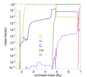
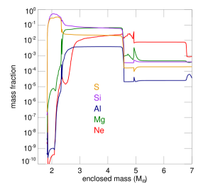
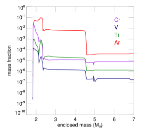
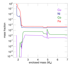
Figure 1: The curves show elemental mass fractions as a function of the enclosed mass in our supernova ejecta model computed with the mesa code for the $20\,M_{\odot}$ progenitor model of Paxton et al. (2015). Radioactive isotopes with half-lives $<10\,\text{yr}$ were replaced into their stable daughter decay products (see Appendix, Table 12).

The core collapse was simulated by excising the central $1.825\,M_{\odot}$ and placing a reflecting hydrodynamic boundary at that mass coordinate. The explosion was driven by depositing $2.3\times 10^{51}\,\textrm{ergs}$ of thermal energy over a mass coordinate range $\Delta M=0.05\,M_{\odot}$ adjacent to the excised region over the course of $1$ second. The deposition launched an outward-propagating shock wave. Explosive nucleosynthesis in the shock-heated ejecta was followed through freezeout for $60$ seconds when the kinetic energy had dropped to $1.27\times 10^{51}\,\textrm{ergs}$. The mesa calculation gives isotope-specific yields with isotopic half-lives varying over a wide range. For simplicity, we converted the isotopes with half-lives shorter than $10\,\text{yr}$ into their stable daughter isotopes. The resulting isotopes all had half-lives longer than $30\,\text{yr}$. In the dust synthesis calculation we do not distinguish between isotopes; the isotope (unstable and stable) to element conversion scheme is given in Table 12 in the Appendix. In Figure 1 we show elemental mass fraction $X_{i}$ as a function of the enclosed mass $M_{\text{ej,1987A}}$.

The model implies the following stratification of the progenitor star: the neutron star ($M<1.825\,M_{\odot}$), the explosively synthesized iron group ($1.825\,M_{\odot}<M<1.892\,M_{\odot}$), the lighter element ejecta ($1.892\,M_{\odot}<M<6.8\,M_{\odot}$), and the hydrogen envelope ($6.8\,M_{\odot}<M<14.5\,M_{\odot}$). The mass coordinate extent of ⁵⁶Ni was set found to be $M_{\rm Ni}=0.068\,M_{\odot}$, a value consistent with the range allowed by observations of SN 1987A. The boundary between the helium core and the hydrogen envelope was set where the hydrogen mass fraction dropped to a negligible value $10^{-10}$. The mass of helium and lighter element “core” ejecta was $M_{\rm core}\approx 5\,M_{\odot}$.

While the mesa calculation preserves the initial elemental stratification, we take the ⁵⁶Ni to be “dredged-up” into discrete clumps that end up randomly distributed in the core ejecta; we call these clumps “bubbles” (see Section 1). The radioactive energy released when the ⁵⁶Ni in the bubbles decayed into ⁵⁶Co (and to a lesser extent when the ⁵⁶Co decayed into ⁵⁶Fe) over-pressured the bubbles against the surrounding core ejecta and for a period of time, the nickel bubbles expanded super-homologously. The super-homologous expansion stopped when the bubbles became optically thin to the $\gamma$-rays emitted in the radioactive decays. By the start our dust-synthesis simulations, at 100 days after the explosion, the bubbles have returned to homologous expansion but occupy an elevated fraction of the volume of the helium core. We assume that the bubble expansion has swept up thin shells of the surrounding core ejecta. In Figure 2 we show a schematic diagram of the geometry of our model.

At the end of super-homologous bubble expansion, the ejecta had the following structure: low density Ni, Co, and Fe bubbles with a total mass equal to the Ni mass $M_{\rm bub}=M_{\rm Ni}$ occupying a fraction $f_{\rm Ni}$ of the volume of the helium core, multiple high density shells of swept up core ejecta with total mass:

$$M_{\rm shell}=\frac{\omega f_{\rm bub}-M_{\rm Ni}/M_{\rm core}}{\omega-M_{\rm bub}/M_{\rm core}}(M_{\rm core}-M_{\rm bub}),$$ (8)

where the density in the bubbles immediately after the explosion (before super-homologous expansion) was assumed to be $\omega$ times the mean density, and intermediate density ambient ejecta outside of the bubbles and shells with mass $M_{\rm amb}=M_{\rm core}-M_{\rm bub}-M_{\rm shell}$.

With these assumptions, the mass density in each of the three regions evolves under homologous expansion as:

$$\rho_{\rm bub,shell,amb}(t)=\rho_{\rm bub,shell,amb}(t_{0})\left(\frac{t}{t_{0}}\right)^{-3}.$$ (9)

Let $\eta$ denote the ratio of shell thickness to bubble radius. Then the density normalization factors are:

$$\rho_{\rm bub}(t_{0}) = \frac{3M_{\rm Ni}}{4\pi f_{\rm Ni}v_{\rm core}^{3}t_{0}^{3}},$$

$$\rho_{\rm amb}(t_{0}) = \frac{3({M_{\rm core}-M_{\rm Ni}})}{4\pi v_{\rm core}^{3}t_{0}^{3}}\left(1-\frac{M_{\rm Ni}}{\omega M_{\rm core}}\right)^{-1},$$

$$\rho_{\rm shell}(t_{0}) = \frac{\rho_{\rm amb}(t_{0})}{3\eta+3\eta^{2}+\eta^{3}}\left(1-\frac{M_{\rm Ni}}{\omega f_{\rm Ni}M_{\rm core}}\right),$$ (10)

where $v_{\rm core}$ is the expansion velocity at the edge of the helium core.

For the above parameters we take $v_{\rm core}=2100\,\textrm{km}\,\textrm{s}^{-1}$ (Fu & Arnett, 1989), $f_{\rm Ni}=0.5$ (Li et al., 1993), $\omega=3$ (Basko, 1994), $M_{\rm core}=5\,M_{\odot}$, and $M_{\rm Ni}=0.068\,M_{\odot}$. While the physically correct value of shell thickness could be $\eta\sim 0.01$ (Basko, 1994; Wang, 2005), because the simulation of such thin, and therefore dense, shells is computationally expensive, for practical reasons we assume thicker shells $\eta\approx 0.1$ in our fiducial simulation, and separately explore the scaling of the results in the limit of thin shells. Using these parameters gives $M_{\rm shell}=2.45\,M_{\odot}$ and $M_{\rm amb}=2.48\,M_{\odot}$. Thus outside of the nickel bubbles a fraction $f_{\rm shell}=0.498$ of the mass is in shells and $f_{\rm amb}=0.502$ is in the ambient ejecta. Evaluating Equation (2.4) we obtain, for the bubble and ambient densities, $\rho_{\rm bub}(t_{0})=1.1\times 10^{-14}\,\text{g}\,\text{cm}^{-3}$ and $\rho_{\rm amb}(t_{0})=3.9\times 10^{-13}\,\text{g}\,\text{cm}^{-3}$. The shell densities depend on the shell thickness parameter. For the shell densities we obtain $\rho_{{\rm shell},\eta=0.1}(t_{0})=1.2\times 10^{-12}\,\text{g}\,\text{cm}^{-3}$ and $\rho_{{\rm shell},\eta=0.01}(t_{0})=1.3\times 10^{-11}\,\text{g}\,\text{cm}^{-3}$.

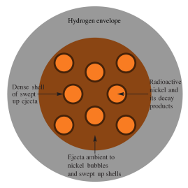
Figure 2: The figure provides a schematic illustration, not to scale, of how we model the density structure of the ejecta. We define three regions, each of uniform density, corresponding to the low density interiors of nickel bubbles, the high density shells of the material swept up by the expanding bubbles, and an intermediate density region unaffected by the bubbles.

We perform dust synthesis calculations on a grid of ejecta mass coordinates. For the bubble ejecta within $1.825\,M_{\odot}\leq M<1.892\,M_{\odot}$ we lay a grid with spacing $\Delta M=0.01\,M_{\odot}$ and run our calculations separately at each coordinate. The elemental composition in each run is taken from the mesa calculation whereas the density and temperature are chosen as appropriate for bubble interiors. The density is as given in Equations (9) and (2.4) and the temperature we discuss in the following section. The results of these runs are used to determine the properties of dust formed in the bubbles. For the shell and ambient ejecta within $1.892\,M_{\odot}\leq M<6.8\,M_{\odot}$ we choose a set of mass coordinates separated by $\Delta M=0.1\,M_{\odot}$ and run our code twice at each coordinate. The two runs at the same mass coordinate have the same composition but different densities and temperatures. One run has a temperature and density appropriate for the shells and the other for the ambient ejecta.

2.5 Thermal evolution

The ejecta thermal evolution is governed by the radioactive energy input. After ⁵⁶Ni and ⁵⁷Ni have decayed, the heating is due, in increasing order of the half-life, to ⁵⁶Co, ⁵⁷Co, ²²Na, and finally ⁴⁴Ti. We used the radiation transfer code cloudy (Ferland et al., 2013) to create a model for the gas temperature evolution. The cloudy calculation is not designed to accurately capture the geometry of radiative energy input and transfer within the ejecta. Therefore, it cannot be used to predict the normalization of the temperature, but only its variation in time. We normalize the temperature evolution by recalibrating a cloudy integration to astronomical measurements of the temperature. This approach allows us to extrapolate the temperature evolution past the first $1000\,\text{d}$ when measurements of the temperature are not available. We believe that the temperature evolution obtained through this heuristic procedure is more realistic than the power-law models invoked in published computations of dust synthesis in supernovae. In fact, we find that the ejecta temperature does not decrease in a power-law fashion.

Source	$E$ (keV)	$L$ (erg s-1)
$e^{\pm}$, X-ray	1	$3.39\times 10^{40}\times e^{-t/111.3\>\rm d}$
		$+\,9.4\times 10^{37}\times e^{-t/391.2\>\rm d}$
		$+\,1.45\times 10^{34}\times e^{-t/78\>\rm yr}$
		$+\,2.39\times 10^{36}\times e^{-t/3.75\>\rm yr}$
56Co $\gamma$-ray	1243	$9.73\times 10^{41}\times e^{-t/111.3\>\rm d}$
57Co $\gamma$-ray	115.2	$5.06\times 10^{38}\times e^{-t/391.2\>\rm d}$
44Ti $\gamma$-ray	73.24	$5.14\times 10^{35}\times e^{-t/78\>\rm yr}$
44Sc $\gamma$-ray	738.3	$7.91\times 10^{36}\times e^{-t/78\>\rm yr}$
22Na $\gamma$-ray	782.9	$1.64\times 10^{35}\times e^{-t/3.75\>\rm yr}$

Table 4: Radioactive emission energies and total luminosities used in the cloudy calculations.

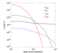
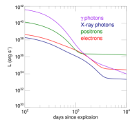
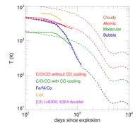
Figure 3: The curves show the rate at which energy is deposited in the ejecta by the radioactive decay of four isotopes (left panel) and via four radioactive emission channels (middle panel), and temperature evolution in SN 1987A (right panel). For a comparison of the energy deposition rates and compiled optical and far IR light curves of SN 1987A please see Figure 2 of McCray & Fransson (2016). The energy deposition channels in the middle panel are classified by the initial energy injecting particle and account for all of the secondary processes excited by the injection event. The right panel shows: observationally inferred temperatures in SN 1987A (solid lines) and our rescaled cloudy temperature evolutions (dashed lines). The orange (assuming atomic C and O) and purple (assuming molecular CO) solid lines are from Liu & Dalgarno (1995), the blue from Li et al. (1993), the green from Li & McCray (1993), and the red from Li & McCray (1992). Please see text for detail.

Specifically, we first use cloudy to compute the temperature of an optically-thin singe zone at distance $R(t)=2.16\times 10^{15}\,\textrm{cm}(t/100\,\textrm{days})$ from a point source and receding from the source with radial velocity $v=2,500\,\text{km}\,\text{s}^{-1}$. The zone has atomic number density $8.8\times 10^{9}\,\textrm{cm}^{-3}(t/100\,\textrm{days})^{-3}$ and fiducial adopted atomic concentrations in the proportion $\text{C}:\text{O}:\text{Mg}:\text{Al}:\text{Si}:\text{S}:\text{Fe}=0.25:0.25:0.1:0.1:0.1:0.1:0.1$. The single zone is irradiated by a source with a luminosity equal to the rate at which energy is released during radioactive decay (excepting the portion of the radioactive energy released in neutrinos). We take the source to emit photons at 6 discrete energies, 5 of which are produced directly in the decays and the 6th is an artificial source of 1 keV photons crudely representing the energy deposited as X-rays, electrons, and positrons. The photon energies and luminosities as a function of time for each discrete energy are given in Table 4 and are plotted in Figure 3. During the first 900 days our computed luminosity agrees with the empirical bolometric luminosity of SN 1987A (Suntzeff & Bouchet, 1990; Bouchet et al., 1991).

We ran the cloudy calculation on a temporal grid with 100 day spacing that spans the post-explosion period from $100$ to $10^{4}$ days. This provides an instantaneous temperature model $T_{\textsc{cloudy}}(t)$ at every epoch. The raw thermal evolution generated this way cannot be taken at face value because it ignores radiation transfer effects, spatial variation in chemical composition, and spatial variation in density. We recalibrate by uniform rescaling the cloudy model to empirical estimates of the temperature in SN 1987A. The recalibration is empirical and heuristic; it is justified by the close match between the recalibrated and measured temperature during the first $\sim 1000$ days. In particular, the recalibration can be construed as accounting for all the optical depth effects and the incompleteness of the inventory of molecular coolants included in cloudy. The atomic temperature track is in reasonable agreement with the calculations shown in Figures 7 and 10 of Fransson & Chevalier (1989) that cover the thermal evolution from 200 to 950 days.

In the right panel of Figure 3 we show key measurements of the ejecta temperature. Liu & Dalgarno (1995) estimated the temperature assuming that heating is from radioactive decay of ⁵⁶Co, whereas cooling is from adiabatic expansion, free-free emission, recombination, C and O lines, and vibrational CO lines. In their model, the ejecta consists of equal parts of C and O. In this mixture, CO is destroyed by Compton electrons from radioactive decay and created by radiative association of C and O (they provide a separate estimate, also shown in the figure, with CO formation disabled). Li et al. (1993) estimated the temperature in the nickel-rich regions by taking into account radioactive heating and Fe, Co, and Ni line emission cooling. Li & McCray (1993) analyzed Ca II emission lines in the hydrogen envelope ejecta. Li & McCray (1992) analyzed the flux and profile of two forbidden O I emission lines. They found that to match observations the oxygen must be absent at velocities $\lesssim 300\,\text{km}\,\text{s}^{-1}$ whereas $0.66\,M_{\odot}$ of oxygen occupies $10\%$ of the volume at velocities $300\,\text{km}\,\text{s}^{-1}<v<1400\,\text{km}\,\text{s}^{-1}$ and $0.64\,M_{\odot}$ occupies $5\%$ of the volume at $1400\,\text{km}\,\text{s}^{-1}<v<2100\,\text{km}\,\text{s}^{-1}$. The fact that the temperatures estimated from the forbidden O I lines overlap with those derived from Liu & Dalgarno (1995) with CO cooling disabled suggests that much of the oxygen may be where molecules are not able to form and cool the gas.

We use the estimates of Liu & Dalgarno (1995) to normalize our time evolution of temperature in the shells and the ambient gas. For dense shells, where molecules should be able to form, we use the estimates with CO formation enabled. In Figure 3, right panel, we show the unnormalized $T_{\textsc{cloudy}}$ and the normalized shell temperature $T_{\rm shell}(t)=0.16\,T_{\textsc{cloudy}}(t)$. For the ambient ejecta, to match the atomic gas temperature estimate, we normalize as $T_{\rm amb}(t)=0.39\,T_{\textsc{cloudy}}(t)$. We use the observed Fe-Co-Ni temperatures from Li et al. (1993) to construct a hybrid temperature model for the bubbles. In the interval $200\,\textrm{d}<t<1200\,\textrm{d}$, where temperature data are available, we use a parametric fit to the observations. Outside of this period, we continuously extrapolate with an appropriately normalized cloudy temperature evolution:

$$T_{\rm bub}(t)=\left\{\begin{array}[]{ll}\epsilon_{1}\,T_{\textsc{cloudy}}(t),&t<200\,\textrm{d},\\ 10^{\epsilon_{2}+\epsilon_{3}x+\epsilon_{4}x^{2}}\,\textrm{K},&200\,\textrm{d}<t<1200\,\textrm{d},\\ \epsilon_{5}\,T_{\textsc{cloudy}}(t),&t>1200\,\textrm{d},\end{array}\right.$$ (11)

where $x=\log_{10}(t/\,\textrm{day})$ and the coefficients are: $\epsilon_{1}=0.411$, $\epsilon_{2}=-10.5$, $\epsilon_{3}=12.1$, $\epsilon_{4}=-2.57$, and $\epsilon_{5}=0.369$. For the sake of reproducibility, here we provide a fitting function for $T_{\textsc{cloudy}}$, valid for post-explosion times $100\,\textrm{d}<t<10,000\,\textrm{d}$: $T_{\textsc{cloudy}}(t)=\sum_{i=1}^{6}\xi_{i}e^{-t/t_{i}}$ where $t_{i}=100\,\text{d}+500\,(i-1)\,\text{d}$, $\xi_{1}=7012\,\textrm{K}$, $\xi_{2}=-4588\,\textrm{K}$, $\xi_{3}=-27530\,\textrm{K}$, $\xi_{4}=155300\,\textrm{K}$, $\xi_{5}=-195200\,\textrm{K}$, and $\xi_{6}=81770\,\textrm{K}$.

We assume that this temperature model applies throughout each of the three zones. This is a very crude and ultimately incorrect assumption, though one without which our first attempt at a comprehensive dust synthesis calculation would have proven unmanageable. In reality, the energy emitted in the form of $e^{\pm}$ and X-rays is deposited essentially locally as the mean free path of an electron or an X-ray is much smaller, by a factor of at least $10^{5}$ (for $e^{\pm}$) and at least $10^{2}$ (for X-rays), than the radius of the ejecta. The mean free path for $\gamma$-ray absorption is much longer in comparison, e.g., for 1 MeV $\gamma$-rays it starts shorter than the radius of the ejecta but eventually becomes almost $10^{3}$ times longer. The ejecta become optically thin to $\gamma$-rays at $\sim 360$–$560\,\text{days}$ depending on the photon energy. Ideally, the radiation transfer effects should be modeled realistically.

In the course of revising this manuscript in response to the referee’s comments we performed a test of the thermal evolution model presented in this section. In the test we carried out a more accurate but simplified direct computation of the gas temperature. We assumed that the ejecta consisted entirely of O and CO. To compute the O cooling rate we take electron collision strengths for the lowest 5 energy levels of neutral oxygen from Draine (2011). For the CO cooling rate we used the tabulated rotational and vibrational CO cooling rates from Neufeld & Kaufman (1993) with corrections from Glover et al. (2010). In this simplified calculation we assumed that the molecular and ionization fractions were both 1% and the density equaled the average density of the ejecta. We obtained the temperature by equating the cooling rate to the radioactive heating rate using the Sobolev approximation for the optical depth. We found that compared to the simplified calculation not relying on cloudy, the cloudy-based model overestimates the temperature between 1000 and 3000 days and underestimates the temperature thereafter. The simplified model also exhibits a more substantial late increase of temperature which brings into focus the complicated interplay of cooling and radioactive heating.

3 Chemistry

Immediately after a supernova explosion, the ejecta is ionized gas. As the ejecta expand and cool, the ions recombine into atoms and molecules form via gas-phase chemical reactions. Some molecules grow large enough to become what might be called condensation nuclei, which can grow into small grains via accretion. These grains can then grow into larger grains by accretion and coagulation or diminish by evaporation and chemical weathering. To model the initial steps of the gas-to-dust transformation in supernova ejecta, the abundances of molecular species must be explicitly followed. The processes that modify molecular abundances, such as gas-phase chemical reactions, reactions with and accretion onto grains, and destruction by Compton electrons, are incorporated into the abundance evolution calculations. We proceed to describe how this is done in our simulation.

3.1 Reaction network

Category	Species
Atoms	He, C, O, Ne, Mg, Al, Si, S, Ar, Fe
Molecules	CO, C2, O2, SO, SiO, SiC, Fe2, FeO,
	Mg2, MgO, Si2, AlO, FeS, MgS
	C3, SiO2, Fe3, Mg3, Si3
	C4, Fe4, Mg4, Si4, Si2O2, Al2O2,
	Fe2O2, Fe2S2, Mg2O2, Mg2S2, Si2C2
	Si2O3, Al2O3, Fe2O3
	MgSi2O3, Si3O3, Fe3O3, Fe3S3,
	Mg3O3, Mg3S3, Si2O4
	MgSi2O4, Si3O4, Fe3O4
	Mg2Si2O4, Si4O4, Fe4O4, Fe4S4,
	Mg4O4, Mg4S4
	Mg2Si2O5, Si4O5
	Mg3Si2O5, Mg2Si2O6, Si5O5, Al4O6
	Mg3Si2O6
	Mg3Si2O7
	Mg4Si2O7
	Mg4Si2O8, Fe6O8
Ions	$e^{-}$
	He+, C+, O+, Ne+, Mg+, Al+, Si+, S+, Ar+, Fe+
	CO+, C${}_{2}^{+}$, O${}_{2}^{+}$, SO+, SiO+, SiC+, Fe${}_{2}^{+}$, FeO+,
	Mg${}_{2}^{+}$, MgO+, Si${}_{2}^{+}$, AlO+, FeS+, MgS+

Table 5: Atomic, molecular, and ionic species included in the simulation classified by the number of atoms per molecule.

Let $\mathcal{N}_{\rm S}$ be the total number of chemical species that we do not treat as dust grains (grains will be added to the picture in Section 4). The chemical species include atoms, molecules, ions, free electrons, and atomic and molecular clusters, the latter being grain condensation nuclei. The species are listed in Table 5. We explicitly follow the number density $c_{i}(t)$ of species $i$, where $i=1,\,...,\,\mathcal{N}_{\rm S}$, as a function of post-explosion time $t$. The number density of each species changes due to gas-phase chemical reactions, chemical reactions with, or catalyzed by dust grains, accretion onto and evaporation from grains, collisions with Compton electrons, and expansion of the ejecta. The number densities $c_{i}(t)$ obey a system of coupled ordinary differential equations.

We include a total of $\mathcal{N}_{\rm R}=341$ gas-phase chemical reactions. We allow up to 3 reactants and up to 3 products in each reaction. Reaction $j$, where $j=1,\,...,\,\mathcal{N}_{\rm R}$, can be written in the form:

$$R_{1}(j)+R_{2}(j)+R_{3}(j)\to P_{1}(j)+P_{2}(j)+P_{3}(j),$$ (12)

where $R_{k}(j)$ is the $k$th reactant in reaction $j$ and $P_{k}(j)$ is the $k$th product in reaction $j$. If there are fewer than three reactants or products, we set the extra ones to zero.

Each reaction $j$ has a gas-temperature-dependent rate coefficient $k_{j}(T)$. The rate coefficients are written in the Arrhenius form:

$$k_{j}(T)=A_{j}\left(\frac{T}{300\,\textrm{K}}\right)^{\nu_{j}}e^{-E_{\rm a,\it j}/{k_{\rm B}}T},$$ (13)

where $A_{j}$, $\nu_{j}$, and $E_{\rm a,\it j}$ are reaction-specific constants. The exponent $\nu_{j}$ is dimensionless. The activation energy $E_{\rm a,\it j}$ has the units of energy but is usually expressed as a temperature $T_{\rm A,\it j}=E_{\rm a,\it j}/{k_{\rm B}}$. The units of the coefficient $A_{j}$ depend on the number of reactants: s^-1 for one reactant, cm³ s^-1 for two, and cm⁶ s^-1 for three. Reaction $j$ has a rate per unit volume $k_{j}(T)c_{R_{1}(j)}c_{R_{2}(j)}c_{R_{3}(j)}$, where $c_{R_{3}(j)}=1$ if there are two reactants and $c_{R_{2}(j)}=c_{R_{3}(j)}=1$ if there is only one reactant.

The time derivative of the number density of species $i$ due to gas-phase chemical reactions is:

$$\left(\frac{dc_{i}}{dt}\right)_{\text{chem}}=\sum_{j=1}^{\mathcal{N}_{\rm R}}(\alpha_{ij}-\beta_{ij})k_{j}(T)c_{R_{1}(j)}c_{R_{2}(j)}c_{R_{3}(j)}$$ (14)

where $\alpha_{ij}$ and $\beta_{ij}$ are the number of times that species $i$ occurs as, respectively, a product and a reactant in reaction $j$.

3.2 The rate coefficients

The chemical reactions that we include in our simulations are given in Tables 13 through 39 (hereafter referred to as the “reaction tables"). The tables give, for each reaction $j$, the Arrhenius rate coefficient parameters $A_{j}$, $\nu_{j}$, and $T_{0,j}$. The numerical values of these parameters were taken from the literature when possible. Unfortunately, not all reactions relevant to dust formation have measured or calculated rates, and the rates of those that do are only valid in certain temperature and pressure range. In some cases, as we outline here, we have had to perform informed extrapolations of the measured or calculated rates.

The coefficient for a two-body reaction $\mbox{A}+\mbox{B}\to\mbox{C}+\mbox{D}$ is given by a thermal average of the reaction cross section multiplied by the relative velocity $v_{\text{AB}}$

$$k_{\rm AB}=\pi(r_{\rm A}+r_{\rm B})^{2}\sqrt{\frac{8{k_{\rm B}}T}{\pi\mu_{\rm AB}}}\left(1+\frac{E_{\rm a,AB}}{{k_{\rm B}}T}\right)e^{-E_{\rm a,AB}/{k_{\rm B}}T},$$ (15)

where $r_{i}$ is the molecular radius of species $i$, $\mu_{AB}$ is the reduced mass, and $E_{\rm a,AB}$ is the activation energy (which may be zero). This expression for the rate coefficient is not in Arrhenius form. If the activation energy is zero or much less than ${k_{\rm B}}T$, then all terms involving $E_{\rm a,AB}$ vanish and the rate coefficient is in Arrhenius form. On the other hand, if $E_{\rm a,AB}\gg{k_{\rm B}}T$ then $1+E_{\rm a,AB}/{k_{\rm B}}T$ can be replaced with $E_{\rm a,AB}/{k_{\rm B}}T$ and again the rate coefficient is in Arrhenius form.

A three-body reaction of the form $\mbox{A}+\mbox{B}+\mbox{M}\to\mbox{AB}+\mbox{M}$, where M is any gas particle, takes place in two steps. First an A particle collides with a B particle forming an unstable transition state AB^∗. Then a gas particle M collides with the transition state and removes enough of the energy of the transition state to leave it in the form of a stable AB molecule. The rate coefficient $k^{*}_{\rm AB}$ for the formation of the transition state is obtained by setting the activation energy to zero in Equation (15).

Once the transition state forms, it has a lifetime $\tau^{*}_{\rm AB}$ during which it can fragment back into A and B. The mean time between collisions with a third body for a given transition state molecule is:

$$\tau_{\rm col,AB}=\frac{1}{c_{\rm tot}(\left\langle r\right\rangle+r_{\rm AB})^{2}}\left(\frac{8\pi{k_{\rm B}}T}{\left\langle m\right\rangle}+\frac{8\pi{k_{\rm B}}T}{m_{\rm AB}}\right)^{-1/2},$$ (16)

where $c_{\rm tot}$ is the total number density of all gas species, $\left\langle r\right\rangle$ is the average radius of a gas particle, $\left\langle m\right\rangle$ is the mean molecular weight, $r_{\rm AB}$ is the radius of the transition state, and $m_{\rm AB}=m_{\rm A}+m_{\rm B}$ is the mass of the transition state.

If $\tau_{\rm col,AB}>\tau_{\rm AB}^{*}$, the number density of transition state molecules is $c_{\rm AB}^{*}=c_{\rm A}c_{\rm B}k_{\rm AB}^{*}\tau_{\rm AB}^{*}$ and so the rate per unit volume of the overall three-body reaction is $c_{\rm AB}^{*}c_{\rm tot}k^{\prime}=c_{\rm A}c_{\rm B}k_{\rm AB}^{*}\tau_{\rm AB}^{*}c_{\rm tot}k_{\rm AB}^{\prime}$, where:

$$k_{\rm AB}^{\prime}=(r_{\rm AB}+\left\langle r\right\rangle)^{2}\left(\frac{8\pi{k_{\rm B}}T}{\left\langle m\right\rangle}+\frac{8\pi{k_{\rm B}}T}{m_{\rm AB}}\right)^{1/2}.$$ (17)

Thus the overall volumetric three-body reaction rate can be written as $k_{3,{\rm AB}}c_{\rm A}c_{\rm B}c_{\rm tot}$ with $k_{3,{\rm AB}}=k_{\rm AB}^{*}\tau_{\rm AB}^{*}k_{\rm AB}^{\prime}$. If, on the other hand, $\tau_{\rm col,AB}<\tau_{\rm AB}^{*}$, then we can assume that a third body M will collide with the transition state before it fragments and thus we can replace the reaction $\mbox{A}+\mbox{B}+\mbox{M}\to\mbox{AB}+\mbox{M}$ with $\mbox{A}+\mbox{B}\to\mbox{AB}$. The rate coefficient for this reaction is again as given in Equation (15).

For simplicity we assume that $\tau_{\rm AB}^{*}=2\pi/\omega_{0}=1.52\times 10^{-13}\,\textrm{s}$, where $\omega_{0}=4.12\times 10^{13}\,\textrm{s}^{-1}$ is the angular frequency of bonds in an Einstein solid made of carbon. Effectively we are approximating the lifetime of the transition state as the vibrational period of the bond holding the transition state molecule together. We are also assuming that this vibrational period is similar to that of a carbon Einstein solid. Then, with $r_{\rm A}=r_{\rm B}=6.7\times 10^{-9}\,\textrm{cm}$ (the radius of a carbon atom), $m_{\rm A}=m_{\rm B}=12.0\,\textrm{amu}$ (the mass of a carbon atom), $\left\langle m\right\rangle=12.0\,\textrm{amu}$, and $\left\langle r\right\rangle=4.69\times 10^{-9}\,\textrm{cm}$ gives a three-body reaction coefficient with Arrhenius parameters $A=4.253\times 10^{-34}\,\textrm{cm}^{6}\,\textrm{s}^{-1}$, $\nu=+1$, and $T_{0}=0$ (where the latter indicates that we are assuming there is no activation energy). We use these parameters for all three-body reactions; they agree with experimental values in the common temperature range of validity but give rates that behave well at low temperatures.

The reactions involving the formation of enstatite and forsterite dimers were taken from Goumans & Bromley (2012). The reference describes how gas phase reactions can build up silicates such as enstatite and forsterite dimers starting with SiO as the seed. Each reaction in their paper involves either addition of a Si or Mg atom or oxidation by H₂O. Since in our model, hydrogen is absent in the dust-forming-ejecta of SN 1987A, we follow the approach of Sarangi & Cherchneff (2013) and substitute O₂ and SO for the H₂O in Goumans & Bromley (2012). Tables providing all the reactions rates are available in electronic form at MNRAS online.

3.3 Destruction by Compton electrons

In Section 2 we discussed how radioactivity produces a population of high energy electrons (and positrons), the so-called Compton electrons, that can go on to ionize atoms and molecules and dissociate molecules. We include the following “destruction by Compton electron" reactions. For each neutral atomic species X we include a reaction of the form:

$$\mbox{X}+e^{-}_{*}\to\mbox{X}^{+}+e^{-}+e^{-}_{*},$$ (18)

where $e^{-}_{*}$ denotes the Compton electron. For each neutral diatomic molecule AB we include the following four reactions:

$$\mbox{AB}+e^{-}_{*} \to \mbox{AB}^{+}+e^{-}+e^{-}_{*},$$

$$\mbox{AB}+e^{-}_{*} \to \mbox{A}+\mbox{B}+e^{-}_{*},$$

$$\mbox{AB}+e^{-}_{*} \to \mbox{A}^{+}+\mbox{B}+e^{-}+e^{-}_{*},$$

$$\mbox{AB}+e^{-}_{*} \to \mbox{A}+\mbox{B}^{+}+e^{-}+e^{-}_{*}.$$ (19)

For triatomic and larger molecules we ignore reactions with Compton electrons.

Type	Reaction	$W_{i}^{j}$ (eV)
Ionization (Atoms)	$\mbox{X}\to\mbox{X}^{+}+e^{-}$	47
Ionization (Molecules)	$\mbox{AB}\to\mbox{AB}^{+}+e^{-}$	34
Dissociation	$\mbox{AB}\to\mbox{A}+\mbox{B}$	125
Dissociative Ionization	$\mbox{O}_{2}\to\mbox{O}^{+}+\mbox{O}+e^{-}$	768
	$\mbox{AO}\to\mbox{A}^{+}+\mbox{O}+e^{-}$	247
	$\mbox{AO}\to\mbox{A}+\mbox{O}^{+}+e^{-}$	768
	$\mbox{AB}\to\mbox{A}^{+}+\mbox{B}+e^{-}$	247

Table 6: Energy lost by Compton electrons per reaction. In dissociative ionization, $\text{A},\text{B}\neq\text{O}$. The values of $W_{i}^{j}$ are from Cherchneff & Dwek (2009).

To find the rate coefficient for reactions with Compton electrons we model the total energy per unit time that goes into ionization and dissociation by multiplying $L(t)$ in Equation (3) with a dimensionless factor $L_{\rm ion}(t)=f_{\rm ion}\,L(t)$. We assume that this energy is equally distributed among all gas particles. If $N_{\rm tot}$ is the total number of particles in the ejecta, then the rate at which ionizing energy is deposited directly onto an atom or molecule is $L_{\rm ion}/N_{\rm tot}$. For each species $i$ there are $\mathcal{N}_{i}^{\rm C}$ possible reactions that can be induced by Compton electrons (ionization, dissociation, etc.). In each reaction $j$ the Compton electron loses an energy $W_{i}^{j}$ so the rate coefficient for reaction $j$ is

$$k_{i,j}^{\rm C}=\frac{L_{\rm ion}}{N_{\rm tot}\,W_{i}^{j}}.$$ (20)

The rate per unit volume of reaction $j$ is $k_{i,j}^{\rm C}c_{i}$. See Table 6 for the values of $W_{i}^{j}$.

For convenience we give the time derivatives of the number densities of the species affected by Compton electron destruction reactions. For each neutral atomic species X we have

$$\left(\frac{dc_{\rm X}}{dt}\right)_{\rm Compt}=-\left(\frac{dc_{{\rm X^{+}},e^{-}}}{dt}\right)_{\rm Compt}=-k_{0}c_{\rm X},$$ (21)

where $k_{0}=L_{\rm ion}/(N_{\rm tot}\times 47.0\,\textrm{eV})$. For each neutral diatomic molecular species AB we have:

$$\left(\frac{dc_{\rm AB}}{dt}\right)_{\rm Compt} = -(k_{1}+k_{2}+k_{3}+k_{4})c_{\rm AB},$$

$$\left(\frac{dc_{\rm AB^{+}}}{dt}\right)_{\rm Compt} = k_{1}c_{\rm AB},$$

$$\left(\frac{dc_{\rm A^{+}}}{dt}\right)_{\rm Compt} = k_{3}c_{\rm AB},$$

$$\left(\frac{dc_{\rm B^{+}}}{dt}\right)_{\rm Compt} = k_{4}c_{\rm AB},$$

$$\left(\frac{dc_{\rm A}}{dt}\right)_{\rm Compt} = (k_{2}+k_{4})c_{\rm AB},$$

$$\left(\frac{dc_{\rm B}}{dt}\right)_{\rm Compt} = (k_{2}+k_{3})c_{\rm AB},$$

$$\left(\frac{dc_{e^{-}}}{dt}\right)_{\rm Compt} = (k_{1}+k_{3}+k_{4})c_{\rm AB},$$ (22)

where $k_{i}=L_{\rm ion}/N_{\rm tot}W_{i}$. Here, $W_{1...4}=(34,\,125,\,247,\,247)\,\text{eV}$ in reactions not producing ionized oxygen, and the same except for the replacement $247\,\text{eV}\rightarrow 768\,\text{eV}$ in reactions producing O⁺.

3.4 The nucleation of C clusters

As an example we mention the main chemical reactions participating in the formation of carbon clusters. The main route to forming carbon grain condensation nuclei, which we take to be the clusters with 4 carbon atoms (C₄), involves the following monomer inclusion reactions $\text{C}+\text{C}_{n}\rightarrow\text{C}_{n+1}+\gamma$ for $n=(1,2,3)$ as well as $\text{C}_{2}+\text{C}_{2}\rightarrow\text{C}_{4}+\gamma$. Oxygen atoms disrupt this chain at several points. First, $\text{C}+\text{O}\rightarrow\text{CO}+\gamma$ sequesters some carbon atoms so that they cannot be incorporated in clusters. This is somewhat offset by the Compton electron induced dissociation of carbon monoxide $\text{CO}+e_{*}^{-}\rightarrow\text{C}+\text{O}+e_{*}^{-}$. Oxygen atoms also destroy carbon clusters via $\text{C}_{n}+\text{O}\rightarrow\text{C}_{n-1}+\text{CO}$. Carbon clusters can also be destroyed by reactions with noble gas ions and Compton electrons

$$\text{C}_{n}+\text{He}^{+}\rightarrow\text{C}_{n-1}+\text{He}+\text{C},\ \ \ (n=2,3,4),$$

$$\text{C}_{n}+e_{*}^{-}\rightarrow\text{C}_{n-1}+\text{C}+e_{*}^{-},\ \ \ (n=2).$$ (23)

Once C₄ forms dust grains are produced by $\text{C}_{4}+\text{C}_{n}\rightarrow\text{dust grains}$, where $n=(1,2,3,4)$.

At this point a caveat is in order. Carbon clusters, including those with $n\gg 4$, inhabit a complex configuration space where they form chains, rings, and fullerenes. The cluster geometry has a strong effect on the cluster stability as can be seen in the detailed calculations of, e.g., Mauney et al. (2015). The calculations presented in the present work could be improved (at the cost of substantial additional numerical development) by resolving all the $n\lesssim 100$ clusters by their atomic number and distinct geometric configuration with configuration-specific cohesion energies. In particular some specific chains are less stable and dust nucleation then proceeds via other pathways.

4 Grains

A dust grain is a collection of atoms and molecules that behaves as a solid body. We classify grains based on the molecular formula of the fundamental molecular constituent of the grain. When the molecular formula equals the fundamental molecular formula of a grain species, we call the molecule a monomer of the species. An object consisting of $n$ monomers of some grain species is an $n$-mer of the species. A dust grain is just an $n$-mer with a sufficiently large number of monomers.

4.1 Classification

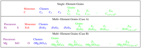
Figure 4: The diagram shows the division of dust grains into categories based on their chemical synthesis pathway. The single element grains nucleate directly from the atomic phase. The Case A multi-element grains nucleate from monomers existing in the gas phase, whereas the Case B grains nucleate from dimers that have formed in the gas phase.

Grains of pure carbon, silicon, magnesium, and iron contain only one element and are referred to as single-element grains. Let $\mathcal{X}$ denote a monomer of a single-element grain (which is just a single atom such as C, Si, Mg, or Fe) and $\mathcal{X}_{n}$ denote an $n$-mer. In our simulation we treat $\mathcal{X}$, $\mathcal{X}_{2}$, $\mathcal{X}_{3}$, and $\mathcal{X}_{4}$ as molecular species in our non-equilibrium chemistry network. Clusters with $n>4$ are treated as grains. We track the grain size distribution on a discrete grid of grain radii. The single-element grain synthesis chain consists of monomers, clusters, and grains as illustrated in Figure 4.

The monomers of multi-element grains are composed of more than one element. They can be as simple as iron sulfide (FeS) or as complex as forsterite (Mg₂SiO₄). It is convenient to divide multi-element grains into two sub-classes, Cases A and B, based on whether their monomer exists in the gas phase. Case A multi-element grains are those that have a monomer that can form in the gas phase. Here, such grains include: FeS, FeO, SiC, Al₂O₃, SiO₂, MgO, Fe₃O₄, and MgS. The first step in the formation of a Case A multi-element grain is the formation of a monomer $\mathcal{X}$ from chemical reactions involving gas-phase precursors. Later $n$-mers $\mathcal{X}_{n}$ are built from the monomers by accretion and coagulation and can eventually grow into grains. The Case A multi-element grain synthesis chain consists of precursors, monomers, clusters, and grains, as shown in the middle section of Figure 4.

Case B multi-element grains consist of monomers that cannot exist in the gas phase. We consider only two such species, enstatite (MgSiO₃) and forsterite (Mg₂SiO₄). The first step in the synthesis of Case B multi-element grains is direct gas-phase formation of a dimer $\mathcal{X}_{2}$. The dimer serves as the nucleus for $n$-merization by accretion and coagulation. The Case B multi-element grain synthesis chain also consists of precursors, clusters, and grains, as shown in the lower section of Figure 4.

The grains formed in supernovae can be heterogeneous mixtures aggregating different species, e.g., mixtures of carbon and enstatite. To curtail computational complexity, we did not consider heterogeneous grains. The effect of heterogeneity would be to deplete refractory elements from the gas phase more efficiently than predicted here.

4.2 Grain size discretization

We model dust grains as balls of densely packed monomers in the solid phase. The treatment of molecular clusters as spherical and densely packed is of course highly artificial—the clusters can in fact have linear and other aspherical geometries—but it is a necessary oversimplification that makes our comprehensive calculation tractable. Let $m_{1}$, $a_{1}$, $x_{1}=\frac{4}{3}\pi a_{1}^{3}$, and $\varrho=m_{1}/x_{1}$ denote the grain-species-specific mass, radius, volume, and density of one monomer in the solid phase. With these, $m_{n}=nm_{1}$, $a_{n}=n^{1/3}a_{1}$, $x_{n}=nx_{1}$, and $\varrho$ are the mass, radius, volume, and density of an $n$-mer.

For each grain species we track the number density of precursor $n$-mers, which we call ‘clusters’, for all consecutive $n$ up to some maximum value $n_{\rm max}$. Larger $n$-mers with $n>n_{\rm max}$ we refer to as ‘grains’. Since we cannot separately track the number densities of grains for all consecutive, large $n$, for each grain species we discretize the grain density as a function of the $n$-mer number on a logarithmic grid of grain radii labeled by index $\ell$ (recall that the radius is in one-to-one relation with the $n$-mer number and the grain volume). Let $\ell_{\rm max}$ be the number of the grid points. We set the smallest radial grid point $a_{\rm min}$ to the radius of the $(n_{\rm max}+1)$mer particle for all species except for enstatite and forsterite, for which we use the radius of the $(n_{\rm max}+2)$mer. For the maximum radius and number of grid points we use $a_{\rm max}=100\,\textrm{$\mu$m}$ and $\ell_{\rm max}=50$ for all grain species. Specifically the $\ell$th grid point is at $a_{\ell}=a_{\rm min}(a_{\rm max}/a_{\rm min})^{(\ell-1)/(\ell_{\rm max}-1)}$. To distinguish between clusters and grains, a cluster with $n$ monomers is denoted with $\mathcal{X}_{n}$, has radius $a_{n}$, mass $m_{n}$, and number density $c_{n}$. A grain associated with radial grid point $\ell$ is denoted with $\mathcal{Z}_{\ell}$, has radius $a_{\ell}$, mass $m_{\ell}$, and number density $c_{\ell}$.

4.3 Coagulation

In our simulation clusters form via chemical binding via the reactions included in our chemical reaction network. The largest $n$-mer cluster $\mathcal{X}_{n_{\rm max}}$ acting as precursor of a given grain species is referred to as the condensation nucleus. The condensation nucleus can grow into a grain by accretion of gas phase precursors or by coagulation with other clusters. It is also possible that two clusters, either or both of which can be smaller than the condensation nucleus, can merge to form a grain. We classify coagulation events based on the coagulating species and the coagulation product. The events where two clusters collide and produce a cluster are handled by the chemical reaction network. The events in which two clusters collide and result in a grain, however, are not considered chemical reactions but are genuine coagulation events. The other possibilities, including cluster-grain and grain-grain coagulation events, always lead to grains.

Coagulation is the process:

$$\mathcal{X}_{n_{1}}+\mathcal{X}_{n_{2}}\to\mathcal{X}_{n_{1}+n_{2}}$$ (24)

in which grains $\mathcal{X}_{n_{1}}$ and $\mathcal{X}_{n_{2}}$ with volumes $x_{n_{1}}$ and $x_{n_{2}}$ collide and adhere to form a new grain $\mathcal{X}_{n_{1}+n_{2}}$ with volume $x_{n_{1}+n_{2}}=x_{n_{1}}+x_{n_{2}}$. The contribution of coagulations to the rate of change of the concentration $c_{n}$ of grains $\mathcal{X}_{n}$ is:

$$\left(\frac{dc_{n}}{dt}\right)_{\rm coag}=\frac{1}{2}\sum_{i=1}^{n-1}K_{i,n-i}c_{i}c_{n-i}-\sum_{i=1}^{\infty}K_{i,n}c_{i}c_{n},$$ (25)

where $K_{i,n}$ is the temperature-dependent coagulation kernel.

We coarse-grain coagulation on our grid of grain radii (or volumes) as follows. Consider the process:

$$\mathcal{Z}_{\ell_{1}}+\mathcal{Z}_{\ell_{2}}\to\mathcal{Z}_{\ell_{1}\ell_{2}}$$ (26)

in which grains $\mathcal{Z}_{\ell_{1}}$ and $\mathcal{Z}_{\ell_{2}}$ with radii $a_{\ell_{1}}$ and $a_{\ell_{2}}$ combine to form a grain $\mathcal{Z}_{\ell_{1}\ell_{2}}$ with radius $a_{\ell_{1}\ell_{2}}=(a_{\ell_{1}}^{3}+a_{\ell_{2}}^{3})^{1/3}$. Find the radial grid point interval $[a_{k},a_{k+1})$ containing $a_{\ell_{1}\ell_{2}}$ by computing the index $\ell(\ell_{1},\ell_{2})=\lfloor(\ell_{\rm max}-1)\ln(a_{\ell_{1}\ell_{2}}/a_{\rm min})/\ln(a_{\rm max}/a_{\rm min})\rfloor+1$ and then distribute the new grain density increase between the flanking grid points:

$$\mathcal{Z}_{\ell_{1}}+\mathcal{Z}_{\ell_{2}}\to\eta_{\ell_{1}\ell_{2}}\mathcal{Z}_{\ell(\ell_{1},\ell_{2})}+(1-\eta_{\ell_{1}\ell_{2}})\mathcal{Z}_{\ell(\ell_{1},\ell_{2})+1},$$ (27)

where the mass-conserving weighting is $\eta_{\ell_{1}\ell_{2}}=(a_{\ell(\ell_{1},\ell_{2})+1}^{3}-a_{\ell_{1}\ell_{2}}^{3})/(a_{\ell(\ell_{1},\ell_{2})+1}^{3}-a_{\ell(\ell_{1},\ell_{2})}^{3})$. If the result of coagulation produces a grain with radius exceeding $a_{\rm max}$, we apportion the coagulation product to the largest radius grid point in mass conserving fashion $\mathcal{Z}_{\ell_{1}}+\mathcal{Z}_{\ell_{2}}\to\hat{\eta}_{\ell_{1}\ell_{2}}\mathcal{Z}_{\ell_{\rm max}}$, where $\hat{\eta}_{\ell_{1}\ell_{2}}=(a_{\ell_{1}\ell_{2}}/a_{\rm max})^{3}$.

The collision rate per unit volume between grains at radial grid points $\ell_{1}$ and $\ell_{2}$ with number densities $c_{\ell_{1}}$ and $c_{\ell_{2}}$ is $c_{\ell_{1}}c_{\ell_{2}}K_{\ell_{1}\ell_{2}}$ where $K_{\ell_{1}\ell_{2}}$ is the coagulation kernel:

$$K_{\ell_{1}\ell_{2}}=\mathcal{W}_{\ell_{1}\ell_{2}}\mathcal{C}_{\ell_{1}\ell_{2}}(a_{\ell_{1}}+a_{\ell_{2}})^{2}\sqrt{\frac{8\pi{k_{\rm B}}T}{\mu_{\ell_{1}\ell_{2}}}}.$$ (28)

Here, $\mu_{\ell_{1}\ell_{2}}=m_{\ell_{1}}m_{\ell_{2}}/(m_{\ell_{1}}+m_{\ell_{2}})$ is the reduced mass, $\mathcal{W}_{\ell_{1}\ell_{2}}$ is the factor by which the van der Waals force enhances the adhesion cross section, and $\mathcal{C}_{\ell_{1}\ell_{2}}$ is the factor by which the Coulomb force between electrically charged grains modifies the collision cross section. The corresponding formulas for cluster-cluster and cluster-grain collisions can be found by replacing grain number densities, radii, and masses with the corresponding cluster values as appropriate.

The rate of change of the density $c_{\ell}$ of grains $\mathcal{Z}_{\ell}$ is:

$$\left(\frac{dc_{\ell}}{dt}\right)_{\rm coag} = \sum_{\ell_{1}=1}^{\ell}\sum_{\ell_{2}=1}^{\ell_{1}}F_{\ell_{1}\ell_{2};\ell}K_{\ell_{1}\ell_{2}}c_{\ell_{1}}c_{\ell_{2}}$$ (29)

$$-c_{\ell}\sum_{\ell_{1}=1}^{\ell_{\rm max}}K_{\ell_{1}\ell}c_{\ell_{1}},$$

where $F_{\ell_{1}\ell_{2};\ell}$ is the fraction of the mass of $\mathcal{Z}_{\ell_{1}}$ and $\mathcal{Z}_{\ell_{2}}$ deposited in $\mathcal{Z}_{\ell}$:

$$F_{\ell_{1}\ell_{2};\ell}=\begin{cases}\eta_{\ell_{1}\ell_{2}},&\text{if }\ell=\ell(\ell_{1},\ell_{2})<\ell_{\rm max},\\ 1-\eta_{\ell_{1}\ell_{2}},&\text{if }\ell=\ell(\ell_{1},\ell_{2})+1\leq\ell_{\rm max},\\ \hat{\eta}_{\ell_{1}\ell_{2}},&\text{if }\ell=\ell_{\rm max}\leq\ell(\ell_{1},\ell_{2}),\\ 0,&\mbox{otherwise}.\end{cases}$$ (30)

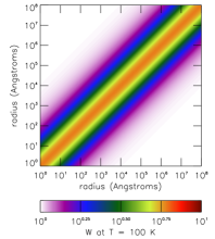
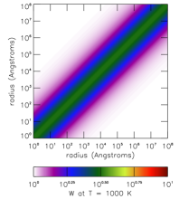
Figure 5: The contour plot shows the Van der Waals correction factor $\mathcal{W}_{\ell_{1}\ell_{2}}$ for carbon grains at four different temperatures (see Equation 31). The horizontal and vertical axes give the radii of the colliding grains. Each panel corresponds to a particular gas temperature which is given below the legend.

Species	Formula	$A$ ($10^{4}$ K) 1	$B$ 1	$\sigma_{\text{ST}}$ (erg cm-2) 1	$r_{1}$ (Å) 1	$\varrho$ (g cm-3) 2	Condensation Nucleus
Iron	Fe	4.8418	16.5566	1800	1.411	7.88069	Fe4
Silicon	Si	5.36975	17.4349	800	1.684	2.3314	Si4
Carbon	C	8.64726	19.0422	1400	1.281	2.26507	C4
Magnesium 3	Mg	7.0085	18.2386	1100	1.76917	1.74	Mg4
Forsterite	Mg2SiO4	37.24	104.872	436	2.589	3.21394	Mg4Si2O8
Iron Sulfide	FeS	9.31326	30.7771	380	1.932	4.83256	Fe4S4
Silicon Carbide	SiC	14.8934	37.3825	1800	1.702	3.22393	Si2C2
Alumina	Al2O3	18.4788	45.3543	690	1.718	7.97125	Al4O6
Enstatite	MgSiO3	25.0129	72.0015	400	2.319	7.97125	Mg2Si2O6
Silicon Dioxide	SiO2	12.6028	38.1507	605	2.08	2.64686	Si2O4
Magnesia	MgO	11.9237	33.1593	1100	1.646	3.58281	Mg4O4
Magnetite	Fe3O4	13.2889	39.1687	400	1.805	15.6078	Fe6O8
Iron Oxide	FeO	11.129	31.985	580	1.682	5.98516	Fe4O4
Magnesium Sulfide 4	MgS	9.9783	31.9071	720.69	1.89065	3.30655	Mg4S4
1 The parameters $A$, $B$, $r_{1}$, and $\sigma$ are from Nozawa et al. (2003) for all grain species except Mg and MgS.
2 The mass density was taken to be the mass of a monomer divided by $4\pi a_{1}^{3}/3$.
3 For Mg we simply averaged the parameters for C and Si.
4 The parameters for MgS were scaled from those for MgO using the FeS to FeO parameter ratios.

Table 7: Grain properties showing the species name, molecular formula, the vapor pressure coefficients $A$ and $B$, the monomer radius $r_{1}$, the surface tension $\sigma$, the mass density $\rho$, and the condensation nucleus.

Species	Smallest Grain	$a_{\rm min}$ (Å)	$A_{\rm H}$ ($10^{-12}\,\textrm{erg}$) 1,2	$T_{\text{D}}$ (K) 3,4,5	Evaporation/Accretion 6
Iron	Fe5	2.41278	30	470	$\mbox{Fe}_{n}+\mbox{Fe}\rightleftarrows\mbox{Fe}_{n+1}$
Silicon	Si5	2.8796	21	692	$\mbox{Si}_{n}+\mbox{Si}\rightleftarrows\mbox{Si}_{n+1}$
Carbon	C5	2.19048	4.7	420	$\mbox{C}_{n}+\mbox{C}\rightleftarrows\mbox{C}_{n+1}$
Magnesium	Mg5	3.02524	3.0	330	$\mbox{Mg}_{n}+\mbox{Mg}\rightleftarrows\mbox{Mg}_{n+1}$
Forsterite	Mg8Si4O16	4.10978	0.65	470	$(\mbox{Mg${}_{2}$SiO${}_{4}$})_{n}+2\mbox{Mg}+\mbox{SiO}+3\mbox{O}\rightleftarrows(\mbox{Mg${}_{2}$SiO${}_{4}$})_{n+1}$
Iron Sulfide	Fe5S5	3.30367	2.606	470	$(\mbox{FeS})_{n}+\mbox{Fe}+\mbox{S}\rightleftarrows(\mbox{FeS})_{n+1}$
Silicon Carbide	Si3C3	2.45471	4.4	470	$(\mbox{SiC})_{n}+\mbox{Si}+\mbox{C}\rightleftarrows(\mbox{SiC})_{n+1}$
Alumina	Al6O9	2.47778	1.50	470	$(\mbox{Al${}_{2}$O${}_{3}$})_{n}+2\mbox{Al}+3\mbox{O}\rightleftarrows(\mbox{Al${}_{2}$O${}_{3}$})_{n+1}$
Enstatite	Mg4Si4O12	3.68118	2.606	470	$(\mbox{MgSiO${}_{3}$})_{n}+\mbox{Mg}+\mbox{SiO}+2\mbox{O}\rightleftarrows(\mbox{MgSiO${}_{3}$})_{n+1}$
Silicon Dioxide	Si3O6	2.99988	2.606	470	$(\mbox{SiO${}_{2}$})_{n}+\mbox{SiO}+\mbox{O}\rightleftarrows(\mbox{SiO${}_{2}$})_{n+1}$
Magnesia	Mg5O5	2.81462	2.606	470	$(\mbox{MgO})_{n}+\mbox{Mg}+\mbox{O}\rightleftarrows(\mbox{MgO})_{n+1}$
Magnetite	Fe9O12	2.60326	2.606	470	$(\mbox{Fe${}_{3}$O${}_{4}$})_{n}+3\mbox{Fe}+4\mbox{O}\rightleftarrows(\mbox{Fe${}_{3}$O${}_{4}$})_{n+1}$
Iron Oxide	Fe5O5	2.87618	2.606	470	$(\mbox{FeO})_{n}+\mbox{Fe}+\mbox{O}\rightleftarrows(\mbox{FeO})_{n+1}$
Magnesium Sulfide	Mg5S5	3.23297	2.606	470	$(\mbox{MgS})_{n}+\mbox{Mg}+\mbox{S}\rightleftarrows(\mbox{MgS})_{n+1}$
1 The Hamaker constant is from Sarangi & Cherchneff (2015) for forsterite, alumina, carbon, magnesium, silicon carbide, silicon, and iron.
2 For the grain species not listed in 1, we use an average value of $A_{\rm H}=2.606\times 10^{-12}\,\textrm{erg}$.
3 For the Debye temperature we take the value for carbon and forsterite from Guhathakurta & Draine (1989).
4 The value of $T_{\text{D}}$ for magnesium and silicon is from values originally in Stewart (1983) that have since been updated various sources (not cited).
5 For the species not identified in 4 and 5 we use $T_{\text{D}}=470\,\textrm{K}$.
6 The evaporation and accretion reactions were taken from Nozawa et al. (2003).

Table 8: Additional grain properties showing the smallest grain formula and radius $a_{\text{min}}$, the Hamaker constant $A_{\rm H}$, the Debye temperature $T_{\text{D}}$, and the evaporation-accretion reaction.

4.3.1 Van der Waals correction

The van der Waals enhancement factor is (Jacobson , 2005):

$$\mathcal{W}_{\ell_{1}\ell_{2}} = -\frac{1}{2{k_{\rm B}}T(a_{\ell_{1}}+a_{\ell_{2}})^{2}}\int_{a_{\ell_{1}}+a_{\ell_{2}}}^{\infty}dr\,r^{2}\frac{d}{dr}\left(r\frac{dV_{\ell_{1}\ell_{2}}}{dr}\right)$$ (31)

$$\times e^{-(\frac{1}{2}rdV_{\ell_{1}\ell_{2}}/dr+V_{\ell_{1}\ell_{2}})/{k_{\rm B}}T},$$

where $T$ is the gas temperature, $r$ is the distance between grain centers, and $V_{\ell_{1}\ell_{2}}$ is the potential energy associated with the van der Waals force. The potential energy is:

$$V_{\ell_{1}\ell_{2}}(r) = -\frac{A_{\rm H}}{6}\left[\frac{2a_{\ell_{1}}a_{\ell_{2}}}{r^{2}-(a_{\ell_{1}}+a_{\ell_{2}})^{2}}+\frac{2a_{\ell_{1}}a_{\ell_{2}}}{r^{2}-(a_{\ell_{1}}-a_{\ell_{2}})^{2}}\right.$$ (32)

$$\left.+\ln\left(\frac{r^{2}-(a_{\ell_{1}}+a_{\ell_{2}})^{2}}{r^{2}-(a_{\ell_{1}}-a_{\ell_{2}})^{2}}\right)\right],$$

where $A_{\rm H}$ is the grain-species-specific Hamaker constant. The values of $A_{\rm H}$ can be found in Table 8. For the specific case of carbon grains, in Figure 5 we plot the van der Waals enhancement factor as a function of the colliding grain radii. The enhancement factor is maximum when the colliding grains have similar radii and decreases with increasing temperature.

4.3.2 Coulomb correction

To find the Coulomb correction factor in Equation (28) we consider an infinitely massive “target” sphere of radius $a$ and charge $Ze$, where $e$ is the proton charge. The Coulomb-force-corrected collision cross section for a point “projectile" of mass $m$, charge $ze$, and velocity $v$ to collide with the target is:

$$\sigma(v)=\max\left[\pi a^{2}\left(1-\frac{2Zze^{2}}{v^{2}ma}\right),0\right].$$ (33)

The rate at which projectiles with number density $c_{0}$ and temperature $T$ collide with the target is obtained by integrating the cross section $\sigma(v)$ over the Maxwell-Boltzmann distribution and equals:

$$\Gamma=\mathcal{C}_{\ell_{1}\ell_{2}}c_{0}a^{2}\sqrt{\frac{8\pi{k_{\rm B}}T}{m}},$$ (34)

where we expressed the rate in terms of the Coulomb correction factor that equals:

$$\mathcal{C}_{\ell_{1}\ell_{2}}=\begin{cases}e^{-Zze^{2}/a{k_{\rm B}}T}&\mbox{ if }Zz>0,\\ 1-\frac{Zze^{2}}{a{k_{\rm B}}T}&\mbox{ if }Zz<0.\end{cases}$$ (35)

This expression can be generalized to the collision of two grains with charges $Z_{\ell_{1}}e$ and $Z_{\ell_{2}}e$ by replacing $a$ with $a_{\ell_{1}}+a_{\ell_{2}}$ and $Zz$ with $Z_{\ell_{1}}Z_{\ell_{2}}$, namely,

$$\mathcal{C}_{\ell_{1}\ell_{2}}=\begin{cases}e^{-Z_{\ell_{1}}Z_{\ell_{2}}e^{2}/(a_{\ell_{1}}+a_{\ell_{2}}){k_{\rm B}}T}&\mbox{ if }Z_{\ell_{1}}Z_{\ell_{2}}>0,\\ 1-\frac{Z_{\ell_{1}}Z_{\ell_{2}}e^{2}}{(a_{\ell_{1}}+a_{\ell_{2}}){k_{\rm B}}T}&\mbox{ if }Z_{\ell_{1}}Z_{\ell_{2}}<0.\end{cases}$$ (36)

4.4 Grain charging

To compute the Coulomb correction factor we estimate the average net electric charge on grains at each radial grid point. Grains become charged due to photoelectric absorption of UV photons and thermal electron and ion capture. The rate at which electrons with number density $c_{e}$ and temperature $T_{e}$ collide with a grain with radius $a$ and charge $Ze$ is:

$$\Gamma_{e^{-}}=c_{e}a^{2}\sqrt{\frac{8\pi{k_{\rm B}}T_{e}}{m_{e}}}\begin{cases}e^{+Ze^{2}/a{k_{\rm B}}T_{e}}&\mbox{ if }Z<0,\\ 1+\frac{Ze^{2}}{a{k_{\rm B}}T_{e}}&\mbox{ if }Z>0.\end{cases}$$ (37)

We assume that the electrons stick to the grain and ignore secondary electron emission. The time derivative of grain charge due to collisions with thermal, free electrons is $({dZ}/{dt})_{e^{-}}=-\Gamma_{e^{-}}$.

The rate at which ions with number density $c_{\rm ion}$, charge $z_{\rm ion}e$, molecular mass $m_{\rm ion}$, and temperature $T_{\rm ion}$ collide with a grain with radius $a$ and charge $Ze$ is:

$$\Gamma_{\rm ion} = c_{\rm ion}a^{2}\sqrt{\frac{8\pi{k_{\rm B}}T_{\rm ion}}{m_{\rm ion}}}$$ (38)

$$\times\begin{cases}1-\frac{Zz_{\rm ion}e^{2}}{a{k_{\rm B}}T_{\rm ion}}&\mbox{ if }Zz_{\rm ion}<0,\\ e^{-Zz_{\rm ion}e^{2}/a{k_{\rm B}}T_{\rm ion}}&\mbox{ if }Zz_{\rm ion}>0.\end{cases}$$

We assume that an ion that hits the grain sticks to it so that the time derivative of grain charge due to collisions with ions is $({dZ}/{dt})_{\rm ion}=+z_{\rm ion}\Gamma_{\rm ion}$.

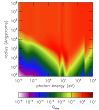
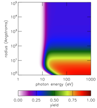
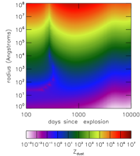
Figure 6: Grain properties as a function of grain radius and photon energy or time since the explosion, including: the absorption coefficient $Q_{\rm abs}$ (left panel), the photoelectric yield $Y$ for neutral ($Z=0$) carbon grains (middle panel), equilibrium grain charge $Z_{\rm dust}$ (right panel).

We follow Weingartner et al. (2006) and Draine & Sutin (1987) to find an expression for the rate at which electrons are ejected from a grain by photoelectric absorption. The general formula for the photoelectric ejection rate is:

$$\Gamma_{\gamma}=\int_{0}^{\infty}n_{\gamma}(E)Q_{\rm abs}(E,a)\pi a^{2}cY(E,a,Z)dE,$$ (39)

where $Y(E,a,Z)$ is the photoelectric yield, namely, the average number of electrons ejected from a grain of radius $a$ and charge $Ze$ when it absorbs a photon with energy $E$, and $Q_{\rm abs}(E,a)$ is the absorption coefficient defined such that the cross section for a grain to absorb a photon of energy $E$ is $\sigma_{\rm abs}(E,a)=Q_{\rm abs}(E,a)\pi a^{2}$. For the absorption coefficient of all grain species we used an online table based on Draine & Lee (1984) and Laor & Draine (1993). This table provides grain radius and photon energy dependent absorption coefficients for graphite spheres with radii $1\,\textrm{nm}\leq a\leq 10\,\textrm{$\mu$m}$. For smaller grains we assume that $Q_{\rm abs}(E,a)\propto a$ and for larger grains that $Q_{\rm abs}(E,a)$ is independent of radius. We plot the absorption coefficient as a function of the grain radius and photon energy in the left panel of Figure 6.

To find the yield for given $E$, $a$, and $Z$, we write the valence band ionization potential

$$I=W+\left(Z+\frac{1}{2}\right)\frac{e^{2}}{a}+(Z+2)\frac{e^{2}}{a}\frac{0.3\,\textrm{\AA}}{a},$$ (40)

where $W$ is the work function that we take to equal $W=4.4\,\textrm{eV}$ (Weingartner & Draine, 2001). The minimum energy an electron must have to escape a negatively charged grain is:

$$E_{\rm min}=\frac{e^{2}|Z+1|}{1+|Z+1|^{-1/2}}\left[1-\frac{0.3}{|Z+1|^{0.26}}\left(\frac{a}{10\,\textrm{\AA}}\right)^{-0.45}\right]$$ (41)

if $Z<-1$ and $E_{\rm min}=0$ otherwise. The threshold energy for photoelectric emission is $E_{\rm PET}=I+E_{\rm min}$ if $Z<1$ and $E_{\rm PET}=I$ otherwise. We define auxiliary quantities: $\Theta=E-E_{\rm PET}$ if $Z<0$ and $\Theta=E-E_{\rm PET}+(Z+1)e^{2}/a$ othrewise, $\alpha=a/l_{\rm a}+a/l_{\rm e}$, $\beta=a/l_{\rm a}$, where $l_{\rm a}$ is the photon attenuation length that we take to be $l_{\rm a}=27.8\,\textrm{\AA}$ and $l_{\rm e}$ is the electron escape length which we take to be $l_{\rm e}=10.0\,\textrm{\AA}$. We define further auxiliary quantities:

$$y_{0} = 0.009\times\frac{(\Theta/W)^{5}}{1+0.037(\Theta/W)^{5}},$$ (42)

$$y_{1} = \left(\frac{\beta}{\alpha}\right)^{2}\frac{\alpha^{2}-2\alpha+2-2e^{-\alpha}}{\beta^{2}-2\beta+2-2e^{-\beta}},$$ (43)

$$y_{2} = \begin{cases}\frac{E_{\rm high}^{2}(E_{\rm high}-3E_{\rm low})}{(E_{\rm high}-E_{\rm low})^{3}},&\mbox{ if }Z\geq 0,\\ 1,&\mbox{ if }Z<0,\end{cases}$$ (44)

as well as $E_{\rm high}=E_{\rm min}+E-E_{\rm PET}$ if $Z<0$ and $E_{\rm high}=E-E_{\rm PET}$ otherwise, $E_{\rm low}=E_{\rm min}$ if $Z<0$ and $E_{\rm low}=-(Z+1)e^{2}/a$ otherwise. The yield is non-zero when $E>E_{\rm PET}$ and equals $Y=y_{2}\times\mbox{min}\{\,y_{0}y_{1},\,1\,\}$. The photoelectric yield of a neutral carbon grain as a function of grain radius and photon energy is shown in Figure 6, middle panel.

The total time derivative of the electric charge of a grain is:

$$\frac{dZ}{dt}=-\Gamma_{e^{-}}+z_{\rm ion}\Gamma_{\rm ion}+\Gamma_{\gamma}.$$ (45)

The equilibrium charge is found by setting $dZ/dt=0$ and solving for $Z$. We assume that all grain species have the same grain-radius-dependent charge computed according to the just described procedure substituting the values of $Q_{\rm abs}$, $Y$, and $W$ specific to carbon grains. We set $T_{e}=T_{\rm ion}=T_{\rm gas}$, $z_{\rm ion}=+1$, $m_{\rm ion}=20.3\,\textrm{amu}$, and $c_{\rm ion}=c_{e}=2.94\times 10^{8}\,\textrm{cm}^{-3}(t/100\,\textrm{days})^{-3}$ in all calculations (including those pertaining to the bubble and ambient density regions). We plot the equilibrium grain charge $Z_{\text{dust}}$ in the right panel of Figure 6.

4.5 Grain temperature

The temperature of a dust grain can be different from the temperature of the gas and is an important parameter because the evaporation rate, as we discuss below, depends on the grain temperature exponentially. We explicitly compute the grain temperature as a function of grain radius. For the purpose of this calculation only, we assume the grain is pure carbon regardless of its actual composition. Dust grains heat by absorbing photons from the UV radiation field and cool by emitting IR photons. They also exchange energy with the surrounding gas via gas-grain collisions. We ignore the heating and cooling due to evaporation, accretion, coagulation, and chemical reactions.

The rate at which the internal energy $U$ of a grain with radius $a$ increases through absorption of UV photons is:

$$L_{\rm abs}(a)=\pi a^{2}c\int_{0}^{\infty}Q_{\rm abs}(E,a)En_{\gamma}(E)dE,$$ (46)

where $c$ is the speed of light. The rate at which a grain with temperature $T_{\rm dust}$ cools by emitting IR photons is:

$$L_{\rm emit}(a,T_{\text{dust}})=\frac{4\pi^{6}a^{2}{k_{\rm B}}T_{\rm dust}}{15h^{3}c^{2}\zeta(3)}\int_{0}^{\infty}\frac{E^{2}Q_{\rm abs}(E,a)}{e^{E/{k_{\rm B}}T_{\rm dust}}-1}dE,$$ (47)

where $h$ is Planck’s constant and $\zeta(x)$ is the Riemann-Zeta function. Collisions with gas particles effect energy transfer (heating or cooling) at the rate (Burke & Hollenbach, 1983):

$$L_{\rm gas}(a,T_{\text{gas}},T_{\text{dust}}) = \pi a^{2}n_{\rm tot}\sqrt{\frac{8{k_{\rm B}}T_{\rm gas}}{\pi\left\langle m\right\rangle}}$$ (48)

$$\times(0.1+0.35\,e^{-\sqrt{(T_{\rm dust}+T_{\rm gas})/500\>\rm K}})$$

$$\times 2{k_{\rm B}}(T_{\rm gas}-T_{\rm dust}).$$

The equilibrium grain temperature is found by setting

$$L_{\rm abs}(a)-L_{\rm emit}(a,T_{\text{dust}})+L_{\rm gas}(a,T_{\text{gas}},T_{\text{dust}})=0$$ (49)

and solving for $T_{\rm dust}$.

For the gas density we use $n_{\rm tot}=2.23\times 10^{11}\,\textrm{cm}^{-3}(t/100\,\textrm{days})^{-3}$ and for average gas particle mass we use $\left\langle m\right\rangle=3.07\times 10^{-23}\,\textrm{g}$. These are valid in the bubble shells but we also use them for ambient and nickel bubble regions. Fixing the gas density here to the density in the shells is justified by noting that in the period $100$–$1000$ days after the explosion when the dust forms, the collisional gas-dust coupling is negligible compared to the dust’s thermal coupling to radiation. E.g., for small $1\,\text{nm}$ grains we have $L_{\text{abs}}\gtrsim 100\times L_{\text{gas}}$. Therefore the dust temperature is not sensitive to gas density. In Figure 8 we plot grain temperature as a function of time and grain radius.

Figure 7: Evaporation suppression factor (left panel) and evaporation rate (right panel) as a function of grain radius and temperature.

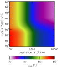
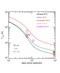
Figure 8: Grain temperature as a function of time and grain radius (left panel) and measured values dust temperature (right panel) from Dwek & Arendt (2015) (DA15) and Wesson et al. (2015) (W15), where in the right panel, the solid lines are solutions of Equation (49).

4.6 Evaporation

Atoms at the surface of a dust grain can be ejected into the gas phase in a process called evaporation (or sublimation). To calculate the evaporation rate as a function of radius and grain temperature we follow Guhathakurta & Draine (1989) and idealize a grain as consisting of $N$ atoms, each connected to the lattice with a spring. Each atom can vibrate in three independent directions so the grain has $3N$ degrees of freedom. Since 6 of these correspond to translation and rotation of the grain as a whole, the grain has $F=3N-6$ vibrational degrees of freedom. The internal or thermal energy $U$ of the grain is distributed over these vibrational degrees of freedom.

We assume that each grain species behaves as an Einstein solid with Debye temperature $T_{\text{D}}$. The vibrational degrees of freedom are treated as quantum harmonic oscillators with angular frequency $\omega_{0}=(\pi/6)^{1/3}{k_{\rm B}}T_{\text{D}}/\hbar$. The total number of vibrational quanta in a grain is $U/\hbar\omega_{0}$ and the average number of quanta per vibrational degree of freedom is $\gamma=U/\hbar\omega_{0}F$. The values of $T_{\text{D}}$ used in our simulation are given in Table 8.

The number of quanta in a vibrational degree of freedom fluctuates as energy shifts between atoms in a grain. Every once in a while, one vibrational degree of freedom has so much energy that the atom becomes unbound and is ejected from the grain. The surface binding energy of the atom to the grain of radius $a$ and surface tension $\sigma_{\text{ST}}$ is:

$$\mathcal{E}_{\rm bind}={k_{\rm B}}A-4\pi r_{1}^{2}\sigma_{\text{ST}}[(n-1)^{2/3}-(n-2)^{2/3}],$$ (50)

where $A$ is the bulk binding energy of an atom to the grain divided by the Boltzmann constant. Then, for evaporation to occur, the number of quanta that must be concentrated in a single vibrational degree of freedom is $b=\mathcal{E}_{\rm bind}/\hbar\omega_{0}$.

For single-element grains evaporation is the process:

$$\mathcal{X}_{n}\to\mathcal{X}_{n-1}+\mathcal{X}.$$ (51)

This occurs at a rate per unit volume $k_{\rm evap}(T,n)c_{n}$, where, in the limit in which the grains are in thermal equilibrium with the gas, the evaporation rate coefficient is:

$$k_{\rm evap}(T,n) = p_{\rm s}s_{n}a_{n}^{2}\sqrt{\frac{8\pi}{{k_{\rm B}}Tm_{1}}}e^{-\mathcal{E}_{\text{bind}}/{k_{\rm B}}T+B}.$$ (52)

Here $p_{\rm s}=10^{6}\,\textrm{dyne}\,\textrm{cm}^{-2}$ is the standard pressure, $s_{n}$ is the sticking coefficient (which we take to be unity), and $B$ is a parameter that depends on the grain composition (i.e., the species). This expression was derived by setting the evaporation rate equal to the condensation rate when the partial pressure equals the vapor pressure (Nozawa & Kozasa, 2013). The values of the parameters $A$, $B$, $\sigma_{\text{ST}}$, and $r_{1}$ that we use can be found in Table 7.

In reality, grains may not be in thermal equilibrium with the gas. The gas density can be so low that thermal fluctuations within a grain occur much faster than the grain exchanges energy with the the ambient atoms and molecules. Therefore, the energy needed to remove an atom from a grain may have to come from a thermal fluctuation within the grain itself. We can account for this thermal isolation by multiplying the evaporation rate coefficient with a dimensionless suppression factor $S_{N}$. The suppression factor is the ratio of the actual probability that there will be at least $b$ quanta in one vibrational degree of freedom to what that probability would be if the grain were in thermal equilibrium with the gas. The probability that there is at least $b$ quanta in one vibrational degree of freedom is (Guhathakurta & Draine, 1989):

$$\tilde{p}_{F}(\gamma,b)=\frac{(\gamma F)!(\gamma F-b+F-1)!}{(\gamma F+F-1)!(\gamma F-b)!}.$$ (53)

The same probability if the grain were coupled to a heat bath and thus $F\to\infty$ would be:

$$\tilde{p}_{\infty}(\gamma,b)=\left(\frac{\gamma}{1+\gamma}\right)^{b}.$$ (54)

Dividing Equation (53) with (54) gives the suppression factor (Guhathakurta & Draine, 1989):

$$S_{N}(T_{\rm dust}) = \frac{\tilde{p}_{F}(\gamma,b)}{\tilde{p}_{\infty}(\gamma,b)}$$ (55)

$$= \left(\frac{1+\gamma}{\gamma}\right)^{b}\frac{(\gamma F)!(\gamma F-b+F-1)!}{(\gamma F+F-1)!(\gamma F-b)!}.$$

Note that if $\gamma F<b$, there is not enough internal energy in the grain for evaporation and the suppression factor (and thus the evaporation rate) should be set to zero.

We discretize the evaporation process on the grid of grain radii:

$$\mathcal{Z}_{\ell}\to\mathcal{Z}_{\ell-1}+\delta n_{\ell-1}\mathcal{X},$$ (56)

where

$$\delta n_{\ell-1}=\left(\frac{a_{\ell}}{a_{1}}\right)^{3}-\left(\frac{a_{\ell-1}}{a_{1}}\right)^{3}$$ (57)

is the number of monomers that would need to be added to an $(i-1)$mer to obtain an $i$mer. The rate per unit volume of the reaction in Equation (56) is:

$$\mathcal{R}^{\rm evap}_{\ell}=\frac{k_{\rm evap}(T_{\rm dust},n_{\ell})S_{N}(T_{\rm dust})c_{\ell}}{\delta n_{\ell-1}}.$$ (58)

We turn to multi-element grains which evaporate by losing atoms as well as molecules via the reaction:

$$\mathcal{Z}_{\ell}\to\mathcal{Z}_{\ell-1}+\delta n_{\ell-1}(\nu_{1}\mathcal{A}_{1}+...+\nu_{N}\mathcal{A}_{N}),$$ (59)

where $\mathcal{A}_{i}$ denote molecular species. Table 8 gives the coefficients of evaporative reactions for all grain species. We assume that the evaporation rate, in monomers per unit time, can be approximated with Equation (52), but now with ‘$n$’ interpreted as the number of monomers in the grain. The parameters needed to calculate the evaporation rate of a multi-element grain can also be found in Table 7–8. The suppression factor and evaporation rate for carbon grains are plotted in Figure 7.

The change of molecular abundances due to grain evaporation is given by:

$$\left(\frac{dc_{\mathcal{A}_{k}}}{dt}\right)_{\rm evap} = \nu_{k}\sum_{\ell=1}^{\ell_{\rm max}}\delta n_{\ell-1}\mathcal{R}^{\rm evap}_{\ell}$$ (60)

and the corresponding change of grain abundances is given by:

$$\left(\frac{dc_{\ell}}{dt}\right)_{\rm evap} = \mathcal{R}^{\rm evap}_{\ell+1}-\mathcal{R}^{\rm evap}_{\ell}.$$ (61)

4.7 Accretion

Accretion is the inverse process of evaporation in which sub-monomeric fragments (or molecular monomer precursors; e.g., Mg, O, or SiO for a forsterite Mg₂SiO₄ grain) collide with and are absorbed by a grain. Suppose that accretion can be parametrized by stoichiometric coefficients $\nu_{1}$, …, $\nu_{N}$:

$$\mathcal{X}_{n}+\nu_{1}\mathcal{A}_{1}+...+\nu_{N}\mathcal{A}_{N}\to\mathcal{X}_{n+1}.$$ (62)

Each molecular species $\mathcal{A}_{i}$ collides with the grain at a rate $a^{2}c_{\mathcal{A}_{i}}\sqrt{8\pi{k_{\rm B}}T/m_{\mathcal{A}_{i}}}$. We define the key species as the one with the lowest collision rate. The rate at which monomers are accreted to the grain is:

$$k_{\rm acc}=\frac{a^{2}c_{\rm key}}{\nu_{\rm key}}\sqrt{\frac{8\pi{k_{\rm B}}T}{m_{\rm key}}}.$$ (63)

where the subscript ‘key’ designates the quantities associated with the key species. Discretizing this on the grid of grain radii we obtain the reaction:

$$\mathcal{Z}_{\ell}+\delta n_{\ell}(\nu_{1}\mathcal{A}_{1}+...+\nu_{N}\mathcal{A}_{N})\to\mathcal{Z}_{\ell+1}.$$ (64)

This reaction occurs at a rate per unit volume:

$$\mathcal{R}^{\rm acc}_{\ell} = \frac{k_{\rm acc}c_{\ell}}{\delta n_{\ell}}.$$ (65)

The change of molecular abundances due to accretion is given by:

$$\left(\frac{dc_{\mathcal{A}_{k}}}{dt}\right)_{\rm acc} = -\nu_{k}\sum_{\ell=1}^{\ell_{\rm max}}\delta n_{\ell}\mathcal{R}^{\rm acc}_{\ell}$$ (66)

and the corresponding change of grain abundances is given by:

$$\left(\frac{dc_{\ell}}{dt}\right)_{\rm acc} = \mathcal{R}^{\rm acc}_{\ell-1}-\mathcal{R}^{\rm acc}_{\ell}.$$ (67)

4.8 Weathering

Chemical weathering refers to the process in which atoms (and ions) in the gas phase collide with a grain and chemically react with an atom in the grain resulting in the removal of the latter atom from the grain. Like evaporation, chemical weathering is a grain destruction process. A prominent form of weathering is by noble gas ions. When an He⁺ ion collides with a grain it can steal an electron to recombine. The recombination energy goes into the grain and can result the ejection of an atom from the grain. In single element grains this corresponds to the reaction:

$$\mathcal{X}_{n}+\mbox{He}^{+}\to\mathcal{X}_{n-1}+\mathcal{X}^{+}+\mbox{He}.$$ (68)

We take the rate per unit volume of this reaction to be $k_{\rm He}c_{\rm He^{+}}c_{n}$, where the coefficient is (Lazzati & Heger, 2016):

$$k_{\rm He}=1.6\times 10^{-9}\,\textrm{cm}^{3}\,\textrm{s}^{-1}\times n^{2/3}.$$ (69)

This value is for carbon grains but we adopt it for all single-element grains.

For multi-element grains we assume that He⁺ ions collide with grains and remove one atom at a time at the same rate as in single element grains. More precisely, let (X₁)${}_{\eta_{1}}$(X₂)${}_{\eta_{2}}$(X₃)${}_{\eta_{3}}$ be the chemical formula for the monomer of some grain species, where X_k is the $k$th element and $\eta_{k}$ the number of atoms of that element. Then helium weathering corresponds to the reaction:

$$\mathcal{Z}_{\ell}+\delta n_{\ell-1}\eta_{0}\mbox{He}^{+}$$

$$\to\mathcal{Z}_{\ell-1}+\delta n_{\ell-1}\left(\eta_{1}\mbox{X}_{1}^{+}+\eta_{2}\mbox{X}_{2}^{+}+\eta_{3}\mbox{X}_{3}^{+}+\eta_{0}\mbox{He}\right)$$ (70)

with rate per unit volume:

$$\mathcal{R}^{\rm weath,He}_{\ell}=\frac{1}{\delta n_{\ell-1}\eta_{0}}\mathcal{K}_{0}\left(\frac{a_{\ell}}{a_{0}}\right)^{2}c_{\ell}c_{\rm He^{+}},$$ (71)

where $\mathcal{K}_{0}=1.6\times 10^{-9}\,\textrm{cm}^{3}\,\textrm{s}^{-1}$ and $\eta_{0}=\eta_{1}+\eta_{2}+\eta_{3}$. The time derivatives of the number densities of the affected species are:

$$\left(\frac{dc_{\rm He^{+}}}{dt}\right)_{\rm weath} = -\sum_{\ell=1}^{\ell_{\rm max}}\delta n_{\ell-1}\eta_{0}\mathcal{R}^{\rm weath,He}_{\ell}$$

$$= -\left(\frac{dc_{\rm He}}{dt}\right)_{\rm weath},$$

$$\left(\frac{dc_{\rm X_{k}}}{dt}\right)_{\rm weath} = \eta_{k}\sum_{\ell=1}^{\ell_{\rm max}}\delta n_{\ell-1}\mathcal{R}^{\rm weath,He}_{\ell},$$

$$\left(\frac{dc_{\ell}}{dt}\right)_{\rm weath,He} = \mathcal{R}^{\rm weath,He}_{\ell+1}-\mathcal{R}^{\rm weath,He}_{\ell}.$$ (72)

In principle, Ne⁺ and Ar⁺ can also contribute to weathering. We assume that this occurs with the same rate coefficient as for helium.

When a neutral oxygen atom collides with a carbon grain it can remove a carbon atom and form a CO molecule that is ejected into the gas phase. This corresponds to the reaction:

$$\mbox{C}_{n}+\mbox{O}\to\mbox{C}_{n-1}+\mbox{CO}.$$ (73)

We take the rate of this reaction from Lazzati & Heger (2016):

$$k_{\text{O}}=10^{-11}e^{-1130.0\>\rm K\it/T}n^{2/3}\,\textrm{cm}^{3}\,\textrm{s}^{-1}.$$ (74)

We only include this process, which is called oxygen weathering, for carbon grains.

Oxygen weathering is discretized on the grid of grain radii as follows. The effective reaction on grain radial grid points is

$$\mathcal{Z}_{\ell}+\delta n_{\ell-1}\mbox{O}\to\mathcal{Z}_{\ell-1}+\delta n_{\ell-1}\mbox{CO}$$ (75)

This occurs at a rate per unit volume of

$$\mathcal{R}_{\ell}^{\rm weath,O}=\frac{k_{\text{O}}c_{\ell}c_{\rm O}}{\delta n_{\ell-1}}$$ (76)

and affects the number density time derivatives as follows:

$$\left(\frac{dc_{\rm O}}{dt}\right)_{\rm weath} = -\delta n_{\ell-1}\mathcal{R}_{\ell}^{\rm weath,O},$$

$$\left(\frac{dc_{\rm CO}}{dt}\right)_{\rm weath} = \delta n_{\ell-1}\mathcal{R}_{\ell}^{\rm weath,O},$$

$$\left(\frac{dc_{\ell}}{dt}\right)_{\rm weath,O} = R_{\ell+1}^{\rm weath,O}-\mathcal{R}_{\ell}^{\rm weath,O}.$$ (77)

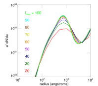
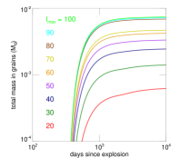
Figure 9: The curves show the final size distribution (left) and grain mass versus time (right) of carbon grains from a series of test simulations in which all parameters were held fixed except for the number of radial grid points $\ell_{\rm max}$. The upturn in $a^{4}dN/da$ at grain sizes $a\gtrsim 0.3\,\mu\text{m}$ is a numerical artifact resulting from the finite extent of the radial grid.

5 Time integration

In our time integration calculation, an ejecta fluid element is described by a state vector of dimension $\mathcal{N}=\mathcal{N}_{\text{S}}+\mathcal{N}_{\text{G}}\times\ell_{\rm max}=95+14\times 50=795$. We track $\mathcal{N}_{\text{R}}=341$ chemical reactions that modify the state vector and solve $\mathcal{N}$ coupled ordinary differential equations (ODEs) of the form

$$\frac{dc_{i}}{dt} = \left(\frac{dc_{i}}{dt}\right)_{\text{chem}}+\left(\frac{dc_{i}}{dt}\right)_{\text{Compt}}+\left(\frac{dc_{i}}{dt}\right)_{\text{coag}}$$ (78)

$$+ \left(\frac{dc_{i}}{dt}\right)_{\text{evap}}+\left(\frac{dc_{i}}{dt}\right)_{\text{acc}}+\left(\frac{dc_{i}}{dt}\right)_{\text{weath}}-3\frac{c_{i}}{t}.$$

Here, $(dc_{i}/dt)_{\text{chem}}$ is from Equation (14), $(dc_{i}/dt)_{\text{Compt}}$ is from Equations (21) and (3.3), $(dc_{i}/dt)_{\text{coag}}$ is from Equation (29), $(dc_{i}/dt)_{\text{evap}}$ is from Equations (60) and (61), $(dc_{i}/dt)_{\text{acc}}$ is from Equations (66) and (67), $(dc_{i}/dt)_{\text{weath}}$ is from Equations (4.8) and (4.8), and the last term on the right is the overall decrease of number density due to homologous expansion. The ODEs are integrated with a Bulirsch-Stoer-type, semi-implicit extrapolation mid-point method (Bader & Deuflhard, 1983).

Our science suite of consists of 108 integrations, specifically 8, 50, and 50 integrations in the nickel bubbles, ambient ejecta, and dense shells, respectively. The integrations covered mass coordinate ranges $1.82M_{\odot}<M<1.89M_{\odot}$ in the nickel bubbles and $1.89M_{\odot}<M<6.81M_{\odot}$ for the ambient ejecta and dense shells. Each integration was started at 100 days after the explosion and carried out until a post-explosion time of $10^{4}\,\text{d}$. Since at $10^{4}\,\text{d}$, the specific dust formation rate is $|d\ln M_{\rm dust,tot}/dt|^{-1}\sim 4000\,\textrm{years}$, no significant dust growth is expected at still later times.

The density in the shells depends on their thickness relative to the bubble radius. This thickness is not constrained by observations and one should vary the shell thickness as a parameter. We found very overdense shell integrations too computationally expensive, and thus, simulated shells only as dense as four times the ambient ejecta density. Specifically, we ran the shell integrations at three different densities, 1, 2, and 4 times the density in the ambient ejecta.

5.1 Convergence test

We performed a convergence test by running a suite of integrations that are identical except for the number of radial mesh points $\ell_{\rm max}$. In the test, the density was set to the ambient ejecta density, the temperature was set to the atomic temperature evolution track (Figure 3, right panel), the mass fraction of C was set to 0.3, the mass fractions of He, O, Mg, Al, Si, S, and Fe were set to 0.1.

The left panel of Figure 9 shows the carbon grain size distribution in the form $a^{4}dN/da$ at the end of the simulations, $10^{4}$ days after the explosion. The maximum fractional residual

$$\max_{\ell}\frac{|(dN/da)_{\ell}^{(\ell_{\rm max})}-(dN/da)_{\ell}^{(\ell_{\rm max}=100)}|}{(dN/da)_{\ell}^{(\ell_{\rm max}=100)}}$$ (79)

in the interesting range of grain radii $10\,\textrm{\AA}\leq a<1\,\textrm{$\mu$m}$ decreases monotonically in $\ell_{\rm max}$ and drops to $\approx 0.5$ for the resolution we adopt, $\ell_{\rm max}=50$; the average residual is much smaller. The location of the peak of $a^{4}dN/da$ is accurate independent of $\ell_{\rm max}$.

The right panel of Figure 9 shows the mass in carbon grains as a function of time. The maximum fractional residual in the final carbon grain mass drops to $\approx 0.5$ for $\ell_{\rm max}=50$. The fractional residual in the CO number density at the end of the simulation, not shown, drops below $0.01$ for the same number of grid points.

6 Results

The model described in the preceding sections can be applied to arbitrary core collapse supernovae. The specific objective of the numerical integrations we present here is to assess the efficiency of dust production in SN 1987A. From each integration we derive the dust mass synthesized as a function of grain composition and size. Different integrations sample the various chemically and hydrodynamically distinct zones.

Our presentation of the results is structured as follows. We first analyze how dust mass is partitioned as a function of grain size and composition and how refractory element mass is partitioned between molecules and grains of different sizes. Then we examine the evolution of grain mass by species, ejecta zone, and mass coordinate within the ejecta. We analyze the shape of the grain size (or, equivalently, grain mass) distribution at $10^{4}$ days. Next we turn the evolution of the abundance of important molecules and how their abundances are distributed throughout the ejecta. Finally, we discuss how the grain properties depend on the mass density in the dense shells compressed by nickel bubbles.

Species	Very Small	Small	Medium	Large	Very Large	Giant	Total
Alumina	0	3.5($-$7)	1.2($-$2)	7.5($-$4)	1.8($-$10)	4.0($-$7)	1.4($-$2)
Carbon	1.5($-$10)	4.7($-$7)	1.9($-$3)	2.2($-$2)	8.8($-$3)	1.0($-$3)	3.4($-$2)
Enstatite	0	3.8($-$7)	2.8($-$5)	1.3($-$6)	0	0	3.0($-$5)
Forsterite	0	2.0($-$5)	8.9($-$2)	6.0($-$3)	2.1($-$10)	4.2($-$7)	0.1
Iron	1.2($-$8)	3.0($-$5)	4.1($-$3)	2.5($-$3)	9.3($-$6)	0	6.6($-$3)
Iron Oxide	0	1.7($-$10)	3.7($-$6)	1.5($-$4)	6.4($-$9)	0	1.5($-$4)
Iron Sulfide	0	7.3($-$6)	1.3($-$2)	2.7($-$2)	2.0($-$3)	0	4.1($-$2)
Magnesia	8.0($-$10)	1.1($-$3)	0.13	4.6($-$2)	9.7($-$10)	0	0.17
Magnetite	0	0	3.5($-$7)	2.7($-$4)	3.3($-$7)	0	2.6($-$4)
Silicon Carbide	0	0	0	0	0	1.8($-$7)	1.8($-$7)
Silicon Dioxide	7.3($-$9)	6.6($-$3)	1.7($-$2)	3.0($-$7)	0	0	2.0($-$2)
Silicon	9.8($-$9)	4.4($-$4)	6.4($-$2)	5.7($-$3)	8.9($-$2)	1.2($-$3)	0.16
Total	3.0($-$8)	8.8($-$3)	0.31	0.11	9.9($-$2)	2.2($-$3)	0.59

Table 9: Final dust mass classified by grain species and size for ($a<1\,\textrm{nm}$), small ($1\,\textrm{nm}\leq a<10\,\textrm{nm}$), medium ($10\,\textrm{nm}\leq a<0.1\,\textrm{$\mu$m}$), large ($0.1\,\textrm{$\mu$m}\leq a<1\,\textrm{$\mu$m}$), very large ($1\,\textrm{$\mu$m}\leq a<10\,\textrm{$\mu$m}$), and giant ($a\geq 10\,\textrm{$\mu$m}$) grains.

6.1 Grains

Figure 8 shows the dust temperature as a function of time and grain radius. At a given radius the temperature drops rapidly with time. For example, the temperature of $1\,\text{nm}$ grains is $\sim 4500\,\text{K}$ at $100$ days; it drops to $\sim 350\,\text{K}$ at $1000$ days and further to $\sim 70\,\text{K}$ at $10^{4}$ days. The temperature of grains with radii above a micron starts at $\sim 2000\,\text{K}$ at $100$ days and already drops to $\sim 60\,\text{K}$ by $1000$ days. At $10^{4}$ days the dust temperature is $\lesssim 20\,\text{K}$ which is consistent with the dust temperature inferred by Zanardo et al. (2014) from observations with Australia Telescope Compact Array (ATCA) and ALMA. The impact of the dust temperature on the evaporation rate can seen in the right panel of Figure 7. The evaporation rate, which depends on the dust temperature, drops quickly to become completely negligible after $300$ days. The rate of accretion onto grains, which depends on the higher gas temperature, does not drop as fast. Therefore, after $300$ days, grain growth proceeds unimpeded by evaporation and is only modulated by noble gas weathering.

In Table 9 we provide the dust mass synthesized a function of grain size for each of the grain species. At the end of the simulation the total dust mass produced was $\approx 0.5\,M_{\odot}$, the bulk of which, $\approx 0.3\,M_{\odot}$, was in medium size grains ($10\,\text{nm}\leq a<100\,\text{nm}$), and another $\approx 0.1\,M_{\odot}$ each in large ($0.1\,\mu\text{m}\leq a<1\,\mu\text{m}$) and very large ($1\,\mu\text{m}\leq a<10\,\mu\text{m}$) grains.

Species	1	2	3	4	$5+$	Small	Medium	Large	Very Large	Giant
Carbon	0.13	2.6($-$2)	0	0	0	3.4($-$7)	1.2($-$3)	1.4($-$2)	3.4($-$3)	3.9($-$4)
Iron	5.9($-$2)	1.0($-$4)	1.8($-$8)	0	0	8.1($-$6)	4.5($-$3)	3.9($-$3)	1.9($-$4)	0
Magnesium	3.5($-$3)	3.1($-$4)	0	0	0	4.5($-$4)	7.5($-$2)	2.3($-$2)	5.1($-$10)	1.1($-$7)
Oxygen	2.0	3.9($-$2)	8.1($-$8)	0	1.7($-$5)	3.1($-$3)	7.2($-$2)	1.5($-$2)	1.7($-$8)	2.6($-$7)
Sulfur	0.15	4.7($-$5)	0	0	0	1.2($-$6)	2.2($-$3)	1.9($-$3)	1.0($-$4)	0
Silicon	0.17	2.8($-$4)	1.5($-$7)	0	2.7($-$5)	2.4($-$3)	4.2($-$2)	2.6($-$3)	3.9($-$2)	7.6($-$4)
Aluminum	4.1($-$3)	9.8($-$6)	0	0	0	1.4($-$7)	4.5($-$3)	2.9($-$4)	0	1.5($-$7)

Table 10: Ejecta mass in solar masses by element and number of atoms or grain size in the same grain size bins as in Table 9.

Table 10 provides the partitioning of the elemental mass into different chemical products. Overall, the simulated ejecta contains noble gases (He, Ne, and Ar) and refractory elements (C, O, Mg, Al, Si, S, and Fe). In the simulation the noble gases comprise $1.8\,M_{\odot}$ or $37\%$ of the core mass, whereas the refractory elements, which can be incorporated in grains, comprise $3.1\,M_{\odot}$ or $62\%$. Approximately $16\%$ of this refractory mass has ended up in grains at $10^{4}$ days. The rest of the refractory mass remained in atomic form ($2.5\,M_{\odot}$ or 82%) with a small fraction locked in molecules, predominantly diatomic ($0.069\,M_{\odot}$ or 2%).

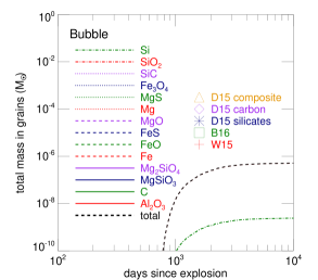
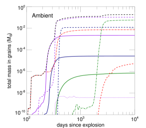
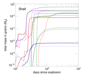
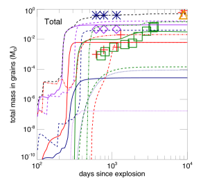
Figure 10: The curves show the evolution of dust mass in the nickel bubbles (upper left), ambient ejecta (upper right), and thin shells at the bubble-ambient interface (lower left), and the sum of the three (lower right). Observations of dust mass in SN 1987A are shown as green squares (Bevan & Barlow, 2016) and blue crosses (Wesson et al., 2015). The solid magenta line is a power law fit to the observations. The solid dashed line is the total dust mass summed over all grain species.

In Figure 10 we plot the evolution of the dust mass in each of the three ejecta zones: the nickel bubbles, the ambient ejecta, and the dense shells at the bubble and ambient ejecta interface. The total dust mass in all zones and the observations from Bevan & Barlow (2016), Wesson et al. (2015), and Dwek & Arendt (2015) are also shown on the lower right panel; we compare the computed and observationally inferred masses in Section 7.2 below.

Dust formation is rapid between 215 and 620 days after the explosion. The average dust growth rate is $\sim 0.3\,M_{\odot}\,\textrm{yr}^{-1}$. After 620 days, dust formation continues at a much slower rate $\sim 0.006\,M_{\odot}\,\textrm{yr}^{-1}$. There are actually five distinct epochs when the dust growth rate $dM_{\rm dust}/dt$ spikes. Peak dust formation rate, mostly due to the formation in shells, occurs at 229 days for forsterite, 332 days for magnesia, 382 days for iron sulfide, 528 days for silicon, and 2551 days for carbon. The overall dust formation rate peaks at $dM_{\rm dust}/dt\approx 1\,M_{\odot}\,\textrm{yr}^{-1}$ at 332 days.

Most of the dust forms in the dense shells ($0.32\,M_{\odot}$ or 63% of the total mass). Less forms in the ambient ejecta ($0.18\,M_{\odot}$ or 37%), and very little in the bubbles ($5\times 10^{-7}\,M_{\odot}$). This reflects the strong density dependence of dust yield: the nucleation rate is proportional to the square of the number density $(dc_{i}/dt)_{\text{nuc}}\propto c_{1}^{2}$ and the accretion rate is proportional to the density $(dc_{i}/dt)_{\text{acc}}\propto c_{1}$. It is also because at high densities the ionization fraction, and thus the weathering rate, is lower.

Not only the grain mass produced but also its chemical composition differs between the ambient and shell zones. Carbon and iron grains have a significantly higher mass in dense shells than in ambient ejecta. Alumina, iron oxide, and magnetite grains do not form at all in the ambient ejecta but do form in significant amounts in the dense shells. All other grain species are produced in similar quantities in the ambient ejecta and shells.

Species	Bubble	Ambient	Shell	Total
Alumina	0	0	6.1($-$3)	6.1($-$3)
Carbon	0	7.6($-$7)	3.0($-$2)	3.0($-$2)
Enstatite	0	2.7($-$5)	5.7($-$7)	2.6($-$5)
Forsterite	0	2.0($-$3)	9.0($-$2)	9.0($-$2)
Iron	5.0($-$7)	5.0($-$6)	5.8($-$3)	6.4($-$3)
Iron Oxide	0	0	1.4($-$4)	1.4($-$4)
Iron Sulfide	0	1.2($-$2)	2.6($-$2)	3.8($-$2)
Magnesia	0	0.1	5.6($-$2)	0.16
Magnetite	0	0	8.5($-$5)	8.5($-$5)
Silicon Carbide	0	3.7($-$9)	1.7($-$7)	1.7($-$7)
Silicon Dioxide	0	7.8($-$3)	1.4($-$2)	2.2($-$2)
Silicon	2.6($-$9)	5.6($-$2)	9.5($-$2)	0.15
Total	5.0($-$7)	0.19	0.33	0.51

Table 11: The same as Table 9, but now providing the final dust mass classified by grain species as well as the ejecta zone.

Table 11 provides the dust yield classified by grain species. The eight most abundant grain species are: magnesia ($0.16\,M_{\odot}$ or 32% of the total dust mass), silicon ($0.15\,M_{\odot}$ or 29%), forsterite ($0.092\,M_{\odot}$ or 18.0%), iron sulfide ($0.04\,M_{\odot}$ or 7.78%), carbon ($0.031\,M_{\odot}$ or 6.1%), silicon dioxide ($0.021\,M_{\odot}$ or 4%), alumina ($0.013\,M_{\odot}$ or 2.4%), and iron ($0.0062\,M_{\odot}$ or 1.2%).

A variety of competing effects influences the evolution of the mass in a grain species. At the earliest times grains are hot and evaporation completely inhibits grain growth. As the grain temperature drops, the evaporation rate decreases exponentially, and at some point it becomes negligible. Then, chemical weathering becomes the main grain destruction process. But even this is progressively less significant as the ionized fraction gradually decreases (it never becomes completely negligible). Dust formation ceases when the accretion time exceeds the expansion time. Coagulation does not affect the total dust mass although it modifies the size distribution. However, the coagulation rate is always lower than the accretion rate because the abundance of material in clusters that can accrete onto a grain is always higher that in other grains.

The sudden rise of carbon dust mass at $\sim 2000$ days is due to grain formation in the dense shells located in the mass coordinate range $4.5$–$7\,M_{\odot}$. There, the bulk of the mass is in helium and the abundance of He⁺ is very high. For example, at the mass coordinate $5.7\,M_{\odot}$ we find that the He⁺ relative abundance is $10\%$ at 100 days and 0.06% at 1000 days. At 1830 days the He⁺ abundance reaches a minimum of 0.04% and thereafter increases steadily to 0.2% at $10^{4}$ days. Thus, $\sim 2000$ days is when the He⁺ weathering is at a relative minimum and this is the optimal time to produce carbon dust. The carbon dust mass increase between 300 and 400 days seen in Figure 10 occurs at mass coordinate $\sim 4.8\,M_{\odot}$ where the abundance of carbon exceeds that of helium and thus helium weathering is not an obstacle. Carbon is substantially more abundant than helium between $2\,M_{\odot}$ and $5\,M_{\odot}$, but inwards of $4.5\,M_{\odot}$, carbon dust formation is poor due to decreasing carbon mass fraction, the presence of the two other noble gas ions, Ne⁺ and Ar⁺, and an increasing oxygen abundance and thus stronger oxygen weathering.

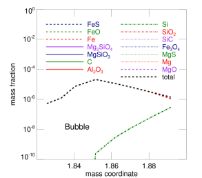
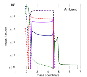
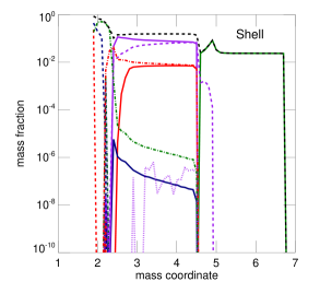
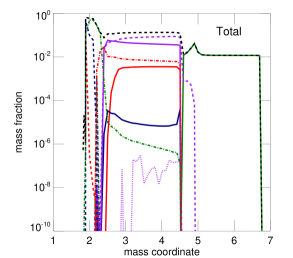
Figure 11: Grain mass fraction as a function of the mass coordinate in bubbles (upper left), ambient ejecta (upper right), dense shells (lower left), and all zones combined (lower right).

Figure 11 shows the mass fraction in each of the grain species as a function of the mass coordinate within the ejecta at the end of the simulation. The low-density bubbles form only a very small amount of silicon and iron grains with a total depletion fraction of $10^{-7}$–$10^{-5}$. In the ambient ejecta grains form in significant amounts for $M<4.5\,M_{\odot}$. Specifically, silicon and iron sulfide dominate the grain mass fraction for $M<2.25\,M_{\odot}$, and some iron grains are present there as well. For $2.25\,M_{\odot}<M<4.5\,M_{\odot}$, magnesia is the dominant grain species, followed by silicon dioxide, forsterite, and enstatite. In the carbon-rich region $4.5\,M_{\odot}<M<5\,M_{\odot}$ some carbon grains manage to form, comprising only a small mass fraction ($\sim 10^{-6}$–$10^{-5}$). Grains are practically absent in the helium rich outer core $M>5\,M_{\odot}$.

The shell ejecta produce the highest diversity of grain species. The innermost region ($M<2.25\,M_{\odot}$) again forms silicon, iron sulfide, and iron grains. The next region ($2.25\,M_{\odot}<M<4.5\,M_{\odot}$) forms, in decreasing order of yield: forsterite, magnesia, silicon dioxide, alumina, silicon, silicon carbide, and enstatite. The carbon-rich region $4.5\,M_{\odot}<M<5\,M_{\odot}$ froms carbon and magnesia grains. The outermost helium core $M>5\,M_{\odot}$ forms only carbon grains. In the entire ejecta carbon grains only form when $M>4.5\,M_{\odot}$ and they mostly form in the dense shells.

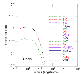
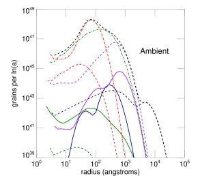
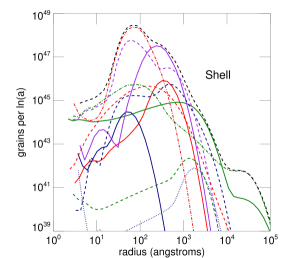
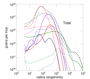
Figure 12: The curves show the grain size distribution $dN_{\text{dust},p}/d\ln a$ at the end of the simulation in the nickel bubbles (upper left), ambient ejecta (upper right), and thin shells at the bubble-ambient interface (middle left), and combined across the three zones (middle right).

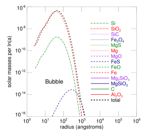
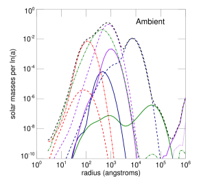
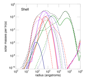
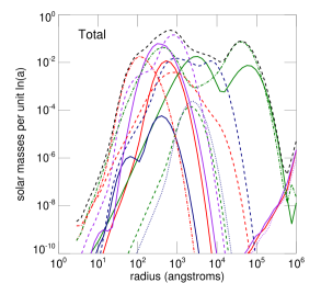
Figure 13: The same as Figure 12, but now showing the dust mass per logarithm of the radius $dM_{{\rm dust},p}/d\ln a$.

Figure 12 shows the logarithmic size distribution (grains per log grain radius) at the end of the simulation. The distribution peaks at $5.3\,\textrm{\AA}$ in the bubbles and $66\,\textrm{\AA}$ in the ambient ejecta, shells, and overall ejecta. We also plot the mass in grains per unit logarithmic radius $dM_{{\rm dust},p}/d\ln a$ at the end of the simulation in Figure 13. This distribution peaks at $50.5\,\textrm{\AA}$, $682\,\textrm{\AA}$, $526\,\textrm{\AA}$, and $682\,\textrm{\AA}$ in the bubbles, ambient ejecta, shells, and total ejecta, respectively. The total grain size distribution beyond the peak is approximately a power law:

$$\frac{dN}{d\ln a}\propto a^{-3.4}.$$ (80)

This is steeper than the classical grain size distribution in the ISM, $dN/d\ln a\propto a^{-2.5}$ (Mathis et al., 1977). The sharp rise of $dM_{{\rm dust},p}/d\ln a$ with radius at the largest radii, $a\gtrsim 10\,\mu\text{m}$, is an artifact of a numerical instability of our time primitive discretization scheme.

6.2 Molecules

The molecules CO, SiO, SO, and O₂ play important roles in dust formation. CO locks up carbon atoms so they cannot be added to carbon and silicon carbide grains. SiO is required to form the condensation nuclei of enstatite, forsterite, and silicon dioxide, whereas SO and O₂ are oxidizing agents that play a role in the formation of enstatite, forsterite, iron oxide, alumina, iron sulfide, magnesia, magnesium sulfide, magnetite, and silicon carbide.

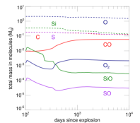
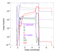
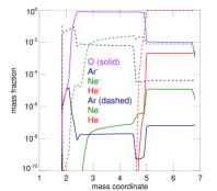
Figure 14: Evolution of the mass in common molecular species (left), mass fraction versus mass coordinate in common molecular species (middle), and mass fraction versus mass coordinate in weathering agents (right), each for the entire ejecta.

The left panel in Figure 14 shows the mass of CO, SiO, SO, and O₂ as a function of time in each of the density zones, as well as the mass of atomic C, O, Si, and S. In contrast to the dust mass, the mass in molecules is relatively constant over the entire $100$–$10^{4}$ day period. At the end of the simulation, the total mass in CO, SiO, SO, and O₂ is ($0.059$, $2.9\times 10^{-4}$, $3.1\times 10^{-5}$, $2.2\times 10^{-3})M_{\odot}$. Dissociation by Compton electrons and charge transfer reactions with noble gas ions, as well as depletion onto grains, keep the gas from turning fully molecular.

The middle panel in Figure 14 shows the mass fraction of these species as a function of mass coordinate in each density zone. Virtually no molecules form in the bubbles due to the low density and high ionization fraction. Outside of the bubbles molecules mostly form at mass coordinates $2\,M_{\odot}<M<5\,M_{\odot}$, with more molecules forming in the shells than in the ambient ejecta. At $M>5\,M_{\odot}$ the high abundance of helium suppresses molecules in both the ambient ejecta and the shells.

In the right panel in Figure 14 we show the mass fraction of the weathering agents He⁺, Ne⁺, Ar⁺, and O as a function of mass coordinate. It can be seen that noble gas weathering is dominated by helium for $M>5\,M_{\odot}$, neon for $3\,M_{\odot}<M<5\,M_{\odot}$, and argon for $M<3\,M_{\odot}$. Since the mass fraction of Ne⁺ and Ar⁺ for $M<5\,M_{\odot}$ is $10^{4}$ times below that of He⁺ for $M>5\,M_{\odot}$, neon and argon weathering are relatively insignificant compared to helium weathering. The large diversity of grain species over the mass coordinates $2\,M_{\odot}<M<5\,M_{\odot}$ is in part due to the lack of noble gas weathering agents there. However, oxygen is very abundant in this region and its weathering suppresses carbon grain formation.

6.3 Dependance on shell density

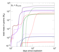
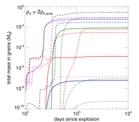
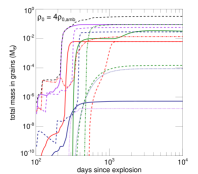
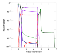
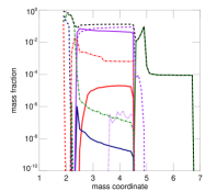
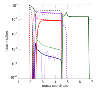
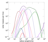
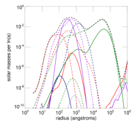
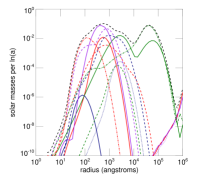
Figure 15: Grain properties in shells of different density. From left to right the shell mass density is 1, 2, and 4 times the ambient ejecta density. From top to bottom the grain properties shown are grain mass versus time, grain mass fraction versus mass coordinate, and (logarithmic) grain mass distribution. The grain species legend is the same as in Figure 13.

Recall that we varied the shell density between 1, 2, and 4 times the mass density in the ambient ejecta. The corresponding grain masses as a function of time, grain mass fractions as a function of the enclosed mass, and grain size distributions at the end of the simulation are shown in Figure 15. Grains form slightly earlier at higher shell densities and the total dust mass is larger. The dust mass created in the shells can be approximated with the power law:

$$M_{\rm dust,shell,1987A}=0.22\,M_{\odot}\times\left(\frac{\rho_{0}}{4\times 10^{-13}\,\textrm{g}\,\textrm{cm}^{-3}}\right)^{0.26},$$ (81)

where $\rho_{0}$ is the shell density at 100 days. The normalization factor in Equation (81) is of course specific to our model of SN 1987A. The grain species mass fractions at a given mass coordinate are not very sensitive to the mass density in the shell, except for those of alumina and carbon grains. In the case of alumina, its abundance in the region $2.5\,M_{\odot}<M<4.5\,M_{\odot}$ sharply increases with density. Similarly, the abundance of carbon grains increases in the helium shell $M>5\,M_{\odot}$.

7 Discussion

7.1 Comparison with previous work in MNT

Recall that there are three frameworks for modeling dust formation in supernovae, in the increasing order of computational complexity: classical nucleation theory (CNT), kinetic nucleation theory (KNT), and molecular nucleation theory (MNT). Our work is an extension of MNT, which was developed in Cherchneff & Lilly (2008), Cherchneff & Dwek (2009, 2010), Sarangi & Cherchneff (2013, 2015), and Biscaro & Cherchneff (2014, 2016).

Our model is similar to that of Sarangi & Cherchneff (2015) (hereafter SC15). These authors used MNT to compute the grain mass versus time and grain size distribution for 8 grain species (forsterite, alumina, carbon, magnesium, silicon carbide, silicon, iron, and iron sulfide). They considered four explosion scenarios involving two progenitor masses, $15\,M_{\odot}$ and $19\,M_{\odot}$, and ran the simulations from 100 to 2000 days after the explosion. For the $15\,M_{\odot}$ progenitor they considered a case with normal ⁵⁶Ni production and a case with a ⁵⁶Ni mass of only $0.01\,M_{\odot}$. For the $19\,M_{\odot}$ progenitor they considered smooth as well as clumpy ejecta. In all cases they divided the ejecta into 6 or 7 annular shells, each of which was characterized by a density, temperature, elemental composition, and number and size of clumps.

Before comparing our simulation results to SC15, we should note some model differences other than physical process prescriptions; we discuss those at the end of this subsection. The mass densities in their zones were approximately 1.6 times our shell density in their $15\,M_{\odot}$ progenitor models and 0.62 times our shell density in their $19\,M_{\odot}$ progenitor models. In the clumps in their $19\,M_{\odot}$ progenitor models the density varied from 8 to 162 times our shell density. Overall, their densities are higher than ours by as much as two orders of magnitude. The temperatures in SC15 are higher than ours initially, at $\sim 100$ days, but as they follow power-laws, they drop below our temperatures after few hundred days (recall that we explicitly model, but the power-laws ignore, the late heating by ⁵⁷Co and ultimately ⁴⁴Ti radioactivity that slows the early cooling trend). The elemental compositions in SC15 are averaged over coarse annual shells, while ours are taken from discrete mass coordinates each having a different composition as provided by the mesa calculation; therefore, we do not assume that the explosion hydrodynamics can drive microscopic mixing. Finally, we include six additional grain species: enstatite, magnetite, silicon dioxide, magnesium sulfide, magnesia, and iron oxide.

For concreteness, we focus comparison on SC15’s $19\,M_{\odot}$ model with clumpy ejecta that is the closest to our simulation other than for having much higher ejecta density. At 2000 days after the explosion, the dust mass in our model was $0.44\,M_{\odot}$ while it was $0.14\,M_{\odot}$ in theirs. Our higher mass can be attributed to grain growth by accretion; SC15 included only growth by coagulation. Our overall grain mass evolution for forsterite, alumina, iron sulfide, and silicon is similar to that in the SC15 model, although in each case these grain species form later in our simulations owing to lower densities. Carbon grains form much earlier in our simulations than in the SC15 model, while magnesium grains are completely absent in our simulation but are present in theirs. The lack of magnesium grains in our simulation is due to quick elemental magnesium depletion into magnesia grains, a species not included in SC15. The peak radii of the grain mass distributions agree to within a factor of a few for forsterite, carbon, alumina, iron, and iron sulfide. Our silicon mass distribution peaks at significantly larger radii than in the SC15 model.

We now return to the physical process improvements over SC15. We include the effects of evaporation (sublimation) on grain growth and of finite grain size on the evaporation rate. We include the weathering of grains by noble gas ions and oxygen atoms (the latter in the case of carbon grains), whereas SC15 included only the corresponding processes for molecules. We compute the grain temperature to which the evaporation rate is sensitive separately from the gas temperature. In fact, it seems that most previous investigations simply set the dust temperature equal to the gas temperature (SC15 did not need the grain temperature as they did not treat evaporation). We compute the grain charge and its effects on the coagulation rate. We treat grain growth by accretion and coagulation, whereas SC15 treated only the latter process. We extend our simulation to $10^{4}$ days and include the effects of radioactive decay of ^56,57Co, ⁴⁴Ti, and ²²Na on the ejecta temperature evolution and chemistry and on grain temperature and charge; SC15 simulated to 2,000 days and only treated ⁵⁶Co decay.

7.2 Observations

As dust begins to form, it reprocesses the optical and UV into the IR. The thermal emission from dust is initially in the near-IR (for $T_{\rm dust}>500K$) but gradually shifts to the mid-IR (for $100\,\textrm{K}<T_{\rm dust}<500\,\textrm{K}$) and ultimately the far-IR (for $T_{\rm dust}<100K$). Much of the thermal radiation emitted by grains cannot be observed from the earth’s surface due to atmospheric absorption. At the time that SN 1987A was observed, there would not be infrared space telescopes for another 8 years. However, measurements of the infrared SED were made from the Kuiper Airborne Observatory (KAO) at 60, 250, 415, 615, and 775 days after the explosion (Wooden et al., 1993). Note the 200 day gap in the observations between 415 and 615 days. This is the period when most of the dust mass seems to have formed, as the percentage of the bolometric luminosity contributed by the IR jumps from 2% at 415 days to 45% at 615 days and then to 83% at 775 days. The much later mid-IR observations with the Spitzer Space Telescope (after 5,800 days), the far-IR observations with the Herschel Space Observatory (after 8,000 days), and sub-mm observations with ALMA (after 9,000 days) are now providing a much more complete picture of dust properties in the remnant.

Attempts have been made to use the observations from KAO, Spitzer, Herschel, and ALMA (and optical/UV observations from telescopes such as the Hubble Space Telescope) to determine the time evolution of grain properties in the ejecta of SN 1987A. This is done by fitting a dust reprocessing model to the SED. The ejecta is assumed to be divided into an inner heavy element core where grains form in high density clumps, a helium shell, and a hydrogen envelope. The grain mass, composition, size distribution, spatial distribution within clumps, and as well as the clump spatial distribution are varied until the resulting SED matches the observations. We discuss the three major attempts to do this in SN 1987A: Wesson et al. (2015), Bevan & Barlow (2016), and Dwek & Arendt (2015).

Wesson et al. (2015) used three dimensional radiative transfer simulations with mocassin (Ercolano et al., 2005) to calculate the SED of SN 1987A over the wavelength range $0.3\,\textrm{$\mu$m}<\lambda<100\,\textrm{$\mu$m}$ at 615, 775, 1153, 1300, 8515, and 9200 days after the explosion. They found that in order to match the observed SEDs, the grain mass should increase from $0.001\,M_{\odot}$ at 615 days to $0.8\,M_{\odot}$ at 9200 days and that the grain size distribution has power-law slope $dN/da\propto a^{-3.5}$ with grain sizes between $0.005\,\textrm{$\mu$m}$ and $0.25\,\textrm{$\mu$m}$ in the period between 615 and 1300 days and between $3.005\,\textrm{$\mu$m}$ and $3.25\,\textrm{$\mu$m}$ in the period between 8515 and 9200 days. The grain mass increases from $0.02\,M_{\odot}$ at 1300 days to $0.6\,M_{\odot}$ at 8515 days. This means that 72.5% of the final dust mass formed between these two times and that 25% of the dust mass formed between 8515 and 9090 days (so that 97.5% of the dust mass formed after 1300 days).

Bevan & Barlow (2016) performed three dimensional Monte Carlo radiative transfer to model the emission line blueshifting in the presence of dust. Their results fill in some of the gaps between days 1300 and 8515 in Wesson et al. (2015). The results of Wesson et al. (2015) and Bevan & Barlow (2016) can be combined to arrive at the conclusion—one that is controversial in view of the remaining of the three observational attempts and the theoretical predictions of SC15—that dust mass increases as a power law in time: $M_{\rm dust,tot,1987A}\propto t^{2.5}$. These results, which assume spherically-symmetric ejecta, are questioned by Larsson et al. (2016), who used spatially resolved spectra at optical and near IR wavelengths to determine the 3D distribution of H, He, O, Mg, Si, Ca, and Fe at $10^{4}$ days. The distribution of these elements was sufficiently anisotropic to explain on its own the spectral line distortion that Bevan & Barlow (2016) attribute to dust.

Dwek & Arendt (2015) used observations at 615, 775, 1144, 8815, and 9090 days and modeled the dust as amorphous carbon and enstatite. At 615, 775, and 1144 days, the clumps are optically thick to the radiation emitted by the grains and the ejecta already contains $0.4\,M_{\odot}$ of enstatite and $0.047M_{\odot}$ of carbon. By 8815 days the clumps become optically thin and the carbon and enstatite have coagulated to make composite grains that are essentially an enstatite matrix with carbon inclusions (18% of the volume of the grains is occupied by the carbon inclusions). The total dust mass is $0.42\,M_{\odot}$ at 8815 days and $0.45\,M_{\odot}$ at 9090 days.

While the estimates of Bevan & Barlow (2016) and Wesson et al. (2015) agree, they differ drastically with those of Dwek & Arendt (2015). The most important difference is that dust mass continuously increases for all times after 615 days in Bevan & Barlow (2016) and Wesson et al. (2015) while almost all of the dust has already formed by 615 days in Dwek & Arendt (2015). It is important to note that the discrepancy in inferred dust mass between the groups is highest at 615 days when the estimates differ by a factor of 447 and decreases with time, coming into near agreement at 9090 days. Another discrepancy is in the inferred composition: Wesson et al. (2015) find that 15% of the dust mass is in silicates and 85% is in carbon while Dwek & Arendt (2015) find that 89.5% of the dust mass is in enstatite (a silicate) and 10.5% in carbon.

The disagreement in the first 1000 days may be due to the very different approaches to radiative transfer by Wesson et al. (2015) and Dwek & Arendt (2015). Wesson et al. (2015) used a fully 3D radiative transfer calculation to model the SED while Dwek & Arendt (2015) used a simple formula for the probability that a photon will escape from a dusty sphere. The two techniques give dramatically different values for what the flux at $100\,\textrm{$\mu$m}$ should be for a given amount of dust mass (the observed flux at 626 days at $100\,\textrm{$\mu$m}$ is $0.6\,\textrm{Jy}$). According to Wesson et al. (2015), the dust mass at 615 days cannot exceed $0.01\,M_{\odot}$ since otherwise the flux at $100\,\textrm{$\mu$m}$ would exceed $0.6\,\textrm{Jy}$. On the other hand, according to Dwek & Arendt (2015) the observed flux at $100\,\textrm{$\mu$m}$ is exactly what it should be if there were $0.447\,M_{\odot}$ of dust at 615 days. At late times (9090 days) the ejecta is optically thin to dust thermal emission and so the dust mass is (relatively) straightforward to determine from far-IR Herschel and sub-mm ALMA observations.

At the time of writing the discrepancy in dust mass inferred at early times by different groups is unresolved, and it seems that more realistic radiative transfer modeling is required to settle the matter of the early dust mass in SN 1987A. Most authors assume that the grains are a mixture of carbon, iron, and enstatite (or other silicates), but our calculations suggest that at 615 days most of the dust mass is in magnesia, forsterite, silicon, and iron sulfide. Most groups also assume that the size distribution scales as $dN/da\propto a^{-3.5}$, but we find that each grain species has its own size distribution and that the total grain size is steeper $dN/da\propto a^{-4.39}$. Most groups assume that all grains are in dense clumps (what we would call dense shells), but we find that at 615 days the unclumped ambient ejecta contains 27% of the dust mass. Radiative transfer should further take into account the very low density cavities of the fossil nickel bubbles and consider the possibility that dust rich clumps occupy much less volume than currently assumed.

We finally note that magnesia has not been detected in SN 1987A, nor has it been detected in the observations of other supernovae. We speculate that the high abundance of MgO in our simulations is an artifact of not allowing MgO monomers and clusters to merge with other grain species. As is evident in Figure 11, where MgO forms in significant amounts, forsterite is also plentiful. It could be that in reality, the MgO monomers and clusters that form are aways absorbed into forsterite grains and do not exist as MgO monomers and grains. If this hypothesis is true, it explains the absence of detection of MgO in existing observations and also diminishes the promise of detection of MgO in future observations.

7.3 Future directions

Many aspects of our model of dust formation in supernova could be improved and made more realistic. We briefly mention a few. The degradation of the energy released by decaying radioactive nuclei, starting with $\gamma$-rays, should be followed with a Monte Carlo simulation (see, e.g., Hungerford, 2004; Jerkstrand et al., 2011). Such a simulation would provide the local, time-dependent gas temperature and ionization fraction in the ejecta as a function of time and an accurate model for the UV radiation field SED. These simulations need to take into account the asymmetric distribution of radioactive material, such as from the three-dimensional, neutrino-driven core-collapse simulation of Wongwathanarat et al. (2017) modeling Cas A. In post-processing they computed the local ⁴⁴Ti and ⁵⁶Ni yield in the ejecta finding that the ⁴⁴Ti distribution was very asymmetrical, with the bulk of isotope ejected into the hemisphere opposite to the neutron star kick.

Grain temperature can fluctuate stochastically, which, owing to the exponential dependence of the evaporation rate on temperature, has been found to influence grain growth in AGB stellar outflows (Kochanek, 2014). Compton-electron-induced destruction reactions should be included for all atoms, molecules, and dust grains. Ionization and molecular dissociation by UV photons should also be included. The destructive reactions with He⁺, Ne⁺, and Ar⁺ should be included for all neutral molecules. Grain-species-specific absorption coefficients and photoelectric yields should be used in the place of our carbon grain-based model.

Perhaps more consequentially, we do not expect that the dust grains have spherical shapes (Fallest et al., 2011). They could have porous and even fractal-like structures. The shape complexity could imply some very different thermodynamic, chemical, and optical behavior (e.g., Keith & Lazzati, 2011). While a fully realistic treatment of grain shapes will remain beyond reach, the salient effects of shape complexity should be assessed and incorporated in dust synthesis models. We also note that many of the chemical reaction rates used in this and preceding investigations of astrophysical dust synthesis are unverified extrapolations of sparsely-cataloged laboratory measurements. With the rapid development of ab initio electronic structure methods, it is now becoming possible to complement laboratory data with theoretical calculations. For example, Mauney et al. (2015) recently reported density function theory (DFT) based calculations of the work of small carbon cluster formation and the nucleation rate in a saturated, hydrogen-poor carbon gas. The new quantum electrodynamical time-dependent DFT (Flick et al., 2015) should enable direct computation of collisional cross sections involving photon emission, such as for radiative association in the formation small grain-precursor atomic clusters.

The dust produced in our calculation must pass a reverse shock before joining the ISM. Sputtering in the reverse shock destroys small grains and reduces the large ones. Therefore, dust survival hinges on the grain size distribution (e.g., Bianchi et al., 2009). This effect can be studied in Cassiopeia A where the reverse shock has already crossed a fraction of the dust-forming ejecta (Nozawa et al., 2010). The characteristic minimum size for a grain to survive the reverse shock may be $\sim 0.1\,\mu\text{m}$ (Silvia et al., 2010, 2012). Our calculation produces an abundance of such large grains. Since the reverse shock diminishes in clumps, our hypothesized ejecta clumpiness, in the form of thin shells compressed by overpressured nickel bubbles, serves to protect the grains in clumps from the reverse shock (Biscaro & Cherchneff, 2016).

8 Conclusions

We simulated the formation molecules and dust grains in the ejecta of SN 1987A using an improved molecular nucleation theory model. The model assumes that ⁵⁶Ni-rich clumps are injected into the helium core where they expand and sweep up dense shells of ambient ejecta. We compute the abundance of molecules as a function of time using a nonequilibrium chemical reaction network including the effects of radioactive decay of ⁵⁶Ni, ⁵⁷Ni, ⁴⁴Ti, and ²²Na. Grain formation starts with the formation of condensation nuclei which are treated as molecular species in the chemical network. The nuclei grow into grains via accretion and coagulation. Grain charge and van der Waals interaction are explicitly calculated to correct the coagulation rate. Grain destruction by oxygen and noble gas weathering is included, as is evaporation. To get the evaporation rate, we explicitly compute the grain temperature as a function of radius and account for the finite grain size.

The model produces a total dust mass of $0.51\,M_{\odot}$, which is 16% of the mass of refractory elements. Grain formation is rapid between 200 and 600 days and slower thereafter. At 615 days, our computed total grain mass agrees with the observational estimate of Dwek & Arendt (2015) but not with those of Wesson et al. (2015) and Bevan & Barlow (2016). We find that the dust mass produced in the dense shells scales as the 0.26 power of the mass density in the shells. The final computed dust mass is close to, and bracketed by, the observationally inferred dust masses in SN 1987A. The mass distribution $dM_{\rm dust}/d\ln a$ peaks at the grain radius $a=680\,\textrm{\AA}$. Beyond this peak, the size distribution scales as $dN/d\ln a\propto a^{-3.4}$, and the overall distribution is skewed toward larger grains. The most common grain species by mass are magnesia (32%), silicon (29%), forsterite (18%), iron sulfide (7.8%), and carbon (6.1%). The dense shells produced more dust mass and a greater variety of grain species than the ambient ejecta whereas grain formation in the nickel bubbles was negligible.

Finally, we note the numerical complexity of dust synthesis calculations. To validate calculations such as ours, it is necessary to run different codes on the same or similar models and compare the results. We are encouraged that dust composition and the timing of dust growth closely resemble those in Sarangi & Cherchneff (2015).

9 Appendix

In this Appendix we provide our isotope to element conversion table (Table 12) and tables of chemical reactions included in our model as well as some additional reactions (the remaining tables). The additional reactions not included in our chemical network are those involving nitrogen, charged molecules with three or more atoms, and the molecules CS, CSO, C₂O, CO₂, SO₂, S₂, SiS, and their charged counterparts. We provide these reactions for the convenience of the reader who wishes to use a more comprehensive reaction network.

The reaction source references indicated with acronyms are the University of Manchester Institute of Science and Technology (UMIST) Database for Astrochemistry
(U12; McElroy et al. 2013; http://udfa.ajmarkwick.net/) and National Institute of Standards and Technology (NIST) Chemical Kinetics Database
(http://kinetics.nist.gov/kinetics/KineticsSearchForm.jsp).

In the reaction tables the last column is the reference that describes how we obtained the rate coefficient. If a paper or database is cited in the column, we either use the rate coefficient cited in the source or estimate it from information in the source. If a reaction has a reference with the statement “$=$ X", then its rate coefficient could not be found in the literature and is duplicated from a similar reaction X. Reactions with reference “O" use the rate coefficient for $\mbox{C}_{n}+\mbox{O}\to\mbox{C}_{n-1}+\mbox{CO}$ from Lazzati & Heger (2016) while reactions with reference “He⁺" use the rate coefficient for $\mbox{C}_{n}+\mbox{He}^{+}\to\mbox{C}_{n-1}+\mbox{C}^{+}+\mbox{He}$, from the same reference. Reactions with reference “Est" used the formulas in Section 3.2. All three-body reactions use the same rate coefficient derived in that section, even if they have rate coefficients given in the literature, because the published rates are only valid at high temperatures.

Element	Isotopes
H	1H, 2H
He	3He, 4He, 8B
Li	6Li, 7Li, 7Be
Be	9Be, 10Be
B	10B, 11B
C	12C, 13C, 13N
N	14N, 15N, 15O
O	16O, 17O, 18O, 16N, 17F, 18F
F	19F, 19O, 19Ne
Ne	20Ne, 21Ne, 22Ne, 20F, 21Na, 22Na
Na	23Na, 23Ne, 23Mg
Mg	24Mg, 25Mg, 26Mg, 24Na, 25Al
Al	26Al, 27Al, 27Mg, 27Si
Si	28Si, 29Si, 30Si, 28Al, 32Si, 30P
P	31P, 31Si, 31S
S	32S, 33S, 34S, 36S, 33Si, 32P, 33P, 34P
Cl	35Cl, 36Cl, 37Cl, 35S, 37S, 35Ar, 37Ar
Ar	36Ar, 38Ar, 39Ar, 40Ar, 38Cl
K	39K, 40K, 41K, 41Ar, 39Ca
Ca	40Ca, 41Ca, 42Ca, 43Ca, 44Ca, 46Ca, 48Ca, 42K, 43K,
	44K,43Sc,44Sc, 43Ti
Sc	45Sc, 45Ca, 45Ti
Ti	44Ti, 46Ti, 47Ti, 48Ti, 49Ti, 50Ti, 47Ca, 49Ca, 46Sc,
	47Sc, 48Sc,49Sc, 50Sc, 47V, 48V, 49V, 47Cr, 48Cr, 49Cr
V	50V, 51V, 51Sc, 51Ti, 51Cr, 51Mn, 51Fe
Cr	50Cr, 52Cr, 53Cr, 54Cr, 52Ti, 53Ti, 54Ti, 52V, 53V, 54V,
	54Mn,52Fe
Mn	55V, 55Cr, 55Mn, 53Fe, 55Fe, 55Co, 55Ni
Fe	54Fe, 56Fe, 57Fe, 58Fe, 56V, 56Cr, 57Cr, 58Cr, 56Mn,
	57Mn, 58Mn, 60Fe, 56Co, 57Co, 58Co, 56Ni, 57Ni
Co	59Mn, 59Fe, 59Co
Ni	61Fe, 62Fe, 63Fe, 64Fe, 60Co, 61Co, 62Co, 63Co, 64Co,
	58Ni,59Ni, 60Ni, 61Ni, 62Ni, 63Ni, 64Ni, 59Cu, 60Cu,
	61Cu, 62Cu, 64Cu, 59Zn, 60Zn, 61Zn, 62Zn
Cu	65Fe, 65Co, 65Ni, 63Cu, 65Cu, 63Zn, 65Zn
Zn	66Fe, 66Co, 67Co, 66Ni, 67Ni, 68Ni, 66Cu, 64Zn, 66Zn

Table 12: Isotope to element conversion.

Code	Reaction	$A\ (\text{cgs})$	$\nu$	$T_{\rm A}\ (\text{K})$	Ref.
A1	$\rm C+O\to CO+\gamma$	$4.69\times 10^{-19}$	$1.52$	$-50.5$	U12
A2	$\rm C+C\to C_{2}+\gamma$	$4.36\times 10^{-18}$	$0.35$	$161.3$	U12
A4	$\rm C^{+}+C_{3}\to C_{4}^{+}+\gamma$	$1\times 10^{-13}$	$-1$	$0$	U12
A11	$\rm C^{+}+C\to C_{2}^{+}+\gamma$	$4.01\times 10^{-18}$	$0.17$	$101.5$	U12
A12	$\rm C^{+}+N\to CN^{+}+\gamma$	$1.08\times 10^{-18}$	$0.07$	$57.5$	U12
A13	$\rm C^{+}+O\to CO^{+}+\gamma$	$3.14\times 10^{-18}$	$-0.15$	$68$	U12
A14	$\rm C^{+}+S\to CS^{+}+\gamma$	$3.07\times 10^{-19}$	$0.15$	$0$	U12
A15	$\rm C+C_{2}\to C_{3}+\gamma$	$3\times 10^{-16}$	$-1$	$0$	U12
A16	$\rm C+C_{3}\to C_{4}+\gamma$	$4\times 10^{-14}$	$-1$	$0$	U12
A17	$\rm C+N\to CN+\gamma$	$5.72\times 10^{-19}$	$0.37$	$51$	U12
A18	$\rm C+O^{+}\to CO^{+}+\gamma$	$5\times 10^{-10}$	$-3.7$	$800$	U12
A19	$\rm C+S^{+}\to CS^{+}+\gamma$	$2.01\times 10^{-18}$	$0.07$	$301$	U12
A20	$\rm C+S\to CS+\gamma$	$4.36\times 10^{-19}$	$0.22$	$0$	U12
A21	$\rm N^{+}+N\to N_{2}^{+}+\gamma$	$3.71\times 10^{-18}$	$0.24$	$26.1$	U12
A22	$\rm O+O\to O_{2}+\gamma$	$4.9\times 10^{-20}$	$1.58$	$0$	U12
A23	$\rm O+SO\to SO_{2}+\gamma$	$3.2\times 10^{-16}$	$-1.5$	$0$	U12
A24	$\rm O+Si^{+}\to SiO^{+}+\gamma$	$9.22\times 10^{-19}$	$-0.08$	$-21.2$	U12
A25	$\rm O+Si\to SiO+\gamma$	$5.52\times 10^{-18}$	$0.31$	$0$	U12
A26	$\rm O+S\to SO+\gamma$	$1.114\times 10^{-19}$	$0.2761$	$1297.9$	AM05
A27	$\rm S+S\to S_{2}+\gamma$	$1.374\times 10^{-19}$	$0.3339$	$-78.801$	AM05
A28	$\rm Si+S\to SiS+\gamma$	$1.047\times 10^{-16}$	$0.301$	$66.093$	AM05

Table 13: Reaction Set A (Radiative Association Reactions). Note that AM05 refers to Andreazza & Marinho (2005).

Code	Reaction	$A\ (\text{cgs})$	$\nu$	$T_{\rm A}\ (\text{K})$	Ref.
B1	$\rm C+C+M\to C_{2}+M$	$4.25\times 10^{-34}$	1	0	Derived in Section 3.2
B2	$\rm C+N+M\to CN+M$	$4.25\times 10^{-34}$	1	0	Derived in Section 3.2
B3	$\rm C+O+M\to CO+M$	$4.25\times 10^{-34}$	1	0	Derived in Section 3.2
B4	$\rm C^{+}+O+M\to CO^{+}+M$	$4.25\times 10^{-34}$	1	0	Derived in Section 3.2
B5	$\rm C+O^{+}+M\to CO^{+}+M$	$4.25\times 10^{-34}$	1	0	Derived in Section 3.2
B6	$\rm C+CO+M\to C_{2}O+M$	$4.25\times 10^{-34}$	1	0	Derived in Section 3.2
B7	$\rm O+O+M\to O_{2}+M$	$4.25\times 10^{-34}$	1	0	Derived in Section 3.2
B8	$\rm O+NO+M\to NO_{2}+M$	$4.25\times 10^{-34}$	1	0	Derived in Section 3.2
B9	$\rm O+SO+M\to SO_{2}+M$	$4.25\times 10^{-34}$	1	0	Derived in Section 3.2
B10	$\rm O+S+M\to SO+M$	$4.25\times 10^{-34}$	1	0	Derived in Section 3.2
B11	$\rm O+N+M\to NO+M$	$4.25\times 10^{-34}$	1	0	Derived in Section 3.2
B12	$\rm O+CO+M\to CO_{2}+M$	$4.25\times 10^{-34}$	1	0	Derived in Section 3.2
B13	$\rm O+Si+M\to SiO+M$	$4.25\times 10^{-34}$	1	0	Derived in Section 3.2
B14	$\rm C+C_{2}+M\to C_{3}+M$	$4.25\times 10^{-34}$	1	0	Derived in Section 3.2
B15	$\rm C+S+M\to CS+M$	$4.25\times 10^{-34}$	1	0	Derived in Section 3.2
B16	$\rm Si+N+M\to SiN+M$	$4.25\times 10^{-34}$	1	$0$	Derived in Section 3.2
B17	$\rm Si+S+M\to SiS+M$	$4.25\times 10^{-34}$	1	0	Derived in Section 3.2
B18	$\rm S+S+M\to S_{2}+M$	$4.25\times 10^{-34}$	1	0	Derived in Section 3.2
B19	$\rm N+N+M\to N_{2}+M$	$4.25\times 10^{-34}$	1	0	Derived in Section 3.2

Table 14: Reaction Set B (Three-Body Reactions).

Code	Reaction	$A\ (\text{cgs})$	$\nu$	$T_{\rm A}\ (\text{K})$	Ref.
C1	$\rm CO+M\to O+C+M$	$2.86\times 10^{-3}$	$-3.52$	$112700$	U12
C2	$\rm C_{2}+M\to C+C+M$	$2.49\times 10^{-8}$	$0$	$71561.6$	NIST
C3	$\rm O_{2}+M\to O+O+M$	$1.01\times 10^{-8}$	$-1$	$59414.2$	NIST
C4	$\rm SO+M\to S+O+M$	$6.61\times 10^{-10}$	$0$	$53881.7$	NIST
C5	$\rm SiO+M\to Si+O+M$	$2.86\times 10^{-3}$	$-3.52$	$112700$	$=$ C1
C6	$\rm NO+M\to N+O+M$	$4\times 10^{-9}$	$0$	$74568.4$	NIST
C7	$\rm CO_{2}+M\to CO+O+M$	$4.17\times 10^{-11}$	$0$	$43778.9$	NIST
C8	$\rm CS+M\to C+S+M$	$2.86\times 10^{-3}$	$-3.52$	$112700$	$=$ C1
C9	$\rm CN+M\to C+N+M$	$3.32\times 10^{-10}$	$0$	$75049.5$	NIST
C10	$\rm SiS+M\to Si+S+M$	$2.86\times 10^{-3}$	$-3.52$	$112700$	$=$ C1
C11	$\rm SiN+M\to Si+N+M$	$3.32\times 10^{-10}$	$0$	$75049.5$	$=$ C9
C12	$\rm S_{2}+M\to S+S+M$	$7.95\times 10^{-11}$	$0$	$38727.5$	NIST
C13	$\rm N_{2}+M\to N+N+M$	$2.52\times 10^{-7}$	$-1.6$	$57008.8$	NIST

Table 15: Reaction Set C (Thermal Fragmentation Reactions).

Code	Reaction	$A\ (\text{cgs})$	$\nu$	$T_{\rm A}\ (\text{K})$	Ref.
D1	$\rm C+CO\to C_{2}+O$	$2.94\times 10^{-11}$	$0.5$	$58025$	U12
D2	$\rm O+C_{2}\to CO+C$	$2\times 10^{-10}$	$-0.12$	$0$	U12
D3	$\rm C_{2}+O_{2}\to CO+CO$	$1.5\times 10^{-11}$	$0$	$4300$	U12
D5	$\rm C_{2}+S\to CS+C$	$1\times 10^{-10}$	$0$	$0$	U12
D7	$\rm C+C_{2}O\to C_{2}+CO$	$2\times 10^{-10}$	$0$	$0$	U12
D10	$\rm C+C_{4}\to C_{2}+C_{3}$	$9\times 10^{-11}$	$0$	$0$	U12
D19	$\rm C+CN\to C_{2}+N$	$4.98\times 10^{-10}$	$0$	$18116$	U12
D20	$\rm C+CS\to S+C_{2}$	$1.44\times 10^{-11}$	$0.5$	$20435$	U12
D21	$\rm C+N_{2}\to CN+N$	$8.69\times 10^{-11}$	$0$	$22600$	U12
D23	$\rm C+NO\to CN+O$	$6\times 10^{-11}$	$-0.16$	$0$	U12
D24	$\rm C+NO\to CO+N$	$9\times 10^{-11}$	$-0.16$	$0$	U12
D25	$\rm C+NS\to CS+N$	$1.73\times 10^{-11}$	$0.5$	$4000$	U12
D26	$\rm C+NS\to S+CN$	$1.5\times 10^{-10}$	$-0.16$	$0$	U12
D27	$\rm C+O_{2}\to CO+O$	$5.56\times 10^{-11}$	$0.41$	$-26.9$	U12
D28	$\rm C+CNO\to CO+CN$	$1\times 10^{-10}$	$0$	$0$	U12
D30	$\rm C+S_{2}\to CS+S$	$7\times 10^{-11}$	$0$	$0$	U12
D31	$\rm C+SO_{2}\to CO+SO$	$7\times 10^{-11}$	$0$	$0$	U12
D32	$\rm C+SO\to CS+O$	$3.5\times 10^{-11}$	$0$	$0$	U12
D33	$\rm C+SO\to S+CO$	$3.5\times 10^{-11}$	$0$	$0$	U12
D34	$\rm CN+CN\to N_{2}+C_{2}$	$2.66\times 10^{-9}$	$0$	$21638$	U12
D35	$\rm CN+NO_{2}\to NO+CNO$	$7.02\times 10^{-11}$	$-0.27$	$8.3$	U12
D36	$\rm CN+NO\to N_{2}+CO$	$1.6\times 10^{-13}$	$0$	$0$	U12
D37	$\rm CN+NO\to CNO+N$	$1.62\times 10^{-10}$	$0$	$21205$	U12
D38	$\rm CN+O_{2}\to NO+CO$	$5.12\times 10^{-12}$	$-0.49$	$-5.2$	U12
D39	$\rm CN+O_{2}\to CNO+O$	$2.02\times 10^{-11}$	$-0.19$	$-31.9$	U12
D40	$\rm CN+S\to NS+C$	$5.71\times 10^{-11}$	$0.5$	$32010$	U12
D41	$\rm CO+N_{2}O\to CO_{2}+N_{2}$	$1.62\times 10^{-13}$	$0$	$8780$	U12
D42	$\rm CO+NO_{2}\to CO_{2}+NO$	$1.48\times 10^{-10}$	$0$	$17000$	U12
D43	$\rm CO+O_{2}\to CO_{2}+O$	$5.99\times 10^{-12}$	$0$	$24075$	U12
D44	$\rm N_{2}+O_{2}\to N_{2}O+O$	$1\times 10^{-10}$	$0$	$55200$	U12
D46	$\rm N+C_{2}\to CN+C$	$5\times 10^{-11}$	$0$	$0$	U12
D48	$\rm N+C_{2}O\to CN+CO$	$5.5\times 10^{-10}$	$0$	$0$	U12
D49	$\rm N+C_{3}\to CN+C_{2}$	$1\times 10^{-13}$	$0$	$0$	U12
D51	$\rm N+C_{4}\to C_{3}+CN$	$1\times 10^{-10}$	$0$	$0$	U12

Table 16: Reaction Set D (Neutral-Neutral Reactions).

Code	Reaction	$A\ (\text{cgs})$	$\nu$	$T_{\rm A}\ (\text{K})$	Ref.
D61	$\rm N+CN\to N_{2}+C$	$1\times 10^{-10}$	$0.18$	$0$	U12
D62	$\rm N+CO_{2}\to NO+CO$	$3.2\times 10^{-13}$	$0$	$1710$	U12
D63	$\rm N+CS\to S+CN$	$3.8\times 10^{-11}$	$0.5$	$1160$	U12
D65	$\rm N+NO_{2}\to N_{2}+O+O$	$2.41\times 10^{-12}$	$0$	$0$	U12
D66	$\rm N+NO_{2}\to N_{2}O+O$	$3\times 10^{-12}$	$0$	$0$	U12
D67	$\rm N+NO_{2}\to NO+NO$	$1\times 10^{-12}$	$0$	$0$	U12
D68	$\rm N+NO_{2}\to O_{2}+N_{2}$	$1\times 10^{-12}$	$0$	$0$	U12
D69	$\rm N+NO\to N_{2}+O$	$3.38\times 10^{-11}$	$-0.17$	$-2.8$	U12
D70	$\rm N+NS\to S+N_{2}$	$3\times 10^{-11}$	$-0.6$	$0$	U12
D71	$\rm N+O_{2}\to NO+O$	$2.26\times 10^{-12}$	$0.86$	$3134$	U12
D72	$\rm N+S_{2}\to NS+S$	$1.73\times 10^{-11}$	$0.5$	$4000$	U12
D73	$\rm N+SO\to NS+O$	$4.68\times 10^{-11}$	$0.5$	$8254$	U12
D74	$\rm N+SO\to S+NO$	$1.73\times 10^{-11}$	$0.5$	$750$	U12
D75	$\rm N+SiC\to Si+CN$	$5\times 10^{-11}$	$0$	$0$	U12
D76	$\rm N+SiC\to SiN+C$	$5\times 10^{-11}$	$0$	$0$	U12
D77	$\rm NO+N_{2}O\to NO_{2}+N_{2}$	$2.92\times 10^{-13}$	$2.23$	$23292$	U12
D78	$\rm NO+NO\to N_{2}O+O$	$7.22\times 10^{-12}$	$0$	$33155$	U12
D79	$\rm NO+NO\to O_{2}+N_{2}$	$2.51\times 10^{-11}$	$0$	$30653$	U12
D80	$\rm NO+O_{2}\to NO_{2}+O$	$2.8\times 10^{-12}$	$0$	$23400$	U12
D81	$\rm NO+CNO\to N_{2}+CO_{2}$	$4.55\times 10^{-11}$	$-1.33$	$242$	U12
D82	$\rm NO+CNO\to N_{2}O+CO$	$3.47\times 10^{-11}$	$-1.33$	$242$	U12
D83	$\rm NO+S\to NS+O$	$2.94\times 10^{-11}$	$0.5$	$17465$	U12
D84	$\rm NO+S\to SO+N$	$1.75\times 10^{-10}$	$0$	$20200$	U12
D85	$\rm O_{2}+CNO\to CO_{2}+NO$	$1.32\times 10^{-12}$	$0$	$0$	U12
D86	$\rm O_{2}+CNO\to NO_{2}+CO$	$8.1\times 10^{-11}$	$0$	$773$	U12
D87	$\rm O_{2}+S\to SO+O$	$1.76\times 10^{-12}$	$0.81$	$-30.8$	U12
D88	$\rm O_{2}+SO\to SO_{2}+O$	$1.1\times 10^{-14}$	$1.89$	$1538$	U12
D92	$\rm O+C_{2}O\to CO+CO$	$8.59\times 10^{-11}$	$0$	$0$	U12
D94	$\rm O+C_{3}\to CO+C_{2}$	$5\times 10^{-12}$	$0$	$900$	U12
D97	$\rm O+C_{4}\to C_{3}+CO$	$1\times 10^{-10}$	$0$	$0$	U12
D107	$\rm O+CN\to CO+N$	$2.54\times 10^{-11}$	$0$	$0$	U12
D108	$\rm O+CN\to NO+C$	$5.37\times 10^{-11}$	$0$	$13800$	U12
D109	$\rm O+CNO\to CO+NO$	$1\times 10^{-10}$	$0$	$0$	U12
D110	$\rm O+CO_{2}\to O_{2}+CO$	$2.46\times 10^{-11}$	$0$	$26567$	U12
D111	$\rm O+CS\to S+CO$	$2.48\times 10^{-10}$	$-0.65$	$783$	U12
D112	$\rm O+CS\to SO+C$	$4.68\times 10^{-11}$	$0.5$	$28940$	U12
D113	$\rm O+N_{2}\to NO+N$	$2.51\times 10^{-10}$	$0$	$38602$	U12
D114	$\rm O+N_{2}O\to NO+NO$	$1.15\times 10^{-10}$	$0$	$13400$	U12
D115	$\rm O+N_{2}O\to O_{2}+N_{2}$	$1.66\times 10^{-10}$	$0$	$14100$	U12
D116	$\rm O+NO_{2}\to O_{2}+NO$	$9.82\times 10^{-12}$	$-0.21$	$5.2$	U12
D117	$\rm O+NO\to O_{2}+N$	$1.18\times 10^{-11}$	$0$	$20413$	U12
D118	$\rm O+NS\to S+NO$	$1\times 10^{-10}$	$0$	$0$	U12
D119	$\rm O+NS\to SO+N$	$1\times 10^{-11}$	$0$	$0$	U12
D121	$\rm O+CNO\to O_{2}+CN$	$4.02\times 10^{-10}$	$-1.43$	$3501$	U12
D124	$\rm O+S_{2}\to SO+S$	$1.7\times 10^{-11}$	$0$	$0$	U12
D125	$\rm O+SO_{2}\to SO+O_{2}$	$9.01\times 10^{-12}$	$0$	$9837$	U12
D126	$\rm O+SO\to S+O_{2}$	$6.6\times 10^{-13}$	$0$	$2760$	U12
D130	$\rm O+SiC\to Si+CO$	$5\times 10^{-11}$	$0$	$0$	U12
D131	$\rm O+SiC\to SiO+C$	$5\times 10^{-11}$	$0$	$0$	U12
D132	$\rm O+SiN\to NO+Si$	$5\times 10^{-11}$	$0$	$0$	U12
D133	$\rm O+SiN\to SiO+N$	$5.75\times 10^{-11}$	$0.1$	$200$	U12
D135	$\rm S+C_{2}O\to CO+CS$	$1\times 10^{-10}$	$0$	$0$	U12
D136	$\rm S+SO_{2}\to SO+SO$	$9.76\times 10^{-12}$	$0$	$4545$	U12
D137	$\rm S+SO\to S_{2}+O$	$1.73\times 10^{-11}$	$0.5$	$11500$	U12
D138	$\rm Si+CO_{2}\to SiO+CO$	$2.72\times 10^{-11}$	$0$	$282$	U12
D139	$\rm Si+CO\to SiO+C$	$1.3\times 10^{-9}$	$0$	$34513$	U12

Table 17: Reaction Set D (Neutral-Neutral Reactions, continued).

Code	Reaction	$A\ (\text{cgs})$	$\nu$	$T_{\rm A}\ (\text{K})$	Ref.
D140	$\rm Si+NO\to SiO+N$	$9\times 10^{-11}$	$-0.96$	$28$	U12
D141	$\rm Si+O_{2}\to SiO+O$	$1.72\times 10^{-10}$	$-0.53$	$17$	U12
D142	$\rm O+CO\to O_{2}+C$	$1\times 10^{-16}$	$0$	$0$	CD09
D143	$\rm O+SiO\to O_{2}+Si$	$1\times 10^{-16}$	$0$	$0$	CD09
D144	$\rm C+SiO\to CO+Si$	$1\times 10^{-16}$	$0$	$0$	CD09
D145	$\rm Si+S_{2}\to SiS+S$	$7\times 10^{-11}$	$0$	$0$	$=$ D30
D146	$\rm C+CO_{2}\to CO+CO$	$1\times 10^{-15}$	$0$	$0$	NIST
D147	$\rm N+CO\to CN+O$	$3.84\times 10^{-9}$	$0$	$35961.2$	NIST
D148	$\rm N+CO\to NO+C$	$3.84\times 10^{-9}$	$0$	$35961.2$	$=$ D147
D149	$\rm S+CO\to SO+C$	$1\times 10^{-16}$	$0$	$0$	CD09
D150	$\rm S+CO\to CS+O$	$1\times 10^{-16}$	$0$	$0$	CD09
D151	$\rm S+CS\to S_{2}+C$	$1.73\times 10^{-11}$	$0.5$	$11500$	$=$ D137
D152	$\rm S+CN\to CS+N$	$2.54\times 10^{-11}$	$0$	$0$	$=$ D107
D153	$\rm S+SiS\to S_{2}+Si$	$5.75\times 10^{-11}$	$0.1$	$200$	$=$ D133
D154	$\rm N+SiO\to SiN+O$	$3.84\times 10^{-9}$	$0$	$35961.2$	$=$ D148
D155	$\rm N+SiO\to NO+Si$	$1\times 10^{-16}$	$0$	$0$	CD09
D156	$\rm N+SiS\to SiN+S$	$3.8\times 10^{-11}$	$0.5$	$1160$	$=$ D63
D157	$\rm O_{2}+N_{2}\to NO+NO$	$1\times 10^{-16}$	$0$	$0$	CD09
D158	$\rm CO+SiO\to CO_{2}+Si$	$1\times 10^{-16}$	$0$	$0$	CD09
D159	$\rm CO+NO\to CO_{2}+N$	$1\times 10^{-16}$	$0$	$0$	CD09

Table 18: Reaction Set D (Neutral-Neutral Reactions, continued). Note that CD09 refers to Cherchneff & Dwek (2009).

Code	Reaction	$A\ (\text{cgs})$	$\nu$	$T_{\rm A}\ (\text{K})$	Ref.
E6	$\rm C^{+}+CNO\to CO^{+}+CN$	$8.98\times 10^{-9}$	$-0.5$	$0$	U12
E7	$\rm C^{+}+CO_{2}\to CO^{+}+CO$	$1.1\times 10^{-9}$	$0$	$0$	U12
E8	$\rm C^{+}+N_{2}O\to NO^{+}+CN$	$9.1\times 10^{-10}$	$0$	$0$	U12
E9	$\rm C^{+}+NS\to CS^{+}+N$	$7.6\times 10^{-10}$	$-0.5$	$0$	U12
E10	$\rm C^{+}+O_{2}\to CO^{+}+O$	$3.42\times 10^{-10}$	$0$	$0$	U12
E11	$\rm C^{+}+O_{2}\to CO+O^{+}$	$4.54\times 10^{-10}$	$0$	$0$	U12
E14	$\rm C^{+}+SO_{2}\to SO^{+}+CO$	$2.3\times 10^{-9}$	$-0.5$	$0$	U12
E15	$\rm C^{+}+SO\to CS^{+}+O$	$2.6\times 10^{-10}$	$-0.5$	$0$	U12
E16	$\rm C^{+}+SO\to S^{+}+CO$	$2.6\times 10^{-10}$	$-0.5$	$0$	U12
E17	$\rm C^{+}+SO\to S+CO^{+}$	$2.6\times 10^{-10}$	$-0.5$	$0$	U12
E18	$\rm C^{+}+SiC\to Si^{+}+C_{2}$	$2.5\times 10^{-9}$	$-0.5$	$0$	U12
E19	$\rm C^{+}+SiN\to SiC^{+}+N$	$1\times 10^{-9}$	$-0.5$	$0$	U12
E20	$\rm C^{+}+SiO\to Si^{+}+CO$	$5.4\times 10^{-10}$	$-0.5$	$0$	U12
E21	$\rm C^{+}+SiS\to SiC^{+}+S$	$2.3\times 10^{-9}$	$-0.5$	$0$	U12
E22	$\rm C_{2}^{+}+C_{2}\to C_{3}^{+}+C$	$8.7\times 10^{-10}$	$0$	$0$	U12
E23	$\rm C_{2}^{+}+O_{2}\to CO^{+}+CO$	$8\times 10^{-10}$	$0$	$0$	U12
E24	$\rm C_{2}^{+}+S\to CS^{+}+C$	$5.8\times 10^{-10}$	$0$	$0$	U12
E25	$\rm C_{2}+O_{2}^{+}\to CO^{+}+CO$	$4.1\times 10^{-10}$	$0$	$0$	U12
E26	$\rm C_{2}+S^{+}\to CS^{+}+C$	$8.1\times 10^{-10}$	$0$	$0$	U12
E27	$\rm C_{2}+SiO^{+}\to SiC^{+}+CO$	$7.6\times 10^{-10}$	$0$	$0$	U12
E28	$\rm C+O_{2}^{+}\to CO^{+}+O$	$5.2\times 10^{-11}$	$0$	$0$	U12
E29	$\rm C+SiO^{+}\to Si^{+}+CO$	$1\times 10^{-9}$	$0$	$0$	U12
E30	$\rm CN^{+}+CO_{2}\to C_{2}O^{+}+NO$	$2.25\times 10^{-10}$	$0$	$0$	U12
E31	$\rm CN^{+}+CO_{2}\to CNO^{+}+CO$	$2.25\times 10^{-10}$	$0$	$0$	U12
E32	$\rm CN^{+}+NO\to CNO^{+}+N$	$1.9\times 10^{-10}$	$0$	$0$	U12
E33	$\rm CN^{+}+O_{2}\to NO^{+}+CO$	$8.6\times 10^{-11}$	$0$	$0$	U12
E34	$\rm CN^{+}+O_{2}\to CNO^{+}+O$	$8.6\times 10^{-11}$	$0$	$0$	U12
E35	$\rm CO^{+}+SO_{2}\to SO^{+}+CO_{2}$	$1.7\times 10^{-9}$	$-0.5$	$0$	U12
E36	$\rm CO+SO_{2}^{+}\to SO^{+}+CO_{2}$	$3\times 10^{-10}$	$0$	$0$	U12
E37	$\rm CO+SiO^{+}\to CO_{2}+Si^{+}$	$7.9\times 10^{-10}$	$0$	$0$	U12

Table 19: Reaction Set E (Ion-Molecule Reactions).

Code	Reaction	$A\ (\text{cgs})$	$\nu$	$T_{\rm A}\ (\text{K})$	Ref.
E38	$\rm N^{+}+CO_{2}\to NO+CO^{+}$	$2.5\times 10^{-10}$	$0$	$0$	U12
E39	$\rm N^{+}+CO\to NO^{+}+C$	$1.45\times 10^{-10}$	$0$	$0$	U12
E42	$\rm N^{+}+NO\to N_{2}^{+}+O$	$7.9\times 10^{-11}$	$0$	$0$	U12
E43	$\rm N^{+}+O_{2}\to NO^{+}+O$	$2.63\times 10^{-10}$	$0$	$0$	U12
E44	$\rm N^{+}+O_{2}\to NO+O^{+}$	$3.66\times 10^{-11}$	$0$	$0$	U12
E48	$\rm N+C_{2}^{+}\to CN+C^{+}$	$4\times 10^{-11}$	$0$	$0$	U12
E49	$\rm N+CN^{+}\to N_{2}^{+}+C$	$6.1\times 10^{-10}$	$0$	$0$	U12
E50	$\rm N+O_{2}^{+}\to NO^{+}+O$	$1.8\times 10^{-10}$	$0$	$0$	U12
E51	$\rm N+SO^{+}\to NS^{+}+O$	$5\times 10^{-11}$	$0$	$0$	U12
E52	$\rm N+SiC^{+}\to Si^{+}+CN$	$7.7\times 10^{-10}$	$0$	$0$	U12
E53	$\rm N+SiO^{+}\to NO^{+}+Si$	$9\times 10^{-11}$	$0$	$0$	U12
E54	$\rm N+SiO^{+}\to NO+Si^{+}$	$2.1\times 10^{-10}$	$0$	$0$	U12
E55	$\rm O^{+}+C_{2}\to CO^{+}+C$	$4.8\times 10^{-10}$	$0$	$0$	U12
E56	$\rm O^{+}+CN\to NO^{+}+C$	$1\times 10^{-9}$	$-0.5$	$0$	U12
E57	$\rm O^{+}+CO_{2}\to O_{2}^{+}+CO$	$9.4\times 10^{-10}$	$0$	$0$	U12
E58	$\rm O^{+}+N_{2}\to NO^{+}+N$	$2.42\times 10^{-12}$	$-0.21$	$-44$	U12
E59	$\rm O^{+}+NO_{2}\to O_{2}+NO^{+}$	$8.3\times 10^{-10}$	$0$	$0$	U12
E61	$\rm O^{+}+SO_{2}\to SO^{+}+O_{2}$	$3.6\times 10^{-10}$	$-0.5$	$0$	U12
E62	$\rm O_{2}^{+}+S\to SO^{+}+O$	$5.4\times 10^{-10}$	$0$	$0$	U12
E63	$\rm O_{2}+C_{3}^{+}\to C_{3}O^{+}+O$	$1.75\times 10^{-10}$	$0$	$0$	U12
E64	$\rm O_{2}+CS^{+}\to CSO^{+}+O$	$1.3\times 10^{-10}$	$0$	$0$	U12
E65	$\rm O_{2}+S^{+}\to SO^{+}+O$	$1.5\times 10^{-11}$	$0$	$0$	U12
E66	$\rm O_{2}+SiS^{+}\to SO^{+}+SiO$	$6.23\times 10^{-11}$	$0$	$0$	U12
E67	$\rm O_{2}+SiS^{+}\to SiO^{+}+SO$	$2.67\times 10^{-11}$	$0$	$0$	U12
E68	$\rm O+C_{2}^{+}\to CO^{+}+C$	$3.1\times 10^{-10}$	$0$	$0$	U12
E69	$\rm O+CO_{2}^{+}\to O_{2}^{+}+CO$	$1.64\times 10^{-10}$	$0$	$0$	U12
E70	$\rm O+CS^{+}\to S+CO^{+}$	$6\times 10^{-11}$	$0$	$0$	U12
E71	$\rm O+N_{2}^{+}\to NO^{+}+N$	$1.3\times 10^{-10}$	$0$	$0$	U12
E72	$\rm O+NS^{+}\to S+NO^{+}$	$6.1\times 10^{-10}$	$0$	$0$	U12
E73	$\rm O+SiC^{+}\to SiO^{+}+C$	$6\times 10^{-10}$	$0$	$0$	U12
E74	$\rm O+SiN^{+}\to SiO^{+}+N$	$1\times 10^{-9}$	$0$	$0$	U12
E76	$\rm O+SiO^{+}\to O_{2}+Si^{+}$	$2\times 10^{-10}$	$0$	$0$	U12
E78	$\rm S+SiO^{+}\to SO+Si^{+}$	$1\times 10^{-9}$	$0$	$0$	U12
E87	$\rm He^{+}+C_{2}\to C^{+}+C+He$	$1.6\times 10^{-9}$	$0$	$0$	U12
E89	$\rm He^{+}+C_{2}O\to CO+C^{+}+He$	$1\times 10^{-9}$	$-0.5$	$0$	U12
E94	$\rm He^{+}+C_{3}\to C_{2}+C^{+}+He$	$2\times 10^{-9}$	$0$	$0$	U12
E100	$\rm He^{+}+C_{4}\to C_{2}^{+}+C_{2}+He$	$6.7\times 10^{-10}$	$0$	$0$	U12
E101	$\rm He^{+}+C_{4}\to C_{3}^{+}+C+He$	$6.7\times 10^{-10}$	$0$	$0$	U12
E102	$\rm He^{+}+C_{4}\to C_{3}+C^{+}+He$	$6.7\times 10^{-10}$	$0$	$0$	U12
E118	$\rm He^{+}+CN\to N^{+}+C+He$	$8.8\times 10^{-10}$	$-0.5$	$0$	U12
E119	$\rm He^{+}+CN\to N+C^{+}+He$	$8.8\times 10^{-10}$	$-0.5$	$0$	U12
E120	$\rm He^{+}+CNO\to CN^{+}+O+He$	$1.99\times 10^{-8}$	$-0.5$	$0$	U12
E121	$\rm He^{+}+CNO\to O^{+}+CN+He$	$1.99\times 10^{-8}$	$-0.5$	$0$	U12
E122	$\rm He^{+}+CO_{2}\to CO^{+}+O+He$	$8.7\times 10^{-10}$	$0$	$0$	U12
E123	$\rm He^{+}+CO_{2}\to CO+O^{+}+He$	$1\times 10^{-10}$	$0$	$0$	U12
E124	$\rm He^{+}+CO_{2}\to O_{2}^{+}+C+He$	$1.1\times 10^{-11}$	$0$	$0$	U12
E125	$\rm He^{+}+CO_{2}\to O_{2}+C^{+}+He$	$4\times 10^{-11}$	$0$	$0$	U12
E126	$\rm He^{+}+CO\to O+C^{+}+He$	$1.6\times 10^{-9}$	$0$	$0$	U12
E127	$\rm He^{+}+CS\to S^{+}+C+He$	$1.3\times 10^{-9}$	$-0.5$	$0$	U12
E128	$\rm He^{+}+CS\to S+C^{+}+He$	$1.3\times 10^{-9}$	$-0.5$	$0$	U12
E130	$\rm He^{+}+N_{2}\to N^{+}+N+He$	$9.6\times 10^{-10}$	$0$	$0$	U12
E131	$\rm He^{+}+N_{2}O\to N_{2}^{+}+O+He$	$1.24\times 10^{-9}$	$0$	$0$	U12
E132	$\rm He^{+}+N_{2}O\to N_{2}+O^{+}+He$	$2.76\times 10^{-10}$	$0$	$0$	U12
E133	$\rm He^{+}+N_{2}O\to NO^{+}+N+He$	$4.83\times 10^{-10}$	$0$	$0$	U12
E134	$\rm He^{+}+N_{2}O\to NO+N^{+}+He$	$3\times 10^{-10}$	$0$	$0$	U12
E136	$\rm He^{+}+NO\to O^{+}+N+He$	$2\times 10^{-10}$	$0$	$0$	U12
E137	$\rm He^{+}+NO\to O+N^{+}+He$	$1.4\times 10^{-9}$	$0$	$0$	U12
E138	$\rm He^{+}+NS\to S^{+}+N+He$	$1.2\times 10^{-9}$	$-0.5$	$0$	U12
E139	$\rm He^{+}+NS\to S+N^{+}+He$	$1.2\times 10^{-9}$	$-0.5$	$0$	U12

Table 20: Reaction Set E (Ion-Molecule Reactions). For all reactions involving He⁺ we add an additional pair of reactions with He replaced by Ne and Ar. The rate coefficients for the reactions involving Ne and Ar are taken to be the same for He.

Code	Reaction	$A\ (\text{cgs})$	$\nu$	$T_{\rm A}\ (\text{K})$	Ref.
E140	$\rm He^{+}+O_{2}\to O^{+}+O+He$	$1.1\times 10^{-9}$	$0$	$0$	U12
E142	$\rm He^{+}+CNO\to CN+O^{+}+He$	$3\times 10^{-9}$	$0$	$0$	U12
E147	$\rm He^{+}+S_{2}\to S^{+}+S+He$	$2\times 10^{-9}$	$0$	$0$	U12
E148	$\rm He^{+}+SO_{2}\to S^{+}+O_{2}+He$	$9\times 10^{-10}$	$-0.5$	$0$	U12
E149	$\rm He^{+}+SO_{2}\to SO^{+}+O+He$	$2.97\times 10^{-9}$	$-0.5$	$0$	U12
E150	$\rm He^{+}+SO\to S^{+}+O+He$	$8.3\times 10^{-10}$	$-0.5$	$0$	U12
E151	$\rm He^{+}+SO\to S+O^{+}+He$	$8.3\times 10^{-10}$	$-0.5$	$0$	U12
E155	$\rm He^{+}+SiC\to Si^{+}+C+He$	$2\times 10^{-9}$	$-0.5$	$0$	U12
E156	$\rm He^{+}+SiC\to Si+C^{+}+He$	$2\times 10^{-9}$	$-0.5$	$0$	U12
E157	$\rm He^{+}+SiN\to Si^{+}+N+He$	$2\times 10^{-9}$	$-0.5$	$0$	U12
E159	$\rm He^{+}+SiO_{2}\to O_{2}+Si^{+}+He$	$2\times 10^{-9}$	$0$	$0$	U12
E160	$\rm He^{+}+SiO\to Si^{+}+O+He$	$8.6\times 10^{-10}$	$-0.5$	$0$	U12
E161	$\rm He^{+}+SiO\to Si+O^{+}+He$	$8.6\times 10^{-10}$	$-0.5$	$0$	U12
E162	$\rm He^{+}+SiS\to S^{+}+Si+He$	$3.8\times 10^{-9}$	$-0.5$	$0$	U12
E163	$\rm He^{+}+SiS\to S+Si^{+}+He$	$3.8\times 10^{-9}$	$-0.5$	$0$	U12

Table 21: Reaction Set E (Ion-Molecule Reactions, continued). For all reactions involving He⁺ we add an additional pair of reactions with He replaced by Ne and Ar. The rate coefficients for the reactions involving Ne and Ar are taken to be the same for He.

Code	Reaction	$A\ (\text{cgs})$	$\nu$	$T_{\rm A}\ (\text{K})$	Ref.
F1	$\rm C+CO^{+}\to CO+C^{+}$	$1.1\times 10^{-10}$	$0$	$0$	U12
F2	$\rm C^{+}+C_{2}O\to C_{2}O^{+}+C$	$1\times 10^{-9}$	$-0.5$	$0$	U12
F7	$\rm C^{+}+Fe\to Fe^{+}+C$	$2.6\times 10^{-9}$	$0$	$0$	U12
F8	$\rm C^{+}+Mg\to Mg^{+}+C$	$1.1\times 10^{-9}$	$0$	$0$	U12
F11	$\rm C^{+}+NO\to NO^{+}+C$	$7.05\times 10^{-10}$	$-0.03$	$-16.7$	U12
F12	$\rm C^{+}+NS\to NS^{+}+C$	$7.6\times 10^{-10}$	$-0.5$	$0$	U12
F14	$\rm C^{+}+SO\to SO^{+}+C$	$2.6\times 10^{-10}$	$-0.5$	$0$	U12
F15	$\rm C^{+}+Si\to Si^{+}+C$	$2.1\times 10^{-9}$	$0$	$0$	U12
F18	$\rm C^{+}+SiC\to SiC^{+}+C$	$2.5\times 10^{-9}$	$-0.5$	$0$	U12
F19	$\rm C^{+}+SiN\to SiN^{+}+C$	$1\times 10^{-9}$	$-0.5$	$0$	U12
F20	$\rm C^{+}+SiS\to SiS^{+}+C$	$2.3\times 10^{-9}$	$-0.5$	$0$	U12
F21	$\rm C_{2}^{+}+NO\to NO^{+}+C_{2}$	$3.4\times 10^{-10}$	$0$	$0$	U12
F22	$\rm C_{2}^{+}+S\to S^{+}+C_{2}$	$5.8\times 10^{-10}$	$0$	$0$	U12
F23	$\rm C_{2}+CN^{+}\to CN+C_{2}^{+}$	$8.5\times 10^{-10}$	$0$	$0$	U12
F24	$\rm C_{2}+CO^{+}\to CO+C_{2}^{+}$	$8.4\times 10^{-10}$	$0$	$0$	U12
F25	$\rm C_{2}+N_{2}^{+}\to N_{2}+C_{2}^{+}$	$8.4\times 10^{-10}$	$0$	$0$	U12
F26	$\rm C_{2}+O_{2}^{+}\to O_{2}+C_{2}^{+}$	$4.1\times 10^{-10}$	$0$	$0$	U12
F27	$\rm C+C_{2}^{+}\to C_{2}+C^{+}$	$1.1\times 10^{-10}$	$0$	$0$	U12
F28	$\rm C+CN^{+}\to CN+C^{+}$	$1.1\times 10^{-10}$	$0$	$0$	U12
F29	$\rm C+N_{2}^{+}\to N_{2}+C^{+}$	$1.1\times 10^{-10}$	$0$	$0$	U12
F30	$\rm C+O_{2}^{+}\to O_{2}+C^{+}$	$5.2\times 10^{-11}$	$0$	$0$	U12
F31	$\rm CN^{+}+CO_{2}\to CO_{2}^{+}+CN$	$3\times 10^{-10}$	$0$	$0$	U12
F32	$\rm CN^{+}+CO\to CO^{+}+CN$	$6.3\times 10^{-10}$	$0$	$0$	U12
F33	$\rm CN^{+}+NO\to NO^{+}+CN$	$5.7\times 10^{-10}$	$0$	$0$	U12
F34	$\rm CN^{+}+O_{2}\to O_{2}^{+}+CN$	$2.58\times 10^{-10}$	$0$	$0$	U12
F35	$\rm CN^{+}+S\to S^{+}+CN$	$1.1\times 10^{-9}$	$0$	$0$	U12
F36	$\rm CN+N_{2}^{+}\to N_{2}+CN^{+}$	$1\times 10^{-10}$	$-0.5$	$0$	U12
F37	$\rm CO^{+}+CO_{2}\to CO_{2}^{+}+CO$	$1\times 10^{-9}$	$0$	$0$	U12
F38	$\rm CO^{+}+NO\to NO^{+}+CO$	$3.3\times 10^{-10}$	$0$	$0$	U12
F39	$\rm CO^{+}+O_{2}\to O_{2}^{+}+CO$	$1.2\times 10^{-10}$	$0$	$0$	U12
F40	$\rm CO^{+}+S\to S^{+}+CO$	$1.1\times 10^{-9}$	$0$	$0$	U12
F42	$\rm CO_{2}^{+}+SO_{2}\to SO_{2}^{+}+CO_{2}$	$1.5\times 10^{-9}$	$-0.5$	$0$	U12
F43	$\rm CO+N_{2}^{+}\to N_{2}+CO^{+}$	$7.4\times 10^{-11}$	$0$	$0$	U12
F44	$\rm CS^{+}+Fe\to Fe^{+}+CS$	$1.7\times 10^{-10}$	$0$	$0$	U12
F45	$\rm Mg+CS^{+}\to CS+Mg^{+}$	$2.7\times 10^{-10}$	$0$	$0$	U12
F46	$\rm Mg+N_{2}^{+}\to N_{2}+Mg^{+}$	$7\times 10^{-10}$	$0$	$0$	U12
F47	$\rm Mg+NO^{+}\to NO+Mg^{+}$	$8.1\times 10^{-10}$	$0$	$0$	U12
F48	$\rm Mg+O_{2}^{+}\to O_{2}+Mg^{+}$	$1.2\times 10^{-9}$	$0$	$0$	U12
F49	$\rm Mg+S^{+}\to S+Mg^{+}$	$2.8\times 10^{-10}$	$0$	$0$	U12

Table 22: Reaction Set F (Charge Exchange Reactions). Note Z04 refers to Zhao et al. (2004). For all reactions involving He⁺ we add an additional pair of reactions with He replaced by Ne and Ar. The rate coefficients for the reactions involving Ne and Ar are taken to be the same for He.

Code	Reaction	$A\ (\text{cgs})$	$\nu$	$T_{\rm A}\ (\text{K})$	Ref.
F50	$\rm Mg+SO^{+}\to SO+Mg^{+}$	$1\times 10^{-10}$	$0$	$0$	U12
F51	$\rm Mg+Si^{+}\to Si+Mg^{+}$	$2.9\times 10^{-9}$	$0$	$0$	U12
F52	$\rm Mg+SiO^{+}\to SiO+Mg^{+}$	$1\times 10^{-9}$	$0$	$0$	U12
F53	$\rm N^{+}+C_{2}\to C_{2}^{+}+N$	$1\times 10^{-9}$	$0$	$0$	U12
F54	$\rm N^{+}+CN\to CN^{+}+N$	$1.1\times 10^{-9}$	$-0.5$	$0$	U12
F55	$\rm N^{+}+CO_{2}\to CO_{2}^{+}+N$	$7.5\times 10^{-10}$	$0$	$0$	U12
F56	$\rm N^{+}+CO\to CO^{+}+N$	$8.25\times 10^{-10}$	$0$	$0$	U12
F57	$\rm N^{+}+Fe\to Fe^{+}+N$	$1.5\times 10^{-9}$	$0$	$0$	U12
F58	$\rm N^{+}+Mg\to Mg^{+}+N$	$1.2\times 10^{-9}$	$0$	$0$	U12
F59	$\rm N^{+}+NO\to NO^{+}+N$	$4.51\times 10^{-10}$	$0$	$0$	U12
F60	$\rm N^{+}+O_{2}\to O_{2}^{+}+N$	$3.11\times 10^{-10}$	$0$	$0$	U12
F62	$\rm N_{2}^{+}+CO_{2}\to CO_{2}^{+}+N_{2}$	$7.7\times 10^{-10}$	$0$	$0$	U12
F63	$\rm N_{2}^{+}+Fe\to Fe^{+}+N_{2}$	$4.3\times 10^{-10}$	$0$	$0$	U12
F64	$\rm N_{2}^{+}+NO\to NO^{+}+N_{2}$	$4.4\times 10^{-10}$	$0$	$0$	U12
F65	$\rm N_{2}^{+}+O_{2}\to O_{2}^{+}+N_{2}$	$5\times 10^{-11}$	$0$	$0$	U12
F67	$\rm N_{2}^{+}+S\to S^{+}+N_{2}$	$1.1\times 10^{-9}$	$0$	$0$	U12
F68	$\rm N+N_{2}^{+}\to N_{2}+N^{+}$	$1\times 10^{-11}$	$0$	$0$	U12
F69	$\rm NO^{+}+Fe\to Fe^{+}+NO$	$9.2\times 10^{-10}$	$0$	$0$	U12
F70	$\rm NO+CO_{2}^{+}\to CO_{2}+NO^{+}$	$1.2\times 10^{-10}$	$0$	$0$	U12
F71	$\rm NO+O_{2}^{+}\to O_{2}+NO^{+}$	$4.6\times 10^{-10}$	$0$	$0$	U12
F72	$\rm NO+S^{+}\to S+NO^{+}$	$3.7\times 10^{-10}$	$0$	$0$	U12
F74	$\rm NO+SiO^{+}\to SiO+NO^{+}$	$7.2\times 10^{-10}$	$0$	$0$	U12
F75	$\rm O^{+}+C_{2}\to C_{2}^{+}+O$	$4.8\times 10^{-10}$	$0$	$0$	U12
F76	$\rm O^{+}+CO\to CO^{+}+O$	$4.9\times 10^{-12}$	$0.5$	$4580$	U12
F77	$\rm O^{+}+Fe\to Fe^{+}+O$	$2.9\times 10^{-9}$	$0$	$0$	U12
F79	$\rm O^{+}+O_{2}\to O_{2}^{+}+O$	$1.9\times 10^{-11}$	$0$	$0$	U12
F81	$\rm O^{+}+SO_{2}\to SO_{2}^{+}+O$	$2.04\times 10^{-9}$	$-0.5$	$0$	U12
F82	$\rm O_{2}^{+}+Fe\to Fe^{+}+O_{2}$	$1.1\times 10^{-9}$	$0$	$0$	U12
F83	$\rm O_{2}^{+}+NO_{2}\to NO_{2}^{+}+O_{2}$	$6.6\times 10^{-10}$	$0$	$0$	U12
F84	$\rm O_{2}^{+}+S\to S^{+}+O_{2}$	$5.4\times 10^{-10}$	$0$	$0$	U12
F85	$\rm O_{2}+CO_{2}^{+}\to CO_{2}+O_{2}^{+}$	$5.3\times 10^{-11}$	$0$	$0$	U12
F86	$\rm O_{2}+SO_{2}^{+}\to SO_{2}+O_{2}^{+}$	$2.5\times 10^{-10}$	$0$	$0$	U12
F87	$\rm O+CN^{+}\to CN+O^{+}$	$6.5\times 10^{-11}$	$0$	$0$	U12
F88	$\rm O+CO^{+}\to CO+O^{+}$	$1.4\times 10^{-10}$	$0$	$0$	U12
F89	$\rm O+CO_{2}^{+}\to CO_{2}+O^{+}$	$9.62\times 10^{-11}$	$0$	$0$	U12
F90	$\rm O+N_{2}^{+}\to N_{2}+O^{+}$	$1\times 10^{-11}$	$0$	$0$	U12
F91	$\rm S^{+}+Fe\to Fe^{+}+S$	$1.8\times 10^{-10}$	$0$	$0$	U12
F92	$\rm S^{+}+SiC\to SiC^{+}+S$	$3.7\times 10^{-9}$	$-0.5$	$0$	U12
F93	$\rm S^{+}+SiS\to SiS^{+}+S$	$3.2\times 10^{-9}$	$-0.5$	$0$	U12
F94	$\rm S+C^{+}\to C+S^{+}$	$5\times 10^{-11}$	$0$	$0$	U12
F95	$\rm SO^{+}+Fe\to Fe^{+}+SO$	$1.6\times 10^{-9}$	$0$	$0$	U12
F96	$\rm Si^{+}+Fe\to Fe^{+}+Si$	$1.9\times 10^{-9}$	$0$	$0$	U12
F97	$\rm Si+CS^{+}\to CS+Si^{+}$	$1.5\times 10^{-10}$	$0$	$0$	U12
F98	$\rm Si+NO^{+}\to NO+Si^{+}$	$1.6\times 10^{-9}$	$0$	$0$	U12
F99	$\rm Si+O_{2}^{+}\to O_{2}+Si^{+}$	$1.6\times 10^{-9}$	$0$	$0$	U12
F100	$\rm Si+S^{+}\to S+Si^{+}$	$1.6\times 10^{-9}$	$0$	$0$	U12
F101	$\rm SiO^{+}+Fe\to Fe^{+}+SiO$	$1\times 10^{-9}$	$0$	$0$	U12
F103	$\rm He^{+}+C_{2}\to C_{2}^{+}+He$	$5\times 10^{-10}$	$0$	$0$	U12
F105	$\rm He^{+}+C\to C^{+}+He$	$6.3\times 10^{-15}$	$0.75$	$0$	U12
F106	$\rm He^{+}+CO_{2}\to CO_{2}^{+}+He$	$1.21\times 10^{-10}$	$0$	$0$	U12
F107	$\rm He^{+}+N_{2}\to N_{2}^{+}+He$	$6.4\times 10^{-10}$	$0$	$0$	U12
F108	$\rm He^{+}+O_{2}\to O_{2}^{+}+He$	$3.3\times 10^{-11}$	$0$	$0$	U12
F109	$\rm He^{+}+SO_{2}\to SO_{2}^{+}+He$	$4.3\times 10^{-10}$	$-0.5$	$0$	U12
F110	$\rm He^{+}+Si\to Si^{+}+He$	$3.3\times 10^{-9}$	$0$	$0$	U12
F111	$\rm Mg+O^{+}\to Mg^{+}+O$	$1.1\times 10^{-9}$	$0$	$0$	$=$ F8
F112	$\rm Al+O^{+}\to Al^{+}+O$	$2.9\times 10^{-9}$	$0$	$0$	$=$ F77
F113	$\rm Al+C^{+}\to Al^{+}+C$	$2.6\times 10^{-9}$	$0$	$0$	$=$ F7
F114	$\rm Al+CO^{+}\to Al^{+}+CO$	$1\times 10^{-9}$	$0$	$0$	$=$ F116
F115	$\rm Al+Si^{+}\to Al^{+}+Si$	$1.9\times 10^{-9}$	$0$	$0$	$=$ F96
F116	$\rm Al+SiO^{+}\to Al^{+}+SiO$	$1\times 10^{-9}$	$0$	$0$	$=$ F101
F117	$\rm He^{+}+O\to He+O^{+}$	$7.59\times 10^{-15}$	$-0.05$	$-4.34$	Z04

Table 23: Reaction Set F (Charge Exchange Reactions, continued).

Code	Reaction	$A\ (\text{cgs})$	$\nu$	$T_{\rm A}\ (\text{K})$	Ref.
G7	$\rm C_{2}^{+}+e^{-}\to C+C$	$3\times 10^{-7}$	$-0.5$	$0$	U12
G12	$\rm C_{2}O^{+}+e^{-}\to CO+C$	$3\times 10^{-7}$	$-0.5$	$0$	U12
G15	$\rm C_{3}^{+}+e^{-}\to C_{2}+C$	$3\times 10^{-7}$	$-0.5$	$0$	U12
G17	$\rm C_{3}O^{+}+e^{-}\to CO+C_{2}$	$3\times 10^{-7}$	$-0.5$	$0$	U12
G21	$\rm C_{4}^{+}+e^{-}\to C_{2}+C_{2}$	$1.2\times 10^{-7}$	$-0.5$	$0$	U12
G22	$\rm C_{4}^{+}+e^{-}\to C_{3}+C$	$1.8\times 10^{-7}$	$-0.5$	$0$	U12
G41	$\rm CN^{+}+e^{-}\to N+C$	$1.8\times 10^{-7}$	$-0.5$	$0$	U12
G44	$\rm CO^{+}+e^{-}\to O+C$	$2\times 10^{-7}$	$-0.48$	$0$	U12
G45	$\rm CO_{2}^{+}+e^{-}\to CO+O$	$3.8\times 10^{-7}$	$-0.5$	$0$	U12
G46	$\rm CS^{+}+e^{-}\to S+C$	$2\times 10^{-7}$	$-0.5$	$0$	U12
G47	$\rm N_{2}^{+}+e^{-}\to N+N$	$1.7\times 10^{-7}$	$-0.3$	$0$	U12
G48	$\rm NO^{+}+e^{-}\to O+N$	$4.3\times 10^{-7}$	$-0.37$	$0$	U12
G49	$\rm NO_{2}^{+}+e^{-}\to NO+O$	$3\times 10^{-7}$	$-0.5$	$0$	U12
G50	$\rm NS^{+}+e^{-}\to S+N$	$2\times 10^{-7}$	$-0.5$	$0$	U12
G51	$\rm O_{2}^{+}+e^{-}\to O+O$	$1.95\times 10^{-7}$	$-0.7$	$0$	U12
G52	$\rm CNO^{+}+e^{-}\to CO+N$	$3\times 10^{-7}$	$-0.5$	$0$	U12
G53	$\rm CSO^{+}+e^{-}\to C+SO$	$1.05\times 10^{-8}$	$-0.62$	$0$	U12
G54	$\rm CSO^{+}+e^{-}\to CS+O$	$4.9\times 10^{-8}$	$-0.62$	$0$	U12
G55	$\rm CSO^{+}+e^{-}\to S+CO$	$2.91\times 10^{-7}$	$-0.62$	$0$	U12
G57	$\rm SO^{+}+e^{-}\to S+O$	$2\times 10^{-7}$	$-0.5$	$0$	U12
G58	$\rm SO_{2}^{+}+e^{-}\to S+O+O$	$1.79\times 10^{-7}$	$-0.52$	$0$	U12
G59	$\rm SO_{2}^{+}+e^{-}\to SO+O$	$2.81\times 10^{-7}$	$-0.52$	$0$	U12
G60	$\rm SiC^{+}+e^{-}\to Si+C$	$2\times 10^{-7}$	$-0.5$	$0$	U12
G67	$\rm SiN^{+}+e^{-}\to Si+N$	$2\times 10^{-7}$	$-0.5$	$0$	U12
G69	$\rm SiO^{+}+e^{-}\to Si+O$	$2\times 10^{-7}$	$-0.5$	$0$	U12
G70	$\rm SiS^{+}+e^{-}\to S+Si$	$2\times 10^{-7}$	$-0.5$	$0$	U12

Table 24: Reaction Set G (Dissociative Recombination Reactions).

Code	Reaction	$A\ (\text{cgs})$	$\nu$	$T_{\rm A}\ (\text{K})$	Ref.
H1	$\rm C^{+}+e^{-}\to C+\gamma$	$2.36\times 10^{-12}$	$-0.29$	$-17.6$	U12
H2	$\rm Fe^{+}+e^{-}\to Fe+\gamma$	$2.55\times 10^{-12}$	$-0.69$	$0$	U12
H3	$\rm Mg^{+}+e^{-}\to Mg+\gamma$	$2.78\times 10^{-12}$	$-0.68$	$0$	U12
H4	$\rm N^{+}+e^{-}\to N+\gamma$	$3.5\times 10^{-12}$	$-0.53$	$-3.2$	U12
H5	$\rm O^{+}+e^{-}\to O+\gamma$	$3.24\times 10^{-12}$	$-0.66$	$0$	U12
H6	$\rm S^{+}+e^{-}\to S+\gamma$	$5.49\times 10^{-12}$	$-0.59$	$0$	U12
H7	$\rm Si^{+}+e^{-}\to Si+\gamma$	$4.26\times 10^{-12}$	$-0.62$	$0$	U12
H8	$\rm Al^{+}+e^{-}\to Al+\gamma$	$3.24\times 10^{-12}$	$-0.66$	$0$	$=$ H5
H9	$\rm He^{+}+e^{-}\to He+\gamma$	$3.43\times 10^{-12}$	$-0.652$	$0.735$	HS98
H10	$\rm Ne^{+}+e^{-}\to Ne+\gamma$	$3.43\times 10^{-12}$	$-0.652$	$0.735$	$=$ H9
H11	$\rm Ar^{+}+e^{-}\to Ar+\gamma$	$3.43\times 10^{-12}$	$-0.652$	$0.735$	$=$ H9
H12	$\rm Ti^{+}+e^{-}\to Ti+\gamma$	$2.55\times 10^{-12}$	$-0.69$	$0$	$=$ H2
H13	$\rm V^{+}+e^{-}\to V+\gamma$	$2.55\times 10^{-12}$	$-0.69$	$0$	$=$ H2
H14	$\rm Cr^{+}+e^{-}\to Cr+\gamma$	$2.55\times 10^{-12}$	$-0.69$	$0$	$=$ H2
H15	$\rm Co^{+}+e^{-}\to Co+\gamma$	$2.55\times 10^{-12}$	$-0.69$	$0$	$=$ H2
H16	$\rm Ni^{+}+e^{-}\to Ni+\gamma$	$2.55\times 10^{-12}$	$-0.69$	$0$	$=$ H2
H17	$\rm Cu^{+}+e^{-}\to Cu+\gamma$	$2.55\times 10^{-12}$	$-0.69$	$0$	$=$ H2

Table 25: Reaction Set H (Radiative Recombination Reactions). Note that HS98 refers to Hummer & Storey (1998).

Code	Reaction	$A\ (\text{cgs})$	$\nu$	$T_{\rm A}\ (\text{K})$	Ref.
I1	$\rm Fe+Fe+M\to Fe_{2}+M$	$2.76\times 10^{-29}$	$0$	$0$	G03
I2	$\rm Fe_{2}+M\to Fe+Fe+M$	$7.14\times 10^{-5}$	$0$	$17800$	G03
I3	$\rm Fe+Fe_{2}+M\to Fe_{3}+M$	$2.76\times 10^{-29}$	$0$	$0$	G03
I4	$\rm Fe_{3}+M\to Fe_{2}+Fe+M$	$1.66\times 10^{-5}$	$0$	$19200$	G03
I5	$\rm Fe+Fe_{3}+M\to Fe_{4}+M$	$2.76\times 10^{-29}$	$0$	$0$	G03
I6	$\rm Fe_{4}+M\to Fe_{3}+Fe+M$	$8.3\times 10^{-7}$	$0$	$21600$	G03
I7	$\rm Fe_{2}+Fe_{2}\to Fe_{3}+Fe$	$8.3\times 10^{-10}$	$0$	$0$	G03
I8	$\rm Fe_{2}+Fe_{3}\to Fe_{4}+Fe$	$8.3\times 10^{-10}$	$0$	$0$	G03
I9	$\rm Fe+O+M\to FeO+M$	$2.14\times 10^{-29}$	$-3.08$	$-2114$	$=$ B3
I10	$\rm Fe_{2}+O\to Fe+FeO$	$1.59\times 10^{-11}$	$0$	$1130$	O
I11	$\rm Fe_{3}+O\to Fe_{2}+FeO$	$2.08\times 10^{-11}$	$0$	$1130$	O
I12	$\rm Fe_{4}+O\to Fe_{3}+FeO$	$2.52\times 10^{-11}$	$0$	$1130$	O
I13	$\rm FeO+M\to O+Fe+M$	$2.86\times 10^{-3}$	$-3.52$	$112700$	$=$ C1
I14	$\rm Fe_{2}+He^{+}\to Fe+Fe^{+}+He$	$2.54\times 10^{-9}$	$0$	$0$	He+
I15	$\rm Fe_{3}+He^{+}\to Fe_{2}+Fe^{+}+He$	$3.33\times 10^{-9}$	$0$	$0$	He+
I16	$\rm Fe_{4}+He^{+}\to Fe_{3}+Fe^{+}+He$	$4.03\times 10^{-9}$	$0$	$0$	He+
I17	$\rm Fe+He^{+}\to Fe^{+}+He$	$1.6\times 10^{-9}$	$0$	$0$	He+
I18	$\rm Fe_{2}^{+}+e^{-}\to Fe+Fe$	$3\times 10^{-7}$	$-0.5$	$0$	$=$ G7
I19	$\rm Fe_{3}^{+}+e^{-}\to Fe_{2}+Fe$	$3\times 10^{-7}$	$-0.5$	$0$	$=$ G15
I20	$\rm Fe_{4}^{+}+e^{-}\to Fe_{3}+Fe$	$1.8\times 10^{-7}$	$-0.5$	$0$	$=$ G22
I21	$\rm Fe+Fe\to Fe_{2}+\gamma$	$2.19\times 10^{-18}$	$0.045$	$259$	$=$ K18
I22	$\rm Fe_{2}+Fe\to Fe_{3}+\gamma$	$5.28\times 10^{-17}$	$-1$	$0$	$=$ K19
I23	$\rm Fe_{3}+Fe\to Fe_{4}+\gamma$	$7.04\times 10^{-15}$	$-1$	$0$	$=$ K20
I24	$\rm Fe_{4}+Fe\to Fe_{2}+Fe_{3}$	$9\times 10^{-11}$	$0$	$0$	$=$ K21

Table 26: Reaction Set I (Iron Nucleation Reactions). For all reactions involving He⁺ we add an additional pair of reactions with He replaced by Ne and Ar. The rate coefficients for the reactions involving Ne and Ar are taken to be the same for He. G03 refers to Giesen et al. (2003). The oxygen and helium weathering, here denoted by “O” and “He⁺”, data are from (Lazzati & Heger, 2016).

Code	Reaction	$A\ (\text{cgs})$	$\nu$	$T_{\rm A}\ (\text{K})$	Ref.
J1	$\rm Mg+Mg+M\to Mg_{2}+M$	$2.76\times 10^{-29}$	$0$	$0$	$=$ I1
J2	$\rm Mg_{2}+M\to Mg+Mg+M$	$7.14\times 10^{-5}$	$0$	$17800$	$=$ I2
J3	$\rm Mg+Mg_{2}+M\to Mg_{3}+M$	$2.76\times 10^{-29}$	$0$	$0$	$=$ I3
J4	$\rm Mg_{3}+M\to Mg_{2}+Mg+M$	$1.66\times 10^{-5}$	$0$	$19200$	$=$ I4
J5	$\rm Mg+Mg_{3}+M\to Mg_{4}+M$	$2.76\times 10^{-29}$	$0$	$0$	$=$ I5
J6	$\rm Mg_{4}+M\to Mg_{3}+Mg+M$	$8.3\times 10^{-7}$	$0$	$21600$	$=$ I6
J7	$\rm Mg_{2}+Mg_{2}\to Mg_{3}+Mg$	$8.3\times 10^{-10}$	$0$	$0$	$=$ I7
J8	$\rm Mg_{2}+Mg_{3}\to Mg_{4}+Mg$	$8.3\times 10^{-10}$	$0$	$0$	$=$ I8
J9	$\rm Mg+O+M\to MgO+M$	$2.14\times 10^{-29}$	$-3.08$	$-2114$	$=$ B3
J10	$\rm Mg_{2}+O\to Mg+MgO$	$1.59\times 10^{-11}$	$0$	$1130$	O
J11	$\rm Mg_{3}+O\to Mg_{2}+MgO$	$2.08\times 10^{-11}$	$0$	$1130$	O
J12	$\rm Mg_{4}+O\to Mg_{3}+MgO$	$2.52\times 10^{-11}$	$0$	$1130$	O
J13	$\rm MgO+M\to O+Mg+M$	$2.86\times 10^{-3}$	$-3.52$	$112700$	$=$ C1
J14	$\rm Mg_{2}+He^{+}\to Mg+Mg^{+}+He$	$2.54\times 10^{-9}$	$0$	$0$	He+
J15	$\rm Mg_{3}+He^{+}\to Mg_{2}+Mg^{+}+He$	$3.33\times 10^{-9}$	$0$	$0$	He+
J16	$\rm Mg_{4}+He^{+}\to Mg_{3}+Mg^{+}+He$	$4.03\times 10^{-9}$	$0$	$0$	He+
J17	$\rm Mg+He^{+}\to Mg^{+}+He$	$1.6\times 10^{-9}$	$0$	$0$	He+
J18	$\rm Mg_{2}^{+}+e^{-}\to Mg+Mg$	$3\times 10^{-7}$	$-0.5$	$0$	$=$ G7
J19	$\rm Mg_{3}^{+}+e^{-}\to Mg_{2}+Mg$	$3\times 10^{-7}$	$-0.5$	$0$	$=$ G15
J20	$\rm Mg_{4}^{+}+e^{-}\to Mg_{3}+Mg$	$1.8\times 10^{-7}$	$-0.5$	$0$	$=$ G22
J21	$\rm Mg+Mg\to Mg_{2}+\gamma$	$2.19\times 10^{-18}$	$0.045$	$259$	$=$ K18
J22	$\rm Mg_{2}+Mg\to Mg_{3}+\gamma$	$5.28\times 10^{-17}$	$-1$	$0$	$=$ K19
J23	$\rm Mg_{3}+Mg\to Mg_{4}+\gamma$	$7.04\times 10^{-15}$	$-1$	$0$	$=$ K20
J24	$\rm Mg_{4}+Mg\to Mg_{2}+Mg_{3}$	$9\times 10^{-11}$	$0$	$0$	$=$ K21

Table 27: Reaction Set J (Magnesium Nucleation Reactions). For all reactions involving He⁺ we add an additional pair of reactions with He replaced by Ne and Ar. The rate coefficients for the reactions involving Ne and Ar are taken to be the same for He. The oxygen and helium weathering, here denoted by “O” and “He⁺”, data are from (Lazzati & Heger, 2016).

Code	Reaction	$A\ (\text{cgs})$	$\nu$	$T_{\rm A}\ (\text{K})$	Ref.
K1	$\rm Si+Si+M\to Si_{2}+M$	$2.76\times 10^{-29}$	$0$	$0$	$=$ I1
K2	$\rm Si_{2}+M\to Si+Si+M$	$7.14\times 10^{-5}$	$0$	$17800$	$=$ I2
K3	$\rm Si+Si_{2}+M\to Si_{3}+M$	$2.76\times 10^{-29}$	$0$	$0$	$=$ I3
K4	$\rm Si_{3}+M\to Si_{2}+Si+M$	$1.66\times 10^{-5}$	$0$	$19200$	$=$ I4
K5	$\rm Si+Si_{3}+M\to Si_{4}+M$	$2.76\times 10^{-29}$	$0$	$0$	$=$ I5
K6	$\rm Si_{4}+M\to Si_{3}+Si+M$	$8.3\times 10^{-7}$	$0$	$21600$	$=$ I6
K7	$\rm Si_{2}+Si_{2}\to Si_{3}+Si$	$8.3\times 10^{-10}$	$0$	$0$	$=$ I7
K8	$\rm Si_{2}+Si_{3}\to Si_{4}+Si$	$8.3\times 10^{-10}$	$0$	$0$	$=$ I8
K9	$\rm Si_{2}+O\to Si+SiO$	$1.59\times 10^{-11}$	$0$	$1130$	O
K10	$\rm Si_{3}+O\to Si_{2}+SiO$	$2.08\times 10^{-11}$	$0$	$1130$	O
K11	$\rm Si_{4}+O\to Si_{3}+SiO$	$2.52\times 10^{-11}$	$0$	$1130$	O
K12	$\rm Si_{2}+He^{+}\to Si+Si^{+}+He$	$2.54\times 10^{-9}$	$0$	$0$	He+
K13	$\rm Si_{3}+He^{+}\to Si_{2}+Si^{+}+He$	$3.33\times 10^{-9}$	$0$	$0$	He+
K14	$\rm Si_{4}+He^{+}\to Si_{3}+Si^{+}+He$	$4.03\times 10^{-9}$	$0$	$0$	He+
K15	$\rm Si_{2}^{+}+e^{-}\to Si+Si$	$3\times 10^{-7}$	$-0.5$	$0$	$=$ G7
K16	$\rm Si_{3}^{+}+e^{-}\to Si_{2}+Si$	$3\times 10^{-7}$	$-0.5$	$0$	$=$ G15
K17	$\rm Si_{4}^{+}+e^{-}\to Si_{3}+Si$	$1.8\times 10^{-7}$	$-0.5$	$0$	$=$ G22
K18	$\rm Si+Si\to Si_{2}+\gamma$	$2.19\times 10^{-18}$	$0.045$	$259$	A97
K19	$\rm Si_{2}+Si\to Si_{3}+\gamma$	$5.28\times 10^{-17}$	$-1$	$0$	$=0.176\times$A15
K20	$\rm Si_{3}+Si\to Si_{4}+\gamma$	$7.04\times 10^{-15}$	$-1$	$0$	$=0.176\times$A16
K21	$\rm Si_{4}+Si\to Si_{2}+Si_{3}$	$9\times 10^{-11}$	$0$	$0$	$=$ D10

Table 28: Reaction Set K (Silicon Nucleation Reactions). A97 refers to Andreazza & Singh (1997). For all reactions involving He⁺ we add an additional pair of reactions with He replaced by Ne and Ar. The rate coefficients for the reactions involving Ne and Ar are taken to be the same for He. The oxygen and helium weathering, here denoted by “O” and “He⁺”, data are from (Lazzati & Heger, 2016).

Code	Reaction	$A\ (\text{cgs})$	$\nu$	$T_{\rm A}\ (\text{K})$	Ref.
L1	$\rm C_{3}+C+M\to C_{4}+M$	$2.76\times 10^{-29}$	$0$	$0$	$=$ I5
L2	$\rm C_{3}+M\to C_{2}+C+M$	$1.66\times 10^{-5}$	$0$	$19200$	$=$ I4
L3	$\rm C_{4}+M\to C_{3}+C+M$	$8.3\times 10^{-7}$	$0$	$21600$	$=$ I6
L4	$\rm C_{2}+C_{2}\to C_{3}+C$	$8.3\times 10^{-10}$	$0$	$0$	$=$ I7
L5	$\rm C_{3}+C_{2}\to C_{4}+C$	$8.3\times 10^{-10}$	$0$	$0$	$=$ I8

Table 29: Reaction Set L (Carbon Nucleation Reactions).

Code	Reaction	$A\ (\text{cgs})$	$\nu$	$T_{\rm A}\ (\text{K})$	Ref.
M1	$\rm Si_{2}O_{3}+Mg\to MgSi_{2}O_{3}$	$1.59\times 10^{-10}$	$0.5$	$0$	Est.
M2	$\rm MgSi_{2}O_{4}+Mg\to Mg_{2}Si_{2}O_{4}$	$2.01\times 10^{-10}$	$0.5$	$0$	Est.
M3	$\rm Mg_{2}Si_{2}O_{5}+Mg\to Mg_{3}Si_{2}O_{5}$	$2.32\times 10^{-10}$	$0.5$	$0$	Est.
M4	$\rm Mg_{3}Si_{2}O_{7}+Mg\to Mg_{4}Si_{2}O_{7}$	$2.6\times 10^{-10}$	$0.5$	$0$	Est.
M5	$\rm Mg_{2}Si_{2}O_{6}+Mg\to Mg_{3}Si_{2}O_{6}$	$2.33\times 10^{-10}$	$0.5$	$0$	Est.
M6	$\rm Si_{2}O_{2}+O_{2}\to Si_{2}O_{3}+O$	$8\times 10^{-11}$	$0.5$	$0$	Est.
M7	$\rm MgSi_{2}O_{3}+O_{2}\to MgSi_{2}O_{4}+O$	$1.09\times 10^{-10}$	$0.5$	$0$	Est.
M8	$\rm Mg_{2}Si_{2}O_{4}+O_{2}\to Mg_{2}Si_{2}O_{5}+O$	$1.31\times 10^{-10}$	$0.5$	$0$	Est.
M9	$\rm Mg_{2}Si_{2}O_{5}+O_{2}\to Mg_{2}Si_{2}O_{6}+O$	$1.31\times 10^{-10}$	$0.5$	$0$	Est.
M10	$\rm Mg_{3}Si_{2}O_{5}+O_{2}\to Mg_{3}Si_{2}O_{6}+O$	$1.5\times 10^{-10}$	$0.5$	$0$	Est.
M11	$\rm Mg_{3}Si_{2}O_{6}+O_{2}\to Mg_{3}Si_{2}O_{7}+O$	$1.5\times 10^{-10}$	$0.5$	$0$	Est.
M12	$\rm Mg_{4}Si_{2}O_{7}+O_{2}\to Mg_{4}Si_{2}O_{8}+O$	$1.67\times 10^{-10}$	$0.5$	$0$	Est.
M13	$\rm Si_{2}O_{2}+SO\to Si_{2}O_{3}+S$	$9.05\times 10^{-11}$	$0.5$	$0$	Est.
M14	$\rm MgSi_{2}O_{3}+SO\to MgSi_{2}O_{4}+S$	$1.17\times 10^{-10}$	$0.5$	$0$	Est.
M15	$\rm Mg_{2}Si_{2}O_{4}+SO\to Mg_{2}Si_{2}O_{5}+S$	$1.36\times 10^{-10}$	$0.5$	$0$	Est.
M16	$\rm Mg_{2}Si_{2}O_{5}+SO\to Mg_{2}Si_{2}O_{6}+S$	$1.36\times 10^{-10}$	$0.5$	$0$	Est.
M17	$\rm Mg_{3}Si_{2}O_{5}+SO\to Mg_{3}Si_{2}O_{6}+S$	$1.52\times 10^{-10}$	$0.5$	$0$	Est.
M18	$\rm Mg_{3}Si_{2}O_{6}+SO\to Mg_{3}Si_{2}O_{7}+S$	$1.53\times 10^{-10}$	$0.5$	$0$	Est.
M19	$\rm Mg_{4}Si_{2}O_{7}+SO\to Mg_{4}Si_{2}O_{8}+S$	$1.67\times 10^{-10}$	$0.5$	$0$	Est.

Table 30: Reaction Set M (Silicate Nucleation Reactions). The reactions in this set are those listed in Zachariah & Tsang (1993), Goumans & Bromley (2012), and Sarangi & Cherchneff (2013). The corresponding reaction rates were not taken from these cited works but were calculated as explained in Section 3.2

.

Code	Reaction	$A\ (\text{cgs})$	$\nu$	$T_{\rm A}\ (\text{K})$	Ref.
M20	$\rm SiO+SiO+M\to Si_{2}O_{2}+M$	$1.18\times 10^{-26}$	$-0.87$	$0$	Est.
M21	$\rm Si_{2}O_{2}+SiO\to Si_{3}O_{3}$	$9.98\times 10^{-11}$	$0.5$	$0$	Est.
M22	$\rm Si_{3}O_{3}+SiO\to Si_{4}O_{4}$	$1.1\times 10^{-10}$	$0.5$	$0$	Est.
M23	$\rm Si_{2}O_{2}+M\to SiO+SiO+M$	$1.88\times 10^{-8}$	$-0.5$	$24775$	Est.
M24	$\rm Si_{3}O_{3}+M\to Si_{2}O_{2}+SiO+M$	$2.38\times 10^{-8}$	$-0.5$	$27096$	Est.
M25	$\rm Si_{4}O_{4}+M\to Si_{3}O_{3}+SiO+M$	$1.85\times 10^{-8}$	$-0.5$	$18846$	Est.
M26	$\rm Si_{2}O_{2}+Si_{2}O_{2}\to Si_{3}O_{3}+SiO$	$1.01\times 10^{-10}$	$0.5$	$0$	Est.
M27	$\rm Si_{2}O_{2}+Si_{2}O_{2}\to Si_{4}O_{4}$	$1.01\times 10^{-10}$	$0.5$	$0$	Est.
M28	$\rm Si_{3}O_{3}+Si_{2}O_{2}\to Si_{4}O_{4}+SiO$	$1.06\times 10^{-10}$	$0.5$	$0$	Est.
M29	$\rm Si_{4}O_{4}+SiO\to Si_{5}O_{5}$	$1.19\times 10^{-10}$	$0.5$	$0$	Est.
M30	$\rm Si_{3}O_{3}+Si_{2}O_{2}\to Si_{5}O_{5}$	$1.06\times 10^{-10}$	$0.5$	$0$	Est.
M31	$\rm Si_{4}O_{4}+M\to Si_{2}O_{2}+Si_{2}O_{2}+M$	$5.43\times 10^{-8}$	$-0.5$	$55354$	Est.
M32	$\rm Si_{5}O_{5}+M\to Si_{3}O_{3}+Si_{2}O_{2}+M$	$5.94\times 10^{-8}$	$-0.5$	$55354$	Est.
M33	$\rm Si_{2}O_{3}+O\to Si_{2}O_{2}+O_{2}$	$9.29\times 10^{-11}$	$0.5$	$0$	Est.
M34	$\rm Si_{2}O_{3}+S\to Si_{2}O_{2}+SO$	$9.92\times 10^{-11}$	$0.5$	$0$	Est.
M35	$\rm Si_{3}O_{3}+O_{2}\to Si_{3}O_{4}+O$	$9.16\times 10^{-11}$	$0.5$	$0$	Est.
M36	$\rm Si_{3}O_{3}+SO\to Si_{3}O_{4}+S$	$9.98\times 10^{-11}$	$0.5$	$0$	Est.
M37	$\rm Si_{4}O_{4}+O_{2}\to Si_{4}O_{5}+O$	$1.02\times 10^{-10}$	$0.5$	$0$	Est.
M38	$\rm Si_{4}O_{4}+SO\to Si_{4}O_{5}+S$	$1.09\times 10^{-10}$	$0.5$	$0$	Est.
M39	$\rm Si_{2}O_{3}+SiO\to Si_{3}O_{4}$	$9.97\times 10^{-11}$	$0.5$	$0$	Est.
M40	$\rm Si_{3}O_{4}+SiO\to Si_{4}O_{5}$	$1.1\times 10^{-10}$	$0.5$	$0$	Est.
M41	$\rm Si_{2}O_{2}+SiO\to Si_{2}O_{3}+Si$	$9.97\times 10^{-11}$	$0.5$	$0$	Est.
M42	$\rm Si_{3}O_{3}+SiO\to Si_{3}O_{4}+Si$	$1.1\times 10^{-10}$	$0.5$	$0$	Est.
M43	$\rm Si_{4}O_{4}+SiO\to Si_{4}O_{5}+Si$	$1.18\times 10^{-10}$	$0.5$	$0$	Est.
M45	$\rm Si_{5}O_{5}+M\to Si_{4}O_{4}+SiO+M$	$5.94\times 10^{-8}$	$-0.5$	$55354$	Est.
M46	$\rm Si_{5}O_{5}+M\to Si_{2}O_{2}+Si_{3}O_{3}+M$	$5.94\times 10^{-8}$	$-0.5$	$55354$	Est.
M47	$\rm Si_{2}O_{3}+M\to Si_{2}O_{2}+O+M$	$4.3\times 10^{-8}$	$-0.5$	$55354$	Est.
M48	$\rm Si_{3}O_{4}+M\to Si_{3}O_{3}+O+M$	$4.94\times 10^{-8}$	$-0.5$	$55354$	Est.
M49	$\rm Si_{4}O_{5}+M\to Si_{4}O_{4}+O+M$	$5.5\times 10^{-8}$	$-0.5$	$55354$	Est.
M50	$\rm MgSi_{2}O_{3}+M\to Si_{2}O_{3}+Mg+M$	$5.64\times 10^{-8}$	$-0.5$	$55354$	Est.
M51	$\rm MgSi_{2}O_{4}+M\to MgSi_{2}O_{3}+O+M$	$5.7\times 10^{-8}$	$-0.5$	$55354$	Est.
M52	$\rm Mg_{2}Si_{2}O_{4}+M\to MgSi_{2}O_{4}+Mg+M$	$6.73\times 10^{-8}$	$-0.5$	$55354$	Est.
M53	$\rm Mg_{2}Si_{2}O_{5}+M\to Mg_{2}Si_{2}O_{4}+O+M$	$6.78\times 10^{-8}$	$-0.5$	$55354$	Est.
M54	$\rm Mg_{2}Si_{2}O_{6}+M\to Mg_{2}Si_{2}O_{5}+O+M$	$6.84\times 10^{-8}$	$-0.5$	$55354$	Est.
M55	$\rm Mg_{3}Si_{2}O_{6}+M\to Mg_{2}Si_{2}O_{6}+Mg+M$	$7.71\times 10^{-8}$	$-0.5$	$55354$	Est.
M56	$\rm Mg_{3}Si_{2}O_{7}+M\to Mg_{3}Si_{2}O_{6}+O+M$	$7.75\times 10^{-8}$	$-0.5$	$55354$	Est.
M57	$\rm Mg_{4}Si_{2}O_{7}+M\to Mg_{3}Si_{2}O_{7}+Mg+M$	$8.53\times 10^{-8}$	$-0.5$	$55354$	Est.
M58	$\rm Mg_{4}Si_{2}O_{8}+M\to Mg_{4}Si_{2}O_{7}+O+M$	$8.58\times 10^{-8}$	$-0.5$	$55354$	Est.

Table 31: Reaction Set M (Silicate Nucleation Reactions, continued).

Code	Reaction	$A\ (\text{cgs})$	$\nu$	$T_{\rm A}\ (\text{K})$	Ref.
N1	$\rm AlO+AlO+M\to Al_{2}O_{2}+M$	$1.18\times 10^{-26}$	$-0.87$	$0$	$=$ M20
N2	$\rm Al_{2}O_{2}+O_{2}\to Al_{2}O_{3}+O$	$8\times 10^{-11}$	$0.5$	$0$	$=$ M6
N3	$\rm Al_{2}O_{2}+SO\to Al_{2}O_{3}+S$	$9.05\times 10^{-11}$	$0.5$	$0$	$=$ M13
N4	$\rm Al_{2}O_{3}+Al_{2}O_{3}\to Al_{4}O_{6}$	$1.22\times 10^{-10}$	$0.5$	$0$	Est.
N5	$\rm Al_{2}O_{3}+M\to Al_{2}O_{2}+O+M$	$4.3\times 10^{-8}$	$-0.5$	$55354$	$=$ M47
N6	$\rm Al_{4}O_{6}+M\to Al_{2}O_{3}+Al_{2}O_{3}+M$	$4.94\times 10^{-8}$	$-0.5$	$55354$	$\propto$ N5
N7	$\rm Al_{2}O_{2}+M\to AlO+AlO+M$	$1.88\times 10^{-8}$	$-0.5$	$24776$	$\propto$ N5

Table 32: Reaction Set N (Alumina Nucleation Reactions). The rates with “Est.” in the “Ref.” column were estimated as explained in Section 3.2.

Code	Reaction	$A\ (\text{cgs})$	=$M\nu$	$T_{\rm A}\ (\text{K})$	Ref.
O1	$\rm Fe+O_{2}\to FeO+O$	$1.72\times 10^{-10}$	$-0.53$	$17$	$=$ D141
O2	$\rm Fe+CO_{2}\to FeO+CO$	$2.72\times 10^{-11}$	$0$	$282$	$=$ D138
O3	$\rm FeO+O\to Fe+O_{2}$	$1\times 10^{-16}$	$0$	$0$	$=$ D143
O4	$\rm FeO+FeO+M\to Fe_{2}O_{2}+M$	$1.18\times 10^{-26}$	$-0.87$	$0$	$=$ M20
O5	$\rm Fe_{2}O_{2}+M\to FeO+FeO+M$	$1.88\times 10^{-8}$	$-0.5$	$24776$	$=$ M23
O6	$\rm Fe_{2}O_{2}+FeO\to Fe_{3}O_{3}$	$9.98\times 10^{-11}$	$0.5$	$0$	$=$ M21
O7	$\rm Fe_{3}O_{3}+M\to Fe_{2}O_{2}+FeO+M$	$2.38\times 10^{-8}$	$-0.5$	$27096$	$=$ M24
O8	$\rm Fe_{3}O_{3}+FeO\to Fe_{4}O_{4}$	$1.1\times 10^{-10}$	$0.5$	$0$	$=$ M22
O9	$\rm Fe_{4}O_{4}+M\to Fe_{3}O_{3}+FeO+M$	$1.85\times 10^{-8}$	$-0.5$	$18846$	$=$ M25
O10	$\rm Fe_{4}O_{4}+M\to Fe_{2}O_{2}+Fe_{2}O_{2}+M$	$5.43\times 10^{-8}$	$-0.5$	$55354$	$=$ M31

Table 33: Reaction Set O (Iron Oxide Nucleation Reactions).

Code	Reaction	$A\ (\text{cgs})$	$\nu$	$T_{\rm A}\ (\text{K})$	Ref.
P1	$\rm Fe+SO\to FeS+O$	$1.72\times 10^{-10}$	$-0.53$	$17$	$=$ D141
P2	$\rm Fe+S_{2}\to FeS+S$	$1.72\times 10^{-10}$	$-0.53$	$17$	$=$ D141
P3	$\rm FeS+O\to Fe+SO_{2}$	$9.97\times 10^{-11}$	$0.5$	$0$	Est.
P4	$\rm FeS+S\to Fe+S_{2}$	$1.06\times 10^{-10}$	$0.5$	$0$	Est.
P5	$\rm FeS+FeS+M\to Fe_{2}S_{2}+M$	$1.18\times 10^{-26}$	$-0.873$	$0$	$=$ M20
P6	$\rm Fe_{2}S_{2}+M\to FeS+FeS+M$	$1.88\times 10^{-8}$	$-0.5$	$24776$	$=$ M23
P7	$\rm Fe_{2}S_{2}+FeS\to Fe_{3}S_{3}$	$9.98\times 10^{-11}$	$0.5$	$0$	$=$ M21
P8	$\rm Fe_{3}S_{3}+M\to Fe_{2}S_{2}+FeS+M$	$2.38\times 10^{-8}$	$-0.5$	$27096$	$=$ M24
P9	$\rm Fe_{3}S_{3}+FeS\to Fe_{4}S_{4}$	$1.1\times 10^{-10}$	$0.5$	$0$	$=$ M22
P10	$\rm Fe_{4}S_{4}+M\to Fe_{3}S_{3}+FeS+M$	$1.85\times 10^{-8}$	$-0.5$	$18846$	$=$ M25
P11	$\rm Fe_{4}S_{4}+M\to Fe_{2}S_{2}+Fe_{2}S_{2}+M$	$5.43\times 10^{-8}$	$-0.5$	$55354$	$=$ M44

Table 34: Reaction Set P (Iron Sulfide Nucleation Reactions). The rates with “Est.” in the “Ref.” column were estimated as explained in Section 3.2.

Code	Reaction	$A\ (\text{cgs})$	$\nu$	$T_{\rm A}\ (\text{K})$	Ref.
Q1	$\rm Mg+O_{2}\to MgO+O$	$1.72\times 10^{-10}$	$-0.53$	$17$	$=$ D141
Q2	$\rm Mg+CO_{2}\to MgO+CO$	$2.72\times 10^{-11}$	$0$	$282$	$=$ D138
Q3	$\rm MgO+O\to Mg+O_{2}$	$1\times 10^{-16}$	$0$	$0$	$=$ D143
Q4	$\rm MgO+MgO+M\to Mg_{2}O_{2}+M$	$1.18\times 10^{-26}$	$-0.87$	$0$	$=$ M20
Q5	$\rm Mg_{2}O_{2}+M\to MgO+MgO+M$	$1.88\times 10^{-8}$	$-0.5$	$24776$	$=$ M23
Q6	$\rm Mg_{2}O_{2}+MgO\to Mg_{3}O_{3}$	$9.98\times 10^{-11}$	$0.5$	$0$	$=$ M21
Q7	$\rm Mg_{3}O_{3}+M\to Mg_{2}O_{2}+MgO+M$	$2.38\times 10^{-8}$	$-0.5$	$27096$	$=$ M24
Q8	$\rm Mg_{3}O_{3}+MgO\to Mg_{4}O_{4}$	$1.1\times 10^{-10}$	$0.5$	$0$	$=$ M22
Q9	$\rm Mg_{4}O_{4}+M\to Mg_{3}O_{3}+MgO+M$	$1.84\times 10^{-8}$	$-0.5$	$18846$	$=$ M25
Q10	$\rm Mg_{4}O_{4}+M\to Mg_{2}O_{2}+Mg_{2}O_{2}+M$	$5.43\times 10^{-8}$	$-0.5$	$55354$	$=$ M44

Table 35: Reaction Set Q (Magnesia Nucleation Reactions).

Code	Reaction	$A\ (\text{cgs})$	$\nu$	$T_{\rm A}\ (\text{K})$	Ref.
R1	$\rm Mg+SO\to MgS+O$	$1.72\times 10^{-10}$	$-0.53$	$17$	$=$ D141
R2	$\rm Mg+S_{2}\to MgS+S$	$1.72\times 10^{-10}$	$-0.53$	$17$	$=$ D141
R3	$\rm MgS+O\to Mg+SO_{2}$	$9.97\times 10^{-11}$	$0.5$	$0$	Est.
R4	$\rm MgS+S\to Mg+S_{2}$	$1.06\times 10^{-10}$	$0.5$	$0$	Est.
R5	$\rm MgS+MgS+M\to Mg_{2}S_{2}+M$	$1.18\times 10^{-26}$	$-0.87$	$0$	$=$ M20
R6	$\rm Mg_{2}S_{2}+M\to MgS+MgS+M$	$1.88\times 10^{-8}$	$-0.5$	$24776$	$=$ M23
R7	$\rm Mg_{2}S_{2}+MgS\to Mg_{3}S_{3}$	$9.98\times 10^{-11}$	$0.5$	$0$	$=$ M21
R8	$\rm Mg_{3}S_{3}+M\to Mg_{2}S_{2}+MgS+M$	$2.38\times 10^{-8}$	$-0.5$	$27096$	$=$ M24
R9	$\rm Mg_{3}S_{3}+MgS\to Mg_{4}S_{4}$	$1.1\times 10^{-10}$	$0.5$	$0$	$=$ M22
R10	$\rm Mg_{4}S_{4}+M\to Mg_{3}S_{3}+MgS+M$	$1.85\times 10^{-8}$	$-0.5$	$18846$	$=$ M25
R11	$\rm Mg_{4}S_{4}+M\to Mg_{2}S_{2}+Mg_{2}S_{2}+M$	$5.43\times 10^{-8}$	$-0.5$	$55354$	$=$ M44

Table 36: Reaction Set R (Magnesium Sulfide Nucleation Reactions). The rates with “Est.” in the “Ref.” column were estimated as explained in Section 3.2.

Code	Reaction	$A\ (\text{cgs})$	$\nu$	$T_{\rm A}\ (\text{K})$	Ref.
S1	$\rm Fe_{2}O_{2}+O_{2}\to Fe_{2}O_{3}+O$	$8\times 10^{-11}$	$0.5$	$0$	$=$ M6
S2	$\rm Fe_{2}O_{2}+SO\to Fe_{2}O_{3}+S$	$9.05\times 10^{-11}$	$0.5$	$0$	$=$ M6
S3	$\rm Fe_{2}O_{3}+FeO\to Fe_{3}O_{4}$	$9.97\times 10^{-11}$	$0.5$	$0$	$=$ M39
S4	$\rm Fe_{3}O_{3}+O_{2}\to Fe_{3}O_{4}+O$	$9.17\times 10^{-11}$	$0.5$	$0$	$=$ M35
S5	$\rm Fe_{3}O_{3}+SO\to Fe_{3}O_{4}+S$	$9.98\times 10^{-11}$	$0.5$	$0$	$=$ M36
S6	$\rm Fe_{3}O_{4}+Fe_{3}O_{4}\to Fe_{6}O_{8}$	$1.28\times 10^{-10}$	$0.5$	$0$	Est.
S7	$\rm Fe_{2}O_{3}+M\to Fe_{2}O_{2}+O+M$	$4.3\times 10^{-8}$	$-0.5$	$55354$	$=$ M47
S8	$\rm Fe_{3}O_{4}+M\to Fe_{3}O_{3}+O+M$	$4.94\times 10^{-8}$	$-0.5$	$55354$	$=$ M48
S9	$\rm Fe_{6}O_{8}+M\to Fe_{3}O_{4}+Fe_{3}O_{4}+M$	$4.94\times 10^{-8}$	$-0.5$	$55354$	$=$ M48

Table 37: Reaction Set S (Magnetite Nucleation Reactions). The rate with “Est.” in the “Ref.” column was estimated as explained in Section 3.2.

Code	Reaction	$A\ (\text{cgs})$	$\nu$	$T_{\rm A}\ (\text{K})$	Ref.
T1	$\rm Si+CO\to SiC+O$	$2.94\times 10^{-11}$	$0.5$	$58025$	$=$ D1
T2	$\rm SiC+O\to Si+CO$	$2\times 10^{-10}$	$-0.12$	$0$	$=$ D2
T3	$\rm SiO+C\to SiC+O$	$2.94\times 10^{-11}$	$0.5$	$58025$	$=$ D1
T4	$\rm SiC+O\to SiO+C$	$2\times 10^{-10}$	$-0.12$	$0$	$=$ D2
T5	$\rm C_{2}+Si\to SiC+C$	$2\times 10^{-10}$	$-0.12$	$0$	$=$ D2
T6	$\rm SiC+SiC+M\to Si_{2}C_{2}+M$	$1.18\times 10^{-26}$	$-0.87$	$0$	$=$ M20
T7	$\rm Si_{2}C_{2}+M\to SiC+SiC+M$	$1.88\times 10^{-8}$	$-0.5$	$24776$	$=$ M23

Table 38: Reaction Set T (Silicon Carbide Nucleation Reactions).

Code	Reaction	$A\ (\text{cgs})$	$\nu$	$T_{\rm A}\ (\text{K})$	Ref.
U1	$\rm O+SiO+M\to SiO_{2}+M$	$1.2\times 10^{-32}$	$0$	$2160$	$=$ B12
U2	$\rm SiO_{2}+M\to SiO+O+M$	$4.17\times 10^{-11}$	$0$	$43779$	$=$ C7
U3	$\rm SiO+O_{2}\to SiO_{2}+O$	$5.99\times 10^{-12}$	$0$	$24075$	$=$ D43
U4	$\rm O+SiO_{2}\to O_{2}+SiO$	$2.46\times 10^{-11}$	$0$	$26567$	$=$ D110
U5	$\rm Si+SiO_{2}\to SiO+SiO$	$1\times 10^{-15}$	$0$	$0$	$=$ D146
U6	$\rm SiO_{2}+SiO_{2}\to Si_{2}O_{4}$	$8.43\times 10^{-11}$	$0.5$	$0$	Est.
U7	$\rm Si_{2}O_{4}+M\to SiO_{2}+SiO_{2}+M$	$4.17\times 10^{-11}$	$0$	$43779$	$=$ C7

Table 39: Reaction Set U (Silicon Dioxide Nucleation Reactions). The rate with “Est.” in the “Ref.” column was estimated as explained in Section 3.2.

References

- Abdikamalov et al. (2015) Abdikamalov, E., Ott, C. D., Radice, D., et al. 2015, ApJ, 808, 70
- Abellán et al. (2017) Abellán, F. J., Indebetouw, R., Marcaide, J. M., et al. 2017, ApJ, 842, L24
- Andreazza & Marinho (2005) Andreazza, C. M., & Marinho, E. P. 2005, ApJ, 624, 1121
- Andreazza & Singh (1997) Andreazza, C. M., & Singh, P. D. 1997, MNRAS, 287, 287
- Arnett & Meakin (2011) Arnett, W. D., & Meakin, C. 2011, ApJ, 733, 78
- Bader & Deuflhard (1983) Bader, G., & Deuflhard, P. 1983, Numer. Math. 41, 373
- Baes et al. (2017) Baes, M., Camps, P., Cigan, P. J., et al. 2017, Supernova 1987A:30 years later - Cosmic Rays and Nuclei from Supernovae and their Aftermaths, 331, 300
- Barlow et al. (2010) Barlow, M. J., Krause, O., Swinyard, B. M., et al. 2010, A&A, 518, L138
- Basko (1994) Basko, M. 1994, ApJ, 425, 264
- Bé et al. (2004) Bé, M.-M. and Chisté, V. and Dulieu, C. and Browne, E. and Chechev, V. and Kuzmenko, N. and Helmer, R. and Nichols, A. and Schönfeld, E. and Dersch, R. 2004, Table of Radionuclides (Bureau International des Poids et Mesures)
- Bevan & Barlow (2016) Bevan, A., & Barlow, M. J. 2016, MNRAS, 456, 1269
- Bevan et al. (2017) Bevan, A., Barlow, M. J., & Milisavljevic, D. 2017, MNRAS, 465, 4044
- Bianchi & Schneider (2007) Bianchi, S., & Schneider, R. 2007, MNRAS, 378, 973
- Bianchi et al. (2009) Bianchi, S., Schneider, R., & Valiante, R. 2009, Cosmic Dust - Near and Far, 414, 65
- Biscaro & Cherchneff (2014) Biscaro, C., & Cherchneff, I. 2014, A&A, 564, A25
- Biscaro & Cherchneff (2016) Biscaro, C., & Cherchneff, I. 2016, A&A, 589, A132
- Bocchio et al. (2016) Bocchio, M., Marassi, S., Schneider, R., et al. 2016, A&A, 587, A157
- Boggs et al. (2015) Boggs, S. E., Harrison, F. A., Miyasaka, H., et al. 2015, Science, 348, 670
- Burke & Hollenbach (1983) Burke, J. R., & Hollenbach, D. J. 1983, ApJ, 265, 223
- Calzetti et al. (2000) Calzetti, D., Armus, L., Bohlin, R. C., et al. 2000, ApJ, 533, 682
- Cazaux & Tielens (2002) Cazaux, S., & Tielens, A. G. G. M. 2002, ApJ, 575, L29
- Chatzopoulos et al. (2016) Chatzopoulos, E., Couch, S. M., Arnett, W. D., & Timmes, F. X. 2016, ApJ, 822, 61
- Chapman et al. (2009) Chapman, N. L., Mundy, L. G., Lai, S.-P., & Evans, N. J., II 2009, ApJ, 690, 496-511
- Cherchneff & Lilly (2008) Cherchneff, I., & Lilly, S. 2008, ApJ, 683, L123
- Cherchneff & Dwek (2009) Cherchneff, I., & Dwek, E. 2009, ApJ, 703, 642
- Cherchneff & Dwek (2010) Cherchneff, I., & Dwek, E. 2010, ApJ, 713, 1
- Clayton et al. (1997) Clayton, D. D., Amari, S., & Zinner, E. 1997, Astrophysics & Space Science, 251, 355
- Colgan et al. (1994) Colgan, S. W. J., Haas, M. R., Erickson, E. F., Lord, S. D., & Hollenbach, D. J. 1994, ApJ, 427, 874
- Couch et al. (2015) Couch, S. M., Chatzopoulos, E., Arnett, W. D., & Timmes, F. X. 2015, ApJ, 808, L21
- Crowther (2003) Crowther, P. A. 2003, A&SS, 285, 677
- De Looze et al. (2017) De Looze, I., Barlow, M. J., Swinyard, B. M., et al. 2017, MNRAS, 465, 3309
- Derdzinski et al. (2017) Derdzinski, A. M., Metzger, B. D., & Lazzati, D. 2017, MNRAS, 469, 1314 2013, ApJ, 766, 103
- Draine & Lee (1984) Draine, B. T., & Lee, H. M. 1984, ApJ, 285, 89
- Draine & Sutin (1987) Draine, B. T., & Sutin, B. 1987, ApJ, 320, 803
- Draine (2003) Draine, B. T. 2003, ARA&A, 41, 241
- Draine (2011) Draine, B. T. 2011, Physics of the Interstellar and Intergalactic Medium by Bruce T. Draine. Princeton University Press, 2011. ISBN: 978-0-691-12214-4,
- Dwek (1988) Dwek, E. 1988, ApJ, 329, 814
- Dwek & Arendt (2015) Dwek, E., & Arendt, R. G. 2015, ApJ, 810, 75
- Dunne et al. (2009) Dunne, L., Maddox, S. J., Ivison, R. J., et al. 2009, MNRAS, 394, 1307
- Dunne et al. (2011) Dunne, L., Gomez, H. L., da Cunha, E., et al. 2011, MNRAS, 417, 1510
- Elvis et al. (2002) Elvis, M., Marengo, M., & Karovska, M. 2002, ApJ, 567, L107
- Ercolano et al. (2005) Ercolano, B., Barlow, M. J., & Storey, P. J. 2005, MNRAS, 362, 1038
- Ercolano et al. (2007) Ercolano, B., Barlow, M. J., & Sugerman, B. E. K. 2007, MNRAS, 375, 753
- Fallest et al. (2011) Fallest, D. W., Nozawa, T., Nomoto, K., et al. 2011, MNRAS, 418, 571
- Ferland et al. (2013) Ferland, G. J., Porter, R. L., van Hoof, P. A. M., et al. 2013, Revista Mexicana de Astronomía y Astrofísica, 49, 137
- Ferrarotti & Gail (2006) Ferrarotti, A. S., & Gail, H.-P. 2006, A&A, 447, 553
- Flick et al. (2015) Flick, J., Ruggenthaler, M., Appel, H., & Rubio, A. 2015, Proceedings of the National Academy of Science, 112, 15285
- Fox et al. (2009) Fox, O., Skrutskie, M. F., Chevalier, R. A., et al. 2009, ApJ, 691, 650
- Fox et al. (2010) Fox, O. D., Chevalier, R. A., Dwek, E., et al. 2010, ApJ, 725, 1768
- Fransson & Chevalier (1989) Fransson, C., & Chevalier, R. A. 1989, ApJ, 343, 323
- Fryxell et al. (1991) Fryxell, B., Arnett, D., & Mueller, E. 1991, ApJ, 367, 619
- Fu & Arnett (1989) Fu, A., & Arnett, W. D. 1989, ApJ, 340, 414
- Gehrz & Ney (1987) Gehrz, R. D., & Ney, E. P. 1987, Proceedings of the National Academy of Science, 84, 6961
- Gehrz & Ney (1990) Gehrz, R. D., & Ney, E. P. 1990, Proceedings of the National Academy of Science, 87, 4354
- Giesen et al. (2003) Giesen, A., Herzler, J., & Roth, P. 2003, J. Phys. Chem. A, 107, 5202
- Glover et al. (2010) Glover, S. C. O., Federrath, C., Mac Low, M.-M., & Klessen, R. S. 2010, MNRAS, 404, 2
- Gomez et al. (2012) Gomez, H. L., Krause, O., Barlow, M. J., et al. 2012, ApJ, 760, 96
- Goumans & Bromley (2012) Goumans, T. P. M., & Bromley, S. T. 2012, MNRAS, 420, 3344
- Grebenev et al. (2012) Grebenev, S. A., Lutovinov, A. A., Tsygankov, S. S., & Winkler, C. 2012, Nature, 490, 373
- Guhathakurta & Draine (1989) Guhathakurta, P., & Draine, B. T. 1989, ApJ, 345, 230
- Hammer et al. (2010) Hammer, N. J., Janka, H.-T., Müller, E. 2010, ApJ, 714, 1371
- Hanke et al. (2013) Hanke, F., Müller, B., Wongwathanarat, A., Marek, A., & Janka, H.-T. 2013, ApJ, 770, 66
- Hendrick et al. (2005) Hendrick, S. P., Reynolds, S. P., & Borkowski, K. J. 2005, ApJ, 622, L117
- Herant et al. (1992) Herant, M., Benz, W., & Colgate, S. 1992, ApJ, 395, 642
- Hungerford (2004) Hungerford, A. L. 2004, Astrophysics and Space Science Library, 302, 207
- Hummer & Storey (1998) Hummer, D. G., & Storey, P. J. 1998, MNRAS, 297, 1073
- Indebetouw et al. (2014) Indebetouw, R., Matsuura, M., Dwek, E., et al. 2014, ApJ, 782, L2
- Inserra et al. (2011) Inserra, C., Turatto, M., Pastorello, A., et al. 2011, MNRAS, 417, 261
- Jacobson (2005) Jacobson, M. Z. 2005, Chap. 15, Fundamentals of Atmosphere Modeling, Second edition (Cambridge University Press)
- Jerkstrand et al. (2011) Jerkstrand, A., Fransson, C., & Kozma, C. 2011, A&A, 530, A45
- Kamenetzky et al. (2013) Kamenetzky, J., McCray, R., Indebetouw, R., et al. 2013, ApJ, 773, L34
- Kasen et al. (2006) Kasen, D., Thomas, R. C., & Nugent, P. 2006, ApJ, 651, 366
- Keith & Lazzati (2011) Keith, A. C., & Lazzati, D. 2011, MNRAS, 410, 685
- Kennicutt (1998) Kennicutt, R. C., Jr. 1998, ARA&A, 36, 189
- Kennicutt & Evans (2012) Kennicutt, R. C., & Evans, N. J. 2012, ARA&A, 50, 531
- Kochanek (2011) Kochanek, C. S. 2011, ApJ, 743, 73
- Kochanek (2014) Kochanek, C. S. 2014, arXiv:1407.7856
- Kotak et al. (2009) Kotak, R., Meikle, W. P. S., Farrah, D., et al. 2009, ApJ, 704, 306
- Kozasa et al. (1989) Kozasa, T., Hasegawa, H., & Nomoto, K. 1989, ApJ, 344, 325
- Kozasa et al. (1991) Kozasa, T., Hasegawa, H., & Nomoto, K. 1991, A&A, 249, 474
- Kozma & Fransson (1992) Kozma, C., & Fransson, C. 1992, ApJ, 390, 602
- Laor & Draine (1993) Laor, A., & Draine, B. T. 1993, ApJ, 402, 441
- Larsson et al. (2016) Larsson, J., Fransson, C., Spyromilio, J., et al. 2016, ApJ, 833, 147
- Lazzati & Heger (2016) Lazzati, D., & Heger, A. 2016, ApJ, 817, 134
- Lentz et al. (2015) Lentz, E. J., Bruenn, S. W., Hix, W. R., et al. 2015, ApJ, 807, L31
- Li & McCray (1992) Li, H., & McCray, R. 1992, ApJ, 387, 309
- Li & McCray (1993) Li, H., & McCray, R. 1993, ApJ, 405, 730
- Li et al. (1993) Li, H., McCray, R., & Sunyaev, R. A. 1993, ApJ, 419, 824
- Liu et al. (1992) Liu, W., Dalgarno, A., & Lepp, S. 1992, ApJ, 396, 679
- Liu & Dalgarno (1995) Liu, W., & Dalgarno, A. 1995, ApJ, 454, 472
- Lü et al. (2013) Lü, G., Zhu, C., & Podsiadlowski, P. 2013, ApJ, 768, 193
- Maeda et al. (2013) Maeda, K., Nozawa, T., Sahu, D. K., et al. 2013, ApJ, 776, 5
- Mao et al. (2015) Mao, J., Ono, M., Nagataki, S., et al. 2015, ApJ, 808, 164
- Matsuura et al. (2011) Matsuura, M., Dwek, E., Meixner, M., et al. 2011, Science, 333, 1258
- Marassi et al. (2015) Marassi, S., Schneider, R., Limongi, M., et al. 2015, MNRAS, 454, 4250
- Matsuura et al. (2015) Matsuura, M., Dwek, E., Barlow, M. J., et al. 2015, ApJ, 800, 50
- Matsuura et al. (2017) Matsuura, M., Indebetouw, R., Woosley, S., et al. 2017, MNRAS, 469, 3347
- Mauney et al. (2015) Mauney, C., Buongiorno Nardelli, M., & Lazzati, D. 2015, ApJ, 800, 30
- McCray (1993) McCray, R. 1993, ARA&A, 31, 175
- McCray & Fransson (2016) McCray, R. and Fransson, C., 2016. Annual Review of Astronomy and Astrophysics, 54(1).
- McElroy et al. (2013) McElroy, D., Walsh, C., Markwick, A. J., et al. 2013, A&A, 550, A36
- McKee & Ostriker (2007) McKee, C. F., & Ostriker, E. C. 2007, ARA&A, 45, 565
- Meikle et al. (2011) Meikle, W. P. S., Kotak, R., Farrah, D., et al. 2011, ApJ, 732, 109
- Mathis et al. (1977) Mathis, J. S., Rumpl, W., & Nordsieck, K. H. 1977, ApJ, 217, 425
- Mathis (1990) Mathis, J. S. 1990, ARA&A, 28, 37
- Micelotta et al. (2016) Micelotta, E. R., Dwek, E., & Slavin, J. D. 2016, A&A, 590, A65
- Milisavljevic et al. (2012) Milisavljevic, D., Fesen, R. A., Chevalier, R. A., et al. 2012, ApJ, 751, 25
- Milisavljevic & Fesen (2015) Milisavljevic, D., & Fesen, R. A. 2015, Science, 347, 526
- Mitchell & Evans (1984) Mitchell, R. M., & Evans, A. 1984, MNRAS, 209, 945
- Moseley et al. (1989) Moseley, S. H., Dwek, E., Glaccum, W., Graham, J. R., & Loewenstein, R. F. 1989, Nature, 340, 697
- Müller et al. (2016) Müller, B., Viallet, M., Heger, A., & Janka, H.-T. 2016, ApJ, 833, 124
- Neufeld & Kaufman (1993) Neufeld, D. A., & Kaufman, M. J. 1993, ApJ, 418, 263
- Nozawa et al. (2003) Nozawa, T., Kozasa, T., Umeda, H., Maeda, K., & Nomoto, K. 2003, ApJ, 598, 785
- Nozawa et al. (2007) Nozawa, T., Kozasa, T., Habe, A., et al. 2007, ApJ, 666, 955
- Nozawa et al. (2008) Nozawa, T., Kozasa, T., Tominaga, N., et al. 2008, ApJ, 684, 1343
- Nozawa et al. (2010) Nozawa, T., Kozasa, T., Tominaga, N., et al. 2010, ApJ, 713, 356
- Nozawa & Kozasa (2013) Nozawa, T., & Kozasa, T. 2013, ApJ, 776, 24
- Nozawa et al. (2015) Nozawa, T., Wakita, S., Hasegawa, Y., & Kozasa, T. 2015, ApJ, 811, L39
- Ono et al. (2013) Ono, M., Nagataki, S., Ito, H., et al. 2013, ApJ, 773, 161
- Owen & Barlow (2015) Owen, P. J., & Barlow, M. J. 2015, ApJ, 801, 141
- Paxton et al. (2015) Paxton, B., Marchant, P., Schwab, J., et al. 2015, ApJS, 220, 15
- Rawlings & Williams (1989) Rawlings, J. M. C., & Williams, D. A. 1989, MNRAS, 240, 729
- Rho et al. (2008) Rho, J., Kozasa, T., Reach, W. T., et al. 2008, ApJ, 673, 271
- Rho et al. (2009) Rho, J., Reach, W. T., Tappe, A., et al. 2009, ApJ, 700, 579
- Roche et al. (1991) Roche, P. F., Aitken, D. K., & Smith, C. H. 1991, MNRAS, 252, 39P
- Sandstrom et al. (2009) Sandstrom, K. M., Bolatto, A. D., Stanimirović, S., van Loon, J. T., & Smith, J. D. T. 2009, ApJ, 696, 2138
- Sakon et al. (2009) Sakon, I., Onaka, T., Wada, T., et al. 2009, ApJ, 692, 546
- Sarangi & Cherchneff (2013) Sarangi, A., & Cherchneff, I. 2013, ApJ, 776, 107
- Sarangi & Cherchneff (2015) Sarangi, A., & Cherchneff, I. 2015, A&A, 575, A95
- Schneider et al. (2004) Schneider, R., Ferrara, A., & Salvaterra, R. 2004, MNRAS, 351, 1379
- Silvia et al. (2010) Silvia, D. W., Smith, B. D., & Shull, J. M. 2010, ApJ, 715, 1575
- Silvia et al. (2012) Silvia, D. W., Smith, B. D., & Shull, J. M. 2012, ApJ, 748, 12
- Smith et al. (2012) Smith, N., Silverman, J. M., Filippenko, A. V., et al. 2012, AJ, 143, 17
- Smith & Arnett (2014) Smith, N., & Arnett, W. D. 2014, ApJ, 785, 82
- Spyromilio et al. (1988) Spyromilio, J., Meikle, W. P. S., Learner, R. C. M., & Allen, D. A. 1988, Nature, 334, 327
- Stewart (1983) Stewart, G. 1983, Review of Scientific Instruments, 54, 1
- Sugerman et al. (2006) Sugerman, B. E. K., Ercolano, B., Barlow, M. J., et al. 2006, Science, 313, 196
- Suntzeff & Bouchet (1990) Suntzeff, N. B., & Bouchet, P. 1990, AJ, 99, 650
- Bouchet et al. (1991) Bouchet, P., Phillips, M. M., Suntzeff, N. B., et al. 1991, A&A, 245, 490
- Swartz et al. (1995) Swartz, D. A., Sutherland, P. G., & Harkness, R. P. 1995, ApJ, 446, 766
- Szalai et al. (2011) Szalai, T., Vinkó, J., Balog, Z., et al. 2011, A&A, 527, A61
- Temim & Dwek (2013) Temim, T., & Dwek, E. 2013, ApJ, 774, 8
- Thielemann et al. (1990) Thielemann, F.-K., Hashimoto, M.-A., & Nomoto, K. 1990, ApJ, 349, 222
- Todini & Ferrara (2001) Todini, P., & Ferrara, A. 2001, MNRAS, 325, 726
- Van Dyk (2013) Van Dyk, S. D. 2013, AJ, 145, 118
- Wang (2005) Wang, C.-Y. 2005, ApJ, 626, 183
- Weingartner & Draine (2001) Weingartner, J. C., & Draine, B. T. 2001, ApJS, 134, 263
- Weingartner et al. (2006) Weingartner, J. C., Draine, B. T., & Barr, D. K. 2006, ApJ, 645, 1188
- Wesson et al. (2015) Wesson, R., Barlow, M. J., Matsuura, M., & Ercolano, B. 2015, MNRAS, 446, 2089
- Williams & Cieza (2011) Williams, J. P., & Cieza, L. A. 2011, ARA&A, 49, 67
- Wongwathanarat et al. (2010) Wongwathanarat, A., Janka, H.-T., Müller, E. 2010, ApJ, 725, L106
- Wongwathanarat et al. (2013) Wongwathanarat, A., Janka, H.-T., Müller, E. 2013, A&A, 552, A126
- Wongwathanarat et al. (2015) Wongwathanarat, A., Müller, E., & Janka, H.-T. 2015, A&A, 577, A48
- Wongwathanarat et al. (2017) Wongwathanarat, A., Janka, H.-T., Müller, E., Pllumbi, E., & Wanajo, S. 2017, ApJ, 842, 13
- Wooden et al. (1993) Wooden, D. H., Rank, D. M., Bregman, J. D., et al. 1993, ApJS, 88, 477
- Woosley (1988) Woosley, S. E. 1988, ApJ, 330, 218
- Woosley et al. (1989) Woosley, S. E., Hartmann, D., & Pinto, P. A. 1989, ApJ, 346, 395
- Zachariah & Tsang (1993) Zachariah, M. R., & Tsang, W. 1993, Aerosol Sci. Technol., 19, 499
- Zanardo et al. (2014) Zanardo, G., Staveley-Smith, L., Indebetouw, R., et al. 2014, ApJ, 796, 82
- Zhao et al. (2004) Zhao, L. B., Stancil, P. C., Gu, J. P., et al. 2004, ApJ, 615, 1063