Framework for solutions of the Boltzmann equation for ions of arbitrary mass

Abstract

We present a framework for the solution of Boltzmann’s equation in the swarm limit for arbitrary mass ratio, allowing for solutions of electron or ion transport. An arbitrary basis set can be used in the framework, which is achieved by using appropriate quadratures to obtain the required matrix elements. We demonstrate an implementation using Burnett functions and benchmark the calculations using Monte-Carlo simulations. Even though the convergence in transport quantities is always good, the particle distributions did not always converge, highlighting that simple benchmarks can give misleading confidence in a choice of basis. We postulate a different basis, which avoids a spherical harmonic expansion, which is better suited to strong electric fields or sharp features such as low-energy attachment processes.

I Introduction

The study of non-equilibrium charged particle transport in gases under the action of applied electric and magnetic fields finds application in a wide variety of scientific and technological fields ranging from interaction cross-section and potentials determination, ion mass spectrometry White and Carlo (2001) atmospheric science Thorn et al. (2009) and plasma discharges Bruggeman et al. (2016); Boeuf et al. (2013). Theoretically, such transport is modelled by kinetic methods involving the solution of Boltzmann’s equation Mason and McDaniel (1988) for the phase-space distribution function, from which the macroscopic properties can be calculated and compared to experiment. In recent times, other techniques such as Monte Carlo Garcia et al. (2011); Salvat et al. (1999); Semenenko et al. (2003), particle in cell (PIC) Markosyan et al. (2015) and hybrid/fluid models have been favoured. Important however is the need to benchmark these techniques against other established techniques.

Despite the commonality in the governing equation describing electron and ion transport in gases – the Boltzmann equation – there has been a bifurcation in the theoretical and computational treatment of electrons and ions. For electrons, the smallness in the ratio of the mass of the electron to the neutral ($m/m_{0}$), has facilitated approximations to the Boltzmann equation. This is because the velocity distribution function $f(\mathbf{v})$ of electrons undergoing mostly elastic collisions, is often spherically symmetric and can be represented well by the first two terms in a spherical harmonic expansion – the so called ‘two-term’ approximation. The integro-partial differential nature of the Boltzmann equation can then be transformed into a second order differential equation facilitating analytic solution. For ion swarms however, in general no such approximation can be made, even for elastic collisions, and the full Boltzmann equation must be solved. The bifurcation in the techniques for electron and ion transport then followed, with each specialising in different mass ratio regime.

This article aims to connect these different mass ratio regimes by presenting a framework for the solution of Boltzmann’s equation in the swarm limit with arbitrary mass ratios and a flexible choice of basis functions. This is made possible by directly applying suitable quadratures for the integrals over the basis functions, which allows one to avoid a spherical harmonic expansion. In this article, we demonstrate an implementation of the framework for the Burnett function expansion in spherical harmonics, traditionally used in electron transport, and apply it to a benchmark hardsphere model. Although this expansion is well-suited to obtain converged transport quantities we show that convergence of the distribution functions for high fields and/or high mass-ratios can require a prohibitively large size of basis. This suggests that although a traditional benchmark test of the Burnett function expansion can successful match benchmark values, it will likely fail when “sharp” features such as low-energy attachment processes are present. Furthermore, the asymptotic behaviour of distributions for “soft” potentials are to be poorly represented by Burnett functions.

We begin with a discussion of common approaches to find solutions to the Boltzmann equation in section II. The general theory, including the unified expansion and our demonstration of a basis choice of Burnett functions, is described in section III. We then present benchmark results for several different mass ratios and field strengths in section IV to show the rapid convergence of transport quantities and draw attention in particular to the convergence behaviour of the distribution functions. We conclude with some remarks about using different sets of basis functions in the framework as a means to obtain quicker convergence and better accuracy in different physical situations.

II Background

The modern era of unified transport theories for electrons and ions started with firstly the works of Kumar Kumar (1966a, 1967) who reformulated the (near equilibrium) Chapman-Enskog solution using irreducible tensors and methods traditionally associated with quantum mechanics and nuclear physics. These methods were later adapted to larger field strength non-equilibrium conditions . Concurrently, Viehland, Mason and collaborators formulated the first strong field solution of Boltzmann’s equation for ion transport. which was later applied to solutions for electron transport Viehland and Mason (1975). A detailed history is available in several recent reviews on these developments Mason and McDaniel (1988).

The general prescription for unified treatments of ions and electrons is the use of a complete set of Burnett functions to expand the velocity dependence of the phase-space distribution function, which dates back to the works of Chapman and Cowling. The Burnett function basis includes a spherical harmonic expansion of the angular part of the velocity, upon which the associated Lageurre polynomials with a Maxwellian weighting function are used to expand in the magntiude of the velocity. Their utility lies in that these orthogonal functions are themselves eigenfunctions of the Boltzmann collision operator for a point-charged-induced dipole interaction. The computational efficiency that can be achieved with such a basis set lies in the choice of the Maxwellian weighting function, or equivalently the zeroth order approximation to the velocity distribution function. We now give a brief history of the various ‘theories’ which have been formulated through intuitive modifications to the weight functions based on the physics associated with the problem:

One-temperature theory: the obvious choice for the temperature of the Maxwellian weighting function is the neutral gas temperature Kihara (1953); Kumar and Robson (1973). This choice includes, as a special case, the Chapman-Enskog theory.

Two-temperature theory: by allowing the temperature of the weighting function to differ from the netural gas temperature, a more efficient basis set can be constructed. Kelly applied this to an “effective” electron temperature, Viehland and Mason Viehland and Mason (1975) used the actual ion temperature whereas Lin et al. Lin et al. (1979a) used this temperature as a variable parameter to optimize the convergence of the basis.

Three-temperature theory: to provide even more flexibility in the basis, Lin et al. Lin et al. (1979a) used a drifted Maxwellian weighting function that included a different temperature parallel and perpendicular to the field.

Bi- and multi-modal theories: in order to approach distributions which strongly deviate from Maxwellian-like behavior, several groups Ness and Viehland (1990); White et al. (1999) attempted to split the distribution into overlapping Maxwellian distributions used to characterize different regions of the velocity distribution. Although this causes the basis to become non-orthogonal, with an orthogonalisation procedure required, good fits were obtained to x distributions. However, these methods unfortunately require a great deal of careful selection and optimization of the basis.

Gram-Charlier theory: to extend the three-temperature theory, Viehland Viehland (1994) incorporated skew and kurtosis in the weighting function.

The theory of Lin et al. Lin et al. (1979a) is particularly important within the context of electron swarms. Their work unified electron and ion swarm theories utilising the elegant and efficient irreducible tensor formalism of Kumar Kumar (1966a, 1967) and provided a different perspective of the two-temperature theory of Viehland and Mason Viehland and Mason (1975). This work was extended by Robson and Ness to produce a comprehensive multi-term treatment of reactive steady-state d.c. electron (and ion, Ness and Robson (1989), White et al 2001) swarms, a.c. electron and ion (White et al 1999, 2001), electric and magnetic fields (Ness 1994, White et al 1994, Dujko et al. 2008).

The utility of these theories lies in the use of Talmi transformations to facilitates a mass-ratio expansion of the collision operator in terms of $m/(m+m_{0})$. For light particles, the mass ratio is generally $m/m_{0}<10^{-4}$ which commonly allows an electron transport calculation to include only the first order contribution. As the mass ratio increases, $m/(m+m_{0})\rightarrow 1/2$ and more terms in the expansion must be retained to achieve convergence. For ions that are heavier than the neutral case, a similar expansion in terms of $m_{0}/(m+m_{0})$ can be made instead.

The various theories described above present a spectrum of approaches of differing complexities. On the simple side, there may be one or even no free parameters in the optimization of the basis set and the corresponding calculations are straightforward to implement and can be run without much supervision. However, the simple properties of the basis set are often unable to accommodate non-Maxwellian behavior, which is especially important for ion transport. On the complex side of the spectrum, the large number of parameters available to optimize the basis set can allow the capture of pratically all relevant velocity distributions. However, such basis sets can be very sensitive to the choice of parameters, requiring careful selection and monitoring of the basis set in order to achieve convergence. Furthermore, unsafe choices of parmeters can lead to unstable numerical convergence.

In this article, our goal is to present a framework that allows any of the above choices of basis set to be implemented. The basis set need not be orthogonal and there is no need to evaluate matrix elements in the basis analytically. This framework is also aimed at implementing more general basis sets that allow for the flexibility of the theories mentioned above with large numbers of optimizable parameters, while maintaining good convergence properties.

III Theory

III.1 The Boltzmann equation

Let a gas mixture contain particles of type $i$, $i\in\{1,2\}$, with electric charge $q_{i}$, mass $m_{i}$, and number-density $n_{i}$, where hereafter the subscript $i=1$ is reserved for the swarm particles and $i=2$ for the background gas particles. The macroscopic collection of the particles is described statistically by the homogenous phase-space distribution functions $\widetilde{F}_{i}(\mathbf{v})$ and $F_{i}(\mathbf{v})$ normalized by

$$\widetilde{F}_{i}(\mathbf{v})\equiv n_{i}F_{i}(\mathbf{v}),\ \ \ \int d\mathbf{v}\ F_{i}(\mathbf{v})=1.$$ (1)

The background gas is assumed to be in equilibrium at a temperature $T_{2}$,

$$F_{2}(\mathbf{v})=W_{M}(\alpha_{2},\mathbf{v}),\ \ \ \alpha_{2}^{2}=m_{2}/(kT_{2}),$$ (2)

where $W_{M}(\alpha,\mathbf{v})$ denotes the normalized Maxwell distribution

$$W_{M}(\alpha,\mathbf{v})=\alpha^{3}(2\pi)^{-3/2}e^{-\alpha^{2}v^{2}/2}.$$

Then within the swarm limit ($n_{1}\ll n_{2}$ Robson (2006); Lin et al. (1979b)) and in the presence of spatially uniform/homogeneous electric field $\mathbf{E}$, the relevant time-independent Boltzmann equation becomes Chapman and Cowling (1970); Pitchford et al. (1981); Robson (2006)

$$\frac{q_{1}}{m_{1}}\mathbf{E}\cdot\frac{\partial\widetilde{F}_{1}(\mathbf{v}_{1})}{\partial\mathbf{v}_{1}}=J(\widetilde{F}_{1},\widetilde{F}_{2},\mathbf{v}_{1}),$$

or alternatively,

$$\frac{q_{1}\mathbf{E}}{m_{1}n_{2}}\cdot\frac{\partial F_{1}(\mathbf{v}_{1})}{\partial\mathbf{v}_{1}}=J(F_{1},F_{2},\mathbf{v}_{1}),$$ (3)

where only the ground state of the background gas of neutral ($q_{2}=0$) particles is considered, and $J(F_{1},F_{2},\mathbf{v}_{1})$ is known as the pair-wise Boltzmann collision term.

III.2 Elastic scattering

All pair-wise collisions are assumed to be localized (position $\mathbf{r}$) and instant (time $t$). Before an individual collision, an electron and gas particle are described by their velocities $\mathbf{v}_{1}$ and $\mathbf{v}_{2}$ in the laboratory coordinate frame of reference (the $L$ system). After the collision the corresponding velocities become $\mathbf{v}_{1}^{\prime}$ and $\mathbf{v}_{2}^{\prime}$ within the $L$ system. The pair-wise interaction conserves the total momentum of the colliding system $\mathbf{P}$, and hence the velocity of the center-of-mass $\mathbf{V}=\mathbf{P}/M$, where the full set of relevant velocities and momenta are parameterized as follows Chapman and Cowling (1970); Robson (2006)

$$M=m_{1}+m_{2},\ \ \ \mu_{12}=m_{1}m_{2}/M,$$

$$\mu_{1}=m_{1}/M,\ \ \ \mu_{2}=m_{2}/M,$$

$$\mathbf{P}=\mathbf{P}^{\prime},\ \mathbf{P}=m_{1}\mathbf{v}_{1}+m_{2}\mathbf{v}_{2},\ \mathbf{P}^{\prime}=m_{1}\mathbf{v}_{1}^{\prime}+m_{2}\mathbf{v}_{2}^{\prime},$$

$$\mathbf{V}=\mathbf{V}^{\prime},\ \ \mathbf{V}=\mu_{1}\mathbf{v}_{1}+\mu_{2}\mathbf{v}_{2},\ \ \mathbf{V}^{\prime}=\mu_{1}\mathbf{v}_{1}^{\prime}+\mu_{2}\mathbf{v}_{2}^{\prime}.$$

The required transition $(\mathbf{v}_{1},\mathbf{v}_{2})\rightarrow(\mathbf{v}_{1}^{\prime},\mathbf{v}_{2}^{\prime})$ in the $\mathbf{v}$-variables can be parameterized in terms of the $(\mathbf{V},\mathbf{g})\rightarrow(\mathbf{V}^{\prime},\mathbf{g}^{\prime})$ variables,

$$\mathbf{v}_{1}=\mathbf{V}+\mu_{2}\mathbf{g},\ \ \mathbf{v}_{2}=\mathbf{V}-\mu_{1}\mathbf{g},\ \ \mathbf{g}=\mathbf{v}_{1}-\mathbf{v}_{2},$$

$$\mathbf{v}_{1}^{\prime}=\mathbf{V}+\mu_{2}\mathbf{g}^{\prime},\ \ \mathbf{v}_{2}^{\prime}=\mathbf{V}-\mu_{1}\mathbf{g}^{\prime},\ \ \mathbf{g}^{\prime}=\mathbf{v}_{1}^{\prime}-\mathbf{v}_{2}^{\prime},$$

$$\mathbf{v}_{1}^{\prime}-\mathbf{v}_{1}=\mu_{2}(\mathbf{g}^{\prime}-\mathbf{g}),\ \ \ \mathbf{v}_{2}^{\prime}-\mathbf{v}_{2}=\mu_{1}(\mathbf{g}^{\prime}-\mathbf{g}).$$ (4)

The elastic collision rotates the relative collision velocity $\mathbf{g}$ into $\mathbf{g}^{\prime}$,

$$g=|\mathbf{g}|=|\mathbf{g}^{\prime}|,\ \ \mathbf{g}=g\hat{\mathbf{g}},\ \ \ \mathbf{g}^{\prime}=g\hat{\mathbf{g}}^{\prime}$$

where $\hat{\mathbf{g}}$ and $\hat{\mathbf{g}}^{\prime}$ are the unit vectors along $\mathbf{g}$ and $\mathbf{g}^{\prime}$. The $\mathbf{g}\rightarrow\mathbf{g}^{\prime}$ transition is described by the differential cross section $\sigma(\mathbf{g}^{\prime},\mathbf{g})=\sigma(g,\chi)$, $\cos\chi=\hat{\mathbf{g}}^{\prime}\cdot\hat{\mathbf{g}}$, such that the number of electrons scattered into the solid angle element $d\hat{\mathbf{g}}^{\prime}$ per unit time (and per single collision) is given by

$$g\sigma(g,\chi)\ d\hat{\mathbf{g}}^{\prime}.$$ (5)

The collision term $J(F_{1},F_{2},\mathbf{v}_{1})$ is a function of $\mathbf{v}_{1}$,

$$J(F_{1},F_{2},\mathbf{v}_{1})=G(F_{1},F_{2},\mathbf{v}_{1})-L(F_{1},F_{2},\mathbf{v}_{1}),$$ (6)

$$G(F_{1},F_{2},\mathbf{v}_{1})=\int d\mathbf{v}_{2}d\hat{\mathbf{g}}^{\prime}\ g\sigma(g\chi)\ F^{\prime}_{1}F^{\prime}_{2},$$

$$L(F_{1},F_{2},\mathbf{v}_{1})=\int d\mathbf{v}_{2}d\hat{\mathbf{g}}^{\prime}\ g\sigma(g\chi)\ F_{1}F_{2},$$

$$F_{i}\equiv F_{i}(\mathbf{v}_{i}),\ \ \ \ F^{\prime}_{i}\equiv F_{i}(\mathbf{v}^{\prime}_{i}),$$

where the gain $(G)$ and loss $(L)$ contributions are shown separately.

Other processes, such as inelastic scattering, can be included into $J(F_{1},F_{2},\mathbf{v}_{1})$ either exactly or in a simplified form. However, in this paper, we focus only on elastic scattering, although the framework is unchanged by the addition of other processes.

III.3 Dimensional scaling

Let $\mathbf{u}$-vectors denote dimensionless equivalent of the $\mathbf{v}$-vectors via

$$\mathbf{v}_{i}=\mathbf{u}_{i}/\alpha_{i},\ \ \ \mathbf{v}^{\prime}_{i}=\mathbf{u}^{\prime}_{i}/\alpha_{i},\ \ \ \alpha_{i}^{2}=m_{i}/(kT_{i}),$$ (7)

where $i\in\{1,2\}$. The $F_{i}(\mathbf{v}_{i})$ distributions are then converted to $f_{i}(\mathbf{u}_{i})$ distributions via

$$F_{1}(\mathbf{v}_{1})=F_{1}(\mathbf{u}_{1}/\alpha_{1})\equiv\alpha_{1}^{3}f_{1}(\mathbf{u}_{1}),$$ (8)

$$F_{2}(\mathbf{v}_{2})=\alpha_{2}^{3}w_{\mathrm{M}}(u_{2}),\ \ \ f_{2}(\mathbf{u}_{2})\equiv w_{\mathrm{M}}(u_{2}),$$

$$w_{\mathrm{M}}(u)=(2\pi)^{-3/2}\exp(-u^{2}/2),$$ (9)

$$\int d\mathbf{u}\ f_{i}(\mathbf{u})=1,\ \ \ \int d\mathbf{u}\ w_{\mathrm{M}}(u)=1.$$ (10)

To clarify the notation, once $f_{1}(\mathbf{u}_{1})$ is found, $F_{1}(\mathbf{v}_{1})$ can be reconstructed via

$$F_{1}(\mathbf{v}_{1})=\alpha_{1}^{3}f_{1}\left(\alpha_{1}\mathbf{v}_{1}\right).$$ (11)

The collision term $J(F,F_{2},\mathbf{v})$ (6) is a function of $\mathbf{v}\equiv\mathbf{v}_{1}$ and hence it could also be converted to $\mathbf{u}$-space via Eqs. (7) and (10),

$$J(F,F_{2},\mathbf{v})\equiv\alpha_{1}^{3}J(f,f_{2},\mathbf{u}),$$

$$J(f,f_{2},\mathbf{u})=G(f_{1},f_{2},\mathbf{u})-L(f_{1},f_{2},\mathbf{u}),$$ (12)

$$G(f,f_{2},\mathbf{u})=\int d\mathbf{u}_{2}d\hat{\mathbf{g}}^{\prime}\ g\sigma(g\chi)\ f^{\prime}_{1}f^{\prime}_{2},$$

$$L(f,f_{2},\mathbf{u})=\int d\mathbf{u}_{2}d\hat{\mathbf{g}}^{\prime}\ g\sigma(g\chi)\ f_{1}f_{2},$$

$$f_{i}\equiv f_{i}(\mathbf{u}_{i}),\ \ \ f^{\prime}_{i}\equiv f_{i}(\mathbf{u}^{\prime}_{i}),\ \ \ \mathbf{u}\equiv\mathbf{u}_{1},\ \ \ \mathbf{u}^{\prime}\equiv\mathbf{u}^{\prime}_{1},$$

arriving at the dimensionless version of the Boltzmann Eq. (3),

$$\left(\frac{q_{1}}{kT_{1}\tilde{\sigma}}\right)\frac{\mathbf{E}}{n_{2}}\cdot\frac{\partial f(\mathbf{u})}{\partial\mathbf{u}}=\frac{\alpha_{1}}{\tilde{\sigma}}J(f,f_{2},\mathbf{u}),$$ (13)

where both sides have been multiplied by $\alpha_{1}/\tilde{\sigma}$ and $\tilde{\sigma}$ is the unit for cross section. Note that $\mathbf{E}/n_{2}$ is traditionally specified in the units of Townsend (Td).

III.4 Unified expansion

While $f_{2}(\mathbf{u})$ is fixed, $f_{1}(\mathbf{u})$ is expanded via an orthonormal basis $\psi_{\gamma}(\mathbf{u})$ with respect to the weighting function $w(\mathbf{u})$,

$$f(\mathbf{u})=\sum_{\gamma}f_{\gamma}w(u)\psi^{*}_{\gamma}(\mathbf{u}),\ \ f_{\gamma}=\int d\mathbf{u}\ \psi_{\gamma}(\mathbf{u})f(\mathbf{u}),$$ (14)

Hereafter the charged swarm particle subscript $i=1$ will be suppressed where possible,

$$F(\mathbf{v})\equiv F_{1}(\mathbf{v}_{1}),\ \ \ \ f(\mathbf{u})\equiv f_{1}(\mathbf{u}_{1}).$$

As the basis is orthogonal, we require:

$$\int d\mathbf{u}\,w(\mathbf{u})\psi_{\gamma}\psi^{*}_{\gamma}=\delta_{\gamma\gamma^{\prime}}$$ (15)

Since $J(f,f_{2},\mathbf{u})$ is also a function of $\mathbf{u}$, it is expanded via $\{\psi_{\gamma}\}$ as per Eq. (14),

$$J(f,f_{2},\mathbf{u})=\sum_{\gamma}J_{\gamma}(f,f_{2})w(u)\psi^{*}_{\gamma}(\mathbf{u}),\\$$

$$J_{\gamma}(f,f_{2})\equiv\int d\mathbf{u}\ J(f,f_{2},\mathbf{u})\psi_{\gamma}(\mathbf{u}).$$

The final expressions for the collision matrix $J_{\gamma\gamma^{\prime}}$ are obtained by substituting expansion (14) into the collision integral (12) arriving at

$$J_{\gamma}(f,f_{2})=\sum_{\gamma^{\prime}}J_{\gamma\gamma^{\prime}}f_{\gamma^{\prime}},\ \ \ J_{\gamma\gamma^{\prime}}=G_{\gamma\gamma^{\prime}}-L_{\gamma\gamma^{\prime}},$$ (16)

$$G_{\gamma\gamma^{\prime}}=\int d\mathbf{u}d\mathbf{u}_{2}d\hat{\mathbf{g}}^{\prime}\ w(\mathbf{u})\ g\sigma(g,\chi)\ \psi^{*}_{\gamma^{\prime}}(\mathbf{u}^{\prime})f^{\prime}_{2}\psi_{\gamma}(\mathbf{u}),$$ (17)

$$L_{\gamma\gamma^{\prime}}=\int d\mathbf{u}d\mathbf{u}_{2}d\hat{\mathbf{g}}^{\prime}\ w(\mathbf{u})\ g\sigma(g,\chi)\ \psi^{*}_{\gamma^{\prime}}(\mathbf{u})f_{2}\psi_{\gamma}(\mathbf{u}).$$ (18)

The left hand side of Eq. (13) is dealt with in a similar fashion arriving at the electric field interaction matrix

$$E_{\gamma\gamma^{\prime}}=\int d\mathbf{u}\ w(\mathbf{u})\ \psi_{\gamma}(\mathbf{u})\frac{\partial\psi^{*}_{\gamma^{\prime}}(\mathbf{u})}{\partial u_{z}},$$ (19)

where the $z$-axis is chosen to aline with the external electric field $\mathbf{E}$ in the same or opposite direction for positive or negative ions, respectively. For particular cases, (including the Burnett functions considered later), the preceding matrix element of the gradient operator has a known standard solution, see §5.7 of Edmonds (1974).

In general, we calculate the multidimensional integrals $G_{\gamma\gamma^{\prime}}$, $L_{\gamma\gamma^{\prime}}$ and $E_{\gamma\gamma^{\prime}}$ numerically. Gauss-Hermite quadratures DLMF are used for the integrals over the magnitudes $u_{i}$, $i\in\{1,2\}$, Lebedev quadratures are used for the angular integrations $\hat{\mathbf{u}}_{1}$ and $\hat{\mathbf{g}}^{\prime}$ and a Gauss-Legendre quadrature is used for $\cos\theta_{2}=\hat{\mathbf{u}}_{2}\cdot\hat{\mathbf{z}}$. This allows for an arbitrary choice of basis function for $\psi_{\gamma}(\mathbf{u})$ to be used.

Combining the $E_{\gamma\gamma^{\prime}}$ and $J_{\gamma\gamma^{\prime}}$ matrices, the final equation for the $\{f_{\gamma}\}$-coefficients (14) becomes

$$\sum_{\gamma^{\prime}=0}^{N_{B}}A_{\gamma\gamma^{\prime}}f_{\gamma^{\prime}}=0,\ \ \ \ A_{\gamma\gamma^{\prime}}=\zeta_{12}E_{\gamma\gamma^{\prime}}-J_{\gamma\gamma^{\prime}},$$ (20)

$$\zeta_{12}=q_{1}E/(kT_{1}n_{2}),\ \ \ 0\leq\gamma\leq N_{B}.$$

where $N_{B}$ is the number of basis functions.

The normalization of $f(\mathbf{u})$ in (10) can be used to replace one of the equations represented in (20) with the normalization condition:

$$\sum_{\gamma^{\prime}=0}^{N_{B}}\xi_{\gamma^{\prime}}f_{\gamma^{\prime}}=1,\ \ \ \$$ (21)

where $\xi_{\gamma}=\int d\mathbf{u}\ \psi_{\gamma}(\mathbf{u})$ are the weights of the numerical integration over the distribution.

III.5 Choice of basis

Many choices for $\psi_{\gamma}(\mathbf{u})$ are available to provide an implementation for the framework and allow for the numerical solution to (14). These basis functions must be well-suited to the physical system in order to obtain a reasonably accurate solution after a truncation to a computationally feasible size of basis. Careful consideration should therefore be given to the asymptotic behaviour for $|u|\rightarrow\infty$ and $|u|\rightarrow 0$, as well as to any sharp profiles that may be present in the collision operator.

It is common to use a spherical harmonic expansion to represent the angular part of the basis:

$$\psi_{\gamma}(\mathbf{u})\equiv R_{nl}(u)Y_{lm}(\hat{\mathbf{u}}),\quad\gamma\equiv(n,l,m).$$ (22)

where we may restrict the set to $m=0$ for the case of a constant electric field aligned along the $z$-axis. We point out that this is simply a common choice for electrons that is well-suited to near-thermal distributions but it is not necessary in the framework presented here. In the spherical harmonic expansion, the matrix elements $E_{\gamma\gamma^{\prime}}$ of the field term can be obtained easily by converting the partial $u_{z}$-derivative:

$$\frac{\partial}{\partial u_{z}}=\cos\theta\frac{\partial}{\partial u}-\frac{\sin\theta}{u}\frac{\partial}{\partial\theta}.$$

Consequently, for $m=m^{\prime}=0$

$$E_{\gamma\gamma^{\prime}}=a_{ll^{\prime}}R^{nn^{\prime}}_{ll^{\prime}},$$

where the only nonzero angular matrix elements $a_{ll^{\prime}}$ are

$$a_{l+1,l}=(l+1)[(2l+1)(2l+3)]^{-1/2},$$

$$a_{l-1,l}=l[(2l-1)(2l+1)]^{-1/2}.$$

The corresponding radial contributions are given by

$$R^{nn^{\prime}}_{l+1,l}=\int u^{2}du\ w(u)R_{n,l+1}\left(\frac{\partial}{\partial u}-\frac{l}{u}\right)R_{n^{\prime}l},$$

$$R^{nn^{\prime}}_{l-1,l}=\int u^{2}du\ w(u)R_{n,l-1}\left(\frac{\partial}{\partial u}+\frac{l+1}{u}\right)R_{n^{\prime}l},$$

We must now specify $\{R_{nl}\}$ in order to obtain expressions for $R^{nn^{\prime}}_{ll^{\prime}}$ and $J_{\gamma\gamma^{\prime}}$. A reasonable choice is for a basis that is well-suited to thermal distributions. By choosing the weighting function,

$$w(u)=w_{M}(u)$$ (23)

from eqn (9), we are able to select a basis temperature $T_{1}$, to optimise the choice of basis function. We then take the speed functions to be

$$R_{nl}(u)=C_{nl}r^{l}L_{n}^{(l+1/2)}(r^{2}),$$

where $L_{n}^{(a)}$ are the Laguerre polynomials DLMF , $r=u/\sqrt{2}$ and

$$C_{nl}^{2}=2\pi^{3/2}\left(n!\right)/\Gamma\left(n+l+3/2\right).$$

This set of $\{\psi_{\gamma}\}$-functions is known as the Burnett functions Kumar (1966b); White et al. (2009).

For the case that we are considering, only the $m=0$ subset of $\{Y_{lm}\}$ is actually required due to the spatially-homogeneous constant electric field. This subset is easily defined using purely-real functions Edmonds (1974),

$$Y_{l,m=0}(\theta,\varphi)=\sqrt{(2l+1)/(4\pi)}\ P_{l}(\cos\theta),$$

where $P_{l}$ are the Legendre polynomials DLMF .

The following are the first few basis functions, which are directly linked to the transport properties of the swarm particles,

$$\psi_{000}(\mathbf{u})=1,\ \ \ \psi_{100}(\mathbf{u})=(3-u^{2})/\sqrt{6},$$

$$\psi_{010}(\mathbf{u})=u_{z},\ \ \ \psi_{020}(\mathbf{u})=(3u^{2}_{z}-u^{2})/\sqrt{12},$$

$$u^{2}=3-\sqrt{6}\ \psi_{100}(\mathbf{u}),\ \ \ u_{z}=\psi_{010}(\mathbf{u}),$$ (24)

$$u_{z}^{2}=1+\left[2\psi_{020}(\mathbf{u})-\sqrt{2}\ \psi_{100}(\mathbf{u})\right]/\sqrt{3}.$$ (25)

Note that the non-normalized Burnett functions are also used in the literature, for example Lin et al. (1979b); Mason and McDaniel (1988) utilized

$$\psi^{\mbox{\tiny MM}}_{nl0}(\mathbf{u})=r^{l}L_{n}^{(l+1/2)}(r^{2})w(u)P_{l}(\cos\theta),$$

where $r=u/\sqrt{2}$, and only $m=0$ is shown.

The only constraint on the size of the basis is the sensitivity of the integrations over the basis functions. In the case of the Burnett functions used here, very large values of N give rise to a loss of orthogonality when performing the numerical integrations for $J_{\gamma\gamma^{\prime}}$ and $E_{\gamma\gamma^{\prime}}$. In this case the expansion of the distribution function begins to break down. In this article, we take enough quadrature points to ensure that the orthonormality of the basis functions is to within $10^{-11}$, which allows for up to $N=40$ Laugerre polynomials to be used.

III.6 Transport properties

When considering ions as the swarm particles, the following transport properties are of interest Mason and McDaniel (1988): mean ion energy $(\varepsilon)$, drift velocity $(W)$ and transverse and longitudinal temperature tensor elements ($T_{T}$ and $T_{L}$) defined as

$$\varepsilon=\frac{1}{2}m\langle v^{2}\rangle,$$ (26)

$$W=\langle v_{z}\rangle,\ \ \ \varepsilon_{z}=m\langle v_{z}^{2}\rangle/2,$$ (27)

$$kT_{T}=m\langle v^{2}_{x}\rangle=m\langle v_{y}^{2}\rangle=\varepsilon-\varepsilon_{z},$$ (28)

$$kT_{L}=m\left[\langle v^{2}_{z}\rangle-\langle v_{z}\rangle^{2}\right]=2\varepsilon_{z}-mW^{2},$$ (29)

$$\langle P\rangle\equiv\int d\mathbf{v}P(\mathbf{v})F(\mathbf{v}),$$ (30)

where $m\equiv M_{1}$.

For the Burnett functions, the transport properties can be easily expressed in terms of the first few expansion coefficients $f_{\gamma}$, see Eqs. (14), (24), and (25),

$$W=f_{010}/\alpha_{1}.$$ (31)

$$\varepsilon=\frac{3kT_{b}}{2}\left[1-\sqrt{\frac{2}{3}}f_{100}\right],$$ (32)

$$\varepsilon_{z}=\frac{kT_{b}}{2}\left[1+\frac{2f_{020}-\sqrt{2}f_{100}}{\sqrt{3}}\right].$$ (33)

IV Results and discussion

$m/m_{0}$	$E/n_{2}$	$T$	L	N	$\varepsilon$	$W$	$T_{T}$	$T_{L}$	$\Delta f_{0}$	$\Delta f_{1}$	$\Delta f_{2}$
	(Td)	(K)			($10^{-2}$ eV)	(103 ms${}^{-1})$	(102 K)	(102 K)
$10^{-4}$	$0.1$	$0$	$5$	$30$	$7.1182$	$1.7993$	$5.5060$	$5.5071$	$0.0006$	$0.0000$	$0.0001$
					$(-0.0014)$	$(-0.0005)$	$(-0.0012)$	$(-0.0012)$
		$293$	$5$	$30$	$9.4704$	$1.5942$	$7.3260$	$7.3268$	$0.0005$	$0.0001$	$0.0001$
					$(-0.0019)$	$(-0.0001)$	$(-0.0015)$	$(-0.0015)$
$0.1$	$2$	$0$	$10$	$30$	$5.0023$	$1.4578$	$3.3407$	$3.9062$	$0.0005$	$0.0004$	$0.0005$
					$(0.0001)$	$(0.0000)$	$(0.0002)$	$(-0.0001)$
		$293$	$5$	$30$	$7.3312$	$1.2095$	$5.2959$	$5.7193$	$0.0006$	$0.0003$	$0.0006$
					$(0.0004)$	$(0.0001)$	$(0.0003)$	$(0.0003)$
$1$	$2$	$0$	$20$	$40$	$3.9233$	$1.0283$	$1.1329$	$1.7529$	$0.0055$	$0.0225$	$0.0313$
					$(-0.0003)$	$(-0.0001)$	$(-0.0001)$	$(-0.0000)$
		$293$	$5$	$30$	$5.4262$	$0.6279$	$3.4156$	$3.8659$	$0.0006$	$0.0006$	$0.0007$
					$(0.0002)$	$(0.0000)$	$(0.0000)$	$(0.0003)$
$2$	$2$	$0$	$15$	$30$	$5.4282$	$0.9813$	$0.9089$	$1.5151$	$0.0016$	$0.0150$	$0.0203$
					$(0.0002)$	$(0.0000)$	$(0.0001)$	$(0.0001)$
		$293$	$5$	$30$	$5.7019$	$0.5565$	$3.2762$	$3.7016$	$0.0005$	$0.0005$	$0.0008$
					$(-0.0003)$	$(-0.0000)$	$(-0.0003)$	$(-0.0001)$
$10$	$2$	$0$	$15$	$30$	$18.6406$	$0.9178$	$0.7010$	$1.3335$	$0.0529$	$0.0129$	$0.1483$
					$(0.0004)$	$(-0.0000)$	$(0.0006)$	$(0.0001)$
		$293$	$5$	$30$	$9.1858$	$0.4874$	$3.1654$	$3.5615$	$0.0006$	$0.0016$	$0.0041$
					$(-0.0002)$	$(0.0000)$	$(-0.0007)$	$(-0.0001)$

Table 1: Converged values for the transport quantities, as defined in section III.6. Also given are the number of Legendre polynomials (L) and number of Sonine polynomials (N) used. For comparison, the differences to the results from MC simulations are included as bracketed values and the integrated absolute deviations are shown as $\Delta f_{l}$ see (35).

IV.1 The model

We apply the framework of section III to find solutions of the standard hard-sphere benchmark model. The cross-section of the hard-sphere model is isotropic and given by $\sigma(\epsilon)=6\,\mathrm{\AA}$. All numerical computations are performed using atomic units (a.u.), which are defined by setting electron mass $(m_{e})$, absolute value of electron charge $(e)$, reduced Planck’ constant $(\hbar)$, and Coulomb’s constant $1/(4\pi\epsilon_{0})$ to unity. We specify all electric fields in the ratio $E/n_{2}$ with units of Townsend ($\mathrm{1\,Td=10^{-21}\,V\cdot m^{2}}$). On publication, the complete java source code will be released as an open-source via github.

We consider several different regimes of mass ratio, $m/m_{0}=\{10^{-4},0.1,1,2,10\}$. The lowest mass ratio $m/m_{0}=10^{-4}$ corresponds to a light charged particle (e.g. electron) whereas the other ratios correspond to ions. For all regimes, we focus on convergence of the solution, quantified by the transport quantities and the distribution function $F_{1}(\mathbf{v})$. These are compared with identical quantities sampled from Monte-Carlo (MC) simulations, which have been extensively benchmarked Tattersall et al. (2015) and include temperature effects of the neutral background Ristivojevic and Petrović (2012).

An appropriate choice of temperature for the basis functions is important to achieve stable solutions. In particular, small variations of the basis temperature should not break the convergence of the solution. After many trials, we found that the following empirical choice for basis temperature worked well: $T_{b}=xE/n_{2}+T_{2}$, where $x=7000,200,100,80,100\,\mathrm{K/Td}$ for $m/m_{0}=10^{-4},0.1,1,2,10$ respectively.

IV.2 Transport quantities

For all mass ratios, we find that the transport quantities converge quickly to within $0.1\%$ of the MC results, requiring at most only $L=5$ Legendre components and $N=10$ Laguerre polynomials in the Burnett function expansion. Although the higher mass ratios are the slowest to converge, their computational time is negligible. In table IV we show the converged values for all cases, compared with the same quantities from the MC simulations.

The rapid convergence of the transport quantities can easily be understood through equations (31)–(33). Each of the transport quantities depends on only one or two of the expansion coefficients and the strength of coupling of these coefficients to higher basis functions decreases. Hence, as the truncation in the Burnett expansion is extended, the additional coefficients have a negligible effect on the transport quantities.

We note that the convergence of the transport quantities can occur even when the reconstructed distribution function is significantly different from the MC result, which we discuss below in further detail.

IV.3 Distribution function

The importance of obtaining correct distribution functions, especially in the low-energy and tail regions of the distribution, is likely to be missed if one only considers transport quantities. There are many scenarios which require accurate distribution functions. For example, some loss processes (e.g. recombination and attachment for electrons, or direct annihilation for positrons) are very strong and sharply peaked for low energies and so it is essential to obtain correct low energy behaviour of the distribution function. Alternatively, “soft” potentials can cause “run-away” effects in the tail of the distribution, and these high-energy particles then strongly skew the distribution averages.

We demonstrate the convergence and agreement between the MC results and the Burnett expansion by plotting the expansion of the distribution in Legendre components, i.e.

$$f(\mathbf{v})=\sum_{l}f_{l}(v)P_{l}(\cos\theta).$$ (34)

To obtain a quantitative value to represent the convergence of the distribution functions, we also calculate

$$\Delta f_{l}=\int v^{2}dv\,|f_{l}^{\mathrm{Boltz}}(v)-f_{l}^{\mathrm{MC}}(v)|,$$ (35)

which is an error that is relative to the normalisation of $f(\mathbf{v})$, i.e. $\int v^{2}dv\,|f_{0}(v)|\equiv 1$.

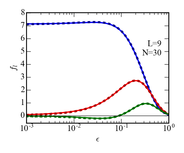
Figure 1: The best estimate of the distribution function, plotted in Legendre components $f_{l}$ for $l=0$ (blue), $l=1$ (red) and $l=2$ (green) for $m/m_{0}=0.1$, $E/n_{2}=12$ Td and $T=293$ K. The result from a Monte-Carlo simulation (thick dashed lines) is shown for comparison.

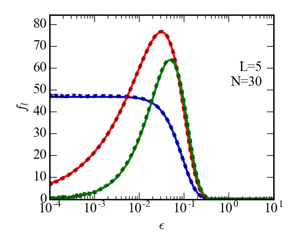
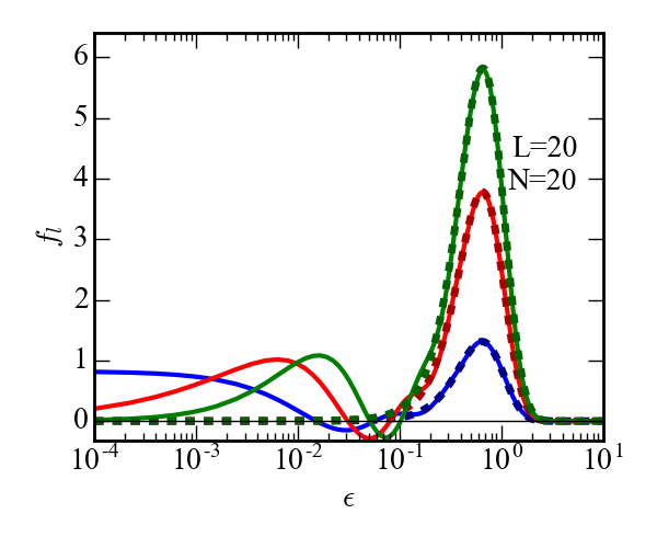
Figure 2: As in figure 1 but for $m/m_{0}=10$ and as a comparison between a) $E/n_{2}=2$ Td and b) $E/n_{2}=12$ Td. When the field is large, the distribution becomes highly non-thermal and the Burnett function expansion cannot reproduce the flat behaviour of the distribution at low energies.

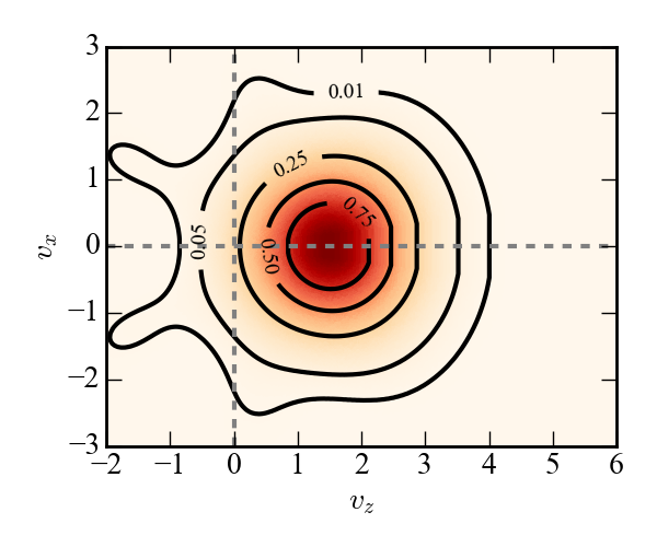
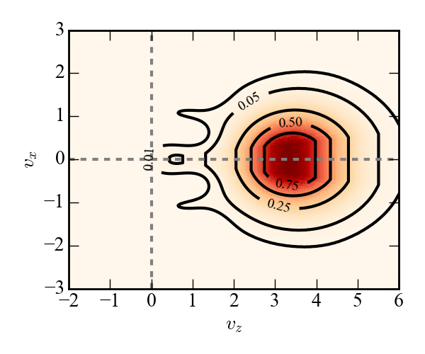
Figure 3: Surface plots of the distribution, $f(v_{x},0,v_{z})$ for $m/m_{0}=10$ and $T=293$ K. In a) $E/n_{2}=2$ Td and the distribution has a resonably strong presence around the origin. In b) $E/n_{2}=12$ Td and the distribution has been significantly shifted away from the origin.

For mass ratios $m/m_{0}\leq 1$, we obtain good agreement between the Boltzmann and MC distribution functions for all fields that we investigated, see figure 1. The agreement between the two calculations continues as the mass ratio becomes larger ($m/m_{0}\leq 2$), however the number of basis functions required to achieve convergence quickly grows. For high fields the convergence in the distribution functions requires many more basis functions than for convergence in the transport quantities alone.

For much larger mass ratios ($m/m_{0}=10$), the Burnett function expansion begins to fail for higher fields, which can be seen in figure 2. In the two different fields shown, $E/n_{2}=2$ and $10$, it can be seen that the main difference in the distribution functions lies in the suppression at low energies. This flat part of the distribution cannot easily be reproduced by the Burnett functions and so the truncation causes the solution to oscillate around in a manner similar to Gibbs phenomena of a Fourier series expansion.

The failure of the Burnett expansion could be expected as the strong fields have significantly distorted the distribution away from a Maxwellian distribution, which is the preferred regime of the Burnett basis. In addition, the peak of the distribution is strongly displaced from the origin, see figure 3, and a Legendre decomposition is not ideal for such distributions. Hence, we believe that a new basis $\psi_{\gamma}(\mathbf{u})$ is required, which does not rely on a spherical harmonic expansion. It would also be desirable for a different basis to more easily handle sharp features in the cross section.

We note that we have also performed $T=0$ calculations which emphasize this conclusion. For $m/m_{0}<1$ and $T=0$, the distributions remain similar enough to a thermal distribution that the Burnett function expansion works well for all field strengths. However, for equal mass ratios and larger, the distribution at $T=0$ becomes highly non-thermal and the Burnett expansion fails for all field strengths. This can be seen in the $\Delta f_{l}$ values shown in table IV.

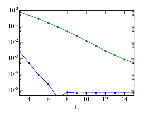
Figure 4: Relative error convergence of drift velocity (blue line) and distribution function ($\Delta f_{0}$, green line), as the number of Legendre polynomials ($L$) is increased. The transport quantity converges much faster than the distribution. Here, $T=293$ K, $m/m_{0}=10$ and $E/n_{2}=10$ Td. The relative error in the drift velocity is taken as the difference in values sampled from a MC simulation. A fixed value of $N=20$, the number of Laugerre polynomials, is used. Note that uncertainties in the MC results place a minimum on the calculate error in the drift velocity.

IV.4 Comments on benchmarking

It is essential to test new code using benchmarks of simple models before applying it to more complicated applications. However, the simple comparisons in this paper highlight a subtlety that can easily give rise to false confirmations for tests on code.

For example, even though the particular case of $m/m_{0}=10$ and $E/n_{2}=12$ Td shown in this paper has clearly not reached convergence in the distribution function, the corresponding transport quantities instead converge quickly. In fact, the distribution has not only not converged, but is nonphysical, with negative values appearing in the distribution. To highlight this, we show in figure 4, the convergence for $E/n_{2}=10$ Td as the truncation in number of Legendre polynomials in increased.

This indicates that benchmarking a transport code by obtaining agreement for transport quantities only in simple models is not sufficient. Proper consideration must be made for the distribution function, especially when an application deviates significantly from the ideal and smooth case of common benchmark models.

There are many examples of processes which may cause a code to break down. Rather than list specific examples, it is instructive to see how an incorrect distribution would affect the results of perturbation theory. Calculating the effect of a perturbation relies on accurate distribution functions in the region where the new process is strongest, e.g. a narrow window of energy, or for a particular pattern in angle. When the distribution function is unphysical, it could even be possible to obtain an incorrect sign of the perturbed quantity.

V Conclusion

We have outlined a general framework to represent the solution of Boltzmann’s equation in the swarm limit, allowing arbitrary basis functions and for arbitrary mass ratios. We have demonstrated how this framework can be applied for the traditional basis set of Burnett functions. We obtained good agreement between our Boltzmann solutions and an independent Monte-Carlo simulation for a large range of parameters.

Although the Burnett function basis always converged quickly in the value of the transport quantities, the distribution functions themselves were only accurately represented for when they are sufficiently close to a thermal Maxwellian distribution. This occurs for $m/m_{0}\geq 1$ and large applied fields. The behaviour of these functions can even be nonphysical, due to negative oscillations in the solutions. This can cause some techniques to fail completely, such as in perturbation theory which makes use of the distributions directly.

This suggests that accurate benchmarking requires models that qualitatively capture the behaviour present in the desired application. Additionally, benchmarks should include the comparison of the complete distribution function.

As we have demonstrated that the spherical harmonic expansion is likely to fail when the peak of the distribution is moved away from the origin, we believe that alternative basis sets should be used. In future work, we will apply and contrast several different basis sets using the framework of section III. In particular, we expect that a basis of B-splines will provide a great deal of flexibility that allows for solutions in cases which have strongly non-thermal distributions.

References

- White and Carlo (2001) R. D. White and M. Carlo, Phys. Rev. E 64, 56409 (2001), URL http://link.aps.org/doi/10.1103/PhysRevE.64.056409.
- Thorn et al. (2009) P. Thorn, L. Campbell, and M. Brunger, PMC Physics B 2, 1 (2009), ISSN 1754-0429, URL http://www.physmathcentral.com/1754-0429/2/1.
- Bruggeman et al. (2016) P. J. Bruggeman, M. J. Kushner, B. R. Locke, J. G. E. Gardeniers, W. G. Graham, D. B. Graves, R. C. H. M. Hofman-Caris, D. Maric, J. P. Reid, E. Ceriani, et al., Plasma Sources Science and Technology 25, 053002 (2016), ISSN 1361-6595, URL http://stacks.iop.org/0963-0252/25/i=5/a=053002?key=crossref.8490978588aa1069ee57bfd0198fc461.
- Boeuf et al. (2013) J.-P. Boeuf, L. L. Yang, and L. C. Pitchford, Journal of Physics D: Applied Physics 46, 015201 (2013), ISSN 0022-3727, URL http://stacks.iop.org/0022-3727/46/i=1/a=015201?key=crossref.289afc7dcabe2690dcd11d66f593162b.
- Mason and McDaniel (1988) E. A. Mason and E. W. McDaniel, Transport Properties of Ions in Gases (Wiley, New York, 1988), ISBN 0471883859.
- Garcia et al. (2011) G. Garcia, Z. L. Petrovic, R. D. White, and S. J. Buckman, IEEE Trans. Plasma Sci. 39, 2962 (2011).
- Salvat et al. (1999) F. Salvat, J. M. Fernández-Varea, J. Sempau, and J. Mazurier, Radiation and environmental biophysics 38, 15 (1999), ISSN 0301-634X, URL http://www.ncbi.nlm.nih.gov/pubmed/10384951.
- Semenenko et al. (2003) V. a. Semenenko, J. E. Turner, and T. B. Borak, Radiation and environmental biophysics 42, 213 (2003), ISSN 0301-634X, URL http://www.ncbi.nlm.nih.gov/pubmed/12920530.
- Markosyan et al. (2015) A. H. Markosyan, J. Teunissen, S. Dujko, and U. Ebert, Plasma Sources Science and Technology 24, 065002 (2015), ISSN 0963-0252, URL http://stacks.iop.org/0963-0252/24/i=6/a=065002?key=crossref.6109bb694c8e30c875a839a09a350941.
- Kumar (1966a) K. Kumar, (null) (1966a).
- Kumar (1967) K. Kumar, (null) (1967).
- Viehland and Mason (1975) L. A. Viehland and E. A. Mason, (null) (1975).
- Kihara (1953) T. Kihara, (null) (1953).
- Kumar and Robson (1973) K. Kumar and R. E. Robson, (null) (1973).
- Lin et al. (1979a) S. L. Lin, L. A. Viehland, and E. A. Mason, (null) (1979a).
- Ness and Viehland (1990) K. F. Ness and L. A. Viehland, (null) (1990).
- White et al. (1999) R. White, K. Ness, and R. Robson, Journal of Physics D: Applied … 32, 1842 (1999), URL http://iopscience.iop.org/0022-3727/32/15/312.
- Viehland (1994) L. A. Viehland, (null) (1994).
- Robson (2006) R. E. Robson, Introductory Transport Theory for Charged Particles in Gases (World Scientific Publishing, Singapore, 2006), ISBN 981-270-011-0.
- Lin et al. (1979b) S. L. Lin, R. E. Robson, and E. A. Mason, (null) (1979b).
- Chapman and Cowling (1970) S. Chapman and T. G. Cowling, The Mathematical Theory of Non-uniform Gases: An Account of the Kinetic Theory of Viscosity, Thermal Conduction and Diffusion in Gases, Cambridge Mathematical Library (Cambridge University Press, 1970), ISBN 9780521408448, URL http://books.google.com.au/books?id=Cbp5JP2OTrwC.
- Pitchford et al. (1981) L. C. Pitchford, S. V. ONeil, and J. R. Rumble, (null) (1981).
- Edmonds (1974) A. R. Edmonds, Angular Momentum in Quantum Mechanics 2nd Edition (Princeton University Press, Princeton, 1974).
- (24) DLMF, NIST Digital Library of Mathematical Functions, http://dlmf.nist.gov/, Release 1.0.13 of 2016-09-16, f. W. J. Olver, A. B. Olde Daalhuis, D. W. Lozier, B. I. Schneider, R. F. Boisvert, C. W. Clark, B. R. Miller and B. V. Saunders, eds., URL http://dlmf.nist.gov/.
- Kumar (1966b) K. Kumar, (null) (1966b).
- White et al. (2009) R. D. White, R. E. Robson, S. Dujko, P. Nicoletopoulos, and B. Li, Journal of Physics D: Applied Physics 42, 194001 (2009), URL http://iopscience.iop.org/0022-3727/42/19/194001.
- Tattersall et al. (2015) W. J. Tattersall, D. G. Cocks, G. J. Boyle, S. J. Buckman, and R. D. White, Phys. Rev. E 91, 43304 (2015), ISSN 1539-3755, URL http://link.aps.org/doi/10.1103/PhysRevE.91.043304.
- Ristivojevic and Petrović (2012) Z. Ristivojevic and Z. L. Petrović, Plasma Sources Science and Technology 21, 035001 (2012).