Shock Dynamics in Stellar Outbursts: I. Shock formation
Abstract
Wave-driven outflows and non-disruptive explosions have been implicated in pre-supernova outbursts, supernova impostors, LBV eruptions, and some narrow-line and superluminous supernovae. To model these events, we investigate the dynamics of stars set in motion by strong acoustic pulses and wave trains, focusing here on nonlinear wave propagation, shock formation, and an early phase of the development of a weak shock. We identify the shock formation radius, showing that a heuristic estimate based on crossing characteristics matches an exact expansion around the wave front and verifying both with numerical experiments. Our general analytical condition for shock formation applies to one-dimensional motions within any static environment, including both eruptions and implosions, and can easily be extended to non-stationary flows. We also consider the early phase of shock energy dissipation. We find that waves of super-Eddington acoustic luminosity always create shocks, rather than damping by radiative diffusion. Therefore, shock formation is integral to super-Eddington outbursts.
1. Introduction
Observational examples of progidious pre-supernova (pre-SN) mass loss now abound. Supernova impostors (Van Dyk & Matheson, 2012) are re-classified as intense luminous blue variable (LBV) outbursts once their progenitors are seen to survive. Some, like SN 2006jc, SN 2009ip, SN 2015bh, and LSQ13zm, undergo one or more eruptions before terminal explosion (Pastorello et al., 2007; Foley et al., 2007; Margutti et al., 2014; Smith et al., 2014; Thöne et al., 2016; Tartaglia et al., 2016). A few percent of core-collapse SNe exhibit narrow lines from dense circumstellar interaction, indicating intense phases of pre-SN mass loss (Smith et al., 2011; Kiewe et al., 2012; Smith, 2014; Moriya et al., 2014). Ofek et al. (2014) find that precursors are common in hydrogen-rich, narrow-line (type IIn) SNe, and Margutti et al. (2016) find evidence for outbursts ejecting in SN 2014C and similar events prior to 10% of type Ibc SNe.
It is not always clear whether each mass-loss episode results from a single shock-driven outburst, an extended wind, or both. However, intense mass-loss is expected in a pre-SN stellar evolution for both low and high progenitor masses. In the low-mass () progenitors of electron-capture SNe, oxygen and silicon shell burning releases a sequence of pulses, building from to ergs over the last year of the star’s life, allowing for the possible ejection of the stellar envelope (Woosley & Heger, 2015). At an order of magnitude higher initial mass (), pulsational pair instability is expected to eject a series of massive shells (Woosley et al., 2007). Outside these mass windows, Quataert & Shiode 2012, Shiode & Quataert 2014, and Smith & Arnett (2014) argue that the enhanced pre-SN mass loss is driven by waves excited in zones of vigorous convection.
Waves deposit their energy by either radiative damping or shock dissipation. Super-Eddington rates of acoustic dissipation can stimulate intense winds like those seen from LBVs and Type IIn SN progenitors. Quataert et al. (2016) envision radiative diffusion as the dominant form of wave dissipation in such events, but as we shall see, shock dissipation is more relevant. Moreover, the existence of 5000 km/s motions around Carinae (Smith, 2008) implies shock driving, as do 2000-7000 km/s speeds in the 2009ip precursor (Foley et al., 2011).
These considerations motivate a detailed investigation of shocks within stars, which we begin here by analyzing the birth and early phase of a radially-propagating shock front. Dessart et al. (2010) has noted that shocks may be responsible for many types of outbursts, and that shocks occur naturally when energy is released over a period shorter than the dynamical time. However, energy is usually released deep within a star where sound speeds are relatively large, so part of the deposited energy must first travel outward as a sound pulse or continuous wave. If the sound is sufficiently intense, it will convert into a shock at some point within the star. Indeed, shocks are a natural outcome of sound propagation. Barring reflection and dissipation by other means, all acoustic waves steepen into shocks in finite time (Landau & Lifshitz, 1959).
Shocks launched by waves from the convective zone have long been considered as a heat source for the solar corona (Biermann, 1946, 1948). Yet, with few exceptions, existing solutions for shock formation and evolution from acoustic waves are restricted to relatively simple cases, such as planar and homogeneous or isothermal atmospheres. We therefore seek more general solutions that can be applied to the stellar problems of interest, although we do consider only one-dimensional flow, such as spherical symmetry.
Spherical symmetry may appear to be a drastic simplification, as the Homunculus nebula, which surrounds the prototypical LBV Car, is strongly bipolar. Moreover, aspherical strong explosions are known to develop strongly non-radial flows near the stellar surface (Matzner et al., 2013; Salbi et al., 2014).
Nevertheless, a thorough understanding of the spherical problem is required for any detailed study of the non-spherical case, so this is where we begin. The spherical idealization was also adopted in numerical investigations by Wyman et al. (2004) and Dessart et al. (2010). It allows us to describe the problem in simple terms: we start with a spherical hydrostatic stellar envelope of enclosed mass , density , pressure , and adiabatic sound speed , where subscript ‘0’ denotes undisturbed quantities, and consider the evolution of an outgoing sound pulse or wave train.
Our ultimate goal is to predict (analytically, if possible) the entire sequence of events set in motion by a strong sound pulse from the stellar interior: its propagation as a sound wave; its steepening into a shock front; its strengthening into a strong shock, and arrival at the stellar surface; and the ensuing ejection and fall-back of matter, and release of light.
The strong-shock phase is pivotal to this sequence, because a normal strong shock must approach the stellar surface like the self-similar solutions identified by Sakurai (1960). In these, the shock velocity follows , for an eigenvalue that depends weakly on the density profile and the post-shock equation of state (Ro & Matzner, 2013). However, to calculate the coefficient to this strong-shock law, and to determine the pattern of shock-deposited heat and momentum, we must first analyze shock formation and strengthening.
We focus here on the precise radius of shock formation at the end of purely acoustic propagation (Phase 1), and provide a simple estimate of the initial phase of shock strengthening in which the wave peak catches up with the shock front (Phase 2). We postpone a detailed examination of shock evolution to a subsequent paper.
We begin, therefore, by reviewing the nature of acoustic pulse propagation, before delving into a detailed analysis of weak shock formation and propagation. We then derive a general expression for the condition of shock formation in two ways. First, we use a wave action principle to generalize a classical derivation based on the crossing of sound front. Then, extending an analysis from the field of sonoluminescence, we use an expansion around the wave front to derive the same result. Numerical simulations validate our result and provide insight into the subsequent phase of weak shock evolution.
2. Propagation of a sound pulse
Let us begin by considering the propagation of a sound pulse, launched outward from the stellar core into the stellar envelope. Any such pulse can be decomposed into normal modes of the stellar envelope, and a pressure mode of angular momentum quantum number and frequency can only propagate through a zone with sound speed , if (e.g., Hansen & Kawaler, 1994). Non-radial modes () thus meet an angular momentum barrier and become evanescent inward of this radius. This suppresses their generation by subsonic motions in the stellar core; we consider only radial motions, for which there is no such barrier.
There is, nevertheless, an outer turning radius for radial sound waves. Close to the stellar surface, where
| (1) |
the density scale height is traversed by sound in a time less than and the atmosphere responds quasi-statically, causing reflection (e.g., Aerts et al., 2010). (For later reference we designate as the local reflection frequency.)
Away from its points of reflection, and in the absence of dissipation, a linear, outwardly-propagating pressure wave carries a constant luminosity . It is worthwhile to understand why and when should be conserved, however; for this we rely on Dewar (1970).
Dewar averaged the Lagrangian of an adiabatic fluid over a wave cycle, arriving at a conservation law for the wave action density
Here is the group velocity ( for sound waves), is the wave energy density, is the wavevector, and is the mean flow velocity. In an otherwise motionless stellar envelope (), is itself conserved, and if is oriented radially outward, then the total wave luminosity
across the area will be constant (along the wave trajectory) as the wave travels. Different outgoing waves may nevertheless carry different values of .
Conservation of wave energy is a familiar feature of WKB theory. Note, however, that the outward wave luminosity is not conserved if: (1) the wave is reflected; (2) the stellar envelope is in motion, so that varies; (3) non-adiabatic effects lead to dissipation that saps the wave energy; or (4) a shock forms, as shocks involve localized dissipation.
The mean wave energy density in a wave with peak velocity is , so the mean wave luminosity in a spherical star is
| (2) |
where
| (3) |
We see immediately that . Since supersonic wave motion () produces a shock very rapidly, sound cannot propagate in zones where – typically, the outer stellar envelope or atmosphere. However, wave dissipation by diffusion or shock formation sets in far before this condition is satisfied. A shock-driven outburst is only possible if diffusion does not sap prior to shock formation, so it is important to examine both processes in detail.
2.1. Thermal diffusion
Our estimate of losses due to thermal diffusion will be approximate, and similar to the analysis by Quataert & Shiode (2012). Below the stellar photosphere, this process is described by the diffusion equation , where is the diffusive flux, is the thermal diffusivity, and is the portion of the total energy density that can diffuse (i.e., the radiation energy density, if diffusion is due to photons). This equation applies to the outward diffusion of luminosity, so
Here is the radiation pressure scale height, and is the diffusive portion of the stellar luminosity , so , where the equality holds in regions that are not convective.
If we consider the change of the wave luminosity along a wave front (phase const.) due to thermal diffusion, then considering that the thermal diffusion time is , we find
Here is the part of the wave luminosity subject to diffusion. Using our expression for , the net loss across a distance is
The last step relies on the relation for an ideal fluid of adiabatic index , and yields a numerical prefactor in the range 0.1 to 0.3.
The form of (2.1) is convenient for determining whether linear acoustic waves will damp or reflect as they approach the stellar surface. However, our purpose is to quantify the non-linear process of shock formation, which we consider next. We return to radiative damping in section 5, where we derive a critical wave luminosity for shock formation.
3. Shock Formation
The evolution of an acoustic wave into a shock has two distinct stages: the creation of the shock discontinuity, and the driving of this shock by the acoustic pulse behind it. If this driving is successful, the shock will become strong and approach the stellar surface in the manner described by Sakurai (1960). We seek to predict the wave evolution through the first and second stages. We first identify the radius at which the shock first forms; for this, we provide both a heuristic and a detailed calculation.
3.1. Shock formation radius: heuristic derivation
For a heuristic derivation of the location of shock formation, consider the fact that acoustical information (such as the value of ) travels along outward-moving sound fronts (or characteristics), and that a shock forms when characteristics arrive at the same location carrying conflicting information. Some variation of the propagation speed is inevitable if is non-uniform, as the scalings of adiabatic linear perturbations (Landau & Lifshitz, 1959; Whitham, 1974) imply
| (5) |
Here represents the perturbation from the background state for a given fluid element. In this section we generalize a classic result (Landau & Lifshitz, 1959, §101) to non-planar and non-uniform environments.
Consider two nearby characteristics launched from an initial radius but separated in space by a small amount at an initial time – or equivalently, separated in time (at a fixed ) by . Each propagates outward at , but they move at different speeds because differs slightly between them. At some larger radius, the difference in arrival times is
The second step uses equation (5), as well as , which is correct to first order in .
We can now employ the conservation of wave luminosity, in the form
If we also write , then after a little algebra we arrive at the shock formation condition
| (6) |
which corresponds to the crossing of characteristics: at .
This is only a heuristic derivation, as we relied on Dewar’s phase-averaged conservation law to infer the constancy of , and from that, the propagation of characteristics within a single wave pulse. This procedure is hardly rigorous. However, we now show that equation (6) coincides perfectly with a more detailed calculation.
3.2. Detailed derivation of shock formation radius
The condition for shock formation from a sound pulse has been worked out in the context of sonoluminescence by Lin & Szeri (2001, hereafter LS01), and the solution is applicable to inertially-confined fusion and related topics. We generalize LS01’s analysis to account for a body force (due to the stellar gravity ) as well as the variations of fluid properties that define the stellar structure.
We begin with the Euler equations,
| (7) | |||||
| (8) | |||||
| (9) |
where the density , pressure , sound speed , and fluid velocity reference the wave properties, and and are partial derivatives with respect to space and time . In addition to the spherical case () we allow for cylindrical and planar cases ( and 0, respectively); in general .
We assume the structure of the quiescent gas is known (i.e., , , ) and permit the quiescent adiabatic index,
| (10) |
to vary across the star: . This allows for a non-uniform composition in gas and radiation. We account for variations in the instantaneous adiabatic index
| (11) |
which differs from as a fluid element is perturbed. We neglect effects from ionization, which may absorb heat.
Taking equations (10) and (11) with the Euler equations (7)-(9), we choose to substitute with to work only with variables , , , and . This generates the following differential equations:
| (12) | |||||
| (13) | |||||
| (14) |
where
| (15) |
and . We assume the body force is independent of perturbations (Cowling’s approximation). The wave travels only in the radial direction, so refraction is ignored.
Whitham (1974) found that a Taylor expansion of fluid properties about the wave front generates a closed system of equations. From these equations, Lin & Szeri found velocity gradient evolution can be described in an explicit and analytic form until shock formation . While much of the following derivation is similar to LS01, we include a body force (eg. gravity), cylindrical wave solutions, and a variable adiabatic index.
The wave front propagates outward (or left to right) at the local quiescent sound speed,
| (16) |
The primes are derivatives with respect to their independent variable. We define a new coordinate variable around the wave front () and expand the fluid variables for :
| (17) | |||||
| (18) | |||||
| (19) | |||||
| (20) |
Integer subscripts represent the number of spatial derivatives taken (e.g., ). Since the wave front is also a node, we use the quiescent gas values for variables with subscript 0. Variables with non-zero subscript are spatial gradients evaluated at the wave front and are functions in only time. Therefore, our notation states and . Note that we assume the quiescent gas is initially static .
Next, we substitute the expanded variables into the set of differential equations (12)-(15). Since the derivatives are with respect to and not , we change the variables to generate a new derivative:
| (21) | |||||
We collect the and terms from each differential equation to obtain eight equations, which are listed in the Appendix. This requires a meticulous account of all variables. Combining these equations together presents a single differential equation about the variable , which measures the wave steepness or gradient, as a function of only the quiescent gas,
| (22) | |||||
This is an example of a Bernoulli equation (Ince, 1956), which has an analytic solution of the form
Although shock formation is a nonlinear process, our Taylor expansion is justified by the fact that the shock forms at the wave node; only the first term appears in this solution. Insofar as the combination tends to be much larger where a wave shocks than where it was launched (at least in the stellar context), it is reasonably accurate to evaluate equation (3.2) with .
Comparison to equation (6) shows that shock formation () occurs precisely where our heuristic analysis predicts (i.e., ). The wave front evolution is defined entirely by the structure of the quiescent gas, initial wave front gradient and location , and not on the wave’s other properties (wavelength, amplitude, etc.). And, our result holds equally well for planar, cylindrical, or spherical symmetry, and for inward as well as outward propagation. Shock formation is used in fields as diverse as the heating of the Solar corona (Osterbrock, 1961), the deflagration-to-detonation transition in type Ia supernovae (Charignon & Chièze, 2013), and sonoluminescence (LS01), among others, so this general result should be widely applicable.
Although shock formation is a purely local process on the most rapidly compressive characteristic, we can relate it to the properties of a larger wave or pulse. Suppose the wave is monochromatic with initial peak velocity amplitude . The peak compression rate is , achieved at the wave node. In our shock formation criterion, the combination is equivalent to ; but this equals elsewhere, so long as the conditions discussed at the start of §2 hold. Condition (6) therefore becomes
| (24) |
is the change of phase angle. In other words, the wave propagates for
radians before producing a shock, where the bracket means a time average along the wave front. The total propagation time is proportional to , so stronger and higher-frequency waves shock earlier.
3.3. Maturation of the shockwave
To estimate the point of intersection between the wave peak and shock front, we derive their respective trajectories. First, suppose a monochromatic wave with luminosity and frequency is led by a compressive edge (i.e., ). The wave peak initially lags behind the wave front by a distance .
The peak propagates with a speed , where is the compressed local sound speed. Assuming properties of the gas do not vary significantly under compression (i.e., constant and ), we can write the compressed sound speed in terms of the peak pressure . The thermodynamic expression of the mean wave energy density allows and to be expressed in terms of conserved wave properties,
With the kinematic expression (2), the speed of the wave peak becomes
| (25) |
Before shock formation (), the wave front simply travels at the local sound speed . For , the exact shock velocity requires numerical calculations to describe the arrival of the remaining wave pulse. We circumvent this calculation by approximating the shock front strength with the wave peak properties (). With the following shock jump condition,
| (26) |
we approximate the shock Mach number to be
| (27) |
Thus, the wave peak and shock front converge at the same location , once
| (28) |
is satisfied.
4. Hydrodynamic Simulations
To test our analytical predictions of shock formation and provide examples of shock evolution and strengthening, we turn to numerical simulations. We construct one-dimensional planar and spherical simulations in FLASH (Fryxell et al., 2000), a hydrodynamic adaptive mesh refinement (AMR) code. All quiescent structures begin in hydrostatic equilibrium with a gravitational acceleration that is independent of fluid perturbations (Cowling’s approximation). All simulations have inner reflecting and outer diode (outflow) boundary conditions. Two structures are considered: a planar isothermal atmosphere and a stellar polytrope. The adiabatic index is held fixed in all of our simulations.
4.1. Planar Earth Atmosphere
For planar shock formation we consider a vertically stratified, initially isothermal atmosphere of gas (FLASH’s default Earth atmosphere) with , in constant gravity. Lengths in this section should be compared to the 8.8 km scale height of the model, although the results can be scaled to any similar atmopshere.
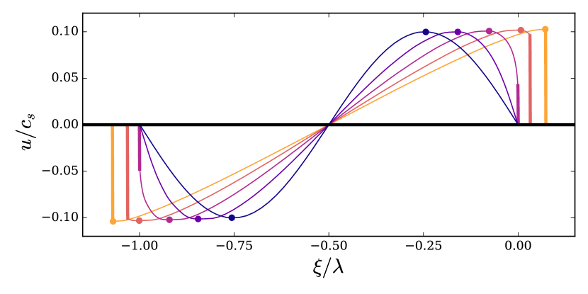
Upward-travelling waves are initialized by setting the isothermal atmosphere out of equilibrium; an example of the initial waveform and its evolution is shown in Figure 1. The initially sinusoidal wave steepens (Phase 1) and forms a shock at the wave node, after which the wave peak approaches (Phase 2) and merges with the shock front.
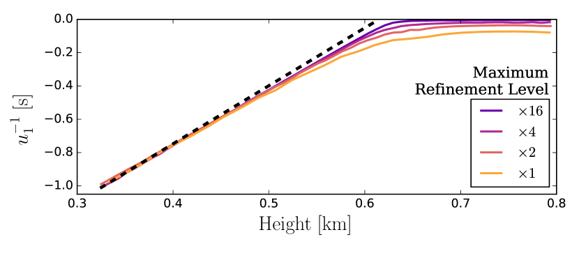
In a grid-based simulation, a shock must span multiple grid cells of length ; for a given velocity jump this sets an upper limit to the compression rate of order . Given this limitation, we expect the numerical solution to converge toward the analytical prediction (eq. 24 as ; this verified in Figure 2 for one set of initial conditions.
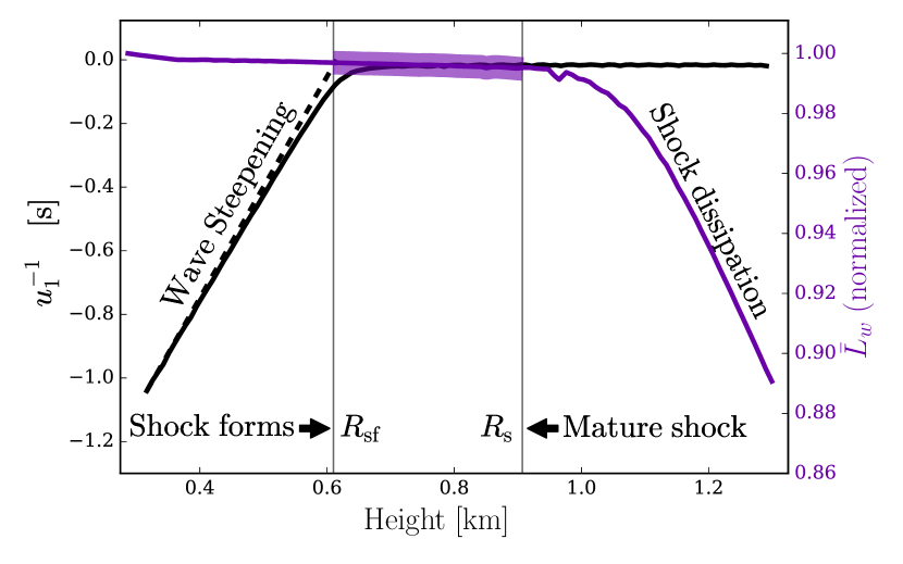
Figure 3 shows that the peak wave luminosity is conserved during the acoustical phase of propagation (Phase 1), just as predicted in Dewar’s theory. Moreover it is diminished by less than 0.5% in the time between shock formation and the arrival of the wave peak at the shock front (Phase 2), and numerical dissipation is responsible for part of this loss.
| Label | (m) | ||
|---|---|---|---|
| A1 | 50 | 0.02 | 2500 |
| A2 | 250 | 0.10 | 2500 |
| B1 | 50 | 0.04 | 1250 |
| B2 | 250 | 0.20 | 1250 |
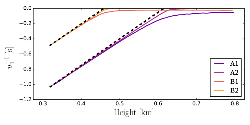
We launch four waves as described in Table 1. Within groups A and B, waves have identical and maximum compression rate. Equation (24) therefore states that waves in each group will steepen identically and form shocks at the same location; this is confirmed in Figure 4a. A1 and B1 have shorter wavelengths and are more poorly resolved, so they obey the analytical prediction more poorly than A2 and B2.

4.2. Spherical Polytropes
We interpolate a polytropic stellar model with a constant adiabatic index of onto a uniform grid of 130,000 cells. We disable AMR, as mesh refinement appeared to stimulate spurious oscillations in regions with short scale heights. We nevertheless observe small oscillations and a weak outflow of matter and corresponding inward-moving rarefaction wave due to imperfect force balance and the outer boundary conditions. (While density and pressure are formally zero at the stellar surface, simulation fluid variables cannot be defined zero. As a result, the grid boundary lies inside the stellar radius.) However, these have negligible impact on our results.
Our initial conditions generated both inward and outward travelling waves, so we measure the outgoing wave properties after it has separated from the ingoing wave. Waves with the shortest wavelength initially span 1% of the domain, contracting to 0.5% of the domain as they traverse regions of lower sound speed. However this is still highly resolved (650 cells). The wave luminosity is conserved to within 1%.
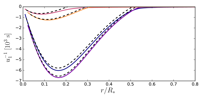
From Figure 5a, we observe equation (24) to successfully predict the location of shock formation for a stellar polytrope in all of our simulations. Our estimate for where the shock fully develops is accurate to within local wavelengths or .
5. Shock dissipation or radiative damping?
The results of the previous sections allow us to quantify which waves dissipate due to radiative damping, and which successfully convert into shocks. Returning to equation (29), we can define at each radius the critical frequency for the wave that damps by radiative diffusion in a single radiation pressure scale height:
| (29) |
the instantaneous damping time due to diffusion is . We can also write the shock formation criterion where . Evaluating the ratio of diffusion time to shock time at frequency ,
| (30) |
This analysis indicates a shock forms before radiative damping has had time to act, for any waves more luminous than the stellar radiative luminosity. Therefore, wave-driven outbursts that exceed the envelope Eddington luminosity must involve shock formation. This is especially true for super-Eddington outbursts, as the quiescent luminosity is usually well below the envelope’s Eddington limit.
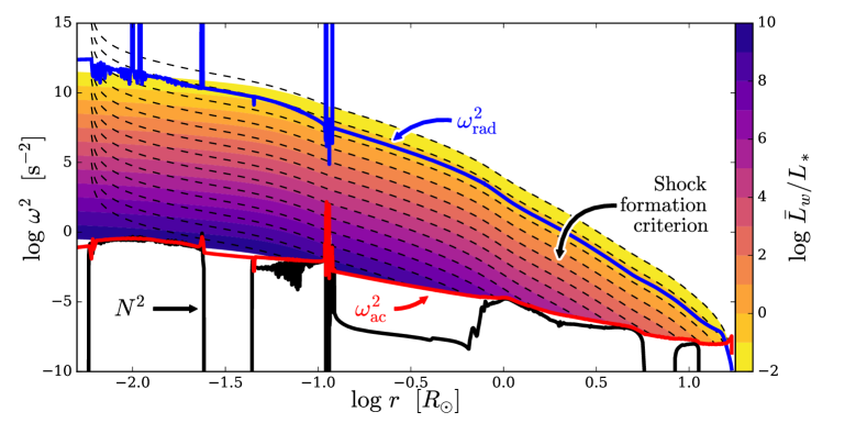
In figure (6) we examine acoustic propagation, radiative damping, and shock formation within a model star generated by the MESA code (r8118) from an initial solar-metallicity object of 50 . At the time of the figure, stellar winds have removed all but and core oxygen burning has just begun. We plot the Brunt-Väisälä (), acoustic cutoff (), and radiative damping frequencies (), as well as the shock formation radius (eq. 24). As is clear from the figure, shock formation outpaces radiative damping for , somewhat below the stellar luminosity of .
6. Discussion
In this work we have found that strong stellar outbursts and wave-driven outflows necessarily involve shock formation, rather than radiative dissipation. The distinction is important because shock formation occurs at a different radius and deposits wave energy in a distributed fashion, and can lead to mass ejection at the surface.
Moreover, we find that the condition for shock formation within stars can be predicted with a single expression (equation 24). This result is remarkably general, as it applies to any one-dimensional motion within a non-isentropic fluid; yet it is almost as simple as the classic result for planar, isentropic flows. Our exact derivation, which we obtained by generalizing an analysis from the sonoluminescence literature (Lin & Szeri, 2001), matches a heuristic calculation of wave crossings that using wave luminosity conservation (which can be considered a consequence of the wave action principle due to Dewar 1970, in the absence of reflections).
Because of its generality, our result applies equally well to a single wave pulse and to a continuous wave. Furthermore, the formation of a shock from one wave tends to be unaffected by the passage of earlier waves, because these typically deposit energy and momentum only after they have steepened into shocks. Therefore our criterion for shock formation remains reasonably valid even within stars that have been set into motion by a strong pulse or a steady acoustical flux.
Our next task is to predict in detail the propagation of weak shocks outside the shock formation radius, in order to understand the transition from weak to strong and to determine the patterns of heat and momentum deposition. We shall address this in subsequent papers.
Appendix A Taylor expansion around a wave node
Substituting the Taylor expanded fluid variables into the fluid equations generates the following collection of and order terms. Note that we simplify the notation by substituting .
| (A2) | |||||||
| (A4) | |||||||
| (A6) | |||||||
| (A8) |
We leave out the result from the continuity equation (A2) since it is egregious in length and not used in the next derivation. The variables that emerge in (A2) include , , , , , , and .
Appendix B Derivation
The goal is to find a final differential equation with , and any quiescent variables (subscript 0). Through a process of elimination using equations (A3), (A4), (A6), and the derivative of (A3), one can generate the following differential equation:
| (B1) |
The quiescent gas is initially in hydrostatic equilibrium, which satisfies . Since the local quiescent sound speed is , we can eliminate the body force (i.e., gravity) by substituting .
With respect to , this equation is known as the Bernoulli equation for . The solution can be written explicitly in the form
| (B2) |
where,
We can rewrite the integrand in terms of the radius, since , and integrate the expression to obtain
| (B3) |
Thus, the wave front evolution can be solved analytically with the following expression
Notice that the body force is never defined explicitly. Since is arbitrary, the analytic result must be valid for an arbitrary distribution of fluid. It is also applicable for waves in planar, cylindrical, and spherical symmetry ( 0, 1, 2).
References
- Aerts et al. (2010) Aerts, C., Christensen-Dalsgaard, J., & Kurtz, D. W. 2010, Asteroseismology
- Biermann (1946) Biermann, L. 1946, Naturwissenschaften, 33, 118
- Biermann (1948) —. 1948, ZAp, 25, 161
- Charignon & Chièze (2013) Charignon, C., & Chièze, J.-P. 2013, A&A, 550, A105
- Dessart et al. (2010) Dessart, L., Livne, E., & Waldman, R. 2010, MNRAS, 405, 2113
- Dewar (1970) Dewar, R. L. 1970, Physics of Fluids, 13, 2710
- Foley et al. (2011) Foley, R. J., Berger, E., Fox, O., et al. 2011, ApJ, 732, 32
- Foley et al. (2007) Foley, R. J., Smith, N., Ganeshalingam, M., et al. 2007, ApJ, 657, L105
- Fryxell et al. (2000) Fryxell, B., Olson, K., Ricker, P., et al. 2000, The Astrophysical Journal Supplement Series, 131, 273.
- Hansen & Kawaler (1994) Hansen, C. J., & Kawaler, S. D. 1994, Stellar Interiors. Physical Principles, Structure, and Evolution., 84
- Ince (1956) Ince, E. 1956, Ordinary Differential Equations, Dover Books on Mathematics (Dover Publications).
- Kiewe et al. (2012) Kiewe, M., Gal-Yam, A., Arcavi, I., et al. 2012, ApJ, 744, 10
- Landau & Lifshitz (1959) Landau, L. D., & Lifshitz, E. M. 1959, Fluid mechanics
- Lin & Szeri (2001) Lin, H., & Szeri, A. J. 2001, Journal of Fluid Mechanics, 431, 161.
- Margutti et al. (2014) Margutti, R., Milisavljevic, D., Soderberg, A. M., et al. 2014, The Astrophysical Journal, 780, 21.
- Margutti et al. (2016) Margutti, R., Kamble, A., Milisavljevic, D., et al. 2016, ArXiv e-prints, arXiv:1601.06806
- Matzner et al. (2013) Matzner, C. D., Levin, Y., & Ro, S. 2013, ApJ, 779, 60
- Moriya et al. (2014) Moriya, T. J., Maeda, K., Taddia, F., et al. 2014, MNRAS, 439, 2917
- Ofek et al. (2014) Ofek, E. O., Sullivan, M., Shaviv, N. J., et al. 2014, The Astrophysical Journal, 789, 104.
- Osterbrock (1961) Osterbrock, D. E. 1961, ApJ, 134, 347
- Pastorello et al. (2007) Pastorello, A., Smartt, S. J., Mattila, S., et al. 2007, Nature, 447, 829
- Quataert et al. (2016) Quataert, E., Fernández, R., Kasen, D., Klion, H., & Paxton, B. 2016, MNRAS, 458, 1214
- Quataert & Shiode (2012) Quataert, E., & Shiode, J. 2012, MNRAS, 423, L92
- Ro & Matzner (2013) Ro, S., & Matzner, C. D. 2013, ApJ, 773, 79
- Sakurai (1960) Sakurai, A. 1960, Communications on Pure and Applied Mathematics, 13, 353.
- Salbi et al. (2014) Salbi, P., Matzner, C. D., Ro, S., & Levin, Y. 2014, ApJ, 790, 71
- Shiode & Quataert (2014) Shiode, J. H., & Quataert, E. 2014, ApJ, 780, 96
- Smith (2008) Smith, N. 2008, Nature, 455, 201
- Smith (2014) —. 2014, ARA&A, 52, 487
- Smith & Arnett (2014) Smith, N., & Arnett, W. D. 2014, ApJ, 785, 82
- Smith et al. (2011) Smith, N., Li, W., Filippenko, A. V., & Chornock, R. 2011, MNRAS, 412, 1522
- Smith et al. (2014) Smith, N., Mauerhan, J. C., & Prieto, J. L. 2014, MNRAS, 438, 1191
- Tartaglia et al. (2016) Tartaglia, L., Pastorello, A., Sullivan, M., et al. 2016, MNRAS, 459, 1039
- Thöne et al. (2016) Thöne, C. C., de Ugarte Postigo, A., Leloudas, G., et al. 2016, ArXiv e-prints, arXiv:1606.09025
- Van Dyk & Matheson (2012) Van Dyk, S. D., & Matheson, T. 2012, in Astrophysics and Space Science Library, Vol. 384, Eta Carinae and the Supernova Impostors, ed. K. Davidson & R. M. Humphreys, 249
- Whitham (1974) Whitham, G. 1974, Linear and Nonlinear Waves (Wiley).
- Woosley et al. (2007) Woosley, S. E., Blinnikov, S., & Heger, A. 2007, Nature, 450, 390
- Woosley & Heger (2015) Woosley, S. E., & Heger, A. 2015, ApJ, 810, 34
- Wyman et al. (2004) Wyman, M. C., Chernoff, D. F., & Wasserman, I. 2004, MNRAS, 354, 1053