Characterizing solar-type stars from full-length Kepler data sets using the Asteroseismic Modeling Portal

The Kepler space telescope yielded unprecedented data for the study of solar-like oscillations in other stars. The large samples of multi-year observations posed an enormous data analysis challenge that has only recently been surmounted. Asteroseismic modeling has become more sophisticated over time, with better methods gradually developing alongside the extended observations and improved data analysis techniques. We apply the latest version of the Asteroseismic Modeling Portal (AMP) to the full-length Kepler data sets for 57 stars, comprising planetary hosts, binaries, solar-analogs, active stars, and for validation purposes, the Sun. From an analysis of the derived stellar properties for the full sample, we identify a variation of the mixing-length parameter with atmospheric properties. We also derive a linear relation between the stellar age and a characteristic frequency separation ratio. In addition, we find that the empirical correction for surface effects suggested by Kjeldsen and coworkers is adequate for solar-type stars that are not much hotter ($T_{\rm eff}$ $\lesssim 6200$ K) or significantly more evolved ($\log g$ $\gtrsim 4.2$, $\langle\Delta\nu\rangle$ $\gtrsim 80\mu$Hz) than the Sun. Precise parallaxes from the Gaia mission and future observations from TESS and PLATO promise to improve the reliability of stellar properties derived from asteroseismology.

1 Introduction

Table 1: Spectroscopic constraints and complementary data of the Kepler targets

KIC ID	$T_{\rm eff}$	[M/H]	$K_{s}$	$A_{K_{S}}$	PROT	Ref.
	(K)	(dex)	(mag)	(mag)	(days)
1435467	6326 $\pm$ 77	$+$0.01 $\pm$ 0.10	7.718 $\pm$ 0.009	0.011 $\pm$ 0.004	6.68 $\pm$ 0.89	1,A
2837475	6614 $\pm$ 77	$+$0.01 $\pm$ 0.10	7.464 $\pm$ 0.023	0.008 $\pm$ 0.002	3.68 $\pm$ 0.36	1,A
3427720	6045 $\pm$ 77	$-$0.06 $\pm$ 0.10	7.826 $\pm$ 0.009	0.020 $\pm$ 0.019	13.94 $\pm$ 2.15	1,B
3656476	5668 $\pm$ 77	$+$0.25 $\pm$ 0.10	8.008 $\pm$ 0.014	0.022 $\pm$ 0.050	31.67 $\pm$ 3.53	1,A
3735871	6107 $\pm$ 77	$-$0.04 $\pm$ 0.10	8.477 $\pm$ 0.016	0.018 $\pm$ 0.027	11.53 $\pm$ 1.24	1,A
4914923	5805 $\pm$ 77	$+$0.08 $\pm$ 0.10	7.935 $\pm$ 0.017	0.017 $\pm$ 0.029	20.49 $\pm$ 2.82	1,A
5184732	5846 $\pm$ 77	$+$0.36 $\pm$ 0.10	6.821 $\pm$ 0.005	0.012 $\pm$ 0.007	19.79 $\pm$ 2.43	1,A
5950854	5853 $\pm$ 77	$-$0.23 $\pm$ 0.10	9.547 $\pm$ 0.017	0.002 $\pm$ 0.004		1
6106415	6037 $\pm$ 77	$-$0.04 $\pm$ 0.10	5.829 $\pm$ 0.017	0.003 $\pm$ 0.020		1
6116048	6033 $\pm$ 77	$-$0.23 $\pm$ 0.10	7.121 $\pm$ 0.009	0.013 $\pm$ 0.020	17.26 $\pm$ 1.96	1,A
6225718	6313 $\pm$ 76	$-$0.07 $\pm$ 0.10	6.283 $\pm$ 0.011	0.003 $\pm$ 0.001		1
6603624	5674 $\pm$ 77	$+$0.28 $\pm$ 0.10	7.566 $\pm$ 0.019	0.008 $\pm$ 0.008		1
6933899	5832 $\pm$ 77	$-$0.01 $\pm$ 0.10	8.171 $\pm$ 0.015	0.023 $\pm$ 0.017		1
7103006	6344 $\pm$ 77	$+$0.02 $\pm$ 0.10	7.702 $\pm$ 0.015	0.007 $\pm$ 0.010	4.62 $\pm$ 0.48	1,A
7106245	6068 $\pm$ 102	$-$0.99 $\pm$ 0.19	9.419 $\pm$ 0.006	0.015 $\pm$ 0.029		4
7206837	6305 $\pm$ 77	$+$0.10 $\pm$ 0.10	8.575 $\pm$ 0.011	0.004 $\pm$ 0.005	4.04 $\pm$ 0.28	1,A
7296438	5775 $\pm$ 77	$+$0.19 $\pm$ 0.10	8.645 $\pm$ 0.009	0.012 $\pm$ 0.018	25.16 $\pm$ 2.78	1,A
7510397	6171 $\pm$ 77	$-$0.21 $\pm$ 0.10	6.544 $\pm$ 0.009	0.018 $\pm$ 0.010		1
7680114	5811 $\pm$ 77	$+$0.05 $\pm$ 0.10	8.673 $\pm$ 0.006	0.011 $\pm$ 0.013	26.31 $\pm$ 1.86	1,A
7771282	6248 $\pm$ 77	$-$0.02 $\pm$ 0.10	9.532 $\pm$ 0.010	0.005 $\pm$ 0.001	11.88 $\pm$ 0.91	1,A
7871531	5501 $\pm$ 77	$-$0.26 $\pm$ 0.10	7.516 $\pm$ 0.017	0.023 $\pm$ 0.021	33.72 $\pm$ 2.60	1,A
7940546	6235 $\pm$ 77	$-$0.20 $\pm$ 0.10	6.174 $\pm$ 0.011	0.023 $\pm$ 0.009	11.36 $\pm$ 0.95	1,A
7970740	5309 $\pm$ 77	$-$0.54 $\pm$ 0.10	6.085 $\pm$ 0.011	0.003 $\pm$ 0.013	17.97 $\pm$ 3.09	1,A
8006161	5488 $\pm$ 77	$+$0.34 $\pm$ 0.10	5.670 $\pm$ 0.015	0.009 $\pm$ 0.006	29.79 $\pm$ 3.09	1,A
8150065	6173 $\pm$ 101	$-$0.13 $\pm$ 0.15	9.457 $\pm$ 0.014	0.010 $\pm$ 0.013		4
8179536	6343 $\pm$ 77	$-$0.03 $\pm$ 0.10	8.278 $\pm$ 0.009	0.005 $\pm$ 0.016	24.55 $\pm$ 1.61	1,A
8379927	6067 $\pm$ 120	$-$0.10 $\pm$ 0.15	5.624 $\pm$ 0.011	0.004 $\pm$ 0.012	16.99 $\pm$ 1.35	2,A
8394589	6143 $\pm$ 77	$-$0.29 $\pm$ 0.10	8.226 $\pm$ 0.016	0.013 $\pm$ 0.010		1
8424992	5719 $\pm$ 77	$-$0.12 $\pm$ 0.10	8.843 $\pm$ 0.011	0.016 $\pm$ 0.018		1
8694723	6246 $\pm$ 77	$-$0.42 $\pm$ 0.10	7.663 $\pm$ 0.007	0.003 $\pm$ 0.001		1
8760414	5873 $\pm$ 77	$-$0.92 $\pm$ 0.10	8.173 $\pm$ 0.009	0.016 $\pm$ 0.012		1
8938364	5677 $\pm$ 77	$-$0.13 $\pm$ 0.10	8.636 $\pm$ 0.016	0.003 $\pm$ 0.009		1
9025370	5270 $\pm$ 180	$-$0.12 $\pm$ 0.18	7.372 $\pm$ 0.025	0.041 $\pm$ 0.030		3
9098294	5852 $\pm$ 77	$-$0.18 $\pm$ 0.10	8.364 $\pm$ 0.009	0.011 $\pm$ 0.021	19.79 $\pm$ 1.33	1,A
9139151	6302 $\pm$ 77	$+$0.10 $\pm$ 0.10	7.952 $\pm$ 0.014	0.002 $\pm$ 0.011	10.96 $\pm$ 2.22	1,B
9139163	6400 $\pm$ 84	$+$0.15 $\pm$ 0.09	7.231 $\pm$ 0.007	0.013 $\pm$ 0.007		6
9206432	6538 $\pm$ 77	$+$0.16 $\pm$ 0.10	8.067 $\pm$ 0.013	0.032 $\pm$ 0.037	8.80 $\pm$ 1.06	1,A
9353712	6278 $\pm$ 77	$-$0.05 $\pm$ 0.10	9.607 $\pm$ 0.011	0.011 $\pm$ 0.010	11.30 $\pm$ 1.12	1,A
9410862	6047 $\pm$ 77	$-$0.31 $\pm$ 0.10	9.375 $\pm$ 0.013	0.011 $\pm$ 0.001	22.77 $\pm$ 2.37	1,A
9414417	6253 $\pm$ 75	$-$0.13 $\pm$ 0.10	8.407 $\pm$ 0.009	0.010 $\pm$ 0.010	10.68 $\pm$ 0.66	7,A
9955598	5457 $\pm$ 77	$+$0.05 $\pm$ 0.10	7.768 $\pm$ 0.017	0.002 $\pm$ 0.001	34.20 $\pm$ 5.64	1,A
9965715	5860 $\pm$ 180	$-$0.44 $\pm$ 0.18	7.873 $\pm$ 0.012	0.005 $\pm$ 0.005		3
10079226	5949 $\pm$ 77	$+$0.11 $\pm$ 0.10	8.714 $\pm$ 0.012	0.015 $\pm$ 0.025	14.81 $\pm$ 1.23	1,A
10454113	6177 $\pm$ 77	$-$0.07 $\pm$ 0.10	7.291 $\pm$ 9.995	0.042 $\pm$ 0.019	14.61 $\pm$ 1.09	1,A
10516096	5964 $\pm$ 77	$-$0.11 $\pm$ 0.10	8.129 $\pm$ 0.015	0.000 $\pm$ 0.012		1
10644253	6045 $\pm$ 77	$+$0.06 $\pm$ 0.10	7.874 $\pm$ 0.021	0.008 $\pm$ 0.015	10.91 $\pm$ 0.87	1,A
10730618	6150 $\pm$ 180	$-$0.11 $\pm$ 0.18	7.874 $\pm$ 0.021	0.008 $\pm$ 0.015		3
10963065	6140 $\pm$ 77	$-$0.19 $\pm$ 0.10	7.486 $\pm$ 0.011	0.003 $\pm$ 0.016	12.58 $\pm$ 1.70	1,A
11081729	6548 $\pm$ 82	$+$0.11 $\pm$ 0.10	7.973 $\pm$ 0.011	0.005 $\pm$ 0.001	2.74 $\pm$ 0.31	1,A
11253226	6642 $\pm$ 77	$-$0.08 $\pm$ 0.10	7.459 $\pm$ 0.007	0.017 $\pm$ 0.013	3.64 $\pm$ 0.37	1,A
11772920	5180 $\pm$ 180	$-$0.09 $\pm$ 0.18	7.981 $\pm$ 0.014	0.008 $\pm$ 0.005		3
12009504	6179 $\pm$ 77	$-$0.08 $\pm$ 0.10	8.069 $\pm$ 0.019	0.005 $\pm$ 0.034	9.39 $\pm$ 0.68	1,A
12069127	6276 $\pm$ 77	$+$0.08 $\pm$ 0.10	9.494 $\pm$ 0.012	0.016 $\pm$ 0.005	0.92 $\pm$ 0.05	1,A
12069424	5825 $\pm$ 50	$+$0.10 $\pm$ 0.03	4.426 $\pm$ 0.009	0.005 $\pm$ 0.006	23.80 $\pm$ 1.80	5,B
12069449	5750 $\pm$ 50	$+$0.05 $\pm$ 0.02	4.651 $\pm$ 0.005	0.005 $\pm$ 0.006	23.20 $\pm$ 6.00	5,B
12258514	5964 $\pm$ 77	$+$-0.00 $\pm$ 0.10	6.758 $\pm$ 0.011	0.021 $\pm$ 0.021	15.00 $\pm$ 1.84	1,A
12317678	6580 $\pm$ 77	$-$0.28 $\pm$ 0.10	7.631 $\pm$ 0.009	0.027 $\pm$ 0.021		1

Spectroscopic references: ¹Buchhave & Latham (2015), ²Ramírez et al. (2009), ³Pinsonneault et al. (2012), ⁴Huber et al. (2013), ⁵Chaplin et al. (2014), ⁶Pinsonneault et al. (2014),⁷Casagrande et al. (2014)
Rotation period references: ^AGarcía et al. (2014), ^BCeillier et al. (2016)

Figure 1: Normalized posterior probability functions for KIC 12069424. From left to right we show radius, mass, and age. We also show the adopted parameter $\langle P\rangle$ (dashed line), the 68% region (shaded) and $P_{\rm AMP}$ (dotted line).

Solar-like oscillations are stochastically excited and intrinsically damped by turbulent motions in the near-surface layers of stars with substantial outer convection zones. The sound waves produced by these motions travel through the interior of the star, and those with resonant frequencies drive global oscillations that modulate the integrated brightness of the star by a few parts per million and change the surface radial velocity by several meters per second. The characteristic timescale of these variations is determined by the sound travel time across the stellar diameter, which is around 5 minutes for a star like the Sun. With sufficient precision, more than a dozen consecutive overtones can be detected for each set of oscillation modes with radial, dipole, quadrupole, and sometimes even octupole geometry (i.e., for $l=0,1,2,$ and 3, respectively, where $l$ is the angular degree). The technique of asteroseismology uses these oscillation frequencies combined with other observational constraints to measure the stellar radius, mass, age, and other properties of the stellar interior (for a recent review, see Chaplin & Miglio 2013).

The Kepler space telescope yielded unprecedented data for the study of solar-like oscillations in other stars. Ground-based radial velocity data had previously allowed the detection of solar-like oscillations in some of the brightest stars in the sky (e.g., Brown et al. 1991; Kjeldsen et al. 1995; Bedding et al. 2001; Bouchy & Carrier 2002; Carrier & Bourban 2003), but intensive multi-site campaigns were required to measure and identify the frequencies unambiguously (e.g., Arentoft et al. 2008). The Convection Rotation and planetary Transits satellite (CoRoT, Baglin et al. 2006) achieved the photometric precision necessary to detect solar-like oscillations in main-sequence stars (e.g., Michel et al. 2008), and it obtained continuous photometry for up to five months. NASA’s Kepler mission (Borucki et al. 2010) extended these initial successes to a larger sample of solar-type stars, with observations eventually spanning up to several years (Chaplin et al. 2010). Precise photometry from Kepler led to the detection of solar-like oscillations in nearly 600 main-sequence and subgiant stars (Chaplin et al. 2014), including the measurement of individual frequencies in more than 150 targets (Appourchaux et al. 2012; Davies et al. 2016; Lund et al. 2017).

Asteroseismic modeling has become more sophisticated over time, with better methods gradually developing alongside the extended observations and improved data analysis techniques. Initial efforts attempted to reproduce the observed large and small frequency separations with models that simultaneously matched constraints from spectroscopy (e.g., Christensen-Dalsgaard et al. 1995; Thévenin et al. 2002; Fernandes & Monteiro 2003; Thoul et al. 2003). As individual oscillation frequencies became available, modelers started to match the observations in échelle diagrams that highlighted variations around the average frequency separations (e.g., Di Mauro et al. 2003; Guenther & Brown 2004; Eggenberger et al. 2004). This approach continued until the frequency precision from longer space-based observations became sufficient to reveal systematic errors in the models that are known as surface effects, which arise from incomplete modeling of the near-surface layers where the mixing-length treatment of convection is approximate. Kjeldsen et al. (2008) proposed an empirical correction for the surface effects based on the discrepancy for the standard solar model, and applied it to ground-based observations of several stars with different masses and evolutionary states. The correction was subsequently implemented using stars observed by CoRoT and Kepler (Kallinger et al. 2010; Metcalfe et al. 2010).

During the Kepler mission, asteroseismic modeling methods were adapted as longer data sets became available. The first year of short-cadence data (sampled at 58.85 s, Gilliland et al. 2010) was devoted to an asteroseismic survey of 2000 solar-type stars observed for one month each. The survey initially yielded frequencies for 22 stars, allowing detailed modeling (Mathur et al. 2012), and hundreds of targets were flagged for extended observations during the remainder of the mission. Longer data sets improved the signal-to-noise ratio (S/N) of the power spectrum for stars with previously marginal detections, and yielded additional oscillation frequencies for the best targets in the sample. The first coordinated analysis of nine-month data sets yielded individual frequencies in 61 stars (Appourchaux et al. 2012), though many were subgiants with complex patterns of dipole mixed-modes. The larger set of radial orders observed in each star began to reveal the limitations of the empirical correction for surface effects (Metcalfe et al. 2014). This situation motivated the implementation of a Bayesian method that marginalized over the unknown systematic error for each frequency (Gruberbauer et al. 2012), as well as a method for fitting ratios of frequency separations that are insensitive to surface effects (Roxburgh & Vorontsov 2003; Bazot 2013; Silva Aguirre et al. 2013). It also inspired the development of a more physically motivated correction based on an analysis of frequency shifts induced by the solar magnetic cycle (Gough 1990; Ball & Gizon 2014; Schmitt & Basu 2015). The Kepler telescope completed its primary mission in 2013, but the large samples of multi-year observations posed an enormous data analysis challenge that has only recently been surmounted (Benomar et al. 2014a, b; Davies et al. 2015, 2016; Lund et al. 2017). The first modeling of these full-length data sets appeared in Silva Aguirre et al. (2015) and Metcalfe et al. (2015).

In this paper we apply the latest version of the Asteroseismic Modeling Portal (hereafter AMP, see Metcalfe et al. 2009) to oscillation frequencies derived from the full-length Kepler observations for 57 stars, as determined by Lund et al. (2017). The new fitting method relies on ratios of frequency separations rather than the individual frequencies, so that we can use the modeling results to investigate the empirical amplitude and character of the surface effects within the sample. We describe the sources of our adopted observational constraints in Section 2. We outline updates to the AMP input physics and fitting methods in Section 3, including an overview of how the optimal stellar properties and their uncertainties are determined. In Section 4 we present the modeling results, and in Section 5 we use them to establish the limitations of the Kjeldsen et al. (2008) correction for surface effects. Finally, after summarizing in Section 6, we discuss our expectations for asteroseismic modeling of future observations from the Transiting Exoplanet Survey Satellite, (TESS, Ricker et al. 2015) and PLanetary Transits and Oscillations of stars (PLATO, Rauer et al. 2014) missions.

2 Observational constraints

To constrain the properties of each star in our sample, we adopted the solar-like oscillation frequencies determined by Lund et al. (2017) from a uniform analysis of the full-length Kepler data sets. For each target, the power spectrum of the time-series photometry shows the oscillations embedded in several background components attributed to granulation, faculae, and shot noise. The power spectral distribution of individual modes were modeled as Lorentzian functions, and the background components were optimized simultaneously in a Bayesian manner using the procedure described in Lund et al. (2014). For the targets presented here, this analysis resulted in sets of oscillation modes spanning 7 to 20 radial orders. In most cases, the identified frequencies included only $l=0$, 1, and 2 modes, but for 14 stars, the mode-fitting procedure also identified limited sets of $l=3$ modes spanning 2 to 6 radial orders. Complete tables of the identified frequencies for each star are published in Lund et al. (2017).

To complement the oscillation frequencies, we also adopted spectroscopic constraints on the effective temperature, $T_{\rm eff}$, and metallicity, [M/H], for each star. For 46 of the targets in our sample, we used the uniform spectroscopic analysis of Buchhave & Latham (2015). In this case, the values and uncertainties on $T_{\rm eff}$ and [M/H] were determined using the Stellar Parameters Classification (SPC) method described in detail by Buchhave et al. (2012, 2014). For the other 11 stars in our sample, which were not included in Buchhave & Latham (2015), we adopted constraints from a variety of sources, including Ramírez et al. (2009); Pinsonneault et al. (2012); Huber et al. (2013); Chaplin et al. (2014); Pinsonneault et al. (2014), and from the SAGA survey (Casagrande et al. 2014). The 57 stars in our sample span a range of $T_{\rm eff}$ from 5180 to 6642 K and [M/H] from $-$0.99 to 0.36 dex. These atmospheric constraints are listed in Table 1 along with the K-band magnitude from 2MASS, $K_{s}$ (Skrutskie et al. 2006), the derived interstellar absorption, $A_{Ks}$ (see Section 4.2), and rotational periods from García et al. (2014) and Ceillier et al. (2016). Although independent determinations of the radius and luminosity are available for a few of the stars in our sample, we excluded these constraints from the modeling so that we could use them to assess the accuracy of our results (see Section 4).

Table 2: Reference solar parameters from AMP using the updated method and physics

	AMP1	AMP2	AMP3	AMP4	$\langle P\rangle$	$\sigma$
$R$ (R⊙)	1.002	1.003	1.003	1.010	1.001	0.005
$M$ (M⊙)	1.01	1.01	1.01	1.03	1.001	0.02
Age (Gyr)	4.59	4.38	4.41	4.69	4.38	0.22
$Z_{i}$	0.019	0.021	0.020	0.024	0.017	0.002
$Y_{i}$	0.266	0.281	0.278	0.282	0.265	0.023
$\alpha$	2.16	2.24	2.24	2.30	2.12	0.12
$L$ (L⊙)	0.96	0.99	0.99	1.00	0.97	0.03
$\log g$ (dex)	4.441	4.439	4.439	4.442	4.438	0.003
$\chi^{2}$	1.047	0.968	0.995	1.058

Figure 2: HR diagram showing the position of the sample of stars used for this work. Evolutionary tracks for solar-metallicity models with 1.0, 1.2, and 1.4 M_⊙ stellar masses are shown.

3 Asteroseismic modeling

Based on the observational constraints described in Section 2, we determined the properties of each star in our sample using the latest version of AMP. The method relies on a parallel genetic algorithm (hereafter GA, see Metcalfe & Charbonneau 2003) to optimize the match between the properties of a stellar model and a given set of observations. The asteroseismic models are generated by the Aarhus stellar evolution and adiabatic pulsation codes (Christensen-Dalsgaard 2008b, a). The search procedure generates thousands of models that can be used to evaluate the stellar properties and their uncertainties. Unlike the usual grid-modeling approach, the GA preferentially samples combinations of model parameters that provide a better than average match to the observations. This approach allows us not only to identify the globally optimal solution, but also to include the effects of parameter correlations and non-uniqueness into reliable uncertainties. Below we outline recent updates to the input physics and model-fitting methods, and we describe improvements to our statistical analysis of the results.

3.1 Updated physics and methods

The AMP code has been in development since 2004. Details about previous versions are outlined in Metcalfe et al. (2015). For this paper we use version 1.3, which includes input physics that are mostly unchanged from version 1.2 (Metcalfe et al. 2014). It uses the 2005 release of the OPAL equation of state (Rogers & Nayfonov 2002), with opacities from OPAL (Iglesias & Rogers 1996) supplemented by Ferguson et al. (2005) at low temperatures. Nuclear reaction rates come from the NACRE collaboration (Angulo et al. 1999). The prescription of Michaud & Proffitt (1993) for diffusion and settling is applied to helium, but not to heavier elements because some models are numerically instable. Convection is described using the mixing-length treatment of Böhm-Vitense (1958) with no overshoot.

There have been several minor updates to the model physics for version 1.3 of the AMP code. First, it incorporates the revised ${}^{14}N+p$ reaction from NACRE (Angulo et al. 2005), which is particularly important for more evolved stars. Second, it uses the solar mixture of Grevesse & Sauval (1998) instead of Grevesse & Noels (1993). This requires different opacity tables and a slight modification to the calculation of metallicity [$\log(Z_{\odot}/X_{\odot})=-1.64$ instead of $-$1.61]. Finally, following the suggestion of Silva Aguirre et al. (2015), diffusion and settling is only applied to models with $M<1.2\ M_{\odot}$, to avoid potential biases that are due to the short diffusion timescales in the envelopes of more massive stars.

Figure 3: Representative examples of fits to the seismic frequency ratios.

The frequency separation ratios $r_{01}$ and $r_{02}$ were defined by Roxburgh & Vorontsov (2003) as

$$r_{01}(n)=\frac{\nu_{n-1,0}-4\nu_{n-1,1}+6\nu_{n,0}-4\nu_{n,1}+\nu_{n+1,0}}{8(\nu_{n,1}-\nu_{n-1,1})}$$ (1)

and

$$r_{02}(n)=\frac{\nu_{n,0}-\nu_{n-1,2}}{\nu_{n,1}-\nu_{n-1,1}},$$ (2)

where $\nu$ is the mode frequency, $n$ is the radial order, and $l$ is the angular degree. These ratios were first included as observational constraints in AMP 1.2. Version 1.3 uses these ratios exclusively, omitting the individual oscillation frequencies to avoid potential biases from the empirical correction for surface effects. AMP 1.3 also calculates the full covariance matrix of $r_{01}$, which is necessary to properly account for correlations induced by the five-point smoothing that is implicit in Eq. (1).

For each stellar model, AMP 1.2 defined the quality of the match to observations using a combination of metrics from four different sets of constraints. For AMP 1.3, we combine all observational constraints into a single $\chi^{2}$ metric

$$\chi^{2}=(x-x_{M})^{T}C^{-1}(x-x_{M}),$$ (3)

where $C$ is the covariance matrix of the observational constraints $x$, and $x_{M}$ are the corresponding observables from the model. For the results presented here, $x$ includes only the ratios $r_{01}$ and $r_{02}$ augmented by the atmospheric constraints $T_{\rm eff}$ and [M/H]. $C$ is assumed to be diagonal for all observables except $r_{01}$. Like all previous versions of AMP, the individual frequencies are used to calculate the average large separation of the radial modes $\Delta\nu_{0}$, allowing us to optimize the stellar age along each model sequence and then match the lowest observed radial mode frequency (see Metcalfe et al. 2009).

3.2 Statistical analysis

Versions 1.0 and 1.1 of the AMP code performed a local analysis near the optimal model to determine the uncertainties on each parameter (Metcalfe et al. 2009; Mathur et al. 2012). This approach failed to capture the uncertainties due to parameter correlations and non-uniqueness of the solution, so that it typically produced implausibly small error bars, although formally correct. To derive more realistic uncertainties in version 1.2, Metcalfe et al. (2014) began using the thousands of models sampled by the GA during the optimization procedure. As the GA approaches the optimal model, each parameter is densely sampled with a uniform spacing in stellar mass ($M$), initial metallicity ($Z_{i}$), initial helium mass fraction ($Y_{i}$), and mixing-length ($\alpha$). Each sampled model is assigned a likelihood

$$\mathcal{L}=\exp\left(\frac{-\chi^{2}}{2}\right),$$ (4)

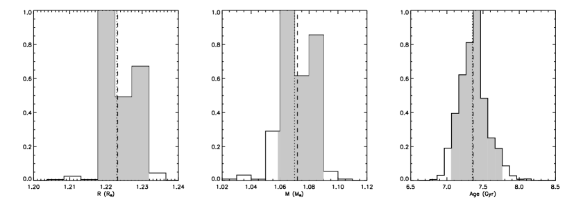
where $\chi^{2}$ is calculated from Eq. (3). By assuming flat priors on each of the model parameters, we then construct posterior probability functions (PPF) for each of the stellar properties to obtain more reliable estimates of the values and uncertainties from the dense ensemble of models sampled by the GA. We adopt the median value of the PPF as the best estimate for the parameter value, $\langle P\rangle$. We use the 68% credible interval of the PPF to define the associated uncertainty, $\sigma$. Sample PPFs for the radius, mass, and age of KIC 12069424 are shown in Fig. 1.

Combining the best estimates for each of the stellar properties generally will not produce the best stellar model. For many purposes it is useful to identify a reference model, an individual stellar model that is representative of the PPF. The optimal model identified by AMP, $P_{\rm AMP}$, is used as the reference model, but it can sometimes fall near the edge of one or more of the distributions. A comparison of the masses and ages estimated from $\langle P\rangle$ and $P_{\rm AMP}$ yields differences much smaller than 1$\sigma$ for most cases.

3.3 Validation with solar data

To validate our new approach, we used AMP 1.3 to match a set of solar oscillation frequencies comparable to the Kepler observations of 16 Cyg A and B (Metcalfe et al. 2015). The frequencies were derived from observations obtained with the Variability of solar IRradiance and Gravity Oscillations (VIRGO) instrument (Fröhlich et al. 1995) using 2.5 years of data (Davies et al. 2015). The best models identified by the four independent runs of the GA are listed in Table 2 under the headings AMP_N along with their individual $\chi^{2}$ values. The model with the lowest value of $\chi^{2}$ is the optimal solution identified by AMP, and this is adopted as the reference model. The remaining models reveal intrinsic parameter correlations, in particular between the mass and initial composition. The final two columns of Table 2 show the values of $\langle P\rangle$ and $\sigma$ derived from the PPFs, showing excellent agreement with the known solar properties: $R,M,L\equiv 1$, age $=4.60\pm 0.04$ Gyr (Houdek & Gough 2011).

Figure 4: Comparison of measured radii (top), luminosities (middle), and parallaxes (lower) with those deduced from the asteroseismic parameters. The interferometric radii are denoted by the red circles in the top panel, and the green triangle is the value from Masana et al. (2006)

4 Results

Table 3: Reference models of the Kepler targets and the Sun

KIC ID	$R$	$M$	Age	$Z_{i}$	$Y_{i}$	$\alpha$	$X_{c}/X_{i}$	$a_{0}$	$\chi^{2}_{N,r01}$	$\chi^{2}_{N,r02}$	$\chi^{2}_{N,\rm spec}$
	(R⊙)	(M⊙)	(Gyr)
Sun	1.003	1.01	4.38	0.0210	0.281	2.24	0.50	-2.54	1.03	0.78	0.71
1435467	1.704	1.41	1.87	0.0231	0.284	1.84	0.43	-3.95	2.68	1.64	1.49
2837475	1.613	1.41	1.70	0.0168	0.247	1.70	0.53	-4.48	1.29	2.07	0.32
3427720	1.125	1.13	2.17	0.0168	0.259	2.10	0.64	-2.41	1.10	1.26	0.15
3656476	1.326	1.10	8.48	0.0231	0.248	2.30	0.00	-2.22	2.35	0.68	1.57
3735871	1.089	1.08	1.57	0.0157	0.292	2.02	0.71	-3.64	1.47	0.67	0.05
4914923	1.326	1.01	7.15	0.0121	0.260	1.68	0.02	-4.51	0.56	1.50	3.35
5184732	1.365	1.27	4.70	0.0340	0.242	1.92	0.27	-4.43	6.98	2.32	0.85
5950854	1.257	1.01	9.01	0.0147	0.249	2.16	0.00	-1.27	0.60	4.61	1.30
6106415	1.213	1.06	4.43	0.0184	0.295	2.04	0.18	-3.48	0.93	2.81	0.54
6116048	1.239	1.06	5.84	0.0114	0.242	2.16	0.11	-3.27	3.27	2.48	0.44
6225718	1.194	1.06	2.30	0.0117	0.286	2.02	0.49	-5.99	3.47	0.97	0.64
6603624	1.159	1.03	8.64	0.0455	0.313	2.12	0.01	-2.34	3.42	135.14	5.90
6933899	1.535	1.03	6.58	0.0152	0.296	1.76	0.00	-4.38	1.45	1.25	0.21
7103006	1.957	1.56	1.94	0.0224	0.239	1.66	0.36	-7.28	1.15	0.69	1.33
7106245	1.120	0.97	6.05	0.0070	0.242	1.98	0.22	-4.02	2.96	0.73	4.41
7206837	1.579	1.41	1.72	0.0255	0.249	1.52	0.60	-4.61	1.48	1.43	1.52
7296438	1.371	1.10	5.93	0.0309	0.315	2.04	0.02	-2.76	0.74	0.53	0.47
7510397	1.828	1.30	3.58	0.0129	0.248	1.84	0.08	-2.37	0.75	2.23	0.55
7680114	1.395	1.07	7.04	0.0197	0.277	2.02	0.00	-3.00	1.63	0.74	0.00
7771282	1.645	1.30	3.13	0.0168	0.257	1.78	0.19	-4.03	2.10	0.75	0.33
7871531	0.859	0.80	9.32	0.0125	0.296	2.02	0.34	-4.15	1.06	0.65	1.25
7940546	1.917	1.39	2.58	0.0152	0.259	1.74	0.07	-6.26	2.47	0.82	1.45
7970740	0.779	0.78	10.59	0.0094	0.244	2.36	0.45	-2.55	4.93	5.09	3.34
8006161	0.954	1.06	4.34	0.0485	0.288	2.66	0.61	-0.63	2.33	1.21	1.26
8150065	1.394	1.20	3.33	0.0162	0.252	1.62	0.21	-3.97	2.03	2.30	0.66
8179536	1.353	1.26	2.03	0.0157	0.249	1.88	0.50	-3.89	1.51	0.62	0.01
8379927	1.105	1.08	1.65	0.0162	0.287	1.82	0.71	-4.98	1.87	1.63	0.33
8394589	1.169	1.06	3.82	0.0094	0.247	1.98	0.37	-3.14	0.71	0.70	0.01
8424992	1.056	0.94	9.62	0.0162	0.264	2.30	0.14	-1.38	0.70	0.30	0.22
8694723	1.493	1.04	4.22	0.0085	0.309	2.36	0.00	-2.23	0.70	1.46	3.18
8760414	1.028	0.82	12.09	0.0042	0.239	2.14	0.07	-2.42	0.52	1.69	4.43
8938364	1.361	1.00	11.00	0.0217	0.272	2.14	0.00	-2.09	1.44	3.52	3.26
9025370	1.000	0.97	5.50	0.0184	0.253	1.60	0.54	-6.01	1.45	3.78	0.27
9098294	1.151	0.99	8.22	0.0129	0.245	2.14	0.11	-3.13	1.93	0.96	0.23
9139151	1.167	1.20	1.84	0.0203	0.265	2.48	0.63	-1.58	1.66	1.26	0.17
9139163	1.582	1.49	1.26	0.0330	0.245	1.64	0.71	-9.60	0.95	1.89	4.25
9206432	1.499	1.37	1.32	0.0247	0.285	1.82	0.65	-2.37	1.68	1.10	0.72
9353712	2.183	1.56	2.17	0.0203	0.249	1.76	0.08	-1.89	2.57	0.73	1.16
9410862	1.159	0.99	6.15	0.0091	0.247	1.90	0.20	-3.11	1.28	0.75	0.74
9414417	1.896	1.40	2.67	0.0147	0.244	1.70	0.11	-5.41	1.01	0.78	0.39
9955598	0.876	0.87	6.38	0.0203	0.308	2.16	0.48	-2.71	1.15	2.13	0.13
9965715	1.224	0.99	3.00	0.0080	0.310	1.58	0.33	-5.57	0.78	0.65	1.76
10079226	1.135	1.09	2.35	0.0203	0.291	1.84	0.61	-4.10	1.39	0.73	0.12
10454113	1.282	1.27	2.03	0.0217	0.244	2.02	0.58	-0.79	2.07	4.38	1.79
10516096	1.407	1.08	6.44	0.0168	0.270	2.04	0.00	-2.81	1.29	1.14	0.65
10644253	1.073	1.04	1.14	0.0162	0.319	1.78	0.78	-4.91	0.78	0.62	0.31
10730618	1.729	1.33	2.55	0.0147	0.253	1.34	0.30	-2.14	2.04	3.36	0.14
10963065	1.210	1.04	4.28	0.0114	0.277	2.04	0.22	-3.53	1.41	0.98	0.00
11081729	1.393	1.25	1.88	0.0143	0.271	1.86	0.51	-5.62	6.03	5.17	1.56
11253226	1.635	1.53	1.06	0.0224	0.248	1.90	0.69	-4.76	2.76	1.83	2.00
11772920	0.839	0.81	11.11	0.0143	0.254	1.82	0.43	-3.90	2.28	0.35	0.33
12009504	1.379	1.13	3.44	0.0157	0.294	1.96	0.26	-4.67	0.81	0.88	0.10
12069127	2.262	1.58	1.89	0.0203	0.262	1.64	0.12	-4.46	3.00	0.79	0.02
12069424	1.223	1.07	7.35	0.0179	0.241	2.12	0.09	-4.41	3.78	1.02	1.39
12069449	1.105	1.01	6.88	0.0217	0.278	2.14	0.22	-2.90	4.93	0.94	0.69
12258514	1.601	1.25	6.11	0.0247	0.229	1.64	0.00	-4.04	2.45	0.92	9.89
12317678	1.749	1.27	2.18	0.0107	0.302	1.74	0.13	-5.26	1.22	1.09	0.65

Notes: The parameters are radius, mass, age, initial metallicity $Z_{i}$ and helium $Y_{i}$ mass fraction, mixing-length parameter $\alpha$, ratio of current central hydrogen to initial hydrogen mass fraction, $X_{c}/X_{i}$, the $a_{0}$ parameter in Eq. 7, and the normalized $\chi^{2}$ values for the $r_{01}$, $r_{02}$ and spectroscopic data.

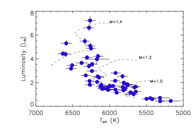
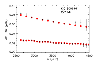
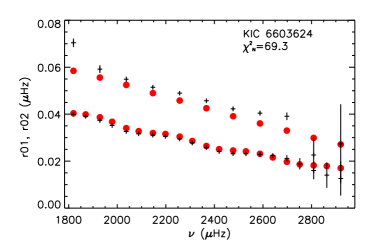
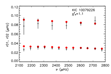
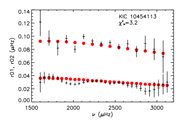
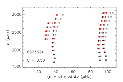
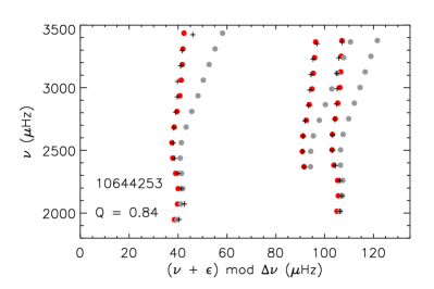
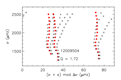
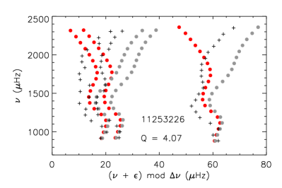
The sample of stars analyzed in this work span the main-sequence and early subgiant phase, as illustrated by their position in the Hertzsprung-Russell diagram (Fig. 2). They cover a range in mass of about 0.6 M_⊙, with about half of the sample being within 10% of the solar value. For a representative set of four stars, Fig. 3 compares the measured frequency separation ratios (crosses) with the corresponding values from the reference models (red filled dots). Here it can be seen that the agreement with the seismic observations is in general excellent, but some of the models do not necessarily reproduce features of the observed data. One example is KIC 10454113, which is shown in the lower right panel. It displays an oscillation as a function of frequency that the models fail to reproduce. These discrepancies are indeed noted in the normalized $\chi^{2}$ value, $\chi^{2}_{N}=\chi^{2}/N=3.2$, where $N$ is the number of frequency ratios. For KIC 8006161, shown in the top left panel, the fit is of higher quality with $\chi^{2}_{N}=1.8$. The parameters of the reference models that are used to compare with the observations are listed in Table 3 along with the individual $\chi^{2}_{N}$ values for $r_{01}$, $r_{02}$, and combined $T_{\rm eff}$ and [M/H].

For the Sun and each star in our sample, we derived a best estimate and uncertainty for the stellar radius, mass, age, metallicity, luminosity, and surface gravity using the method described in Sec. 3 (see Table 4). Using the rotation periods given in Table 1 and the derived radius, we also computed their rotational velocities.

Since the AMP 1.3 method uses only one set of physics in the stellar modeling, the derived uncertainties do not include possible systematic errors arising from errors in the model physics, such as the equation of state, heavy element settling, and convective overshoot. However, the uncertainties include sources of errors arising from free parameters that are often fixed in the stellar codes used in other methods, for example, the mixing-length parameter $\alpha$, the initial chemical composition $(X_{i},Y_{i},Z_{i}),$ or a chemical enrichment law. The uncertainty on these parameters contributes substantially to the error budget, and in some cases more so, for example, changing the equation of state or the opacities. The effect of such changes in the physics has been studied in detail for HD 52265 by Lebreton & Goupil (2014). A similar detailed analysis for each star in the sample we studied is beyond the scope of this paper. We refer to Silva Aguirre et al. (2017), who also analyzed data from Lund et al. (2017) using seven distinct modeling methods and codes.

The accuracy, namely the bias and not the precision, of our results can be ascertained by an analysis of the solar observations. As stated above, we derived a best-matched model with values for the mass of a 1 M_⊙ model and a radius of 1 R_⊙, and an age that, within the derived uncertainty, matches the solar value. A second accuracy test, at least for the age, can be established based on the independently derived ages for the binary system 16 Cyg A and B (also known as KIC 12069449 and KIC 12069424). The ages that we derive agree to within 1$\sigma$.

Table 4: Derived stellar properties of the Kepler targets and the Sun using VIRGO data

KIC ID	$R$	$M$	Age	$L$	$T_{\rm eff}$	$\log g$	[M/H]	$\pi$	$v$
	(R⊙)	(M⊙)	(Gyr)	(L⊙)	(K)	(dex)	(dex)	(mas)	(km s-1)
Sun	1.001 $\pm$ 0.005	1.001 $\pm$ 0.019	4.38 $\pm$ 0.22	0.97 $\pm$ 0.03	5732 $\pm$ 43	4.438 $\pm$ 0.003	0.07 $\pm$ 0.04
1435467	1.728 $\pm$ 0.027	1.466 $\pm$ 0.060	1.97 $\pm$ 0.17	4.29 $\pm$ 0.25	6299 $\pm$ 75	4.128 $\pm$ 0.004	0.09 $\pm$ 0.09	6.99 $\pm$ 0.24	13.09 $\pm$ 1.76
2837475	1.629 $\pm$ 0.027	1.460 $\pm$ 0.062	1.49 $\pm$ 0.22	4.54 $\pm$ 0.26	6600 $\pm$ 71	4.174 $\pm$ 0.007	0.05 $\pm$ 0.07	8.18 $\pm$ 0.29	22.40 $\pm$ 2.22
3427720	1.089 $\pm$ 0.009	1.034 $\pm$ 0.015	2.37 $\pm$ 0.23	1.37 $\pm$ 0.08	5989 $\pm$ 71	4.378 $\pm$ 0.003	-0.05 $\pm$ 0.09	11.04 $\pm$ 0.40	3.95 $\pm$ 0.61
3656476	1.322 $\pm$ 0.007	1.101 $\pm$ 0.025	8.88 $\pm$ 0.41	1.63 $\pm$ 0.06	5690 $\pm$ 53	4.235 $\pm$ 0.004	0.17 $\pm$ 0.07	8.49 $\pm$ 0.30	2.11 $\pm$ 0.24
3735871	1.080 $\pm$ 0.012	1.068 $\pm$ 0.035	1.55 $\pm$ 0.18	1.45 $\pm$ 0.09	6092 $\pm$ 75	4.395 $\pm$ 0.005	-0.05 $\pm$ 0.04	8.05 $\pm$ 0.31	4.74 $\pm$ 0.51
4914923	1.339 $\pm$ 0.015	1.039 $\pm$ 0.028	7.04 $\pm$ 0.50	1.79 $\pm$ 0.12	5769 $\pm$ 86	4.198 $\pm$ 0.004	-0.06 $\pm$ 0.09	8.64 $\pm$ 0.35	3.31 $\pm$ 0.46
5184732	1.354 $\pm$ 0.028	1.247 $\pm$ 0.071	4.32 $\pm$ 0.85	1.79 $\pm$ 0.15	5752 $\pm$ 101	4.268 $\pm$ 0.009	0.31 $\pm$ 0.06	14.53 $\pm$ 0.67	3.46 $\pm$ 0.43
5950854	1.254 $\pm$ 0.012	1.005 $\pm$ 0.035	9.25 $\pm$ 0.68	1.58 $\pm$ 0.11	5780 $\pm$ 74	4.245 $\pm$ 0.006	-0.11 $\pm$ 0.06	4.41 $\pm$ 0.18
6106415	1.205 $\pm$ 0.009	1.039 $\pm$ 0.021	4.55 $\pm$ 0.28	1.61 $\pm$ 0.09	5927 $\pm$ 63	4.294 $\pm$ 0.003	-0.00 $\pm$ 0.04	25.35 $\pm$ 0.87
6116048	1.233 $\pm$ 0.011	1.048 $\pm$ 0.028	6.08 $\pm$ 0.40	1.77 $\pm$ 0.13	5993 $\pm$ 73	4.276 $\pm$ 0.003	-0.20 $\pm$ 0.08	13.31 $\pm$ 0.57	3.61 $\pm$ 0.41
6225718	1.234 $\pm$ 0.018	1.169 $\pm$ 0.039	2.23 $\pm$ 0.20	2.08 $\pm$ 0.11	6252 $\pm$ 63	4.321 $\pm$ 0.005	-0.09 $\pm$ 0.06	19.32 $\pm$ 0.60
6603624	1.164 $\pm$ 0.024	1.058 $\pm$ 0.075	8.66 $\pm$ 0.68	1.23 $\pm$ 0.11	5644 $\pm$ 91	4.326 $\pm$ 0.008	0.24 $\pm$ 0.05	11.89 $\pm$ 0.59
6933899	1.597 $\pm$ 0.008	1.155 $\pm$ 0.011	7.22 $\pm$ 0.53	2.63 $\pm$ 0.06	5815 $\pm$ 47	4.093 $\pm$ 0.002	0.11 $\pm$ 0.03	6.48 $\pm$ 0.15
7103006	1.958 $\pm$ 0.025	1.568 $\pm$ 0.051	1.69 $\pm$ 0.12	5.58 $\pm$ 0.36	6332 $\pm$ 89	4.048 $\pm$ 0.006	0.09 $\pm$ 0.10	6.19 $\pm$ 0.23	21.44 $\pm$ 2.25
7106245	1.125 $\pm$ 0.009	0.989 $\pm$ 0.023	6.05 $\pm$ 0.39	1.56 $\pm$ 0.09	6078 $\pm$ 74	4.327 $\pm$ 0.003	-0.44 $\pm$ 0.11	4.98 $\pm$ 0.20
7206837	1.556 $\pm$ 0.018	1.377 $\pm$ 0.039	1.55 $\pm$ 0.50	3.37 $\pm$ 0.15	6269 $\pm$ 87	4.191 $\pm$ 0.008	0.07 $\pm$ 0.15	5.28 $\pm$ 0.15	19.49 $\pm$ 1.37
7296438	1.370 $\pm$ 0.009	1.099 $\pm$ 0.022	6.37 $\pm$ 0.60	1.85 $\pm$ 0.08	5754 $\pm$ 55	4.205 $\pm$ 0.003	0.21 $\pm$ 0.07	6.09 $\pm$ 0.18	2.76 $\pm$ 0.30
7510397	1.823 $\pm$ 0.018	1.309 $\pm$ 0.037	3.51 $\pm$ 0.24	4.19 $\pm$ 0.20	6119 $\pm$ 69	4.031 $\pm$ 0.004	-0.14 $\pm$ 0.06	11.75 $\pm$ 0.36
7680114	1.402 $\pm$ 0.014	1.092 $\pm$ 0.030	6.89 $\pm$ 0.46	2.07 $\pm$ 0.09	5833 $\pm$ 47	4.181 $\pm$ 0.004	0.08 $\pm$ 0.07	5.73 $\pm$ 0.17	2.70 $\pm$ 0.19
7771282	1.629 $\pm$ 0.016	1.268 $\pm$ 0.040	2.78 $\pm$ 0.47	3.61 $\pm$ 0.18	6223 $\pm$ 73	4.118 $\pm$ 0.004	-0.03 $\pm$ 0.07	3.24 $\pm$ 0.10	6.94 $\pm$ 0.54
7871531	0.871 $\pm$ 0.008	0.834 $\pm$ 0.021	8.84 $\pm$ 0.46	0.60 $\pm$ 0.05	5482 $\pm$ 69	4.478 $\pm$ 0.006	-0.16 $\pm$ 0.04	16.81 $\pm$ 0.81	1.31 $\pm$ 0.10
7940546	1.974 $\pm$ 0.045	1.511 $\pm$ 0.087	2.42 $\pm$ 0.17	5.69 $\pm$ 0.35	6330 $\pm$ 43	4.023 $\pm$ 0.005	0.00 $\pm$ 0.06	12.16 $\pm$ 0.44	8.79 $\pm$ 0.76
7970740	0.776 $\pm$ 0.007	0.768 $\pm$ 0.019	10.53 $\pm$ 0.43	0.42 $\pm$ 0.04	5282 $\pm$ 93	4.546 $\pm$ 0.003	-0.37 $\pm$ 0.09	36.83 $\pm$ 1.71	2.19 $\pm$ 0.38
8006161	0.930 $\pm$ 0.009	1.000 $\pm$ 0.030	4.57 $\pm$ 0.36	0.64 $\pm$ 0.03	5351 $\pm$ 49	4.498 $\pm$ 0.003	0.41 $\pm$ 0.04	37.89 $\pm$ 1.18	1.58 $\pm$ 0.16
8150065	1.402 $\pm$ 0.018	1.222 $\pm$ 0.040	3.15 $\pm$ 0.49	2.52 $\pm$ 0.19	6138 $\pm$ 105	4.230 $\pm$ 0.005	-0.04 $\pm$ 0.15	3.94 $\pm$ 0.18
8179536	1.350 $\pm$ 0.013	1.249 $\pm$ 0.031	1.88 $\pm$ 0.25	2.63 $\pm$ 0.11	6318 $\pm$ 59	4.274 $\pm$ 0.005	-0.04 $\pm$ 0.07	6.91 $\pm$ 0.20	2.78 $\pm$ 0.18
8379927	1.102 $\pm$ 0.012	1.073 $\pm$ 0.033	1.64 $\pm$ 0.12	1.39 $\pm$ 0.10	5971 $\pm$ 91	4.382 $\pm$ 0.005	-0.04 $\pm$ 0.05	30.15 $\pm$ 1.40	3.28 $\pm$ 0.26
8394589	1.155 $\pm$ 0.009	1.024 $\pm$ 0.030	3.82 $\pm$ 0.25	1.68 $\pm$ 0.09	6103 $\pm$ 61	4.324 $\pm$ 0.003	-0.28 $\pm$ 0.07	8.47 $\pm$ 0.28
8424992	1.048 $\pm$ 0.005	0.930 $\pm$ 0.016	9.79 $\pm$ 0.76	0.99 $\pm$ 0.04	5634 $\pm$ 57	4.362 $\pm$ 0.002	-0.12 $\pm$ 0.06	7.52 $\pm$ 0.23
8694723	1.463 $\pm$ 0.023	1.004 $\pm$ 0.036	4.85 $\pm$ 0.22	3.15 $\pm$ 0.18	6347 $\pm$ 67	4.107 $\pm$ 0.004	-0.38 $\pm$ 0.08	8.18 $\pm$ 0.28
8760414	1.027 $\pm$ 0.004	0.814 $\pm$ 0.011	11.88 $\pm$ 0.34	1.15 $\pm$ 0.06	5915 $\pm$ 54	4.329 $\pm$ 0.002	-0.66 $\pm$ 0.07	9.83 $\pm$ 0.32
8938364	1.362 $\pm$ 0.007	1.015 $\pm$ 0.023	10.85 $\pm$ 1.22	1.65 $\pm$ 0.15	5604 $\pm$ 115	4.174 $\pm$ 0.004	0.06 $\pm$ 0.06	6.27 $\pm$ 0.31
9025370	0.997 $\pm$ 0.017	0.969 $\pm$ 0.036	5.53 $\pm$ 0.43	0.71 $\pm$ 0.11	5296 $\pm$ 157	4.424 $\pm$ 0.006	0.01 $\pm$ 0.09	15.66 $\pm$ 1.44
9098294	1.150 $\pm$ 0.003	0.979 $\pm$ 0.017	8.23 $\pm$ 0.53	1.34 $\pm$ 0.05	5795 $\pm$ 53	4.312 $\pm$ 0.002	-0.17 $\pm$ 0.07	8.30 $\pm$ 0.23	2.94 $\pm$ 0.20
9139151	1.137 $\pm$ 0.027	1.129 $\pm$ 0.091	1.94 $\pm$ 0.31	1.81 $\pm$ 0.11	6270 $\pm$ 63	4.375 $\pm$ 0.008	0.05 $\pm$ 0.10	9.57 $\pm$ 0.34	5.25 $\pm$ 1.07
9139163	1.569 $\pm$ 0.027	1.480 $\pm$ 0.085	1.23 $\pm$ 0.15	3.51 $\pm$ 0.24	6318 $\pm$ 105	4.213 $\pm$ 0.004	0.11 $\pm$ 0.00	9.85 $\pm$ 0.39
9206432	1.460 $\pm$ 0.015	1.301 $\pm$ 0.048	1.48 $\pm$ 0.31	3.47 $\pm$ 0.18	6508 $\pm$ 75	4.219 $\pm$ 0.009	0.06 $\pm$ 0.07	7.03 $\pm$ 0.26	8.39 $\pm$ 1.01
9353712	2.240 $\pm$ 0.061	1.681 $\pm$ 0.125	1.91 $\pm$ 0.14	7.27 $\pm$ 1.02	6343 $\pm$ 119	3.965 $\pm$ 0.008	0.12 $\pm$ 0.08	2.21 $\pm$ 0.16	10.03 $\pm$ 1.03
9410862	1.149 $\pm$ 0.009	0.969 $\pm$ 0.017	5.78 $\pm$ 0.82	1.56 $\pm$ 0.08	6017 $\pm$ 69	4.304 $\pm$ 0.003	-0.34 $\pm$ 0.08	5.05 $\pm$ 0.16	2.55 $\pm$ 0.27
9414417	1.891 $\pm$ 0.015	1.401 $\pm$ 0.028	2.53 $\pm$ 0.17	4.98 $\pm$ 0.22	6260 $\pm$ 67	4.028 $\pm$ 0.004	-0.07 $\pm$ 0.12	4.65 $\pm$ 0.13	8.96 $\pm$ 0.56
9955598	0.881 $\pm$ 0.008	0.885 $\pm$ 0.023	6.47 $\pm$ 0.45	0.58 $\pm$ 0.03	5400 $\pm$ 57	4.494 $\pm$ 0.003	0.06 $\pm$ 0.04	14.98 $\pm$ 0.53	1.30 $\pm$ 0.22
9965715	1.234 $\pm$ 0.015	1.005 $\pm$ 0.033	3.29 $\pm$ 0.33	1.85 $\pm$ 0.15	6058 $\pm$ 113	4.258 $\pm$ 0.004	-0.27 $\pm$ 0.11	8.81 $\pm$ 0.51
10079226	1.129 $\pm$ 0.016	1.082 $\pm$ 0.048	2.75 $\pm$ 0.42	1.41 $\pm$ 0.10	5915 $\pm$ 89	4.364 $\pm$ 0.005	0.07 $\pm$ 0.06	7.05 $\pm$ 0.29	3.86 $\pm$ 0.33
10454113	1.272 $\pm$ 0.006	1.260 $\pm$ 0.016	2.06 $\pm$ 0.16	2.07 $\pm$ 0.08	6134 $\pm$ 61	4.325 $\pm$ 0.003	0.04 $\pm$ 0.04	11.94 $\pm$ 0.63	4.41 $\pm$ 0.33
10516096	1.398 $\pm$ 0.008	1.065 $\pm$ 0.012	6.59 $\pm$ 0.37	2.11 $\pm$ 0.08	5872 $\pm$ 43	4.173 $\pm$ 0.003	-0.06 $\pm$ 0.06	7.53 $\pm$ 0.21
10644253	1.090 $\pm$ 0.027	1.091 $\pm$ 0.097	0.94 $\pm$ 0.26	1.45 $\pm$ 0.09	6033 $\pm$ 67	4.399 $\pm$ 0.007	0.01 $\pm$ 0.10	10.45 $\pm$ 0.39	5.05 $\pm$ 0.42
10730618	1.763 $\pm$ 0.040	1.411 $\pm$ 0.097	1.81 $\pm$ 0.41	4.04 $\pm$ 0.56	6156 $\pm$ 181	4.095 $\pm$ 0.011	0.05 $\pm$ 0.18	3.35 $\pm$ 0.27
10963065	1.204 $\pm$ 0.007	1.023 $\pm$ 0.024	4.33 $\pm$ 0.30	1.80 $\pm$ 0.08	6097 $\pm$ 53	4.288 $\pm$ 0.003	-0.24 $\pm$ 0.06	11.46 $\pm$ 0.34	4.84 $\pm$ 0.65
11081729	1.423 $\pm$ 0.009	1.257 $\pm$ 0.045	2.22 $\pm$ 0.10	3.29 $\pm$ 0.07	6474 $\pm$ 43	4.215 $\pm$ 0.026	0.07 $\pm$ 0.03	7.48 $\pm$ 0.17	26.28 $\pm$ 2.98
11253226	1.606 $\pm$ 0.015	1.486 $\pm$ 0.030	0.97 $\pm$ 0.21	4.80 $\pm$ 0.20	6696 $\pm$ 79	4.197 $\pm$ 0.007	0.10 $\pm$ 0.05	8.07 $\pm$ 0.23	22.32 $\pm$ 2.28
11772920	0.845 $\pm$ 0.009	0.830 $\pm$ 0.028	10.79 $\pm$ 0.96	0.42 $\pm$ 0.06	5084 $\pm$ 159	4.502 $\pm$ 0.004	-0.06 $\pm$ 0.09	14.82 $\pm$ 1.24
12009504	1.382 $\pm$ 0.022	1.137 $\pm$ 0.063	3.44 $\pm$ 0.44	2.46 $\pm$ 0.25	6140 $\pm$ 133	4.213 $\pm$ 0.006	-0.04 $\pm$ 0.05	7.51 $\pm$ 0.42	7.44 $\pm$ 0.55
12069127	2.283 $\pm$ 0.033	1.621 $\pm$ 0.084	1.79 $\pm$ 0.14	7.26 $\pm$ 0.42	6267 $\pm$ 79	3.926 $\pm$ 0.010	0.15 $\pm$ 0.08	2.35 $\pm$ 0.08	125.54 $\pm$ 7.07
12069424	1.223 $\pm$ 0.005	1.072 $\pm$ 0.013	7.36 $\pm$ 0.31	1.52 $\pm$ 0.05	5785 $\pm$ 39	4.294 $\pm$ 0.001	-0.04 $\pm$ 0.05	47.44 $\pm$ 1.00	2.60 $\pm$ 0.20
12069449	1.113 $\pm$ 0.016	1.038 $\pm$ 0.047	7.05 $\pm$ 0.63	1.21 $\pm$ 0.11	5732 $\pm$ 83	4.361 $\pm$ 0.007	0.15 $\pm$ 0.08	46.77 $\pm$ 2.10	2.43 $\pm$ 0.63
12258514	1.593 $\pm$ 0.016	1.251 $\pm$ 0.016	5.50 $\pm$ 0.40	2.63 $\pm$ 0.12	5808 $\pm$ 61	4.129 $\pm$ 0.002	0.10 $\pm$ 0.09	12.79 $\pm$ 0.40	5.37 $\pm$ 0.66
12317678	1.788 $\pm$ 0.014	1.373 $\pm$ 0.030	2.30 $\pm$ 0.20	5.49 $\pm$ 0.28	6587 $\pm$ 97	4.064 $\pm$ 0.005	-0.26 $\pm$ 0.09	6.89 $\pm$ 0.23

Notes: The mean model parameters are radius, mass, age, luminosity, effective temperature, surface gravity, metallicity, parallax, and rotational velocity. The latter two are derived using data from this table and Table 1.

4.1 Accuracy of radii and luminosities

To test the accuracy of the derived radii and luminosities, we have compiled measured values of these properties for nine stars (Table 5). These stars have reliable Hipparcos parallaxes and are not members of close binary systems. Only three of the radii of the subsample of stars have been measured interferometrically (Huber et al. 2012; White et al. 2013). The angular diameters from Masana et al. (2006) and Huber et al. (2014) were derived from broadband photometry and from literature atmospheric properties and stellar evolution models, respectively. Metcalfe et al. (2012) and Metcalfe et al. (2014) derived the luminosities using extinction estimates from Ammons et al. (2006) and the bolometric corrections from Flower (1996, see Torres 2010).

Table 5: Luminosities, radii, and parallaxes from independent sources

KIC ID	$L$	$R$	$\pi$
	(L⊙)	(R⊙)	(mas)
8006161	0.61 $\pm$ 0.02	0.9501 $\pm$ 0.020	37.47 $\pm$ 0.49
9139151	1.63 $\pm$ 0.40	1.1603 $\pm$ 0.020	9.46 $\pm$ 1.15
9139163	3.88 $\pm$ 0.69	1.5703 $\pm$ 0.030	9.49 $\pm$ 0.83
9206432	4.95 $\pm$ 1.48	1.5203 $\pm$ 0.030	5.85 $\pm$ 0.87
10454113	2.60 $\pm$ 0.36	1.2403 $\pm$ 0.020	9.95 $\pm$ 0.67
11253226	4.22 $\pm$ 0.61	1.5764 $\pm$ 0.143	8.52 $\pm$ 0.60
12069424	1.56 $\pm$ 0.05	1.2201 $\pm$ 0.020	47.44 $\pm$ 0.27
12069449	1.27 $\pm$ 0.04	1.1201 $\pm$ 0.020	47.14 $\pm$ 0.27
12258514	2.84 $\pm$ 0.25	1.5903 $\pm$ 0.040	12.32 $\pm$ 0.51

The luminosities are from Metcalfe et al. (2012, 2014). The references to the radii are ¹Huber et al. (2012) ²White et al. (2013) ³Huber et al. (2014) ⁴Masana et al. (2006). The parallaxes are from van Leeuwen (2007).

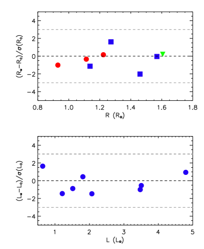
A comparison of these independent measures of stellar radii and luminosities with those derived using our asteroseismic methodology is shown in the top two panels of Fig. 4. This comparison, using measurement differences relative to their uncertainty as listed in the literature, shows no systematic biases or trends for this subsample of nine stars. The mean relative difference is –0.40 with a root mean square (rms) around the mean of 0.59 for the interferometrically measured radii (references 1 and 2, red filled circles) and –0.28 $\pm$ 1.03 for the radii derived using photometry and isochrones (references 3 and 4). For the luminosity the mean relative difference is –0.35 with an rms around the mean of 1.1.

4.2 Asteroseismic parallaxes

We used the luminosity $L$ that was derived from the asteroseismic analysis to compute the stellar distance as a parallax. Using the modeled surface gravity and the observed $T_{\rm eff}$ and [M/H], we derived the amount of interstellar absorption between the top of the Earth’s atmosphere and the star, $A_{Ks}$, using the isochrone method described in Schultheis et al. (2014). Here, the subscript $Ks$ refers to the 2MASS $K_{s}$ filter (Skrutskie et al. 2006). With the same observed $T_{\rm eff}$ , we computed the corresponding bolometric correction $BC_{Ks}$ for this band, using $BC_{Ks}=4.51465-0.000524461T_{\rm eff}$ (Marigo et al. 2008) where the solar bolometric magnitude is 4.72 mag. The $K_{s}$-band magnitude and $A_{Ks}$ are listed in Table 1. The distance, $d$, or parallax, $\pi$, is then computed directly from $L$, $K_{s}$, $BC_{Ks}$ , and $A_{Ks}$.

The parallaxes and uncertainties of the stars in our sample are listed in Table 4. They were derived using Monte Carlo simulations, described as follows. We perturbed each of the input data measures $L$, $A_{Ks}$, $K_{s}$, and $BC_{K}$, using noise sampled from a Gaussian distribution with zero mean and standard deviation equivalent to their errors to calculate a parallax. By repeating the perturbations 10,000 times, we obtained a distribution of parallaxes, which is modeled by a Gaussian function. The mean and standard deviation are adopted as the parallax value and its uncertainty. In most cases, the derived parallax error is dominated by the luminosity error.

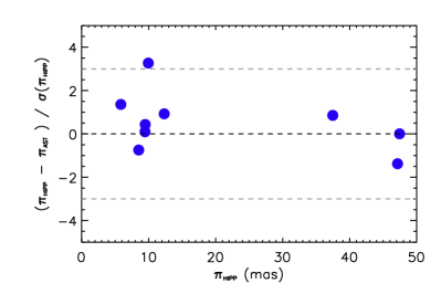
A comparison between the derived parallaxes and existing literature values (van Leeuwen 2007, Table 5) again validates our results, as shown in the lower panel of Fig. 4, where no significant trend can be seen. In particular, we note that for the binary KIC 12069424 and KIC 12069449 (16 Cyg A&B), we obtain almost identical parallaxes of 47.4 mas and 46.8 mas, equivalent to a difference of 0.3 pc at a distance of 21.2 pc. This result provides further evidence of the accuracy of our derived properties.

4.3 Trends in stellar properties

Performing a homogenous analysis on a relatively large sample allows us to check for trends in some stellar parameters and compare them to trends derived or established by other methods. We performed this check for two parameters: the mixing-length parameter and the stellar age.

4.3.1 Mixing-length parameter versus $T_{\rm eff}$ and $\log g$

The mixing-length parameter $\alpha$ is usually calibrated for a solar model and then applied to all models for a set range of masses and metallicities. However, several authors have shown that this approach is not correct, for instance, Yıldız et al. (2006); Bonaca et al. (2012); Creevey et al. (2012). The values of $\alpha$ resulting from a GA analysis offer an optimal approach to effectively test and subsequently constrain this parameter, since by design the GA only restricts $\alpha$ to be between 1.0 and 3.0, a range large enough to encompass all plausible values.

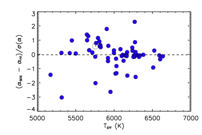
The color-coded distribution of $\alpha$ with $\log g$ and $T_{\rm eff}$ is shown in the top panel of Fig. 5, using the results derived from our sample of 57 stars and the Sun. It is evident from this figure that for a given value of $\log g$, the value of $\alpha$ has an upper limit. This upper limit can be represented by the equation $\alpha<1.65\log g-4.75$, and this is denoted by the dashed line in the figure. A regression analysis considering the model values of $\log g$, $\log$$T_{\rm eff}$ and [M/H] yields

$$\indent\alpha = 5.972778+0.636997\log g$$

$$-1.799968\log T_{\rm eff}+0.040094[{\rm M}/{\rm H}],$$

with a mean and rms of the residual to the fit of –0.01 $\pm$ 0.15 for the 58 stars. The residuals of this fit scaled by the uncertainties in $\alpha$ are shown in the lower panel of Fig. 5 as a function of $T_{\rm eff}$. No trend with this parameter can be seen. This equation yields a value of $\alpha=2.03$ for the known solar properties, within 1$\sigma$ of its mean value (2.12).

Figure 5: Top: Distribution of the $\log g$ and $\alpha$ for the full sample. The color coding shows in red $T_{\rm eff}$ $<$ 5600 K, in yellow 5600 K $<$ $T_{\rm eff}$ $<$ 6000 K, in green 6000 K $<$ $T_{\rm eff}$ $<$ 6300 K, and blue $T_{\rm eff}$ $>$ 6300 K. Bottom: Residuals of the regression analysis scaled by the uncertainties in $\alpha$ as a function of $T_{\rm eff}$.

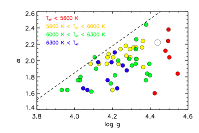
These results agree in part with those derived by Magic et al. (2015), who used a full 3D radiative hydrodynamic simulation for modeling convective envelopes. These authors found that $\alpha$ increases with $\log g$ and decreases with $T_{\rm eff}$, which is qualitatively in agreement with our results. The size of the variation that they inferred, however, is smaller than the values we find. In our sample, $\alpha$ varies between 1.7 and 2.4, while for the same range in $\log g$, $T_{\rm eff}$, Magic et al. see variations in $\alpha$ from 1.9 to 2.3. We note that the range of metallicity in our sample is much smaller than the range in their work. This could be the reason of the weak and opposite dependence on $\alpha$ that we find.

4.3.2 Age and $\langle r_{02}\rangle$

Figure 6: Age determination as a function of the mean value of $r02$.

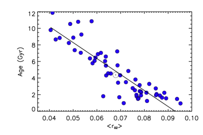
The $r_{02}$ frequency ratios contain what is known as small frequency separations, and these are effective at probing the gradients near the core of the star (Roxburgh & Vorontsov 2003). As the core is most sensitive to nuclear processing, $r_{02}$ are a diagnostic of the evolutionary state of the star. Using theoretical models, Lebreton & Montalbán (2009) showed a relationship between the mean value of $r_{02}$ and the stellar age. This relationship was recently used by Appourchaux et al. (2015) to estimate the age of the binary KIC 7510397 (HIP 93511).

Figure 6 shows the distribution of the mean of the $r_{02}$ ratios, that is, $\langle r_{02}\rangle$, versus the derived ages for the sample of stars studied here. A linear fit to these data leads to the following estimate of the stellar age, $\tau$ in Gyr, based on $\langle r_{02}\rangle$

$$\tau=17.910-193.918\langle r_{02}\rangle,$$ (6)

This is, of course, only valid for the range covered by our sample. The range of radial orders used for calculating $\langle r_{02}\rangle$ has almost no impact on this result (an effect lower than a 1%). We note that when inserting the value of $\langle r_{02}\rangle=0.068$ for the Sun, Eq. 6 yields an age of 4.7 Gyr, in excellent agreement with the Sun’s age as determined by other means.

5 Characterizing surface effects

It is known that a direct comparison of observed frequencies with model frequencies derived from 1D stellar structure models reveals a systematic discrepancy that increases with the mode frequency; this is commonly referred to as surface effects (Rosenthal 1997, see Section 1). This discrepancy arises because a 1D stellar atmosphere does not represent the actual structural and thermal properties of the stellar atmosphere in the layers close to the surface and because non-adiabatic effects that are present immediately below the surface are not included when computing resonant frequencies using an adiabatic code. Some recent works have attempted to produce more realistic stellar atmospheres by replacing the outer layers of a 1D stellar envelope by an averaged 3D surface simulation and by including the effects of turbulent pressure in the equation of hydrostatic support and opacity changes from the temperature fluctuations, and by also considering non-adiabatic effects (Trampedach et al. 2014, 2017; Houdek et al. 2016). This reduced the approximately $-$15 $\mu$Hz discrepancy to around +2 $\mu$Hz near 4,000 $\mu$Hz when including both structural and modal effects. While progress is being made, we are still not in a position to apply these calculations for a large sample of stars.

To sidestep this problem, several authors have suggested the use of combination frequencies that are insensitive to this systematic offset in frequency, see for example, Roxburgh & Vorontsov (2003), hence the exclusive use of $r_{01}$ and $r_{02}$ in the AMP 1.3 method. However, since individual frequencies contain more information than ratios of frequency separations, some authors have derived simple prescriptions to mitigate the surface effects. One such parametrization is that of Kjeldsen et al. (2008), who suggested a simple correction to the 1D model frequencies $\delta\nu_{n,l}$ of the form of a power law,

$$\delta\nu_{n,l}=a_{0}\left(\frac{\nu^{\rm obs}_{n,l}}{\nu_{\rm max}}\right)^{b},$$ (7)

where $b=4.82$ is a fixed value, calibrated by a solar model, $\nu_{\rm max}$ is the frequency corresponding to the highest amplitude mode, see (Lund et al. 2017), $a_{0}$ is computed from the differences between the observed and model frequencies (Metcalfe et al. 2009, 2014),

$$a_{0}=\frac{\langle\nu_{n,0}^{\rm obs}\rangle-\langle\nu_{n,0}^{\rm mod}\rangle}{N^{-1}_{0}\sum_{i=1}^{N_{0}}[\nu^{\rm obs}_{i}/\nu_{\rm max}]^{b}}.$$ (8)

$\text{Here, }\nu^{\rm obs}_{n,l}$ and $\nu^{\rm mod}_{n,l}$ are the observed and model frequency of radial order $n$ and degree $l$, respectively, and $N_{0}$ is the number of $l=0$ frequencies.

In the absence of perfect 3D simulations, the interest in using such a surface correction becomes evident when we consider not only that the individual frequencies contain a higher information content, but more importantly, that the $r_{01}$ and $r_{02}$ frequency ratios are only useful if the precision on these derived quantities is high enough. A precision like this on the ratio requires not only having a high precision on the individual frequencies, but enough radial order modes to constrain the stellar modeling. This is not necessarily the case for some stars, where, for example, ground-based campaigns are limited in time-domain coverage, such as the case of $\nu$ Ind (Carrier et al. 2007), or even for space-based missions such as the TESS mission, where only one month of continuous data will be available for stars at certain galactic latitudes. Similary, limited precision will also be achieved for the stars observed in the PLATO step-and-stare phase, since the observation window will only be two to three months each.

The AMP 1.3 method exclusively uses the $r_{01}$ and $r_{02}$ frequency ratios, and our results are therefore expected to be insensitive to surface effects. Hence, using the resulting models and the observed frequencies, we can explore the nature of the surface term for a large sample of stars, and in particular, we can test to which extent the Kjeldsen et al. (2008) prescription is useful.

5.1 Surface effects as observed in the Sun at low degrees

The magnitude of the surface effects on the frequency discrepancy for the Sun is on the order of 10-15 $\mu$Hz around 4000 $\mu$Hz for the low degrees ($l=0,1,2,\text{and }3$). Our analysis using the solar data reveals a similar offset. In the top panel of Fig. 7 we show the solar surface term by comparing the input frequencies with those of the models. The term of the reference model is shown by the thick line with filled black dots, and in gray we show those for 100 of the best solar models, with the mean of these 100 shown as the thick dashed line. At $\nu_{\rm max}$, the value of $a_{0}=-2.5\mu$Hz for the reference model, and for 100 of the representative models it spans –2.3 to –4.6 $\mu$Hz.

Figure 7: Top: Surface term for the reference solar model (connected black dots) for the $l=0$ frequencies as a function of observed frequency scaled by $\nu_{\rm max}$. The surface term for a sample of 100 of the best models is also shown for the Sun (gray), with the mean value highlighted by the dashed line. The blue connected squares show the empirical surface correction $\delta\nu_{n,l}$ (Eq. 7) based on the reference model. Lower: The differences between the observed and corrected model frequencies as a function of scaled frequency, with the solar observational errors overplotted in blue. The shaded gray areas represent the mean and standard deviation of $q$ for the same 100 models shown in the top panel. The dotted vertical lines delimit the region used to calculate the quality metric $Q$.

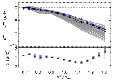
When we apply Eq. 7 to the reference solar model, we calculate a correction $\delta\nu_{n,l}$ that successfully mitigates the surface effects. This is clearly shown in the top panel of Fig. 7 , where the surface term for the reference model (black connected dots) is traced by the scaled surface correction $\delta\nu$ (blue connected squares) for the $l=0$ modes alone. By applying the proposed corrections $\delta\nu_{n,l}$ to the observed frequencies, we can then make a quantitive comparison between the model and the data. This agreement is shown in the lower panel for $l=0,$ and we denote it as $q_{n,l}=\nu^{\rm obs}_{n,l}-\nu^{\rm mod}_{n,l}+\delta\nu_{n,l}$. To quantify the agreement between the corrected model frequencies and the observed ones, we define the metric $Q$ as the median of the absolute value of the residuals,

$$\\ Q=\mathrm{median}\left|{q_{n,l}}\right|,$$ (9)

for all observed $n$ and $l$ defined in the region of $0.7\leq\nu_{n,l}^{\rm obs}/\nu_{\rm max}\leq 1.3$. This region is delimited in the lower panel by the vertical dotted lines. We note that we purposely exclude any reference to an observational error in the definition of $q$, as the surface correction results from an error in the models and is not related to the precision of the frequency data. In the ideal case and in the absence of errors in the data, $Q\rightarrow 0\leavevmode\nobreak\ \mu$Hz, which means that the model is perfect. The value of $Q$ is 0.38 $\mu$Hz for the reference solar model, and the mean value for the 100 solar models shown in Fig. 7 is 0.51 $\mu$Hz. From this figure and the low value of the quality metric, it is expected that the Kjeldsen et al. (2008) empirical surface correction $\delta\nu_{n,l}$ (Eq. 7) is useful for mitigating the surface effects for this solar model.

5.2 Surface effects for other stars

Is the simplified surface correction useful in other stars? And if so, to what extent? These are the questions that we aim to answer by inspecting the reference models (Table 3) of the best-fit stars within our sample.

We define a subset of stars by selecting those with $\chi^{2}_{N}\leq 3.0$ for both $r_{01}$ and $r_{02}$. This selection results in a subset of 44 stars. The differences between the observed frequencies and the frequencies of the reference models for this subset are shown in Fig. 8, and we assume that these differences are dominated by the surface effects. For the stars represented by the continuous lines it can be noted that the remaining discrepancies are quite similar in magnitude and shape for the less evolved stars. For the more evolved stars ($\log g$ $>$ 4.2, indicated by dashed lines), the remaining discrepancies are larger and of a different nature, and cannot readily be modeled by a simple power law.

Figure 8: Surface terms for the stars in our subsample defined by the criteria of $\chi_{N}^{2}(r_{01},r_{02})\leq 3$. For clarity, the more evolved stars are shown by the dashed lines.

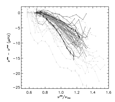
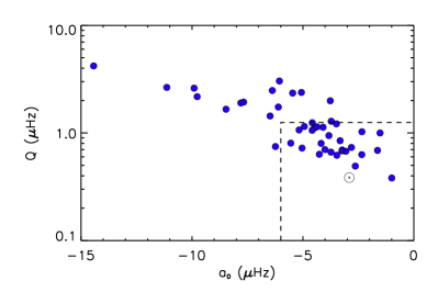
For each of the stars, a value of $a_{0}$ is derived directly from the comparison of model and observed frequencies (see Table 4), and Eq. 7 is used to calculate the surface correction $\delta\nu_{n,l}$ to apply to the model frequencies. We then calculate the metric $Q$ for each star in the subsample, and these values are shown as a function of $a_{0}$ in Fig. 9. We see very clearly that as the difference between the observed and model frequency at $\nu_{\rm max}$ increases (i.e., $a_{0}$ becomes more negative), $Q$ also increases, indicating that the Kjeldsen et al. (2008) correction becomes less adequate to mitigate the surface effects. It seems then quite likely that there is a value of $Q$ (and $a_{0}$) that defines a limit where the surface correction is useful.

By inspecting the residuals between observed and corrected model frequencies for this subset of stars, we found that when $Q\lesssim 1.0\leavevmode\nobreak\ \mu$Hz, we obtained a very good match to the observed frequencies when the surface correction was included. These stars also have values of $a_{0}$ that are typically lower than $-$6.0 $\mu$Hz, as shown in Fig. 9, just like the solar case. For an illustration, we present some échelle diagrams in Fig. 13 with different values of $Q$ to show the validity of this criterion. A visual inspection of the residuals and the échelle diagrams for this subsample of stars led to the same conclusion.

Figure 9: Metric $Q$ versus $a_{0}$ for the stars in our subsample. The dashed lines highlight the approximate limitation in $Q$ and $a_{0}$ where the surface correction enables a useful comparison between the observed and corrected model frequencies.

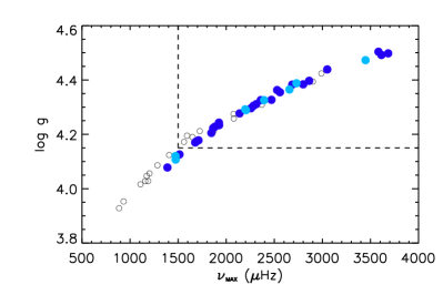
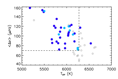
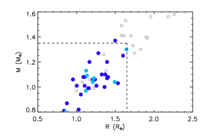
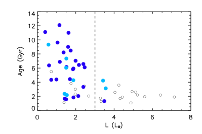
When we rely on the criteria of $Q\lesssim 1$ $\mu$Hz, we can trace the ranges of the stellar parameters where the surface correction mitigates the surface effects. This is presented in Fig. 10, which shows the distribution of observed and inferred stellar properties of stars from this subsample (open circles) along with the stars that satisfy the criterion of $Q\lesssim 1.0\leavevmode\nobreak\ \mu$Hz (filled dark blue circles) and $Q\lesssim 1.2\leavevmode\nobreak\ \mu$Hz (filled light blue circles). We also delimit the regions (dashed lines) where we infer that the correction is no longer useful.

More concretely, we find that the limit of the solar-like regime in terms of observed properties is approximately at $\log g=4.2$, $T_{\rm eff}$ $=6250$ K, $\langle\Delta\nu\rangle$ $=70\mu$Hz and $\nu_{\rm max}$ $=1600\mu$Hz. In terms of physical properties of the star, the limit is around $R=1.6$ R_⊙, $M=1.35$ M_⊙, and $L=3.0$ L_⊙, with no evidence that the absolute age (not evolution state) or the metallicity playing any role. In Table 6 we summarize these limiting regions, but adopt a slightly more conservative limit.

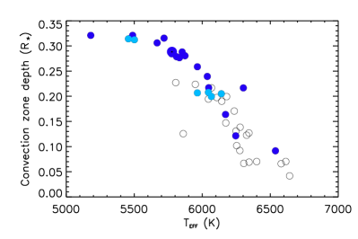
The limit in $T_{\rm eff}$ can probably be attributed to the Kraft break (e.g., Kraft 1967), where at around $6250$ K, these hotter stars rotate much faster as a result of a lack of a deep convective envelope, in which magnetic braking could slow the star down. The depth of the convective region is shown as a function of $T_{\rm eff}$ in Fig. 11, and stars with regions larger than approximately 0.2 stellar radii satisfy this criterion. This limit is also compatible with the proposed mass limit of approximately 1.3 M_⊙ where a transition in envelope convection takes place. The negative slope of the surface correction at $\nu_{\rm max}$ is also found to increase with increasing mass (becoming flatter), again indicating a change in convective zone properties and $T_{\rm eff}$. The limit in $\log g$ points toward a transition from the main-sequence to the subgiant phase where the convective envelope begins to deepen.

These limits are imposed by the physical structure of the star itself, but no quantitative measure of $a_{0}$ can be deduced from the observed and/or inferred stellar properties at this stage, except for a slight linear dependence of $a_{0}$ with $\langle\Delta\nu\rangle$, $\nu_{\rm max}$, or $\log g$ with a rather large scatter.

Figure 10: Distribution of observed (top panels) and derived parameters (lower panels) for the selected subsample of stars (open circles). The dark and light blue filled dots represent the stars with $Q\leq 1.0$ and 1.2. The regions are delimited by dashed lines within which we infer that the Kjeldsen et al. (2008) surface prescription should be useful.

Table 6: Stellar property regimes where the Kjeldsen et al. (2008) surface correction is useful.

Property	Value
$\log g$ (cgs)	$\geq$	4.2
$T_{\rm eff}$ (K)	$\leq$	6200
$\langle\Delta\nu\rangle$ ($\mu$Hz)	$\geq$	80
$\nu_{\rm max}$ ($\mu$Hz)	$\geq$	1700
$a_{0}$ ($\mu$Hz)	$\leq$	-6
$R$ (R⊙)	$\leq$	1.5
$M$ (M⊙)	$\leq$	1.3
$L$ (L⊙)	$\leq$	2.5

6 Summary

The high-quality and long-term photometric time series provided by Kepler has enabled an unprecedented precision on asteroseismic data of stars like the Sun. Thanks to the very high precision, we could use the frequency separation ratios along with spectroscopic temperatures and metallicities to infer stellar properties of the Sun and 57 Kepler stars, comprising solar analogs, active stars, components of binaries, and planetary hosts, with a precision of the same quality when using the individual frequencies. Median uncertainties on radius and mass are 1% and 3%, while uncertainties on the age compared to the estimated main-sequence lifetime are typically 7% or 11% compared to the absolute age. These realistic uncertainties account for unbiased determinations of mixing-length parameter and initial chemical composition. Along with the physical stellar properties, we also derived the interstellar absorption and distances to each star, and where the rotation period was available, we derived the rotational velocity. For nine stars our derivation of radii, luminosities, and distances are in very good agreement with independently measured values. Our inferred ages are validated for the Sun and by comparing the ages of the individual components of the binary system 16 Cyg A and B.

From an analysis of our derived properties for the full sample we investigated the dependence of the mixing-length parameter with stellar properties and found it to correlate with $\log g$ and $T_{\rm eff}$ , just as proposed by Magic et al. (2015) from 3D RHD simulations of convective envelopes. We also derived a linear expression relating the mean value of the $r_{02}$ frequency separation ratios directly to the age of the star, which yields an age of 4.7 Gyr for the Sun.

By selecting a subsample of the stars using a $\chi^{2}_{N}$ threshold, we investigated the usefulness of the Kjeldsen et al. (2008) empirical correction for the surface effects across a broad range of stellar parameters, and we found that it is useful, but only in certain regimes, as also suggested by the theoretical study of Schmitt & Basu (2015). This is of particular interest for stars with much shorter time series, where the precision on the individual frequencies or the number of radial orders is not high enough to constrain the stellar modeling. In particular, this will be the case for the forthcoming NASA TESS mission, where some stars with ecliptic latitude $|b|\lesssim 60^{\circ}$ will be observed continuously for only 27 days, along with the step-and-stare phase of the future PLATO mission (launch 2024).

7 Perspectives

In this work we used $T_{\rm eff}$ and [M/H] as the only complementary data to the asteroseismic data. However, within a year from now, we will have a homogenous set of microarcsecond precision parallaxes that will give access to the intrinsic luminosity of the star. This quantity is sensitive to the interior stellar composition. While today we have very high precision radii along with other properties, degeneracies in model parameters, such as the mass and initial helium abundance (e.g., Metcalfe et al. 2009; Lebreton & Goupil 2014) limit the full exploitation of asteroseismic data for testing stellar interior models and improving precision on model parameters. The forthcoming Gaia data in Release 2 promise to overcome this obstacle and thus provide even higher precision radii and ages, along with constraints on interior and initial chemical composition, and thus pushing stellar models to their limit.

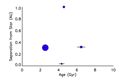
We highlight the importance of the precise characterisation of exoplanetary systems using asteroseismic data. In this work, we determined the radius and age of three planetary hosts (KIC 9414417, KIC 9955598, and KIC 10963065). Combining our data with those of Batalha et al. (2013) constrains the planetary and orbital parameters. We illustrate this in Fig. 12, where we depict the separation of the planet and host as a function of stellar age (including the Earth). The sizes of the symbols are indicative of the planetary radius, and the equilibrium temperature decreases with distance from the host. The diversity of planetary systems can be easily noted, and such an analysis of a larger sample of planetary candidates will yield important constraints on the formation and evolution of planetary systems. The future TESS and PLATO missions targeting bright stars with asteroseismic characterization promise to be a goldmine for not only exoplanetary physics, but with access to microarcsecond parallaxes and homogenous multiband photometry, also for stellar and Galactic physics.

Figure 11: Fractional depth of the convection zone as a function of $T_{\rm eff}$ for our selected subsample of stars. The color-coding is the same as Fig. 10.

Figure 12: Age of planet and separation from host. Symbol sizes represent planetary radius, and equilibrium temperature decreases with distance from the host. Age and radius are taken from this work, while other parameters are taken from (Batalha et al. 2013). The Earth is shown at 1 AU.

Appendix A Supplementary material

Figure 13: Echelle diagrams for two stars where the surface correction appears to be useful (top) and for two stars where the correction is not useful (lower). Crosses are observed frequencies, and black circles are corrected frequencies. The value of $\epsilon$ is an arbitrary shift in x-axis for display purposes.

Table 7: Derived stellar properties of Kepler targets with M $\sim$ 1.2 M_⊙ with or without diffusion of helium

KIC ID	$R$	$M$	Age	$L$	$\log g$	[M/H]
	(R⊙)	(M⊙)	(Gyr)	(L⊙)	(dex)	(dex)
no diffusion
9139151	1.132	1.11	1.96	1.80	4.375	-0.01
12009504	1.366	1.10	3.38	2.39	4.210	-0.01
6225718	1.227	1.15	2.29	2.09	4.320	-0.10
diffusion
1225814	1.595	1.26	5.04	2.81	4.129	0.05
5184732	1.356	1.25	4.68	1.82	4.269	0.25
8150065	1.397	1.21	3.12	2.54	4.228	-0.05
8179536	1.348	1.25	1.93	2.64	4.274	-0.05
7771282	1.631	1.26	3.34	3.65	4.116	-0.03
10454113	1.250	1.20	1.98	2.04	4.320	-0.04

References

- Ammons et al. (2006) Ammons, S. M., Robinson, S. E., Strader, J., et al. 2006, ApJ, 638, 1004
- Angulo et al. (1999) Angulo, C., Arnould, M., Rayet, M., et al. 1999, Nuclear Physics A, 656, 3
- Angulo et al. (2005) Angulo, C., Champagne, A. E., & Trautvetter, H.-P. 2005, Nuclear Physics A, 758, 391
- Appourchaux et al. (2015) Appourchaux, T., Antia, H. M., Ball, W., et al. 2015, A&A, 582, A25
- Appourchaux et al. (2012) Appourchaux, T., Chaplin, W. J., García, R. A., et al. 2012, A&A, 543, A54
- Arentoft et al. (2008) Arentoft, T., Kjeldsen, H., Bedding, T. R., et al. 2008, ApJ, 687, 1180
- Baglin et al. (2006) Baglin, A., Auvergne, M., Barge, P., et al. 2006, in ESA Special Publication, Vol. 1306, The CoRoT Mission Pre-Launch Status - Stellar Seismology and Planet Finding, ed. M. Fridlund, A. Baglin, J. Lochard, & L. Conroy, 33
- Ball & Gizon (2014) Ball, W. H. & Gizon, L. 2014, A&A, 568, A123
- Batalha et al. (2013) Batalha, N. M., Rowe, J. F., Bryson, S. T., et al. 2013, ApJS, 204, 24
- Bazot (2013) Bazot, M. 2013, in EAS Publications Series, Vol. 63, EAS Publications Series, ed. G. Alecian, Y. Lebreton, O. Richard, & G. Vauclair, 105–114
- Bedding et al. (2001) Bedding, T. R., Butler, R. P., Kjeldsen, H., et al. 2001, ApJ, 549, L105
- Benomar et al. (2014a) Benomar, O., Belkacem, K., Bedding, T. R., et al. 2014a, ApJ, 781, L29
- Benomar et al. (2014b) Benomar, O., Masuda, K., Shibahashi, H., & Suto, Y. 2014b, PASJ, 66, 94
- Böhm-Vitense (1958) Böhm-Vitense, E. 1958, ZAp, 46, 108
- Bonaca et al. (2012) Bonaca, A., Tanner, J. D., Basu, S., et al. 2012, ApJ, 755, L12
- Borucki et al. (2010) Borucki, W. J., Koch, D., Basri, G., et al. 2010, Science, 327, 977
- Bouchy & Carrier (2002) Bouchy, F. & Carrier, F. 2002, A&A, 390, 205
- Brown et al. (1991) Brown, T. M., Gilliland, R. L., Noyes, R. W., & Ramsey, L. W. 1991, ApJ, 368, 599
- Buchhave et al. (2014) Buchhave, L. A., Bizzarro, M., Latham, D. W., et al. 2014, Nature, 509, 593
- Buchhave & Latham (2015) Buchhave, L. A. & Latham, D. W. 2015, ApJ, 808, 187
- Buchhave et al. (2012) Buchhave, L. A., Latham, D. W., Johansen, A., et al. 2012, Nature, 486, 375
- Carrier & Bourban (2003) Carrier, F. & Bourban, G. 2003, A&A, 406, L23
- Carrier et al. (2007) Carrier, F., Kjeldsen, H., Bedding, T. R., et al. 2007, A&A, 470, 1059
- Casagrande et al. (2014) Casagrande, L., Silva Aguirre, V., Stello, D., et al. 2014, ApJ, 787, 110
- Ceillier et al. (2016) Ceillier, T., van Saders, J., García, R. A., et al. 2016, MNRAS, 456, 119
- Chaplin et al. (2010) Chaplin, W. J., Appourchaux, T., Elsworth, Y., et al. 2010, ApJ, 713, L169
- Chaplin et al. (2014) Chaplin, W. J., Basu, S., Huber, D., et al. 2014, ApJS, 210, 1
- Chaplin & Miglio (2013) Chaplin, W. J. & Miglio, A. 2013, ARA&A, 51, 353
- Christensen-Dalsgaard (2008a) Christensen-Dalsgaard, J. 2008a, Ap&SS, 316, 113
- Christensen-Dalsgaard (2008b) Christensen-Dalsgaard, J. 2008b, Ap&SS, 316, 13
- Christensen-Dalsgaard et al. (1995) Christensen-Dalsgaard, J., Bedding, T. R., & Kjeldsen, H. 1995, ApJ, 443, L29
- Creevey et al. (2012) Creevey, O. L., Thévenin, F., Boyajian, T. S., et al. 2012, A&A, 545, A17
- Davies et al. (2016) Davies, G. R., Aguirre, V. S., Bedding, T. R., et al. 2016, MNRAS, 456, 2183
- Davies et al. (2015) Davies, G. R., Chaplin, W. J., Farr, W. M., et al. 2015, MNRAS, 446, 2959
- Di Mauro et al. (2003) Di Mauro, M. P., Christensen-Dalsgaard, J., Kjeldsen, H., Bedding, T. R., & Paternò, L. 2003, A&A, 404, 341
- Eggenberger et al. (2004) Eggenberger, P., Charbonnel, C., Talon, S., et al. 2004, A&A, 417, 235
- Ferguson et al. (2005) Ferguson, J. W., Alexander, D. R., Allard, F., et al. 2005, ApJ, 623, 585
- Fernandes & Monteiro (2003) Fernandes, J. & Monteiro, M. J. P. F. G. 2003, A&A, 399, 243
- Flower (1996) Flower, P. J. 1996, ApJ, 469, 355
- Fröhlich et al. (1995) Fröhlich, C., Romero, J., Roth, H., et al. 1995, Sol. Phys., 162, 101
- García et al. (2014) García, R. A., Ceillier, T., Salabert, D., et al. 2014, A&A, 572, A34
- Gilliland et al. (2010) Gilliland, R. L., Jenkins, J. M., Borucki, W. J., et al. 2010, ApJ, 713, L160
- Gough (1990) Gough, D. O. 1990, in Lecture Notes in Physics, Berlin Springer Verlag, Vol. 367, Progress of Seismology of the Sun and Stars, ed. Y. Osaki & H. Shibahashi, 283
- Grevesse & Noels (1993) Grevesse, N. & Noels, A. 1993, in Origin and Evolution of the Elements, ed. N. Prantzos, E. Vangioni-Flam, & M. Casse, 15–25
- Grevesse & Sauval (1998) Grevesse, N. & Sauval, A. J. 1998, Space Sci. Rev., 85, 161
- Gruberbauer et al. (2012) Gruberbauer, M., Guenther, D. B., & Kallinger, T. 2012, ApJ, 749, 109
- Guenther & Brown (2004) Guenther, D. B. & Brown, K. I. T. 2004, ApJ, 600, 419
- Houdek & Gough (2011) Houdek, G. & Gough, D. O. 2011, MNRAS, 418, 1217
- Houdek et al. (2016) Houdek, G., Trampedach, R., Aarslev, M. J., & Christensen-Dalsgaard, J. 2016, ArXiv e-prints
- Huber et al. (2013) Huber, D., Chaplin, W. J., Christensen-Dalsgaard, J., et al. 2013, ApJ, 767, 127
- Huber et al. (2012) Huber, D., Ireland, M. J., Bedding, T. R., et al. 2012, ApJ, 760, 32
- Huber et al. (2014) Huber, D., Silva Aguirre, V., Matthews, J. M., et al. 2014, ApJS, 211, 2
- Iglesias & Rogers (1996) Iglesias, C. A. & Rogers, F. J. 1996, ApJ, 464, 943
- Kallinger et al. (2010) Kallinger, T., Gruberbauer, M., Guenther, D. B., Fossati, L., & Weiss, W. W. 2010, A&A, 510, A106
- Kjeldsen et al. (2008) Kjeldsen, H., Bedding, T. R., & Christensen-Dalsgaard, J. 2008, ApJ, 683, L175
- Kjeldsen et al. (1995) Kjeldsen, H., Bedding, T. R., Viskum, M., & Frandsen, S. 1995, AJ, 109, 1313
- Kraft (1967) Kraft, R. P. 1967, ApJ, 150, 551
- Lebreton & Goupil (2014) Lebreton, Y. & Goupil, M. J. 2014, A&A, 569, A21
- Lebreton & Montalbán (2009) Lebreton, Y. & Montalbán, J. 2009, in IAU Symposium, Vol. 258, The Ages of Stars, ed. E. E. Mamajek, D. R. Soderblom, & R. F. G. Wyse, 419–430
- Lund et al. (2014) Lund, M. N., Lundkvist, M., Silva Aguirre, V., et al. 2014, A&A, 570, A54
- Lund et al. (2017) Lund, M. N., Silva Aguirre, V., Davies, G. R., et al. 2017, ApJ, 835, 172
- Magic et al. (2015) Magic, Z., Weiss, A., & Asplund, M. 2015, A&A, 573, A89
- Marigo et al. (2008) Marigo, P., Girardi, L., Bressan, A., et al. 2008, A&A, 482, 883
- Masana et al. (2006) Masana, E., Jordi, C., & Ribas, I. 2006, A&A, 450, 735
- Mathur et al. (2012) Mathur, S., Metcalfe, T. S., Woitaszek, M., et al. 2012, ApJ, 749, 152
- Metcalfe et al. (2012) Metcalfe, T. S., Chaplin, W. J., Appourchaux, T., et al. 2012, ApJ, 748, L10
- Metcalfe & Charbonneau (2003) Metcalfe, T. S. & Charbonneau, P. 2003, Journal of Computational Physics, 185, 176
- Metcalfe et al. (2009) Metcalfe, T. S., Creevey, O. L., & Christensen-Dalsgaard, J. 2009, ApJ, 699, 373
- Metcalfe et al. (2015) Metcalfe, T. S., Creevey, O. L., & Davies, G. R. 2015, ApJ, 811, L37
- Metcalfe et al. (2014) Metcalfe, T. S., Creevey, O. L., Doğan, G., et al. 2014, ApJS, 214, 27
- Metcalfe et al. (2010) Metcalfe, T. S., Monteiro, M. J. P. F. G., Thompson, M. J., et al. 2010, ApJ, 723, 1583
- Michaud & Proffitt (1993) Michaud, G. & Proffitt, C. R. 1993, in Astronomical Society of the Pacific Conference Series, Vol. 40, IAU Colloq. 137: Inside the Stars, ed. W. W. Weiss & A. Baglin, 246–259
- Michel et al. (2008) Michel, E., Baglin, A., Auvergne, M., et al. 2008, Science, 322, 558
- Pinsonneault et al. (2012) Pinsonneault, M. H., An, D., Molenda-Żakowicz, J., et al. 2012, ApJS, 199, 30
- Pinsonneault et al. (2014) Pinsonneault, M. H., Elsworth, Y., Epstein, C., et al. 2014, ApJS, 215, 19
- Ramírez et al. (2009) Ramírez, I., Meléndez, J., & Asplund, M. 2009, A&A, 508, L17
- Rauer et al. (2014) Rauer, H., Catala, C., Aerts, C., et al. 2014, Experimental Astronomy, 38, 249
- Ricker et al. (2015) Ricker, G. R., Winn, J. N., Vanderspek, R., et al. 2015, Journal of Astronomical Telescopes, Instruments, and Systems, 1, 014003
- Rogers & Nayfonov (2002) Rogers, F. J. & Nayfonov, A. 2002, ApJ, 576, 1064
- Rosenthal (1997) Rosenthal, C. S. 1997, in Astrophysics and Space Science Library, Vol. 225, SCORe’96 : Solar Convection and Oscillations and their Relationship, ed. F. P. Pijpers, J. Christensen-Dalsgaard, & C. S. Rosenthal, 145–160
- Roxburgh & Vorontsov (2003) Roxburgh, I. W. & Vorontsov, S. V. 2003, A&A, 411, 215
- Schmitt & Basu (2015) Schmitt, J. R. & Basu, S. 2015, ApJ, 808, 123
- Schultheis et al. (2014) Schultheis, M., Zasowski, G., Allende Prieto, C., et al. 2014, AJ, 148, 24
- Silva Aguirre et al. (2013) Silva Aguirre, V., Basu, S., Brandão, I. M., et al. 2013, ApJ, 769, 141
- Silva Aguirre et al. (2015) Silva Aguirre, V., Davies, G. R., Basu, S., et al. 2015, MNRAS, 452, 2127
- Silva Aguirre et al. (2017) Silva Aguirre, V., Lund, M. N., Antia, H. M., et al. 2017, ApJ, 835, 173
- Skrutskie et al. (2006) Skrutskie, M. F., Cutri, R. M., Stiening, R., et al. 2006, AJ, 131, 1163
- Thévenin et al. (2002) Thévenin, F., Provost, J., Morel, P., et al. 2002, A&A, 392, L9
- Thoul et al. (2003) Thoul, A., Scuflaire, R., Noels, A., et al. 2003, A&A, 402, 293
- Torres (2010) Torres, G. 2010, AJ, 140, 1158
- Trampedach et al. (2017) Trampedach, R., Aarslev, M. J., Houdek, G., et al. 2017, MNRAS, 466, L43
- Trampedach et al. (2014) Trampedach, R., Stein, R. F., Christensen-Dalsgaard, J., Nordlund, Å., & Asplund, M. 2014, MNRAS, 442, 805
- van Leeuwen (2007) van Leeuwen, F. 2007, A&A, 474, 653
- White et al. (2013) White, T. R., Huber, D., Maestro, V., et al. 2013, MNRAS, 433, 1262
- Yıldız et al. (2006) Yıldız, M., Yakut, K., Bakış, H., & Noels, A. 2006, MNRAS, 368, 1941